Analytical contradictions
of the ’fixed - node’ density matrix

Abstract

Over the last decades the ’fixed-node method’ has been used for a numerical treatment of thermodynamic properties of strongly correlated Fermi systems. In this work correctness of the ’fixed -node method’ for ideal Fermi systems has been analytically analyzed. It is shown that the ’fixed-node’ prescription of calculation of the density matrix leads to contradictions even for two ideal fermions. The main conclusion of this work is that the ’fixed-node method’ can not reproduce the fermion density matrices and should be considered as uncontrolled empirical approach in treatment of thermodynamics of Fermi systems.

I Introduction

Over the last decades significant progress has been observed in theoretical studies of thermodynamic properties of strongly correlated fermions at non-zero temperatures, which is mainly conditioned by the application of numerical simulations (see review Ceprl1 ). The reason for this success is the possibility of an explicit representation of the density matrix in the form of the Wiener path integrals Feynm and application of the Monte Carlo method for further calculations. The main difficulty for path integral Monte Carlo (PIMC) studies of Fermi systems results from the requirement of antisymmetrization of the density matrix Feynm . Then all thermodynamic quantities are presented as the sum of alternating sign terms related to even and odd permutations and are equal to the small difference of two large numbers, which are the sums of positive and negative terms. The numerical calculation in this case is severely hampered. This difficulty is known in the literature as the ’sign problem’. To overcome this issue some approaches have been developed, among which the ’fixed-node method’ Ceprl1 ; Ceprl2 ; Ceprl3 ; Militz is widely known.

To avoid sign problem at calculation of the path integral representation of the fermion density matrix the authors of Ceprl2 ; Ceprl3 suggested ’the path integral solution of the Bloch equation without minus signs’. This means that they introduced restriction of integration over paths by the domain, where additional ’trial antisymmetric density matrix’ is not negative. The author of Ceprl2 ; Ceprl3 claimed that this restriction of path integration gives the exact solution of the Bloch equation in the form of path integrals with standard antisymmetric initial condition.

The purpose of this work is to give an analytical proof that this restriction results in contradictions at explicit calculations of the density matrix even for two ideal fermions. The analogous contradictions have been analytically obtained twelve years ago in cluster from virial decomposition of the many fermion ’fixed-node’ density matrix’. However paper cluster is very difficult for understanding as used the Rueele algebraic approach Ruelle and was missed by the scientific community. This is the reason to discuss correctness of the ’fixed - node method’ once more using more simple mathematical technique. The main result of this work and paper cluster is that the ’fixed–node method’ can not reproduce even the well known ideal fermion density matrix and should be considered as an uncontrolled empirical approach in treatment of thermodynamics of fermions.

II Density matrix by the ’fixed - node method’

Thermodynamic values of the fermion quantum system at non-zero temperature are defined by the appropriate derivatives of the logarithm of the partition function $Q_{N}=Tr\{\rho\}$. Here $\rho=\exp(-\beta\hat{H})$ is the density matrix of a quantum system of particles with the Hamiltonian $\hat{H}=\hat{K}+\hat{U}$ equal to the sum of kinetic $\hat{K}$ and potential energy $\hat{U}$ operators, while $\beta=1/k_{B}T$ . For our purposes it is enough to consider one dimensional (1D) system of two ideal fermions. So $\hat{U}\equiv 0$, while the kinetic energy operator is the sum of two kinetic energy operators related to each particle $\hat{K}=\hat{K_{1}}+\hat{K_{2}}$. Density matrix is the solution of the operator Bloch equation

$$\frac{\partial\hat{\rho}}{\partial\beta}=-\hat{K}\hat{\rho}$$ (1)

with the initial condition $\hat{\rho}|_{\beta=0}=\hat{1}$.

This operator equation in coordinate representation for fermions can be written in the form Ceprl2 ; Ceprl3

$$\frac{\partial\rho_{F}(R,R_{0};\beta)}{\partial\beta}=-\hat{K}(R)\rho_{F}(R,R_{0};\beta)$$ (2)

with the initial condition

$$\rho_{F}(R,R_{0};0)=\frac{1}{N!}\sum_{P}(-1)^{\kappa P}\delta(R-PR_{0})$$ (3)

where $R$ is the set of coordinates of all particles. One of the possible coordinate representation of the fermion density matrix looks like

$$\rho_{F}(R,R_{0};\beta)=\frac{1}{N!}\sum_{\alpha}\exp(-\beta E_{\alpha})\phi^{*}_{\alpha}(R)\phi_{\alpha}(R_{0})$$ (4)

where the sum is over the complete set of antisymmetric eigenfunctions $\phi_{\alpha}(R)$ of $\hat{H}$.

Another exact popular coordinate representation of operator $\hat{\rho}$ follows from the operator identity $e^{-\beta\hat{K}}\equiv e^{-\Delta\beta{\hat{K}}}\cdots e^{-\Delta\beta{\hat{K}}}\dots e^{-\Delta\beta{\hat{K}}}$for any (even of oder unity) integer fixed $M$. Here the r.h.s. contains $M$ identical factors with $\Delta\beta=\beta/M$. So one can exactly present the ideal density matrix in the form of finite– difference expression of the path integral

$$\rho_{F}(R_{M},R_{0};\beta)=\frac{1}{N!}\sum_{P}(-1)^{\kappa_{P}}\int dR_{1}\cdots dR_{M-1}\left(\prod_{k=1}^{M-1}\rho(R_{k-1},R_{k};\Delta\beta)\right)\rho(R_{M-1},PR_{M};\Delta\beta)$$ (5)

where $N$ is the number of fermions. For $N=2$ arguments are two dimensional (2D) vectors composed by the coordinates of the first and second particle on $1D$ axes $X^{(1)}$ and $X^{(2)}$ and $\rho(R_{k-1},R_{k};\Delta\beta)$ are distinguishable particle density matrices. Antisymmetry is put in by the antisymmetrization. The sum runs over all permutations with parity $\kappa_{P}$ acting on indexes of particles. The density matrix is function of the space 2D arguments $R_{M},R_{0}$ on ($X^{(1)},X^{(2)}$) plane and inverse temperature (image time) $\beta$. Below we are going to discuss the boundary conditions of the certain domain on the ($X^{(1)},X^{(2)}$) plane and mentioned before the initial conditions on $\beta$ of the parabolic equation (2).

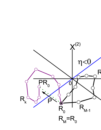
Figure 1: (Color online) Configurational space of two free fermions. Plotted are the paths related to the two possible permutations: identical (below line $\gamma$) and non-identical (crossing line $\gamma$) permutations.

Mathematical meaning of expression (5) for density matrix of two particles is illustrated by Fig. 1, where vectors $R_{k}$ are presented by circles (called often as ’beads’), while density matrices $\rho(R_{k-1},R_{k};\Delta\beta)$ are denoted by segments of lines. Sometimes instead of coordinate $\left\{X^{(1)}_{k},X^{(2)}_{k}\right\}$ it is convenient to use coordinates $\left\{\gamma_{k},\eta_{k}\right\}$ defined by expressions $\gamma_{k}=0.5\left(X^{(1)}_{k}+X^{(2)}_{k}\right)$ and $\eta_{k}=\left(X^{(1)}_{k}-X^{(2)}_{k}\right)$, so $R_{k}=\left\{X^{(1)}_{k},X^{(2)}_{k}\right\}=\left\{\gamma_{k},\eta_{k}\right\}$. Modulus of Jacobian related to the change of variables of integration in Eq. (5) from the system of coordinates $\left\{X^{(1)}_{k},X^{(2)}_{k}\right\}$ to the system $\left\{\gamma_{k},\eta_{k}\right\}$ is equal to unity. Action of perturbation $P$ is illustrated in Fig. 1 by the arrow with letter $P$ (see Fig. 1). For two fermions the sum over permutations is reduced to the sum of contributions of identical and non identical permutations with opposite signs. The density matrix has the following general properties:

$$\rho_{F}(R,R_{0};\beta)=\rho_{F}(R_{0},R;\beta)=(-1)^{\kappa P}\rho_{F}(PR,R_{0};\beta)$$ (6)

For further comparisons with the ’fixed - node’ density matrix let us remind the solution of the Bloch equation (2) with the initial condition (3). Density matrices in (5) are well known for ideal particles and can be written in the form Feynm :

$$\rho(R_{k-1},R_{k};\Delta\beta)=\frac{\exp\left(-\frac{\pi|R_{k}-R_{k-1}|^{2}}{\tilde{\lambda}^{2}}\right)}{\tilde{\lambda}^{2}}=\frac{\exp\left(-\frac{2\pi|\gamma_{k}-\gamma_{k-1}|^{2}}{\tilde{\lambda}^{2}}\right)\exp\left(-\frac{\pi|\eta_{k}-\eta_{k-1}|^{2}}{2\tilde{\lambda}^{2}}\right)}{\tilde{\lambda}^{2}}$$ (7)

where $\tilde{\lambda}^{2}=2\pi\hbar^{2}\Delta\beta/m$ is the thermal wave length related to $\Delta\beta$. The last factor in (5) for permutation $P$ has the form

$$\rho(R_{M-1},PR_{M};\Delta\beta)=\frac{\exp\left(-\frac{\pi|PR_{M}-R_{M-1}|^{2}}{\tilde{\lambda}^{2}}\right)}{\tilde{\lambda}^{2}}=\frac{\exp\left(-\frac{2\pi|P\gamma_{M}-\gamma_{M-1}|^{2}}{\tilde{\lambda}^{2}}\right)\exp\left(-\frac{\pi|P\eta_{M}-\eta_{M-1}|^{2}}{2\tilde{\lambda}^{2}}\right)}{\tilde{\lambda}^{2}}.$$ (8)

So the exact well known expression for two particle antisymmetrized density matrix looks like Feynm

$$\rho_{F}(R_{M},R_{0};\beta)=\frac{1}{2}\int dR_{1}\cdots dR_{M-1}\left(\prod_{k=1}^{M-1}\frac{\exp\left(-\frac{\pi|R_{k}-R_{k-1}|^{2}}{\tilde{\lambda}^{2}}\right)}{\tilde{\lambda}^{2}}\right)\frac{\exp\left(-\frac{2\pi|\gamma_{M}-\gamma_{M-1}|^{2}}{\tilde{\lambda}^{2}}\right)}{\tilde{\lambda}}$$ (9)

$$\times\left\{\frac{\exp\left(-\frac{\pi|\eta_{M}-\eta_{M-1}|^{2}}{2\tilde{\lambda}^{2}}\right)-\exp\left(-\frac{\pi|P\eta_{M}-\eta_{M-1}|^{2}}{2\tilde{\lambda}^{2}}\right)}{\tilde{\lambda}}\right\}$$

$$\equiv \frac{1}{2}\frac{\exp\left(-\frac{2\pi|\gamma_{M}-\gamma_{0}|^{2}}{\lambda^{2}}\right)}{\lambda}\left\{\frac{\exp\left(-\frac{\pi|\eta_{M}-\eta_{0}|^{2}}{2\lambda^{2}}\right)-\exp\left(-\frac{\pi|P\eta_{M}-\eta_{0}|^{2}}{2\lambda^{2}}\right)}{\lambda}\right\}$$

with $\lambda^{2}=2\pi\hbar^{2}\beta/m$, $P\gamma_{M}=\gamma_{M}$ and $P\eta_{M}=-\eta_{M}$. If $\left\{\gamma_{M},\eta_{M}\right\}=\left\{\gamma_{0},\eta_{0}\right\}$ then $P\gamma_{M}=\gamma_{0}$ and $P\eta_{M}=-\eta_{0}$ (see Fig. 1).

To avoid ’sign problem’ at calculation of the path integral representation of the fermion density matrix the authors of Ceprl2 ; Ceprl3 suggested the ’fixed - node’ ’the path integral solution of the Bloch equation without minus signs’. The authors of Ceprl2 ; Ceprl3 denotes the second argument $R_{0}$ of the density matrix as the ’reference point’ and ’the set of points $R_{t}$ for which there exists a continuous ’space–imaginary time’ path with $\rho_{F}(R,R_{0};t^{\prime})>0$ for $0\leq t^{\prime}\leq\beta$ the reach of $R_{0}$ or $\Gamma(R_{0},\beta)$’. For two ideal fermions the reach can be analytically obtained Ceprl2 ; Ceprl3 . The reach (the half plane $\eta>0$) for $\eta_{0}>0$ is shown in Fig. 1. The reach does not depend on temperature.

According to the papers Ceprl2 ; Ceprl3 ’It is a simple matter (see Appendix C) to show that the problematic INITIAL CONDITION, Eq. (3), can be replaced by a zero boundary conditions on the SURFACE of the reach. It follows because the fermion density matrix is a unique solution to the Bloch equation (2) with the zero BOUNDARY CONDITION.’ However the Bloch equation (2) with the zero boundary conditions is linear equation and, besides the trivial solution identically equal to zero, has an infinite number of solutions distinguishing at least by constant factors, while the Bloch equation (2) with initial condition (3) has really a unique solution.

Let us consider ’fixed – node’ approach to calculation of the density matrices in the $\gamma-\eta$ plane (see Fig. 1). The author of Ceprl2 ; Ceprl3 claimed that to obtain the ’fixed – node’ density matrix ’one simply restricts the paths in Eq. (5) to lie in the $\Gamma(R_{0},\beta)$’. This means that restriction of integration over $R_{1},\cdots,R_{M-1}$ in (5) by the reach has to give the exact solution of Eq. (2) with initial condition (3). The fallaciousness of this statement for $M=2$ as well as for arbitrary integer $M$ can be easily proved by explicit integration over variables $R_{1},\cdots,R_{M-1}$ in the reach for 1D two ideal fermions. The boundary surface of the 2D reach for two ideal fermions is exactly known and according to papers Ceprl2 ; Ceprl3 is the line $\eta=0$ in Fig. 1. So according to the ’fixed-node’ prescription the density matrix in the whole configurational space (in both half planes ($\eta>0$ and $\eta<0$) ($\eta_{M},\eta_{0}\in\{X^{(1)},X^{(2)}\}$)) looks like

$$\rho_{F}(R_{M},R_{0};\beta)=\frac{C_{1}}{2}\int dR_{1}\cdots dR_{M-1}\left(\prod_{k=1}^{M-1}\frac{\exp\left(-\frac{\pi|R_{k}-R_{k-1}|^{2}}{\tilde{\lambda}^{2}}\right)}{\tilde{\lambda}^{2}}\right)\frac{\exp\left(-\frac{2\pi|\gamma_{M}-\gamma_{M-1}|^{2}}{\tilde{\lambda}^{2}}\right)}{\tilde{\lambda}}$$

$$\times\left\{\frac{\exp\left(-\frac{\pi|\eta_{M}-\eta_{M-1}|^{2}}{2\tilde{\lambda}^{2}}\right)-\exp\left(-\frac{\pi|P\eta_{M}-\eta_{M-1}|^{2}}{2\tilde{\lambda}^{2}}\right)}{\tilde{\lambda}}\right\}\theta(\eta_{0})\theta(\eta_{1})\cdots\theta(\eta_{M})$$

$$+\frac{C_{2}}{2}\int dR_{1}\cdots dR_{M-1}\left(\prod_{k=1}^{M-1}\frac{\exp\left(-\frac{\pi|R_{k}-R_{k-1}|^{2}}{\tilde{\lambda}^{2}}\right)}{\tilde{\lambda}^{2}}\right)\frac{\exp\left(-\frac{2\pi|\gamma_{M}-\gamma_{M-1}|^{2}}{\tilde{\lambda}^{2}}\right)}{\tilde{\lambda}}$$

$$\times\left\{\frac{\exp\left(-\frac{\pi|\eta_{M}-\eta_{M-1}|^{2}}{2\tilde{\lambda}^{2}}\right)-\exp\left(-\frac{\pi|P\eta_{M}-\eta_{M-1}|^{2}}{2\tilde{\lambda}^{2}}\right)}{\tilde{\lambda}}\right\}\theta(-\eta_{0})\theta(-\eta_{1})\cdots\theta(-\eta_{M}),$$ (10)

where $\theta(\eta)$ is the theta function equal to zero for $\eta<0$ and equal to unity in the opposite case $\eta\geq 0$ . The theta functions restrict to the reach the domains of integration. Now assume that all ’basic statements’ of papers Ceprl2 ; Ceprl3 are correct, then using the mentioned above general properties of the density matrix we have to admit that integration over $R_{2}\cdots,R_{M-1}$ in the reach gives the exact solution of Eq. (2) with initial condition (3). So the density matrix in the ’fixed–node method’ (II) can be transformed to the following integral over the last variable $R_{1}$:

$$\rho_{F}(R_{M},R_{0};\beta)=\frac{1}{2}\int dR_{1}\frac{\exp\left(-\frac{\pi|R_{1}-R_{0}|^{2}}{\tilde{\lambda}^{2}}\right)}{\tilde{\lambda}^{2}}\frac{\exp\left(-\frac{2\pi|\gamma_{M}-\gamma_{1}|^{2}}{(M-1)\tilde{\lambda}^{2}}\right)}{\sqrt{(M-1)}\tilde{\lambda}}$$ (11)

$$\times[C_{1}\frac{\exp\left(-\frac{\pi|\eta_{M}-\eta_{1}|^{2}}{2(M-1)\tilde{\lambda}^{2}}\right)-\exp\left(-\frac{\pi|P\eta_{M}-\eta_{1}|^{2}}{2(M-1)\tilde{\lambda}^{2}}\right)}{\sqrt{(M-1)}\tilde{\lambda}}\theta(\eta_{0})\theta(\eta_{1})\theta(\eta_{M})$$

$$+C_{2}\frac{\exp\left(-\frac{\pi|\eta_{M}-\eta_{1}|^{2}}{2(M-1)\tilde{\lambda}^{2}}\right)-\exp\left(-\frac{\pi|P\eta_{M}-\eta_{1}|^{2}}{2(M-1)\tilde{\lambda}^{2}}\right)}{\sqrt{(M-1)}\tilde{\lambda}}\theta(-\eta_{0})\theta(-\eta_{1})\theta(-\eta_{M})]$$

$$=\frac{1}{2}\frac{\exp\left(-\frac{2\pi|\gamma_{M}-\gamma_{0}|^{2}}{\lambda^{2}}\right)}{2\lambda}[C_{1}\theta(\eta_{0})\theta(\eta_{M})$$

$$\times\frac{\exp\left(-\frac{\pi|\eta_{M}-\eta_{0}|^{2}}{2\lambda^{2}}\right)\xi((M-1)\eta_{0}+\eta_{M})-\exp\left(-\frac{\pi|P\eta_{M}-\eta_{0}|^{2}}{2\lambda^{2}}\right)\xi((M-1)\eta_{0}+P\eta_{M})}{\lambda}$$

$$+C_{2}\theta(-\eta_{0})\theta(-\eta_{M})$$

$$\times\frac{\exp\left(-\frac{\pi|\eta_{M}-\eta_{0}|^{2}}{2\lambda^{2}}\right)\xi(-(M-1)\eta_{0}+\eta_{M})-\exp\left(-\frac{\pi|P\eta_{M}-\eta_{0}|^{2}}{2\lambda^{2}}\right)\xi(-(M-1)\eta_{0}+P\eta_{M})}{\lambda}]$$

where $\xi\left(z\right)=erfc\left(-\frac{\sqrt{\pi}z}{\sqrt{2M(M-1)}\tilde{\lambda}}\right)$

Thus instead of the unique density matrix (9) we have infinite number of the ’fixed – node’ density matrices (11) (due to the two arbitrary constants $C_{1}$ and $C_{2}$) taking the ’zero boundary conditions’ on the surface of the reach ($\eta_{M}=0$) for any finite $M\geq 2$. More over this density matrix depend on complementary error functions.

For further detail analysis of the function (11) let us consider the limit of $\Delta\beta\rightarrow 0$. Using definition of complementary error functions one can transform (11) to the form:

$$\rho_{F}(R_{M},R_{0};\beta)=\frac{\exp\left(-\frac{2\pi|\gamma_{M}-\gamma_{0}|^{2}}{\lambda^{2}}\right)}{4\lambda}$$

$$\times[C_{1}\theta(\eta_{0})\theta(\eta_{M})\frac{(\exp\left(-\frac{\pi|\eta_{M}-\eta_{0}|^{2}}{2\lambda^{2}}\right)-\exp\left(-\frac{\pi|P\eta_{M}-\eta_{0}|^{2}}{2\lambda^{2}}\right))(1+sign(\eta_{0}))}{\lambda}$$

$$+C_{2}\theta(-\eta_{0})\theta(-\eta_{M})\frac{(\exp\left(-\frac{\pi|\eta_{M}-\eta_{0}|^{2}}{2\lambda^{2}}\right)-\exp\left(-\frac{\pi|P\eta_{M}-\eta_{0}|^{2}}{2\lambda^{2}}\right))(1-sign(\eta_{0}))}{\lambda}]$$

$$=\frac{\exp\left(-\frac{2\pi|\gamma_{M}-\gamma_{0}|^{2}}{\lambda^{2}}\right)}{4\lambda}\frac{(\exp\left(-\frac{\pi|\eta_{M}-\eta_{0}|^{2}}{2\lambda^{2}}\right)-\exp\left(-\frac{\pi|P\eta_{M}-\eta_{0}|^{2}}{2\lambda^{2}}\right))}{\lambda}$$

$$\times[(C_{1}\theta(\eta_{0})\theta(\eta_{M})+C_{2}\theta(-\eta_{0})\theta(-\eta_{M}))$$

$$+(C_{1}\theta(\eta_{0})\theta(\eta_{M})-C_{2}\theta(-\eta_{0})\theta(-\eta_{M}))sign(\eta_{0})]$$ (12)

where

$$lim_{\Delta\beta\rightarrow 0}erfc\left(-\sqrt{\pi}\frac{\pm(M-1)\eta_{0}+P\eta_{M}}{\sqrt{2M(M-1)}\tilde{\lambda}}\right)$$

$$=1-lim_{\Delta\beta\rightarrow 0}erf\left(-\sqrt{\pi}\frac{\pm(M-1)\eta_{0}+P\eta_{M}}{\sqrt{2M(M-1)}\tilde{\lambda}}\right)=1\pm sign(\eta_{0})$$ (13)

and $erf$ is the error function. Here $sign(\eta_{0})$ is equal to plus unity for $\eta_{0}>0$ and minus unity for $\eta_{0}<0$. In the limit $\Delta\beta\rightarrow 0$ the ’fixed–node’ density matrix (II) for two arbitrary constants ($C_{1}$ and $C_{2}$) takes the ’zero boundary conditions’ on the surface of the reach ($\eta_{M}=0$).

To obtain the unique density matrix we need to specify constants $C_{1}$ and $C_{2}$. The ’fix-node’ density matrix (II) differs significantly from exact expressions Eq. (9). For $C_{1}=1$ and $C_{2}=0$ we have density matrix, which coincide with exact density matrix if both $\eta_{M}$ and $\eta_{0}$ are positive but if $\eta_{M}$ and $\eta_{0}$ have opposite sign the ’fixed-node’ density matrix is identically equal to zero and differs from exact density matrix. Generally the ’fix-node’ density matrix (II) is identically equal to zero if $\eta_{0}$ and $\eta_{M}$ are lying in opposite half planes ($\eta>0$ and $\eta<0$) of the $\gamma-\eta$ plane, while this is not the case for exact density matrix (9). The ’fix-node’ density matrix (II) contrary to the exact one is a non analytical function. Let us remind that all these expressions have been obtained at assumption that all ’basic statements’ of papers Ceprl2 ; Ceprl3 are correct. All these contradictions mean that the integration in the reach can not reproduce the exact solution of Eq. (2) with initial condition (3) in spite of the ’basic statement’ of papers Ceprl2 ; Ceprl3 .

An alternative approach for studies Fermi systems without replacement of initial conditions by zero boundary conditions for the Bloch equation is known in literature as the direct path integral Monte Carlo simulation (DPIMC) cluster ; Egger ; Imada ; FBF ; FFBK . In this approach the sum over all permutations is represented identically as a determinant, which can be exactly calculated by the direct methods of linear algebra. The accuracy of this approach depends only on the errors of the finite-dimensional approximations of the path integrals and can be improved systematically. Comparison with results of the DPIMC simulation show that the fixed – node method describes the thermodynamic properties of the strongly coupling fermions rather well at weak degeneracy, when the main contribution to the partition function comes from the identical permutation cluster ; FBF ; FFBK . The difference in obtained results increases systematically with the growth of the degeneracy at high density and low temperatures cluster ; FBF ; FFBK . The reason of this difference is in restriction by the ’reach’ of integration over ’beads’ in the ’fixed - node’ path integrals, which leads to wrong expression for density matrix even for two ideal fermions. This restriction results in uncontrolled errors in calculations of thermodynamic quantities due to the wrong description of statistical effects in the system of degenerate interacting and non interacting fermions .

III Conclusion

Let us sum up analytical contradictions following from the basic ’fixed – node’ prescription of calculation of the fermion density matrix (’one simply restricts the paths in Eq. (5) to lie in the $\Gamma(R_{0},\beta)$’ Ceprl2 ; Ceprl3 ):

1) instead of the unique density matrix (9) the ’fixed – node’ approach gives infinite number of the density matrices (11) taking the ’zero boundary conditions’ on the surface of the reach ($\eta_{M}=0$) for any finite number of ’beads’ $M\geq 2$ (due to the two arbitrary constants $C_{1}$ and $C_{2}$);

2)to obtain any unique solution (to define $C_{1}$ and $C_{2}$) the ’fixed-node’ path integral restriction have to be supplemented with any additional condition, which does not discussed in Ceprl2 ; Ceprl3 (except the zero initial condition leading to the the trivial solution of the parabolic differential equation identically equal to zero (Appendix C formula (C2)));

3) for finite $M$ the ’fixed–node’ density matrix (II) taking the ’zero boundary conditions’ on the surface of the reach ($\eta_{M}=0$) differs from exact density matrix for any choice of the constants $C_{1}$ and $C_{2}$;

4)the ’fixe-node’ density matrices depend on $M$ and complementary error functions, which is not the case for exact one;

5)in the limit $M\rightarrow\infty$ ($\Delta\beta\rightarrow 0$) the ’fixed–node’ density matrix (II) taking the ’zero boundary conditions’ on the surface of the reach ($\eta_{M}=0$) is not unique and differs from exact density matrix for any choice of the constants $C_{1}$ and $C_{2}$;

6)the ’fix-node’ density matrices (11) and (II) contrary to exact expressions Eq. (9) is a non analytical function and therefore can not be solution of the Bloch equation (2) with initial condition (3). ;

So the ’fixed - node method’ can not reproduce correctly even the two fermions density matrix. Analogous conclusion for the many particle density matrix of ideal Fermi system have been analytically obtained in cluster from virial decomposition. So the ’fixed - node method’ can not correctly describe the degenerate Fermi systems. The main result of this simple work and paper cluster is that the ’fixed - node method’ should be considered as uncontrolled empirical approach in treatment of thermodynamics of degenerate non interacting fermions. Numerical simulations of thermodynamic quantities for interacting fermions by the direct path integral Monte Carlo method results in analogous conclusions.

Acknowledgements

Author acknowledge stimulating discussions with academician V.E. Fortov and Profs. P.R. Levshov and S.Ya. Bronin.

References

- (1) J M McMahon, M A Morales, C Pierleoni, D Ceperley, Rev. Mod. Phys. 84, 1607 (2012)
- (2) R P Feynman and A R Hibbs, Quantum Mechanics and Path Integrals (New York: McGraw-Hill)(1965).
- (3) D Ceperley J. Stat. Phys. 63, 1237 (1991)
- (4) D Ceperley, Phys. Rev. Let. 69, 331 (1992)
- (5) B Militzer and R Pollock Phys. Rev. E, 61, 3470 (2000)
- (6) V Filinov J. Phys. A: Math. Gen. 34, 1665 (2001)
- (7) D Ruelle Statistical Mechanics. Rigorous results (New York: Benjamin-Cummings) (1969)
- (8) R Egger, W Hausler, C H Mak and H Grabert Phys. Rev. Lett. 82, 3320 and references therein (1999)
- (9) R Imada J. Phys. Soc. Japan. 53 2861 ( 1984)
- (10) V S Filinov, M Bonitz and V E Fortov, JETP Lett. 72, 245 (2000)
- (11) V S Filinov, V E Fortov, M BonitzM and D Kremp, Phys. Lett. A 274 228 (2000)