Abstract

The aim of this dissertation is to clarify the debate over the explanation of quantum speedup and to submit, for the reader’s consideration, a tentative resolution to it. In particular, I argue, in this dissertation, that the physical explanation for quantum speedup is precisely the fact that the phenomenon of quantum entanglement enables a quantum computer to fully exploit the representational capacity of Hilbert space. This is impossible for classical systems, joint states of which must always be representable as product states.

I begin the dissertation by considering, in Chapter 2, the most popular of the candidate physical explanations for quantum speedup: the many worlds explanation of quantum computation. I argue that, although it is inspired by the neo-Everettian interpretation of quantum mechanics, unlike the latter it does not have the conceptual resources required to overcome objections such as the so-called ‘preferred basis objection’. I further argue that the many worlds explanation, at best, can serve as a good description of the physical process which takes place in so-called network-based computation, but that it is incompatible with other models of computation such as cluster state quantum computing. I next consider, in Chapter 3, a common component of most other candidate explanations of quantum speedup: quantum entanglement. I investigate whether entanglement can be said to be a necessary component of any explanation for quantum speedup, and I consider two major purported counter-examples to this claim. I argue that neither of these, in fact, show that entanglement is unnecessary for speedup, and that, on the contrary, we should conclude that it is. In Chapters 4 and 5 I then ask whether entanglement can be said to be sufficient as well. In Chapter 4 I argue that despite a result that seems to indicate the contrary, entanglement, considered as a resource, can be seen as sufficient to enable quantum speedup. Finally, in Chapter 5 I argue that entanglement is sufficient to explain quantum speedup as well.

Keywords: quantum speedup, quantum computation, quantum computing, quantum information theory, quantum entanglement, quantum parallelism, many worlds explanation, many worlds interpretation, cluster state, necessity of entanglement, sufficiency of entanglement, how-possibly questions.

To my nephews and nieces

Acknowledgements

I sincerely thank my supervisor, Professor Wayne Myrvold, for his incisive criticisms of my earlier drafts of this dissertation, for his kind and helpful comments and advice, and for his patience and encouragement as I worked my way through the more intricate details of the argument. I also thank Professors Robert DiSalle, Chris Smeenk, William Harper, and William Demopoulos for their kindness, encouragement, and support. And though he was neither directly nor indirectly involved in this work, I thank Professor John Bell, for inspiring in me the desire to produce the best work that I am capable of.

I am also indebted to Erik Curiel, Emerson Doyle, Lucas Dunlap, Nicolas Fillion, Dylan Gault, Sona Ghosh, Robert Moir, Ryan Samaroo, Morgan Tait, and Jos Uffink for our discussions on this and other topics in the philosophy of physics. I am indebted to Molly Kao, both for discussion and most of all for her generosity of spirit, invaluable to me through all of the trials and tribulations that go along with the writing of a work of this length and scope. Finally, I am indebted to the rest of the faculty, students, and staff of the Philosophy department at The University of Western Ontario for making my experience here one that I will always remember with fondness.

Chapter 1 Overview

subsection

1.1 Introduction

Of the many and varied applications of quantum information theory, perhaps the most fascinating is the sub-field of quantum computation. In this sub-field, computational algorithms are designed which utilise the resources available in quantum systems to compute solutions to computational problems with, in some cases, exponentially fewer resources than any known classical algorithm. But while the fact of quantum computational speedup is almost beyond doubt, the source of quantum speedup is still a matter of debate. Candidate explanations of quantum speedup range from the purported ability of quantum computers to perform multiple function evaluations simultaneously (Deutsch, 1997; Duwell, 2004; Hewitt-Horsman, 2009) to the purported ability of a quantum computer to compute a global property of a function by performing fewer, not more, computations (e.g. Steane, 2003; Bub, 2010) than classical computers.

The aim of this dissertation is to clarify this debate and to submit, for the reader’s consideration, a tentative resolution to it. In the following pages I will argue that the explanation for quantum speedup is precisely the following. The phenomenon of quantum entanglement enables a quantum computer to fully exploit the representational capacity of Hilbert space. This is impossible for classical systems, joint states of which must always be representable as product states. Since the number of distinct product states of $n$-fold $d$-dimensional systems is exponentially fewer than the total number of states representable in the corresponding Hilbert space, a classical computer will, in general, require exponentially more steps than a quantum computer to solve a computational problem that requires one to take full advantage of this representational capacity.

1.2 Synopsis of this dissertation

1.2.1 Chapter summaries

Chapter 2

Chapter 2 examines what is arguably the most well-known of the candidate explanations for quantum speedup: the so-called many worlds explanation of quantum computation. This explanation of quantum computation draws its inspiration from the many-worlds interpretation of quantum mechanics. According to this explanation, when a quantum computer effects a transition such as:

$$\sum_{x=0}^{2^{n}-1}|x\rangle|0\rangle\rightarrow\sum_{x=0}^{2^{n}-1}|x\rangle|f(x)\rangle,$$ (1.1)

it literally performs, simultaneously and in different physical worlds or universes, local function evaluations on all of the possible values of $x$.

The many worlds explanation is, on the one hand, very attractive as an explanation of quantum speedup. If one takes the transition (1.1) at face value, i.e., as exhibiting the fact that the quantum computer is actually physically performing, somehow, multiple function evaluations of different values of $x$, then the many worlds explanation directly answers the question of where this parallel processing is occurring (i.e., in distinct physical universes) in a way in which other explanations do not. Thus it is, plausibly, the most intuitive explanation of quantum speedup.

As I argue in this chapter, however, the many worlds explanation, unlike the many worlds interpretation of quantum mechanics from which it is inspired, cannot avail itself of many of the arguments which appeal to decoherence as a criterion for distinguishing worlds in order to address the so-called preferred basis objection. The criterion for world decomposition that is adopted (as a substitute for decoherence) by advocates of the many worlds explanation, meanwhile, cannot fulfil this role except in an ad hoc way.

A second, perhaps more significant, problem for the many worlds explanation is the relatively recent development of an alternative model of quantum computation: the cluster state model. The standard network model (also known as the ‘circuit’ model) and the cluster state model are computationally equivalent in the sense that one can be used to efficiently simulate the other; but while an explanation of the network model in terms of many worlds seems (prima facie, at least) intuitive and plausible, this is far from being true for the case of cluster state computation. Indeed, as I will argue, the many worlds explanation of quantum computing is, in an important sense, incompatible with the cluster state model.

Based on these considerations I conclude that we must reject the many worlds explanation.

Chapter 3

Given that we must reject the popular many worlds explanation, the question arises as to whether any of the other candidate explanations for quantum speedup are correct. When one examines these apparently disparate explanations, however, one finds that each of them (and the many worlds explanation as well, in fact) include a central role for the phenomenon of quantum entanglement. Given this, the question then arises as to whether entanglement can be said to be a necessary element of any candidate explanation for quantum speedup.

On the one hand, a positive answer to this question is supported by the well known theoretical result (Jozsa & Linden, 2003) that when one restricts oneself to computation over pure states, one requires a quantum computer to be in an entangled state in order to achieve a quantum speedup over classical computation. On the other hand it is not clear that the same holds true for mixed states. In particular, it seems as though it is possible to achieve a modest (sub-exponential) speedup over classical computation using certain mixed states which are, by definition, unentangled. Additionally, it seems as though it is possible to achieve a substantial (i.e., exponential) speedup over classical computation using certain mixed states that contain only a vanishingly small amount of entanglement. In light of these results, it is tempting to conclude that one need not appeal to entanglement after all in order to explain quantum speedup.

Despite these purported counter-examples, I argue in this chapter that such a conclusion is premature. In the first type of counterexample, where sub-exponential speedup has been demonstrated with unentangled mixed states, it can be argued, and I do argue, that when one considers the initially mixed state of the computer as representing a space of possible pure state preparations for the system, it is evident that the speedup obtainable from this system stems from the fact that the quantum computer evolves some of these possible pure state preparations to entangled states. As for the second type of counter-example, where exponential speedup is achieved with only a vanishingly small amount of entanglement (thus bringing into doubt its efficacy and thus its necessity for enabling quantum speedup), I argue that when one considers the pure state representation of the initial state of such a system, in which the system’s correlations with the environment are included as part of the overall description of the system, then the role that entanglement plays in the speedup displayed by the system is both clarified and indeed confirmed by recent research on the physical characteristics of such systems. Since pure states, as I also argue, represent a more fundamental representation of quantum systems than mixed states, one should conclude that entanglement is necessary for the speedup exhibited by such systems.

Chapter 4

If it is concluded that entanglement is a necessary component in any explanation of quantum speedup, then the natural next question to ask is whether it is also sufficient. In this chapter I begin to answer this question by first asking whether entanglement can be said to be a sufficient physical resource for enabling quantum speedup.

The answer to this question is commonly held to be no. According to the Gottesman-Knill theorem (Nielsen & Chuang, 2000, 464), any quantum algorithm or protocol which exclusively utilises the elements of a certain restricted set of quantum operations can be efficiently simulated by classical means. Yet, since some of the algorithms and protocols falling into this category involve entangled states, it is usually concluded that entanglement cannot, therefore, be sufficient to enable quantum speedup.

In this short chapter I argue that this conclusion is misleading. As I explain, the quantum operations to which the Gottesman-Knill theorem applies are precisely those which will never yield a violation of the Bell inequalities, for they all involve rotations of the Bloch sphere representation of the state space for a single qubit given in multiples of $\pi/2$. It is well known, however, that the correlations present in entangled quantum systems whose subsystems always take on orientations with respect to one another that are multiples of $\pi/2$ are reproducible by a classical hidden variables theory. Thus it should be no surprise that entangled quantum states which only undergo operations in the Gottesman-Knill group of operations are efficiently simulable by a classical computer.

What the Gottesman-Knill theorem shows us, I argue, is that one must use an entangled quantum state to its full potential in order to achieve a quantum speedup; if one only utilises the portion of the system’s state space efficiently accessible by a classical system, no speedup will be achieved, even when the system is entangled. Nevertheless, there is a meaningful sense in which an entangled quantum state is sufficient for quantum speedup: an entangled quantum state provides sufficient physical resources to enable quantum speedup, whether or not one elects to use these resources to their full potential.

Chapter 5

In this chapter I address the questions of whether and in what sense entanglement is sufficient to explain quantum computational speedup. I begin by distilling the argumentation of the previous chapters into the tentative explanation for quantum speedup that I gave above; i.e., that since the state spaces available to classical systems are exponentially smaller than those available to quantum systems, one requires, in general, exponentially more resources to simulate a quantum system by classical means. I argue that this explanation can be taken as explanatory in the following sense: just as the essential physical characteristics of classical computational systems can be taken, in computability theory and in computational complexity theory, to be explanations of their computational capabilities—of how it is possible that such systems are able to compute particular classes of problems using a specified number of resources—, so can the essential physical characteristics of quantum computational systems be so taken. These essential characteristics are, just as for classical systems, the properties of the states and state transitions available to quantum systems.

In the remainder of the chapter I argue that this candidate explanation for quantum speedup is compatible with accounts of physical explanation that require explanations to be causal in nature. In particular, I consider a challenge to the view that entanglement itself can be given a causal physical explanation: an argument, due to Stachel (1997), that entanglement should not be characterised as essentially involving physical interactions, but rather as arising from a more abstract set of requirements. I argue that these abstract requirements themselves can be accounted for in terms of physical interactions, and that the notion of physical interaction involved in the description of entangled quantum systems can therefore be made compatible with a suitably intuitive notion of causation.

1.2.2 Common chapter elements

Chapters 2, 3, and 4 include a “Preliminaries” and a “Next steps” section, which follow upon the chapter introduction and chapter conclusion, respectively. The “Preliminaries” section contains some of the technical details that are required in order to comprehend the argumentation of the chapter. They are placed in this section for ease of reference, as they will often be referred to in subsequent chapters. Readers already familiar with these technical details may skim—but not skip—this section. The purpose of the “Next steps” section is to link the content of the current chapter to the subject matter and argumentation that are to be pursued in the next.

The reader will also occasionally be referred to the appendices. These contain more detailed discussions of various technical topics which are useful for comprehending the overall argument of the dissertation, but inessential to its exposition.

1.3 Basic terminology and notational conventions

Qubit.

A qubit is the basic unit of quantum information, analogous to a classical bit. It can be physically realised by any two-level quantum mechanical system. Like a bit, it can be “on” or “off”, but unlike a bit it can also be in a superposition of these values.

Computational basis.

The computational, or classical, basis for a single qubit is the basis $\{|0\rangle,|1\rangle\},$ which can be used to represent the classical bit states $\{\uparrow,\downarrow\}$, where $|0\rangle=\left(\begin{smallmatrix}1\\ 0\end{smallmatrix}\right),$ and $|1\rangle=\left(\begin{smallmatrix}0\\ 1\end{smallmatrix}\right).$

+,- basis.

An alternative basis for representing qubits is the basis $\{|+\rangle,|-\rangle\},$ where $|+\rangle=\frac{1}{\sqrt{2}}\left(\begin{smallmatrix}1\\ 1\end{smallmatrix}\right)=\frac{|0\rangle+|1\rangle}{\sqrt{2}},$ and $|-\rangle=\frac{1}{\sqrt{2}}\left(\begin{smallmatrix}1\\ -1\end{smallmatrix}\right)=\frac{|0\rangle-|1\rangle}{\sqrt{2}}.$

Bloch sphere.

A geometrical representation of the state space of a single qubit. States on the surface of the sphere represent pure states, while those in the interior represent mixed states.

Tensor product notation.

For brevity, I will usually omit the tensor product symbol from expressions for states of multi-partite systems; i.e., $|\alpha\beta\rangle$ and $|\alpha\rangle|\beta\rangle$ should be understood as shorthand forms of $|\alpha\rangle\otimes|\beta\rangle$. Additionally, all of the following should be taken to be equivalent:

$$|\alpha\rangle_{1}\otimes|\alpha\rangle_{2}\otimes...|\alpha\rangle_{n}\equiv|\alpha\rangle_{1}|\alpha\rangle_{2}...|\alpha\rangle_{n}\equiv|\alpha^{n}\rangle\equiv|\alpha\rangle^{n}\equiv|\alpha\rangle^{\otimes n}.$$

Quantum gates.

In the network model of quantum computation, logic gates are implemented as unitary transformations. Some common gates are:

• the H or Hadamard gate, which takes $|0\rangle$ to $\frac{|0\rangle+|1\rangle}{\sqrt{2}}$ and $|1\rangle$ to $\frac{|0\rangle-|1\rangle}{\sqrt{2}}$ and vice-versa;

• the NOT gate, implemented by the Pauli-X transformation, which takes $|0\rangle$ to $|1\rangle$ and $|1\rangle$ to $|0\rangle$;

• the CNOT or controlled-not gate. This gate takes two qubits $|c\rangle|t\rangle$ to $|c\rangle|t\oplus c\rangle$, where $|c\rangle$ is the control, $|t\rangle$ the target qubit, and $\oplus$ is addition modulo 2 (i.e., ‘exclusive-or’). Intuitively, the control qubit determines whether or not to apply a bit-flip operation (i.e., a NOT operation) to the target qubit.

Network model of quantum computation.

Also called the circuit model, this is the standard model of quantum computation, in which qubits contained in quantum registers are used as inputs to quantum gates arranged in a network structure (analogous to the circuit model of classical computation). For instance, the following is a network specification of the teleportation protocol (cf. Appendix C):

Chapter 2 The Many Worlds Explanation of Quantum Computation

subsection

2.1 Introduction

The source of quantum computational speedup—the ability of a quantum computer to achieve, for some problem domains, a dramatic reduction in processing time over any known classical algorithm—is still a matter of debate. On one popular view (the ‘quantum parallelism thesis’), the speedup is due to a quantum computer’s ability to simultaneously evaluate (using a single circuit) a function for many different values of its input. Thus one finds, in textbooks on quantum computation, pronouncements such as the following:

[a] qubit can exist in a superposition of states, giving a quantum computer a hidden realm where exponential computations are possible … This feature allows a quantum computer to do parallel computations using a single circuit—providing a dramatic speedup in many cases (McMahon, 2008, p. 197).

Unlike classical parallelism, where multiple circuits each built to compute $f(x)$ are executed simultaneously, here a single $f(x)$ circuit is employed to evaluate the function for multiple values of $x$ simultaneously, by exploiting the ability of a quantum computer to be in superpositions of different states (Nielsen & Chuang, 2000, p. 31).

Among textbook writers, N. David Mermin is, perhaps, the most cautious with respect to the significance of this ‘quantum parallelism’:

One cannot say that the result of the calculation is 2ⁿ evaluations of $f$, though some practitioners of quantum computation are rather careless about making such a claim. All one can say is that those evaluations characterize the form of the state that describes the output of the computation. One knows what the state is only if one already knows the numerical values of all those 2ⁿ evaluations of $f$. Before drawing extravagant practical, or even only metaphysical, conclusions from quantum parallelism, it is essential to remember that when you have a collection of Qbits in a definite but unknown state, there is no way to find out what that state is (2007, p. 38).

Mermin’s reservations notwithstanding, the quantum parallelism thesis is frequently associated with (and held to provide evidence for) the many worlds explanation of quantum computation, which draws its inspiration from the Everettian interpretation of quantum mechanics. According to the many worlds explanation of quantum computing, when a quantum computer effects a transition such as:

$$\sum_{x=0}^{2^{n}-1}|x\rangle|0\rangle\rightarrow\sum_{x=0}^{2^{n}-1}|x\rangle|f(x)\rangle,$$ (2.1)

it literally performs, simultaneously and in different physical worlds, local function evaluations on all of the possible values of $x$.

It is all well to say that a quantum computer evaluates a function simultaneously for many different values of its domain; but one should also give some physical explanation of how this occurs. The many worlds explanation attempts to do just that; it directly answers the question of where this parallel processing occurs: in distinct physical universes. For this reason it is also, arguably, the most intuitive physical explanation of quantum speedup. Indeed, for some, the many worlds explanation of quantum computing is the only possible physical explanation of quantum speedup. David Deutsch, for instance, writes: “no single-universe theory can explain even the Einstein-Podolsky-Rosen experiment, let alone, say, quantum computation. That is because any process (hidden variables, or whatever) that accounts for such phenomena … contains many autonomous streams of information, each of which describes something resembling the universe as described by classical physics” (2010, p. 542). Deutsch issues a challenge to those who would explain quantum speedup without many worlds: “[t]o those who still cling to a single-universe world-view, I issue this challenge: Explain how Shor’s algorithm works” (1997, p. 217).

Recently, the development of an alternative model of quantum computation—the cluster state model—has cast some doubt on these claims. The standard network model (which I will also refer to as the ‘circuit’ model) and the cluster state model are computationally equivalent in the sense that one can be used to efficiently simulate the other; however, while an explanation of the network model in terms of many worlds seems intuitive and plausible, it has been pointed out by Steane (2003, pp. 474-475), among others, that it is by no means natural to describe cluster state computation in this way.

While Steane is correct, I will argue that the problem that the cluster state model presents to the many worlds explanation of quantum computation runs deeper than this. I will argue that the many worlds explanation of quantum computing is not only unnatural as an explanation of cluster state quantum computing, but that it is, in fact, incompatible with it. I will show how this incompatibility is brought to light through a consideration of the familiar preferred basis problem, for a preferred basis with which to distinguish the worlds inhabited by the cluster state neither emerges naturally as the result of a dynamical process, nor can be chosen a priori in any principled way.

In addition, I will argue that the many worlds explanation of quantum computing is inadequate as an explanation of even the standard network model of quantum computation. This is because, first, unlike its close cousin, the neo-Everettian many worlds interpretation of quantum mechanics, where the decoherence criterion is able to fulfil the role assigned to it, of determining the preferred basis for world decomposition with respect to macro experience, the corresponding criterion for world decomposition in the context of quantum computing cannot fulfil this role except in an ad hoc way. Second: alternative explanations of quantum computation exist which, unlike the many worlds explanation, are compatible with both the network and cluster state model.

The quantum parallelism thesis, and the many worlds explanation of quantum computation that is so often associated with it, are undoubtedly of great heuristic value for the purposes of algorithm analysis and design, at least with regard to the network model. This is a fact which I should not be misunderstood as disputing. What I am disputing is that we should therefore be committed to the claim that these computational worlds are, in fact, ontologically real, or that they are indispensable for any explanation of quantum speedup.

The chapter will proceed as follows. I begin, in §2.2, with an example, often used to motivate the quantum parallelism thesis and the associated many worlds explanation, of a simple quantum algorithm specified using the network model of quantum computation. In §2.3, I argue that, despite its intuitive appeal, the many worlds view of quantum computation is not licensed by, and in fact is conceptually inferior to, the neo-Everettian version of the many worlds interpretation of quantum mechanics from which it receives its inspiration. In §2.4, I describe the cluster state model of quantum computation and show how the cluster state model and the many worlds explanation are incompatible. In §2.5 I argue, based on the conclusions of §2.3 and §2.4, that we should reject the many worlds explanation of quantum computation.

2.2 Preliminaries: A simple quantum algorithm

Deutsch’s problem (Deutsch, 1985) is the problem to determine whether a boolean function taking one bit as input and producing one bit as output (i.e., $f:\{0,1\}\rightarrow\{0,1\},$) is either constant or balanced. Such a function is constant if it produces the same output value for each of its possible inputs. For the functions $f:\{0,1\}\rightarrow\{0,1\}$, the only possible constant functions are $f(x)=0$ and $f(x)=1$. A balanced function, on the other hand, is one for which the output of one half of the inputs is the opposite of the output of the other half. For the functions $f:\{0,1\}\rightarrow\{0,1\}$, the only possible balanced functions are the identity and bit-flip functions. These are, respectively:

f(x) = {0if x = 01if x = 1,

f(x) = {1if x = 00if x = 1.

A generalisation of Deutsch’s problem, called the Deutsch-Jozsa problem, enlarges the class of functions under consideration so as to include all of the functions $f:\{0,1\}^{n}\to\{0,1\}$. Classically, the only way to determine whether an arbitrary function from this class is balanced or constant is to test the function for each of its possible input values. In a quantum computer, however, we can learn whether such a function is balanced or constant in (neglecting overhead) one computational step. The quantum solution to the Deutsch-Jozsa problem is given by the Deutsch-Jozsa algorithm, which I present here in the improved version due to Cleve et al. (1998).

The algorithm begins by initialising the registers of a quantum computer to $|0^{n}\rangle|1\rangle$, after which a Hadamard gate is applied to all $n+1$ qubits, so that:

$$|0^{n}\rangle|1\rangle \xrightarrow{H}\left(\frac{1}{2^{n/2}}(|0\rangle+|1\rangle)^{n}\right)\left(\frac{|0\rangle-|1\rangle}{\sqrt{2}}\right)$$

$$=\left(\frac{1}{2^{n/2}}\sum_{x}^{2^{n}-1}|x\rangle\right)\left(\frac{|0\rangle-|1\rangle}{\sqrt{2}}\right).$$ (2.2)

The unitary transformation,

$$U_{f}(|x\rangle|y\rangle)\equiv|x\rangle|y\oplus f(x)\rangle,$$ (2.3)

representative of the function whose character (of being either constant or balanced) we wish to determine, is then applied, which has the effect:

$$\xrightarrow{U_{f}}\left(\frac{1}{2^{n/2}}\sum_{x}^{2^{n}-1}(-1)^{f(x)}|x\rangle\right)\left(\frac{|0\rangle-|1\rangle}{\sqrt{2}}\right).$$ (2.4)

Note how the action of the unitary transformation gives the appearance of evaluating the function over multiple inputs at once.

If $f$ is constant and $=0$, this, along with a Hadamard transformation applied to the first $n$ qubits, will result in:

$$f=0: \left(\frac{1}{2^{n/2}}\sum_{x}^{2^{n}-1}|x\rangle\right)|-\rangle\xrightarrow{H^{n}\otimes I}|0^{n}\rangle|-\rangle,$$

where $|-\rangle\equiv\frac{|0\rangle-|1\rangle}{\sqrt{2}}$. Otherwise if $f$ is constant and $=1$, then this, along with a Hadamard transformation applied to the first $n$ qubits, will result in:

$$f=1: -\left(\frac{1}{2^{n/2}}\sum_{x}^{2^{n}-1}|x\rangle\right)|-\rangle\xrightarrow{H^{n}\otimes I}-|0^{n}\rangle|-\rangle.$$

In either case, a measurement in the computational basis on the first $n$ qubits yields the bit string $z=000\ldots 0=0^{n}=0$ with certainty. If $f$ is balanced, on the other hand, then half of the terms in the superposition of values of $x$ in (2.4) will have positive phase, and half negative. After applying the final Hadamard transform, the amplitude of $|0^{n}\rangle$ will be zero. Thus a measurement of these qubits cannot produce the bit string $z=000\ldots 0=0^{n}=0.$ In sum, if the function is constant, then $z=0$ with certainty, and if the function is balanced, $z\neq 0$ with certainty. In either case, the probability of success of the algorithm is 1, using only a single invocation. This is exponentially faster than any known classical solution.

2.3 Neo-Everett and quantum computing

Algorithms like the Deutsch-Jozsa algorithm provide strong intuitive support for the view that quantum speedup is due to a quantum computer’s ability to simultaneously evaluate a function for different values of its input, and from here it is not a large step to the many worlds explanation of quantum computation. It is important to note, however, that one’s conception of a world, if one elects to take this step, cannot be the one that is licensed by the neo-Everettian many worlds interpretation of quantum mechanics. In superpositions such as the following,

$$\frac{1}{\sqrt{2}}(|\alpha\rangle\otimes|\beta\rangle+|\gamma\rangle\otimes|\delta\rangle),$$

the neo-Everettian interpretation will not, in general, license one to identify each term of this superposition with a distinct world, for such a simplistic procedure for world-identification will be vulnerable to the so-called preferred basis objection.

The problem is usually formulated in the context of macro-worlds and macro-objects; however we can illustrate the basic idea by means of the following simple example related to quantum computation. The classical value $\uparrow$ can be represented, in the computational basis, by a qubit in the state $|0\rangle$. We can also represent the same qubit from the point of view of the $\{|+\rangle,|-\rangle\}$ basis, however, as

$$\frac{1}{\sqrt{2}}(|+\rangle+|-\rangle).$$

Thus depending on the basis one selects, it will be possible to regard the qubit as either (if we select the computational basis) in the definite state $|0\rangle$, existing in one world only, or (if we select the $\{|+\rangle,|-\rangle\}$ basis), as in a superposition of the two states, $|+\rangle$ and $|-\rangle$, and thus as existing in two distinct worlds. Yet there seems to be no a priori reason why we should elect to choose one basis over the other.

Neo-Everettians (see, for instance, Wallace 2002, 2003) attempt to eliminate the preferred basis problem by appealing to the dynamical process of decoherence (cf. Zurek 2003 [1991]) as a way of distinguishing different worlds from one another in the wave function. Recall that Schrödinger’s wave equation governs the evolution of a closed system. In nature, however, there are no closed systems (aside from the entire universe); all systems interact, to some extent, with their environment. When this happens, the terms in the superposition of states representing the system decohere and branch off from one another. From the point of view of an observer in a particular world, this gives the appearance of wave-function collapse—of definiteness emerging from indefiniteness—but unlike actual collapse (i.e., collapse as per von Neumann’s projection postulate), decoherence is an approximate phenomenon; thus some small amount of residual interference between worlds always remains. But from the point of view of our experience of macroscopic objects, this is, for all practical purposes, enough to give us the appearance of definiteness within our own world and to distinguish, within the wave-function, macroscopic worlds that evolve essentially independently and maintain their identities over time. Thus, a ‘preferred’ basis with which one can define different worlds emerges naturally: “the basic idea is that dynamical processes cause a preferred basis to emerge rather than having to be specified a priori” (Wallace, 2003, p. 90).

On the neo-Everettian view, we identify patterns which are present in the wave-function and which are more or less stable over time in this way with macroscopic objects such as measurement pointers, cats, and experimenters. But note that not every such pattern is granted ontological status; whether or not we do so depends, not just on the process of decoherence, but also on the theoretical usefulness of including that object in our ontology: “the existence of a pattern as a real thing depends on the usefulness—in particular, the explanatory power and predictive reliability—of theories which admit that pattern in their ontology” (Wallace, 2003, p. 93). Thus, while decoherence is a necessary condition for granting ontological status to a pattern, it is not sufficient; we also require that doing so is theoretically useful and fruitful.

Returning to the quantum computer, it should be clear by now that the neo-Everettian interpretation, as described above, cannot provide support for the view that quantum computers simultaneously evaluate functions for different values of their input in different worlds, for as we have just seen, decoherence determines the basis according to which we distinguish one world from another on the neo-Everettian interpretation. The superpositions characteristic of quantum algorithms, however, are always coherent superpositions. Indeed, the maximum length of a quantum computation is directly related to the amount of time that the system remains coherent (Nielsen & Chuang, 2000, p. 278). According to some, in fact, it is coherence and not parallel processing which is the real source of quantum speedup (Fortnow, 2003). Decoherence, in the context of quantum computation, effectively amounts to noise.

It appears, then, that we require a more general criterion for branching than decoherence if we are to accommodate quantum computation to a many worlds picture. Thus the many worlds advocate, Hewitt-Horsman (2009), for instance, rejects the idea that decoherence is the only possible criterion for distinguishing worlds. Worlds, for Hewitt-Horsman, are (just as in the neo-Everettian approach), defined as substructures within the wave-function that ‘for all practical purposes’ are distinguishable and stable over relevant time scales. With regards to macro experience these relevant time scales are long, and the point of using decoherence as an identifying criterion for distinct worlds, according to Hewitt-Horsman, is that it is useful for identifying stable macro-patterns over such long time scales. But the time scales relevant to quantum computation are generally much shorter: “they may, indeed, be de facto instantaneous. However, if they are useful then we are entitled to use them” (Hewitt-Horsman, 2009, p. 876).

In such a situation we may, according to Hewitt-Horsman, consider coherent superpositions as representing distinct worlds for the purposes of characterising quantum computation. “Defining worlds within a coherent state in this way is a simple extension of the FAPP^[] principle … If our practical purposes allow us to deal with rapidly changing worlds-structures then we may” (Hewitt-Horsman, 2009, p. 876). As for the preferred basis problem, it will not arise. Just as with the neo-Everettian interpretation, in the quantum computer we have a criterion for selecting a basis with which to decompose the wave function; in this case the basis is that in which the different evaluations of the function are made manifest, i.e., the computational basis.

This fits in well with intuitions that are often expressed about the nature of quantum computations … There are frequently statements to the effect that it looks like there are multiple copies of classical computations happening within the quantum state. If one classical state from a decomposition of the (quantum) input state is chosen as an input, then the computation runs in a certain way. If the quantum input state is used then it looks as if all the classical computations are somehow present in the quantum one. … the recognition of multiple worlds in a coherent states [sic.] seems both to be a natural notion for a quantum information theorist, and also a reasonable notion in any situation where ‘relevant’ time-scales are short (Hewitt-Horsman, 2009, p. 876).

Certainly it does look as if the computation is composed of many processes executing in parallel, and plausibly it can be of some heuristic value to think of these processes as taking place in many worlds. With this I do not disagree. However, pace Hewitt-Horsman, I do not believe this is enough to justify treating these worlds as ontologically real, for unlike the criterion of decoherence with respect to macro experience, Hewitt-Horsman’s criterion for distinguishing worlds in the context of quantum computation seems quite ad hoc. Declaring that the preferred basis is the one in which the different function evaluations are made manifest is like declaring that the preferred basis with respect to macro experience is the one in which we can distinguish classical states from one another. But it is, in fact, a rejection of such reasoning that leads to decoherence as a criterion for world-identification in the first place. The decoherence basis, on the neo-Everettian view, is not simply picked from among many possible bases as the one which serves to capture our experience of definiteness at the macro-level. To do so would be to commit the same sin (by neo-Everettian lights) that is committed by other interpretations of quantum mechanics such as Bohmian mechanics or GRW theory. This is the sin of adding extra elements to the formalism of quantum theory in order to preserve classicality at the macroscopic level. For the neo-Everettian, in contrast, decoherence is appealed to as a known physical process that in fact gives rise to—and even then only approximately—the appearance of distinct classical worlds (cf. Wallace, 2010, pp. 55, 63-65). The point of using decoherence as a criterion for distinguishing worlds is not to save the appearance of classicality, but rather to explain why we experience the world classically, in this case by appealing to a physical process that gives rise to our experience. The choice of the computational basis as the basis within which different worlds are to be distinguished, however, fulfils no such explanatory role. It does not serve to explain the appearance of parallel classical computation. It only declares, based on a particular privileged description of the computation, that parallel computation is occurring in many worlds.

An advocate of the many worlds explanation might make the following rejoinder: the computational process, considered as a whole, is just as empirically well-established as the decoherence process is (we know that a computation has taken place since we have the result). And just as the decoherence process gives rise to parallel autonomously evolving decoherent worlds which are (approximately) diagonal in the decoherence basis, the computational process gives rise to parallel autonomous computational worlds which are diagonal (at least at the beginning of the computation) in the computational basis. Thus the computational process gives rise to and therefore explains the computational worlds that make up the computation just as well as the decoherence process explains the decoherent worlds that make up classical experience.

This response is problematic, however, for it is the computation itself, in particular what distinguishes it from classical computation, that we are seeking an explanation for. The many worlds explanation of quantum computation promises to explain quantum computation in terms of many worlds, but on this response it appears that we need to appeal to the computation in order to explain these many worlds in the first place. This seems circular, and even if the case can be made that it is not, the response fails to consider that, as the quote from Mermin with which I began this chapter makes clear, appearances can be misleading: we must be very cautious when describing the quantum state characterising a computation. In particular, we must be cautious when inferring from the form of the state that describes the computation to the content of that state. For instance, as Steane (2003, p. 473) has pointed out, according to the Gottesman-Knill theorem, an important class of quantum gates—the so-called Clifford-group gates, which include the Hadamard, Pauli, and CNOT gates—can be simulated in polynomial time by a classical probabilistic computer (Nielsen & Chuang, 2000, p. 464). This is interesting, since several quantum algorithms utilise gates exclusively from this class. Thus the appearance of quantum parallelism, in these cases at least, may be deceiving.

Even if true, the quantum parallelism thesis need not entail the existence of autonomous local parallel computational processes. Duwell (2007, p. 1008), for instance, illustrates this by showing how the phase relations between the terms in a system’s wave function are crucially important for an evaluation of its computational efficiency. Phase relations between terms in a system’s wave function, however, are global properties of the system. Thus we cannot view the computation as consisting exclusively of local parallel computations (within multiple worlds or not). But if we cannot do so, then there is no sense in which quantum parallelism uniquely supports the many worlds explanation over other explanations.

Everettian varieties such as the neo-Everettian interpretation of quantum mechanics and the many worlds explanation of quantum computing take the branching process seriously: they claim ontological significance for the ‘worlds’ that arise from this process. They are thus required to confront the preferred basis problem, for they must determine a criterion for branching. While the neo-Everettian interpretation of quantum mechanics does this admirably well, the many worlds explanation of quantum computing, I have argued, does not.

Before concluding this section, I should note that not all Everettian varieties do take branching seriously (in fact, this may have been true of Everett’s own view; see Barrett 2011 for a discussion). Such views are not confronted with the preferred basis problem and are thus immune to the objections above. However, since branching is not a real physical process on such views, it is analytic that they can provide no physical explanation for the quantum computational process in terms of branching computational worlds. As an illustration, an Everettian might insist that the way in which one chooses to express the state of a system has no particular significance. On such an interpretation, one should not view the universe as having any one particular branching structure. Rather, the essential point is that in any process such as quantum computation, the fact is that the Schrödinger evolution of all quantum superpositions has been realised. On such a view, however one chooses to decompose the state of a system, the resulting superposition must be viewed as real. Thus the superposition of the quantum computational process, as expressed in the computational basis, is realised, just as is the superposition as expressed in some other basis.

On this interpretation, however, it cannot be the case that multiple local parallel computational processes in many worlds are the physical explanation for quantum speedup; for any decomposition of the state of the computer in any given basis can provide the ground for an equally legitimate ‘explanation’ of the computer’s operation. Rather, we should say that any such decomposition constitutes, for one who finds Everettian language appealing, a legitimate description of the process. I do not wish to be misunderstood as attempting to deny to those who find Everettian language appealing the possibility of, when appropriate, describing the operation of the quantum computer in this way. But again, this does not constitute a physical explanation.

In any case, the questionable nature of the inference from the heuristic value of the notion of computational worlds to the ascription of ontological reality to these worlds is one good reason to, at the very least, be suspicious of the many worlds explanation of quantum computing. But let us, for the sake of argument, grant the inference. Let us focus, instead, on the antecedent clause of the conditional; i.e., on whether it really is true that the many worlds description of quantum computation is the most useful one available. In the next section I will examine the recently developed cluster state model of quantum computation. I will argue that a description of the cluster state model in terms of many worlds is, not only unnatural, but that such a description is incompatible with the cluster state model. I will then argue that this undermines the usefulness of the many worlds description of quantum computation, not just in the cluster state model, but in general.

2.4 Cluster state quantum computing

On the cluster state model (Raussendorf & Briegel, 2002; Raussendorf et al., 2003; Nielsen, 2006) of quantum computation, computation proceeds by way of a series of single qubit measurements on a highly entangled multi-qubit state known as the cluster state. The cluster-state quantum computer ($QC_{\mathcal{C}}$) is a universal quantum computer; it can efficiently simulate any algorithm developed within the network model. In fact it is computationally equivalent to the network model in the sense that each model may be used to simulate the operation of the other. Each qubit in the cluster has a reduced density operator of $\frac{1}{2}\mathbf{I},$ and thus individual qubit measurement outcomes are completely random. It is nevertheless possible to process information on the cluster state quantum computer due to the fact that strict correlations exist between measurement outcomes. These correlations are progressively destroyed as the computation runs its course.

It is helpful to illustrate the operation of the $QC_{\mathcal{C}}$ by exhibiting the way one may use it to simulate a network-based quantum algorithm. In the network model, single-qubit gates can, in general, be thought of as rotations of the Bloch sphere (for example, the Pauli $X$, $Y$, and $Z$ gates can be thought of as rotations of the Bloch sphere through $\pi$ radians about the $x$, $y$, and $z$ axes, respectively). It is possible to simulate an arbitrary rotation of the Bloch sphere with the $QC_{\mathcal{C}}$ by using a chain of 5 qubits as follows (cf. Raussendorf & Briegel 2002, pp. 446-447, Raussendorf et al. 2003, p. 5). First, we consider the Euler representation of an arbitrary rotation. This is

$$U_{Rot}[\xi,\eta,\zeta]=U_{x}[\zeta]U_{z}[\eta]U_{x}[\xi],$$ (2.5)

where the rotations about the $x$ and $z$ axes are given by

$$U_{x}[\alpha] = \mbox{exp}\left(-i\alpha\frac{\sigma_{x}}{2}\right),$$ (2.6)

$$U_{z}[\alpha] = \mbox{exp}\left(-i\alpha\frac{\sigma_{z}}{2}\right).$$ (2.7)

The first qubit in the chain is called the input qubit; it will contain the state that we wish to rotate. It is thus prepared in the state $|\psi_{in}\rangle,$ while the other four qubits in the chain are prepared in the $|+\rangle$ state. After applying an entanglement-generating unitary transformation to the qubits, the first four qubits are measured one by one in the following way. We begin by measuring qubit 1 in basis $\mathcal{B}_{1}(0),$ where 0 is the measurement angle, $\phi_{j}$, and the basis is calculated as

$$\mathcal{B}_{j}(\phi_{j})=\left\{\frac{|0\rangle_{j}+e^{i\phi_{j}}|1\rangle_{j}}{\sqrt{2}},\frac{|0\rangle_{j}-e^{i\phi_{j}}|1\rangle_{j}}{\sqrt{2}}\right\}.$$ (2.8)

The result of this measurement is denoted $s_{1},$ where $s_{j}\in\{0,1\}$ represents the result of measuring the $j^{th}$ qubit.

We now use $s_{1}$ to calculate the measurement basis for qubit 2, which is $\mathcal{B}_{2}(-\xi(-1)^{s_{1}})$. Qubit 2 is then measured in this basis and the result recorded in $s_{2}$, which is then used to determine the measurement basis for qubit 3: $\mathcal{B}_{3}(-\eta(-1)^{s_{2}}).$ We then use both $s_{1}$ and $s_{3}$ to determine the basis to use for the measurement of qubit 4: $\mathcal{B}_{4}(-\zeta(-1)^{s_{1}+s_{3}}).$ At the end of this process, the output of the ‘gate’ is contained in qubit 5 (i.e., qubit 5 is in a state that is equivalent to what would have resulted if we had applied an actual rotation to $|\psi_{in}\rangle$), which we then read off in the computational basis.

Similarly, it is possible to implement more specific 1-qubit rotations such as the Hadamard, $\pi/2$-phase, $X$,$Y$, and $Z$ gates. 2-qubit gates, such as the CNOT gate, can be implemented using similar techniques (Raussendorf et al., 2003, pp. 4-5) and we can combine all of these gates together in order to simulate an arbitrary network.

To illustrate the general operation of the cluster state computer, imagine, once again, that we are simulating a network-based quantum algorithm. In each individual gate simulation there will be, on the one hand, those qubits whose measurement depends on the outcomes of one or more previous measurements for the determination of their basis, and on the other hand, those that do not. We divide these qubits into disjoint subsets, $Q_{t}$, of the cluster $\mathcal{C}$, as follows. All qubits, regardless of which gate they belong to, which do not require a previous measurement for the determination of their basis are added to the class $Q_{0}$. We then add to $Q_{1}$ all qubits which depend solely on the results of measuring qubits in $Q_{0}$ for the determination of their basis. $Q_{2}$ comprises, in turn, all qubits which depend on the results of measuring qubits in $Q_{0}\cup Q_{1}$ for the determination of their basis. And so on until we reach $Q_{t_{max}}$.

We then begin by measuring the qubits in the set $Q_{0}$. We use the outcomes of these measurements to determine the measurement bases for the qubits to be measured in $Q_{1}$. Once these are measured, the outcomes of $Q_{0}$ and $Q_{1}$ together are used to determine the measurement bases for $Q_{2}$. The process continues in this fashion until all the required qubits have been measured (Raussendorf et al., 2003, p. 19). Note that the temporal ordering of measurements on the cluster state will, in general, not depend on what role—input, output, etc.—qubits have with respect to the network model. In fact, those qubits that play the role of gates’ ‘output registers’ will typically be among the first to be measured (Raussendorf et al., 2003, p. 19). In general, the temporal ordering of measurements on a $QC_{\mathcal{C}}$ that has been designed to simulate a network does not mirror the temporal ordering the gates would have had if they had been implemented as a network (Raussendorf & Briegel, 2002, p. 444).

At this point we must ask ourselves whether it is possible to describe the cluster state model using a many worlds ontology. At first glance there does not seem to be anything barring such a description in principle. We might view each of the qubits as existing simultaneously in multiple worlds, for example, while the computation is being performed. But even if this were possible, it is difficult to see what would be gained by such a description, for this is neither a natural view of what is happening, nor a particularly useful one: in the network model it seems natural to conceive of a unitary gate as effecting a parallel computation by means of a transformation such as that in equation (2.1). But such a ‘step’ is missing in the cluster state model. There is nothing corresponding to such a unitary transformation. At best we have a simulation of such a gate; however, it is a simulation that bears no resemblance, in terms of its physical realisation, to the corresponding network circuit. In addition, the temporal ordering of computation in the cluster state has little, if anything, to do with the temporal ordering present in the simulated network. Thus there is nothing corresponding to simultaneous function evaluation in the cluster state, for on the cluster state model gates are only conceptual entities that one may utilise for algorithm design. When it comes to implementation, the logical division of the cluster into distinct gates is completely irrelevant. Indeed, in order to characterise the cluster state model it is not necessary to begin with the logical layout of the network model at all, for the cluster state model is, arguably, more effectively characterised by a graph than by a network (Raussendorf et al., 2003, p. 20).

Far from being a natural and intuitive picture of cluster state computation, it seems, rather, that one must work against one’s intuition to view the cluster state model as a model of parallel computation in many worlds, and it is hard to see how such a description can be useful. Considerations such as these prompt Steane to write: “[t]he evolution of the cluster state computer is not readily or appropriately described as a set of exponentially many computations going on at once. It is readily described as a sequence of measurements whose outcomes exhibit correlations generated by entanglement” (2003, p. 474). I should note that many worlds advocates such as Hewitt-Horsman, also, reluctantly reject the view that cluster state computation need involve an appeal to many worlds (Hewitt-Horsman, 2009, pp. 896-897); though, as we have seen, she still defends the legitimacy and usefulness of describing network based computation in terms of many worlds and of treating these worlds as ontologically real (Hewitt-Horsman, 2009, pp. 890-896).

But the main problem, for one who wishes to defend a many worlds description of the operation of the cluster state computer, is not that such a description is neither natural nor useful. The problem is deeper than this, for it appears that it is for all practical purposes impossible to specify a preferred basis in which to distinguish the worlds in which parallel computations take place in the context of the cluster state computer. Recall that, in general, measurements in the cluster state model are adaptive: the basis for each measurement will change throughout the computation and will differ from one qubit to the next. During each time step of the computation, the (random) results of the measurements performed in that step will determine the measurement bases used to measure the qubits in subsequent steps. But this random determination of measurement bases means that there is no principled way to select a preferred basis a priori (and even if we did, few qubits would actually be measured in that basis), and we certainly cannot assert that there is any sense in which a preferred basis ‘emerges’ from this process. Thus there is no way in which to characterise the cluster state computer as performing its computations in many worlds, for there is no way, in the context of the cluster state computer, to even define these worlds for the purposes of describing the computation as a whole.

As a possible rejoinder, one might assert that the cluster state model merely obscures the fact that the computation takes place in many worlds, and that this would be revealed upon closer analysis by, for instance, considering how one might go about simulating a cluster-state computation with circuits. In fact it is possible to simulate a cluster state using classically controlled gates. Classically controlled gates are gates whose operation is dependent on classical bit values (these are typically the results of measurements). To avoid the problem of the continually changing basis, one might take the additional step of deferring all measurements to the end of the process. According to the principle of deferred measurement (Nielsen & Chuang, 2000, p. 186), this is always possible.

Such a simulation would require many more qubits and at least one more two-qubit operation for each single qubit operation in the cluster, however. In principle, there will be no bound to either the additional memory or to the number of additional two-qubit gates required to realise the simulation (de Beaudrap, 2009, p. 2). Practical methods, therefore, for simulating the cluster state with circuits allow measurement gates to be a part of the computational process (Childs et al., 2005; de Beaudrap, 2009). They decompose the cluster state into a series of classically controlled change of basis gates followed by measurement gates in the standard basis. Thus this will not solve the problem for the many worlds theorist.

But perhaps some day an ingenious theorist will find a way to simulate cluster state computation in some other model without the use of adaptive measurements or classically controlled change of basis gates. What should we say then? Even in this case I think it would be misleading to speak of the cluster state model as obscuring the fact that many worlds are responsible for the speedup it evinces. Recall that, for those who adhere to the many worlds explanation of quantum computation, part of the motivation for describing computation as literally happening in many worlds is that it is useful for algorithm analysis and design to believe that these worlds are real. This motivation is absent in the cluster state model irrespective of whether it can be simulated in some other model. Moreover, irrespective of whether it can be simulated in some other model, the cluster state model will, in virtue of its unique characteristics, surely lead to new ways of thinking about quantum computation that would not have occurred to a theorist working only with the network model. To dogmatically hold on to the view that, in actuality, many worlds are, at root, physically responsible for the speedup evinced in the cluster state model will at best be useless, for, as we have seen, it will not help our theorist to design algorithms for the cluster state. At worst it will be positively detrimental if dogmatically holding on to this view prevents our theorist from discovering the possibilities that are inherent in the cluster state model.

2.5 The legitimacy of the many worlds explanation for the network model

We saw, in §2.3, that the many worlds explanation of quantum computing cannot avail itself of many of the arguments in support of the many worlds interpretation of quantum mechanics which appeal to decoherence as a criterion for distinguishing worlds in order to circumvent the preferred basis objection. Further, we saw that while the decoherence basis is able to fulfil the role assigned to it, in the many worlds interpretation of quantum mechanics, of determining the preferred basis for world decomposition with respect to macro experience, the corresponding criterion for world decomposition appealed to by those who defend the many worlds explanation of quantum computing cannot fulfil this role except in an ad hoc way. Thus we have one reason to reject many worlds as an explanation of the network model of quantum computation. Let us put this consideration to one side.

We have just seen, in §2.4, that the cluster state model of quantum computation is incompatible with a many worlds explanation of it. In spite of this, one might still wish to maintain the view that network-based computation, at least, is computation in many worlds. There is nothing wrong in principle with such a stance. What makes this view problematic, however, is the fact that the cluster-state model is computationally equivalent to the network model. One must therefore be committed to the view that an algorithm, when run on quantum circuits, performs its computation in many worlds; while a simulation of the same algorithm, run on a cluster-state computer, does not. Moreover, this is in spite of the fact that there may be no difference in the way in which individual qubits are physically realised in each computer.

As unfortunate as such a situation would be, it would be forced on us if there were no other potential unifying explanations of the source of quantum speedup available. Fortunately, however, there do exist potential physical explanations for quantum speedup in the network model which, unlike the many worlds explanation, are compatible with the cluster state model.

One example of such an explanation is due to Lance Fortnow. Fortnow (2003) develops an abstract mathematical framework for representing the computational complexity classes associated with classical and quantum computing. In Fortnow’s framework, both classes of computation are represented by transition matrices which determine the possible transitions between the configurations of a nondeterministic Turing machine. This framework shows, according to Fortnow, that the fundamental difference between quantum and classical computation is interference: in the quantum case, matrix entries can be negative, signifying a quantum computer’s ability to realise good computational paths with higher probability by having the bad computational paths cancel each other out (Fortnow, 2003, p. 606).

Another example of a unifying explanation is the physical explanation for quantum speedup that we will develop in the following chapters.

Unlike the many worlds explanation, these explanations of the source of quantum speedup do not rely on the particular characteristics of the network model and seem straightforwardly compatible with cluster state computation. But the fact that the many worlds explanation of quantum speedup is not compatible with the cluster state model, while these other explanations of quantum speedup are, is a reason to question its usefulness as a description of network-based quantum computation, and thus one more reason to reject it as an explanation of quantum speedup tout court.

2.6 Conclusion

I hope to have convinced the reader that, whatever the merits of the neo-Everettian interpretation of quantum mechanics are, the many worlds explanation of quantum computing is inadequate as an explanation of either the network or the cluster state model of quantum computation. We saw above how it depends on a suspect extension of the the neo-Everettian approach to the interpretation of quantum mechanics, and we saw how, unlike other explanations of quantum computing, it is unable to describe the cluster state model of quantum computation. I hope that the reader agrees that these are convincing reasons to reject the many worlds explanation of quantum computing.

I do not want to argue that the many worlds explanation of quantum computation, particularly in regards to the network model, has no heuristic value. It undoubtedly does, and thinking in this manner has assuredly led to the development of some important quantum algorithms. Nevertheless we should take talk of many computational worlds with a grain of salt. Indeed, taking literally the many worlds view of quantum computation may be positively detrimental if it prevents us from constructing models of quantum computation, such as the cluster state model, in the future.

2.7 Next steps

The many worlds explanation of quantum computation is, arguably, the best known of the candidate physical explanations for quantum speedup. It is also, perhaps, the most influential; it has been and continues to be discussed in the popular, philosophical, and scientific literature on quantum computation. Given this, thoroughly considering its merits as an explanation for quantum speedup was both important and appropriate. Now that we have completed this inquiry, however, we will take a different approach. In lieu of undertaking a case by case critical examination of the major candidate explanations of quantum computation on offer, from here on in we will proceed in a more constructive manner.

In almost all of the candidate explanations for quantum speedup (e.g., Ekert & Jozsa 1998; Steane 2003; Duwell 2004; Bub 2006, 2010), the fact that quantum mechanical systems can sometimes exhibit entanglement plays an important role. On Steane’s view, for instance, quantum entanglement allows one to manipulate the correlations between the values of a function without manipulating those values themselves. For proponents of the many worlds explanation, on the other hand, though they consider computational worlds to be the main component in the explanation of quantum speedup, they nevertheless view entanglement as indispensable to its analysis (Hewitt-Horsman, 2009, 889). This circumstance is intriguing, and leads one to wonder whether one must appeal to entanglement in order to explain quantum speedup; i.e., whether entanglement is a necessary component of any explanation for quantum speedup. This will be the topic of the next chapter.

Continuing along in this more positive manner, perhaps we will be fortunate enough to stumble upon some one, or some set, of necessary and sufficient conditions for the explanation that we seek—and in this way assemble together an explanation for quantum speedup, so to speak, ‘from the ground up’.

Chapter 3 Entanglement as a Necessary Component in a Physical Explanation for Quantum Computational Speedup

subsection

3.1 Introduction

The significance of the phenomenon of quantum entanglement—wherein the most precise characterisation of a quantum system composed of previously interacting subsystems does not necessarily include a precise characterisation of those subsystems—has been at the forefront of the debate over the conceptual foundations of quantum theory, almost since that theory’s inception. It is the distinguishing feature of quantum theory, for some (Schrödinger, 1935). For others, it is evidence for the incompleteness of that theory (Einstein, Podolsky, & Rosen, 1935). For yet others, the possibility of entangled quantum systems implies that physical reality is essentially non-local (Stapp, 1997). For almost all, it has been, and continues to be, an enigma requiring a solution.

Logically, entanglement may play the role of either a necessary or a sufficient condition (or both) in an overall explanation of quantum speedup. The question of whether entanglement may be said to be a sufficient condition will be addressed in subsequent chapters. As for the assertion that entanglement is a necessary component in the explanation of speedup, this seems, prima facie, to be supported by a result due to Jozsa & Linden (2003), who prove that for quantum algorithms which utilise pure states, “the presence of multi-partite entanglement, with a number of parties that increases unboundedly with input size, is necessary if the quantum algorithm is to offer an exponential speed-up over classical computation” (2003, p. 2014). When we consider quantum algorithms which utilise mixed states, however, then there appear to be counterexamples to the assertion that one must appeal to quantum entanglement in order to explain quantum speedup. In particular, Biham et al. (2004) have shown that it is possible to achieve a modest (sub-exponential) speedup using unentangled mixed states. Further, Datta et al. (2005, 2008) have shown that it is possible to achieve an exponential speedup using mixed states that contain only a vanishingly small amount of entanglement. In the latter case, further investigation has suggested to some that quantum correlations other than entanglement may be playing a more important role. One quantity in particular, quantum discord, appears to be intimately connected to the speedup that is present in the algorithm in question. In light of these results, it is tempting to conclude that it is not necessary to appeal to entanglement at all in order to explain quantum computational speedup and that the investigative focus should shift to the physical characteristics of quantum discord or some other such quantum correlation measure instead.

In this chapter I will argue that this conclusion is premature and misguided, for as I will show below, there is an important sense in which entanglement can indeed be said to be necessary for the explanation of the quantum speedup obtainable from both of these mixed-state quantum algorithms.

The chapter will proceed as follows. After introducing the concept of entanglement and how it is quantified in §3.2, I introduce the necessity of entanglement for explanation thesis in §3.3. In §3.4, I show how what looks like a counter-example to the necessity of entanglement for explanation thesis for pure states—the fact that certain important quantum algorithms can be expressed so that their states are never entangled—is instead evidence for this thesis. Then, in §3.5, I examine the more serious challenges to the necessity of entanglement for explanation thesis posed by the cases of sub-exponential speedup with unentangled mixed states (§3.5.1) and exponential speedup with mixed states containing only a vanishingly small quantity of entanglement (§3.5.2).

Starting with the first type of counter-example, I begin by arguing that pure quantum states should be taken to provide a more fundamental representation of quantum systems than mixed states. I then show that when one considers the initially mixed state of the quantum computer as representing the space of its possible pure state preparations, the speedup obtainable from the computer can be seen as stemming from the fact that the quantum computer evolves some of these possible pure state preparations to entangled states—that the quantum speedup of the computer can be seen as arising from the fact that it implements an entangling transformation.

As for the second type of counter-example, where exponential speedup is achieved with only a vanishingly small amount of entanglement, and where it is held by some that another type of non-classical correlation, quantum discord, is responsible for the speedup of the quantum computer: I argue that, first, it is misleading to characterise discord as indicative of non-classical correlations. I then appeal to recent work done by Fanchini et al. (2011), Brodutch & Terno (2011), and Cavalcanti et al. (2011) who show, respectively, that when one considers the ‘purified’ state representation of the quantum computer, there is a conservation relation between discord and entanglement, and indeed that there is just as much entanglement in such a representation as there is discord in the mixed state representation; that entanglement must be shared between two parties in order to bilocally implement any bipartite quantum gate; and that entanglement is directly involved in the operational definition of quantum discord.

Given Jozsa & Linden’s proof of the necessary presence of an entangled state for exponential speedup using pure states, and given the fundamentality of pure states as representations of quantum systems, the burden of proof is upon those who would deny the necessity of entanglement for explanation thesis to show either by means of a counter-example or by some other more principled method that it is false. Neither of the counter-examples discussed in this chapter succeeds in doing so. We should conclude, therefore, that the necessity of entanglement for explanation thesis is true.

3.2 Preliminaries

3.2.1 Quantum entanglement

Pure states

Consider the following representation of the joint state of two qubits:

$$|\psi\rangle=|0\rangle\otimes|0\rangle+|0\rangle\otimes|1\rangle+|1\rangle\otimes|0\rangle+|1\rangle\otimes|1\rangle.$$

This expression for the overall state of the system represents the fact that the two qubits are in an equally weighted superposition of the four joint states (a)-(d) below:

	$q_{1}$	$q_{2}$
(a)	$|0\rangle$	$|0\rangle$
(b)	$|0\rangle$	$|1\rangle$
(c)	$|1\rangle$	$|0\rangle$
(d)	$|1\rangle$	$|1\rangle$.

This particular state is a separable state, for it can, alternatively, be expressed as a product of the pure states of its component systems, as follows:

$$|\psi\rangle=(|0\rangle+|1\rangle)\otimes(|0\rangle+|1\rangle).$$

Not all quantum mechanical states can be expressed as product states of their component systems, and thus not all quantum mechanical states are separable. Here are four such ‘entangled’ states:

$$|\Phi^{+}\rangle =\frac{|00\rangle+|11\rangle}{\sqrt{2}}$$

$$|\Phi^{-}\rangle =\frac{|00\rangle-|11\rangle}{\sqrt{2}}$$

$$|\Psi^{+}\rangle =\frac{|01\rangle+|10\rangle}{\sqrt{2}}$$

$$|\Psi^{-}\rangle =\frac{|01\rangle-|10\rangle}{\sqrt{2}}.$$ (3.1)

The skeptical reader is encouraged to convince himself that it is impossible to re-express any of these states as a product state of two qubits. They are called the Bell states, and I will refer to a pair of qubits jointly in a Bell state as a Bell pair. Maximally entangled states, such as these, completely specify the correlations between outcomes of experiments on their component qubits without specifying anything regarding the outcome of a single experiment on one of the qubits. For instance, in the singlet state (i.e., $|\Psi^{-}\rangle$), outcomes of experiments on the first and second qubits are perfectly anti-correlated with one another. If one performs, say, a $\hat{z}$ experiment on one qubit of such a system, then if the result is $|0\rangle$, a $\hat{z}$ experiment on the other qubit will, with certainty, yield an outcome of $|1\rangle$, and vice versa. In general, the expectation value for joint measurements on the two qubits is given by $-\hat{m}\cdot\hat{n}=-\cos\theta,$ where $\hat{m},\hat{n}$ are unit vectors representing the orientations of the two experimental devices, and $\theta$ is the difference in these orientations. Any single $\hat{z}$ experiment on just one of the two qubits, however, will yield $|0\rangle$ or $|1\rangle$ with equal probability.

The phenomenon of entanglement has deep implications for our understanding of the physical world. Consider an alternative theory of quantum mechanics in which $\lambda$ is an assignment to a set of hidden variables determining the outcomes of experiments on the two subsystems of a Bell pair. Suppose $\lambda$ satisfies the condition that it assigns probabilities to experimental outcomes on the first subsystem that are independent of experimental outcomes on the second subsystem (and vice versa); i.e.,

$$p_{\lambda}^{a}(x_{a}|a,b)=p_{\lambda}^{a}(x_{a}|a,b,x_{b}).$$ (3.2)

This condition has variously been called completeness (Jarrett, 1984), outcome independence (Shimony, 1993), and separability (Howard, 1985). Bell’s inequalities imply that any theory consistent with the predictions of quantum mechanics which satisfies (3.2) must assign different probabilities to outcomes of experiments on the first subsystem depending on the choice of test that is performed on the second subsystem; i.e., it must violate the condition that

$$p_{\lambda}^{a}(x_{a}|a,b)=p_{\lambda}^{a}(x_{a}|a,b^{\prime}).$$ (3.3)

Jarrett and Howard call this second condition locality, while Shimony calls it parameter independence. Together, outcome and parameter independence yield factorisability:

$$p_{\lambda}^{ab}(x_{a},x_{b}|a,b)=p_{\lambda}^{a}(x_{a}|a)\cdot p_{\lambda}^{b}(x_{b}|b).$$ (3.4)

It turns out that Bell’s inequalities imply that any theory that is consistent with the predictions of quantum mechanics must violate (3.4) and thus violate either (3.2) or (3.3). In particular, a fully deterministic hidden variables theory, which the reader should convince herself must necessarily satisfy (3.2), must therefore necessarily violate (3.3). On the other hand, standard quantum mechanics obviously violates (3.2), but satisfies (3.3). It is worthwhile to note that a violation of (3.3) necessarily brings one into conflict with special relativity, but that it is at least not obvious that a mere violation of (3.2) does so; i.e., that ‘peaceful coexistence’ between the two theories is impossible.

We will consider the physical significance of quantum entanglement in more detail in subsequent chapters, but for the time being we will put such interpretive questions to one side. For the purposes of this chapter my intention will be to characterise entanglement as neutrally and uncontroversially as possible.

Mixed states

The concepts of separability and of entanglement are also applicable to so-called ‘mixed states’. To illustrate the concept of a mixed state, imagine that one draws a ball from an urn into which balls of different types have been placed, and that the probability of drawing a ball of type $i$ is $p_{i}$. Corresponding to the outcome $i$, we then prepare a given system $S$ in the pure state $|\psi_{i}\rangle$, representable by the density operator $\rho^{S}_{i}=|\psi_{i}\rangle\langle\psi_{i}|$. After preparing $\rho^{S}_{i}$, we then discard our record of the result of the draw. The resulting state of the overall system will be the mixed state:

$$\rho=\sum_{i}p_{i}\rho_{i}^{S}.$$ (3.5)

A mixed state is separable if it can be expressed as a mixture of pure product states, and entangled otherwise. In general, determining whether a mixed state of the form (3.5) is an entangled state is difficult, because in general the decomposition of mixtures is non-unique. For instance, the reader can verify that a mixed state represented by the density operator $\rho$, prepared as a mixture of pure states in the following way:

$$\rho=\frac{3}{4}|0\rangle\langle 0|+\frac{1}{4}|1\rangle\langle 1|,$$

can also be equivalently prepared as:

$$\rho=\frac{1}{2}|\psi\rangle\langle\psi|+\frac{1}{2}|\phi\rangle\langle\phi|,$$

where

$$|\psi\rangle\equiv\sqrt{\frac{3}{4}}|0\rangle+\sqrt{\frac{1}{4}}|1\rangle,\quad|\phi\rangle\equiv\sqrt{\frac{3}{4}}|0\rangle-\sqrt{\frac{1}{4}}|1\rangle.$$

This is so because both state preparations yield an identical density matrix representation (in the computational basis); i.e.,:

$$\left(\begin{matrix}3/4&0\\ 0&1/4\end{matrix}\right).$$

As we will see in more detail later, a system that is prepared as a mixture of entangled states will sometimes yield the same density operator representation as a system prepared as a mixture of pure product states.

3.2.2 Quantifying entanglement

The four Bell states that we encountered in section 3.2.1 are examples of maximally entangled states. Not all entangled states are maximally entangled states, however. For instance, as will be clear later, the state

$$|\phi\rangle=\sqrt{\frac{1}{3}}|01\rangle+\sqrt{\frac{2}{3}}|10\rangle,$$ (3.6)

though entangled, is not maximally entangled.

Entanglement is a potentially useful resource for quantum information processing. Masanes (2006) has shown, for instance, that for any non-separable state $\rho$, some other state $\sigma$ is capable of having its teleportation fidelity enhanced by $\rho$’s presence. Given this, it will be useful to be able to quantify the amount of entanglement contained in a given state. In order to do this, we employ so-called entanglement measures, the theory of which is outlined below.

Local operations and classical communications

Perhaps the most basic concept of the theory of entanglement measures is that of Local Operations and Classical Communications (LOCC). Roughly, LOCC refers to local quantum operations (LO) that can be performed on a quantum system at a given site, and coordinated with other local operations at other sites using classical communications links (CC). For instance, in the quantum teleportation protocol (cf. Appendix C), after the two parties to the protocol have been spatially separated from one another, all of their subsequent actions can be classified as LOCC.

LOCC provides the key, within the theory of entanglement measures, for distinguishing classical from non-classical correlations (which, for now, we simply identify with entanglement). Recall the discussion which preceded Eq. (3.5) above. Now imagine that, upon drawing a ball of type $i$ from the urn, not only Samantha, but Alice, Bob, and Charles also create their own individual quantum states, $\rho_{i}^{A},\rho_{i}^{B},\rho_{i}^{C}$, based on the shared information about the outcome $i$. In that case, the resulting state of the overall system will be the mixed state:

$$\rho^{SABC}=\sum_{i}p_{i}\rho^{S}_{i}\otimes\rho^{A}_{i}\otimes\rho^{B}_{i}\otimes\rho^{C}_{i}.$$ (3.7)

This procedure with urn and balls is an example of a procedure involving LOCC operations. And since (3.7) is, in fact, the general form of a separable state, we may conclude from this that every separable state is such that it can be created using LOCC operations alone. Further, since correlations generable using only LOCC operations can always be described as the result of some common classical cause (this is built into the very definition of LOCC), it is reasonable to conclude that a quantum state $\rho$ can be generated perfectly using LOCC alone if and only if it is separable.

Note that one cannot increase the amount of entanglement contained in a given state using LOCC operations (including combinations of local unitaries) alone. To see why this is true, note first that, since only separable states can be created using LOCC operations, it follows that one cannot generate an entangled state from an unentangled one. Second, imagine transforming some entangled state $\rho$ into another state $\rho^{\prime}$ using LOCC operations. Since $\rho^{\prime}$ was obtained using only LOCC operations, anything that can be done with $\rho^{\prime}$ + LOCC operations can also be done with $\rho$ + LOCC. Hence, in terms of the resources made available for information processing, $\rho^{\prime}$ is (at best) no more entangled than $\rho$; $\rho^{\prime}$ and $\rho$, therefore, will (at best) contain an equal amount of entanglement.

Maximally entangled states

Consider bipartite (i.e., two-party) systems of ‘qudits’; i.e., $d$-dimensional quantum systems (a qubit, for instance, is a qudit for which $d=2$). Any pure state that is local unitarily equivalent to

$$|\Phi_{d}^{+}\rangle=\frac{|0\rangle\otimes|0\rangle+|1\rangle\otimes|1\rangle+\dots+|d-1\rangle\otimes|d-1\rangle}{\sqrt{d}}$$ (3.8)

is a maximally entangled state. We describe it as such because from this state + LOCC operations it is possible to prepare (with certainty) any desired two-party $d$-dimensional qudit state. And since LOCC operations cannot increase the amount of entanglement in a system, it follows that all states local unitarily equivalent to (3.8) are also maximally entangled. This statement is absolute; i.e., states of the form (3.8) are maximally entangled irrespective of which entanglement measure (to be discussed in the next section) is used to impose an ordering on states.

For instance, consider the simple case of two qubits. For $d=2$, a state of form (3.8) is the Bell state $|\Phi^{+}\rangle$. We claim that $|\Phi^{+}\rangle$ is a maximally entangled state; i.e., that, with certainty, beginning with $|\Phi^{+}\rangle$ (or a state local unitarily equivalent to $|\Phi^{+}\rangle$), we can prepare any arbitrary bipartite state $|\phi\rangle$. To see why this is so, consider an arbitrary bipartite pure state in Schmidt decomposed form:

$$|\phi\rangle=\alpha|00\rangle_{ab}+\beta|11\rangle_{ab}.$$ (3.9)

(here $a$ and $b$ refer to Alice’s and Bob’s qubits, respectively). We will now show how to obtain $|\phi\rangle$ from $|\Phi^{+}\rangle$ using exclusively LOCC transformations.

First, to the Bell state,

$$|\Phi^{+}\rangle=\frac{|00\rangle_{ab}+|11\rangle_{ab}}{\sqrt{2}},$$

add an ancilla qubit in state $|0\rangle$ at Alice’s location:

$$\frac{1}{\sqrt{2}}(|00\rangle_{aa}|0\rangle_{b}+|01\rangle_{aa}|1\rangle_{b}).$$

Now perform the unitary transformation $|00\rangle\rightarrow\alpha|00\rangle+\beta|11\rangle;|01\rangle\rightarrow\beta|01\rangle+\alpha|10\rangle$ on Alice’s system. This yields:

$$\frac{(\alpha|00\rangle+\beta|11\rangle)_{aa}|0\rangle_{b}+(\beta|01\rangle+\alpha|10\rangle)_{aa}|1\rangle_{b}}{\sqrt{2}}$$

$$= \frac{\alpha|00\rangle_{aa}|0\rangle_{b}+\beta|11\rangle_{aa}|0\rangle_{b}+\beta|01\rangle_{aa}|1\rangle_{b}+\alpha|10\rangle_{aa}|1\rangle_{b}}{\sqrt{2}}$$

$$= \frac{|0\rangle_{a}(\alpha|00\rangle_{ab}+\beta|11\rangle_{ab})+|1\rangle_{a}(\beta|10\rangle_{ab}+\alpha|01\rangle_{ab})}{\sqrt{2}}$$ (3.10)

We now instruct Alice to perform a local measurement on her ancilla system. If it yields $|0\rangle$ then Bob need not do anything, else if Alice’s measurement yields $|1\rangle$, Bob applies an $\mathbf{X}$ (i.e. a “NOT”) transformation to his qubit. In either case, the result is $|\phi\rangle,$ as desired. Note that although we limited ourselves to the pure state case, it is easy to show that any mixed state, $\rho$, can also be obtained from (3.8).

Entanglement measures

As we have just seen, a bipartite state $\rho$ is said to be maximally entangled if we can use it and LOCC operations to prepare any arbitrary bipartite state $\sigma$ with certainty. In the more general case, where $\rho$ is not necessarily maximally entangled, we will, in similar fashion, say that the amount of entanglement contained in $\rho$ is greater than or equal to the amount of entanglement contained in $\sigma$ if the transformation $\rho\rightarrow\sigma$ can be performed using only LOCC operations.

Because of the limitations inherent in determining an ordering on entangled states in the single copy setting (cf. Plenio & Virmani, 2007), entanglement measures are sometimes defined with respect to the asymptotic regime. Here, the basic idea is that we do not ask whether we may use the single state $\rho$ in order to exactly prepare the single state $\sigma$. Rather, we ask whether it is possible to achieve the transformation $\rho^{\otimes n}\rightarrow\sigma^{\otimes m},$ for large integers $m$ and $n$; and we use the ratio, $m/n$, as the basis for a measure of the relative entanglement contained in the two states.

We now consider a few specific entanglement measures.

Entanglement cost and distillable entanglement.

Consider a bipartite qubit state, $\rho$ and a maximally entangled bipartite state $\Phi(K)\equiv|\Phi^{+}_{K}\rangle\langle\Phi^{+}_{K}|$ of $K$-dimensions. The entanglement cost, $E_{C}(\rho)$, associated with $\rho$ quantifies the amount of entanglement required in order to approximate $n$ copies of $\rho$, starting from the maximally entangled state. More formally, it is defined as the lowest rate $r$ for which the trace norm distance between $\Psi(\Phi(2^{rn}))$ and $\rho^{\otimes n}$ approaches 0 for large $n$, where $\Psi$ is a trace preserving (series of) LOCC-al operation(s) performed on $\Phi(2^{rn})$ with the object of obtaining $\rho^{\otimes n}$; i.e.,

$$E_{C}(\rho)\equiv\inf\left\{r:\lim_{n\to\infty}\left[\inf_{\Psi}\text{tr}|\rho^{\otimes n}-\Psi(\Phi(2^{rn}))|\right]=0\right\}.$$ (3.11)

We would also like to know about the reverse process; i.e., we would like to know the greatest rate $r$ for which the distance between $\rho^{\otimes n}$ and $\Phi(2^{rn})$ approaches 0 for large $n$, where $\Psi$ is now a LOCC operation on $\rho^{\otimes n}$ performed in order to obtain $\Phi$. This process is known as entanglement distillation, and the measure associated with it is distillable entanglement:

$$E_{D}(\rho)\equiv\sup\left\{r:\lim_{n\to\infty}\left[\inf_{\Psi}\text{tr}|\Psi(\rho^{\otimes n})-\Phi(2^{rn})|\right]=0\right\}.$$ (3.12)

The distillable entanglement can be thought of as a measure of the ‘entanglement potential’ of a state; it tells us the maximum possible rate at which many copies of a ‘noisy’ entangled state may be converted back into a maximally entangled state using LOCC.

For pure states, these transformations are reversible in the asymptotic limit; further, for pure states $E_{C}$ and $E_{D}$ are both equal to the entropy of entanglement (Bennett et al., 1996), defined, for a pure state $|\psi\rangle$, as

$$E(|\psi\rangle\langle\psi|)\equiv S(\text{tr}_{A}|\psi\rangle\langle\psi|)=S(\text{tr}_{B}|\psi\rangle\langle\psi|),$$ (3.13)

where $S$ is the von Neumann entropy: $S(\rho)=-\text{tr}(\rho\log_{2}\rho)$. Thus for pure states, there is a unique total ordering of entangled states in the asymptotic regime (yielded by the entropy of entanglement), while the reversibility of $E_{C}(\rho)$ and $E_{D}(\rho)$ allows us to determine the optimal asymptotic rate of transformation: $E(|\psi_{1}\rangle\langle\psi_{1}|)/E(|\psi_{2}\rangle\langle\psi_{2}|)$ between any two pure states $|\psi_{1}\rangle$ and $|\psi_{2}\rangle$ (cf. Plenio & Virmani, 2007).

Entanglement of formation.

Unfortunately, the situation is more complicated for mixed states, where measures of entanglement are not equivalent to the entropy of entanglement, and where we do not have reversibility in general (Vidal & Cirac, 2001). For mixed states, in fact, the distillable entanglement and entanglement cost are in general extraordinarily difficult to compute. Very little progress has been made on solving this problem directly; however an alternative measure, the entanglement of formation, offers some hope in this regard.

Given a mixed state, $\rho$, the entanglement of formation, $E_{F}(\rho)$, represents the (lowest possible) average entanglement (as measured by the entropy of entanglement) for pure state decompositions of $\rho$; i.e.,

$$E_{F}(\rho)\equiv\inf\left\{\sum_{i}p_{i}E(|\psi_{i}\rangle\langle\psi_{i}|):\rho=\sum_{i}p_{i}|\psi_{i}\rangle\langle\psi_{i}|\right\}.$$ (3.14)

Given that $E_{F}$ is expressed in terms of the entropy of entanglement associated with the pure states making up particular decompositions of $\rho$, one should expect $E_{F}$ to be closely related to $E_{C}$ and $E_{D}$. Indeed, in its asymptotic version,

$$E_{F}^{\infty}(\rho)\equiv\lim_{n\to\infty}\frac{E_{F}(\rho^{\otimes n})}{n},$$ (3.15)

the entanglement of formation has been shown to be equal to the entanglement cost (Hayden et al., 2001). While this, by itself, is of little help in computing entanglement cost (the asymptotic entanglement of formation is no less difficult to calculate), there are indications (but no proof as of yet) that the entanglement of formation is additive; i.e., that $E_{F}(\rho)=E_{F}^{\infty}(\rho)$. Since the non-asymptotic version of $E_{F}$ is not very difficult to calculate, then if the entanglement of formation is truly additive, it would follow that $E_{C}$ is easily calculable as well. Whether or not $E_{F}$ is additive, therefore, is an important open question.

Negativity.

The negativity (cf. Vidal & Werner, 2002) is an entanglement measure based on the trace norm of the partial transpose of a bipartite mixed state $\rho^{AB}$. It measures the degree to which the partial transpose of $\rho^{AB}$: $\rho^{T_{A}}\equiv(T\otimes I)\rho_{AB}$ fails to be positive definite; i.e., the degree to which $\rho^{AB}$ is entangled on Peres’s criterion of separability (Peres, 1996); and it vanishes for separable states. It is given by

$$\mathcal{N}(\rho^{AB})\equiv\frac{\lVert\rho^{T_{A}}\rVert_{1}-1}{2}.$$ (3.16)

A variant of the negativity is the multiplicative negativity (Datta et al., 2005):

$$\mathcal{M}(\rho^{AB})\equiv 1+2\mathcal{N}(\rho^{AB}).$$ (3.17)

This quantity is multiplicative in the sense that for a state which is a product state of pairs of states, $\mathcal{M}$ for the overall system is equal to the product of the individual values of $\mathcal{M}$ for each pair.

The negativity is not difficult to calculate, and in its logarithmic form,

$$E_{\mathcal{N}}(\rho^{AB})\equiv\log_{2}\lVert\rho^{T_{A}}\rVert_{1},$$ (3.18)

the negativity is additive: $E_{\mathcal{N}}(\rho_{1}\otimes\rho_{2})=E_{\mathcal{N}}(\rho_{1})+E_{\mathcal{N}}(\rho_{2})$ (likewise for the logarithmic form of the multiplicative negativity). The logarithmic negativity and logarithmic multiplicative negativity, unfortunately, are not monotonic (i.e., they increase under some LOCC operations).

Multi-partite entanglement

The theory of entanglement measures extends beyond bipartite entanglement to the more general case of multi-partite entanglement (i.e., entangled systems that are shared between $n$ parties). Unsurprisingly, moving from the bipartite to the multi-partite setting introduces complications. For instance, in the multi-partite setting there is no straightforward analogue of a bipartite maximally entangled state from which all other bipartite states can be prepared using LOCC operations. In the tripartite setting, for example, a natural candidate for a maximally entangled state is the GHZ-state:

$$|\mbox{GHZ}\rangle=\frac{1}{\sqrt{2}}(|0\rangle_{A}|0\rangle_{B}|0\rangle_{C}+|1\rangle_{A}|1\rangle_{B}|1\rangle_{C}).$$ (3.19)

Unfortunately some states are unobtainable from the GHZ-state using LOCC alone; one example is the W-state:

$$|\mbox{W}\rangle=\frac{1}{\sqrt{3}}(|0\rangle_{A}|0\rangle_{B}|1\rangle_{C}+|0\rangle_{A}|1\rangle_{B}|0\rangle_{C}+|1\rangle_{A}|0\rangle_{B}|0\rangle_{C}).$$ (3.20)

While we will make use of the concept of multi-partite entanglement in what follows, we will not need to specifically consider multi-partite entanglement measures. For a more in-depth treatment, see Plenio & Virmani (2007).

3.2.3 Purification

Every mixed state can be thought of as the result of taking the partial trace of a pure state acting on a larger Hilbert space. In particular, for a mixed state $\rho_{A}$ acting on a Hilbert space $\mathcal{H}_{A}$, with spectral decomposition $\sum_{k}p_{k}|k\rangle\langle k|$ for some orthonormal basis $\{|k\rangle\}$, a purification (in general non-unique) of $\rho_{A}$ may be given by

$$|\psi_{AB}\rangle=\sum_{k}\sqrt{p_{k}}|k_{A}\rangle\otimes|k_{B}\rangle\in\mathcal{H}_{A}\otimes\mathcal{H}_{B},$$

where $\mathcal{H}_{B}$ is a copy of $\mathcal{H}_{A}$. We then have $\rho_{A}=\mbox{tr}_{B}(|\psi_{AB}\rangle\langle\psi_{AB}|)$, with $|\psi_{AB}\rangle$ an entangled state.

3.3 The necessity of entanglement for explanation thesis

Recall our discussion of the Deutsch-Jozsa algorithm in §2.2. In the literature on quantum computation (cf. Ekert & Jozsa 1998; Steane 2003) it is often suggested that entanglement, such as that present in states like (2.4), is required if a quantum algorithm is to be capable of achieving a speedup over its classical alternatives. I will call this the necessity of an entangled state thesis (NEST). I will call the related claim that entanglement is a necessary component of any explanation for quantum speedup the necessity of entanglement for explanation thesis (NEXT).

Note that although the NEXT is related to the NEST, these two claims are not strictly speaking identical. As we will see in §3.5.1, it is possible for the NEXT to be true even if the NEST is false (in the technical sense of §3.2.1), and it is not incoherent to argue that the NEXT is false by citing, as a counter-example, a quantum computer whose state is always entangled, as we shall see in §3.5.2.

3.4 De-quantisation

At first sight the following consideration seems problematic for both the NEST and the NEXT. Consider the Deutsch-Jozsa algorithm (cf. §2.2) for the special case of $n=1$. This case is essentially a solution for Deutsch’s problem. Deutsch’s (1985) original solution to this problem is regarded as the first quantum algorithm ever developed and as the first example of what has since come to be known as quantum speedup. If one considers the steps of the algorithm as given in §2.2, however, then the reader can confirm that, when $n=1$, at no time during the computation are the two qubits employed actually entangled with one another. The thesis that entanglement is a necessary condition for quantum speedup thus seems false. But the situation is not as dark for the NEST and the NEXT as it appears, since for the case of $n=1$, it is also the case that the problem can be ‘de-quantised’, i.e., solved just as efficiently using classical means.

One method for doing this (cf. Abbott, 2012) is with a computer which utilises the complex numbers $\{1,i\}$ as a computational basis in lieu of $\{|0\rangle,|1\rangle\}$. A complex number $z\in\mathbb{C}$ can be written as $z=a+bi$, where $a,b\in\mathbb{R}$, and thus can be expressed as a superposition of the basis elements in much the same way as a qubit. The algorithm proceeds in the following way. We first note that the action of $U_{f}$ on the first $n$ qubits in Eq. (2.4) can, for the case of $n=1$, be expressed as:

$$\frac{1}{\sqrt{2}}\Big{(}(-1)^{f(0)}|0\rangle+(-1)^{f(1)}|1\rangle\Big{)}$$

$$= \frac{(-1)^{f(0)}}{\sqrt{2}}\Big{(}|0\rangle+(-1)^{f(0)\oplus f(1)}|1\rangle\Big{)}.$$

We now define an operator $C_{f}$, analogously to $U_{f}$, that acts on a complex number as follows:

$$C_{f}(a+bi)=(-1)^{f(0)}\Big{(}a+(-1)^{f(0)\oplus f(1)}bi\Big{)}.$$

When $f$ is constant, the reader can verify that $C_{f}(z)=\pm(a+bi)=\pm z$. When $f$ is balanced, $C_{f}(z)=\pm(a-bi)=\pm z^{*}$. Multiplying by $z/2$ so as to project our output back on to the computational basis, we find, for the elementary case of $z=1+i$, that

$$f\mbox{ constant}: \frac{1}{2}z\cdot\pm z=\pm i$$

$$f\mbox{ balanced}: \frac{1}{2}z\cdot\pm z^{*}=\pm 1.$$

Thus for any $z$, if the result of applying $C_{f}$ is imaginary, then $f$ is constant, else if the result is real, then $f$ is balanced (indeed, by examining the sign we will even be able to tell which of the two balanced or two constant functions $f$ is). This algorithm is just as efficient as its quantum counterpart.

It can similarly be shown (cf. Abbott, 2012) that no entanglement is present in (2.4) when $n=2$, and that for this case also it is possible to solve the problem efficiently using classical means. When $n\geq 3$, however, (2.3) is an entangling evolution and (2.4) is an entangled state. Unsurprisingly, it is no longer possible to define an operator $C_{f}$ analogous to $U_{f}$ that takes product states to product states, and it is no longer possible to produce an equally efficient classical counterpart to the Deutsch-Jozsa algorithm (cf. Abbott, 2012).

Indeed, for the general case, Abbott has shown that a quantum algorithm can always be efficiently de-quantised whenever the algorithm does not entangle the input states. Far from calling into question the role of entanglement in quantum computational speedup, the fact that the Deutsch-Jozsa algorithm does not require entanglement to succeed for certain special cases actually provides (since in these cases it can be de-quantised) evidence for both the NEST and the NEXT.

3.5 Challenges to the necessity of entanglement for explanation thesis

In their own analysis of de-quantisation, Jozsa & Linden (2003) similarly find that, for pure quantum states, “the presence of multi-partite entanglement, with a number of parties that increases unboundedly with input size, is necessary if the quantum algorithm is to offer an exponential speed-up over classical computation.” In the same article, however, Jozsa & Linden speculate as to whether it may be possible to achieve exponential speedup, without entanglement, using mixed states. In fact, as we will now see, it is possible to achieve a modest (i.e., sub-exponential) speedup using unentangled mixed states. As I will argue, however, entanglement nevertheless plays an important role in the computational ability of these states, despite their being unentangled in the technical sense of §3.2.1. Thus, while such counter-examples demonstrate the falsity of the NEST, they do not demonstrate the falsity of the NEXT.

3.5.1 The mixed-state Deutsch-Jozsa algorithm

We will call a ‘pseudo-pure-state’ of $n$ qubits any mixed state that can be written in the form:

$$\rho_{\mbox{\tiny PPS}}^{\{n\}}\equiv\varepsilon|\psi\rangle\langle\psi|+(1-\varepsilon)\mathscr{I},$$

where $|\psi\rangle$ is a pure state on $n$ qubits, and $\mathscr{I}$ is defined as the totally mixed state $(1/2^{n})$I${}_{2^{n}}$. It can be shown that such a state is separable (cf. §3.2.1) and remains so under unitary evolution just so long as

$$\varepsilon<\frac{1}{1+2^{2n-1}}.$$

Now consider the Deutsch-Jozsa algorithm once again (cf. §2.2). This time, however, let us replace the initial pure state $|0^{n}\rangle|1\rangle$ with the pseudo-pure state:

$$\rho=\varepsilon|0^{n}\rangle|1\rangle\langle 0^{n}|\langle 1|+(1-\varepsilon)\mathscr{I}.$$ (3.21)

The algorithm will continue as before, except that this time our probability of success will not be unity.

To illustrate: assume that the system represented by $\rho$ has been prepared in the way most naturally suggested by (3.21); i.e., that with probability $\varepsilon$, it is prepared as the pure state $|0^{n}\rangle|1\rangle$, and with probability $1-\varepsilon$, it is prepared as the completely mixed state $\mathscr{I}$. Now imagine that we write some of the valid Boolean functions $f:\{0,1\}^{n}\to\{0,1\}$ onto balls which we then place into an urn, and assume that these consist of an equal number of constant and balanced functions. We select a ball from the urn and then test the algorithm with this function to see if the algorithm successfully determines $f$’s type.

Consider the case when $f$ is a constant function. In this case, we will say the algorithm succeeds whenever it yields the bit string $z=0$. We know, from §2.2, that the algorithm will certainly succeed (i.e., with probability 1) when the system is actually in the pure state $|0^{n}\rangle|1\rangle$ initially. Given our particular state preparation procedure, the system is in this state with probability $\varepsilon$. The rest of the time (i.e., with probability $1-\varepsilon$), the system is in the completely mixed state $\mathscr{I}$. In this latter case, since there are $2^{n}$ possible values that can be obtained for $z$, the probability of successfully obtaining $z=0$ will be $1/2^{n}$. Thus the overall probability of success associated with the system when $f$ is constant is:

$$P(z=0|f\mbox{ is constant})=\varepsilon+(1-\varepsilon)/2^{n}.$$ (3.22)

The probability of failure is:

$$P(z\neq 0|f\mbox{ is constant})=\frac{2^{n}-1}{2^{n}}\cdot(1-\varepsilon).$$ (3.23)

In the case where $f$ is balanced, a result of $z\neq 0$ represents success, and the respective probabilities of success and failure are:

$$P(z\neq 0|f\mbox{ is balanced}) =\varepsilon+\frac{2^{n}-1}{2^{n}}\cdot(1-\varepsilon),$$ (3.24)

$$P(z=0|f\mbox{ is balanced}) =(1-\varepsilon)/2^{n}.$$ (3.25)

Note that as I mentioned in §3.2.1, mixed states can in general be prepared in a variety of ways. What I have above called the ‘most natural’ state preparation procedure associated with (3.21), in particular, is only one of many possible state preparations that will yield an identical density matrix $\rho$. For ease of exposition, and in order to see clearly why Eqs. (3.22-3.25) hold, it was easiest to assume, as I did above, that the system has been prepared in the way most naturally suggested by (3.21). But note that there is no loss of generality here; the identities (3.22-3.25) do not depend on the fact that we have used this particular preparation procedure.

In any case, consider the alternative to the Deutsch-Jozsa algorithm of performing classical function calls on $f$ with the object of determining $f$’s type. The reader should convince herself that a single such call, regardless of the result, will not change the probability of correctly guessing the type of the function $f$. Thus the amount of information about $f$’s type that is gained from a single classical function call is zero. On the other hand, as we should expect given (3.22-3.25), for the mixed-state version of the Deutsch-Jozsa algorithm, it can be shown that the information gained from a single invocation of the algorithm is greater than zero for all positive $\varepsilon$, and that this is the case even when $\varepsilon<\frac{1}{1+2^{2n-1}};$ i.e., the threshold below which $\rho$ no longer qualifies as an entangled state. Indeed, this is the case even when $\varepsilon$ is arbitrarily small (cf. Biham et al., 2004), although the information gain in this case is likewise vanishingly small.

Explaining speedup in the mixed-state Deutsch-Jozsa algorithm

The first question that needs to be answered here is whether the sub-exponential gain in efficiency that is realised by the mixed-state Deutsch-Jozsa algorithm should qualify as quantum speedup at all. On the one hand, from the point of view of computational complexity theory (cf. Appendix A), the solution to the Deutsch-Jozsa problem provided by this algorithm is no more efficient than a classical solution: from a complexity-theoretic point of view, a solution $S_{1}$ to a problem $P$ is deemed to be just as efficient as a solution $S_{2}$ so long as $S_{1}$ requires at most a polynomial increase in the (time or space) resources required to solve $P$ as compared with $S_{2}$. From this point of view, only an exponential reduction in time or space resources can qualify as a true increase in efficiency. Clearly, the mixed-state Deutsch-Jozsa algorithm does not yield a speedup over classical solutions, in this sense, when $\varepsilon$ is small. In fact it can be shown (Vedral, 2010, 1148) that exponential speedup, and hence a true increase in efficiency from a complexity-theoretic point of view, is achievable only when $\varepsilon$ is large enough for the state to qualify as an entangled state.

On the other hand, there is a very real difference, in terms of the amount of information gained, between one invocation of the black box (3.21) and a single classical function call—which is all the more striking since the amount of information one can gain from a single classical function call is actually zero. Further, one should not lose sight of the fact that the complexity-theoretic characterisation of efficient algorithms is artificial and, in a certain sense, arbitrary. For instance, on the complexity-theoretic characterisation of computational efficiency, a problem, which for input size $n$, requires $\approx n^{1000}$ steps to solve is polynomial in terms of time resources in $n$ and thus tractable, while a problem that requires $\approx 2^{n/1000}$ steps to solve is exponential in terms of time resources in $n$ and therefore considered to be intractable. In this case, however, the ‘intractable’ problem will typically require much less time to compute than the ‘tractable’ problem, for all but very large $n$. Such extraordinary examples aside, for most practical purposes the complexity-theoretic characterisation of efficiency is a good one. Nevertheless it is important to keep in mind that this is a practical definition of efficiency which does not reflect any deep mathematical truth or make any deep ontological claim about what is and is not efficient in the common or pre-theoretic sense of that term.

But let us come back now from this slight digression to our main discussion, and let us consider the question of whether entanglement plays a role in the speedup exhibited by this mixed state. The strongest argument in favour of a negative answer to this question is, I believe, the following. Recall that what I have called the ‘most natural’ state preparation procedure associated with (3.21) is only one of many possible ways to prepare the system represented by $\rho$. It is possible to prepare the system in an alternate way if we so desire. Likewise, when $\varepsilon$ is sufficiently small, it is possible to prepare the final state of the computer, $\rho_{fin}$, as a mixture of product states. This, in fact, is the significance of asserting that $\rho_{fin}$ is unentangled. Thus while the state preparation most naturally suggested by (3.21) may well function as a conceptual tool for finding mixed quantum states that display a computational advantage (i.e., by enabling a facile derivation of the identities (3.22-3.25)), once found, it seems as though we may do away with this way of thinking of the system entirely. Hence there seems to be no need to invoke entanglement in order to explain the speedup obtainable with this state.

I believe this line of reasoning to be misleading, however, for it emphasises the abstract density operator representation of the computational state at the cost of obscuring the nature of the computational process that is actually occurring in the computer. To the point: the density operator corresponding to a quantum system should not be understood as a representation of the actual physical state of the system. Rather, the density operator representation of a quantum system should be understood as a representation of our knowledge of the space of physical states that the system can possibly be in, and of our ignorance as to which of these physical states the system is actually in.

From the point of view of quantum mechanics, it is pure states of quantum systems which should be seen as representations of the ‘actual’ physical states of such systems, for pure states represent the most specific description of a system that is possible from within the theory. I have enclosed the word actual within inverted commas in the preceding sentence in order to emphasise the weakness of the claim I am making. This claim is not intended to rule out that there may be a deeper physical theory underlying quantum mechanics, within which quantum mechanical pure states can be seen as merely derivative representations. Nor is it intended to rule out that quantum mechanics only incompletely (as a matter of principle) specifies the nature of the physical world. I am only making what should be the uncontroversial claim that relative to quantum mechanics itself, pure states should be interpreted as those which are most fundamental, in the sense that they represent a maximally specific description, within the theory, of the systems in question—i.e., they represent the best grasp available, from within that theory, of the real physical situation.

Physics is the science of what is real, in the very minimal sense that physical concepts purport to give us some idea of what the world is like. And if pure states represent the best possible, i.e., the most specific, representation of the physical situation from the point of view of a theory, then with right should they be treated as the more fundamental concepts of the theory. Mixed states, on the other hand, should be seen as derivative in the sense that they are abstract characterisations of our knowledge of the space of pure states a system may be possibly in, and of our ignorance of precisely which state within this space the system is actually in.

If the reader accepts this difference in fundamental status that I have accorded to pure and mixed quantum states, then she should agree that if it is an explanation of the physical process actually occurring in the computer that we desire, then it will not do to limit ourselves to analysing the characteristics of the computer’s ‘black box’ mixed state; rather, we should attempt to give a more detailed ‘white box’ characterisation of the operation of the computer in terms of its underlying pure states. Recall the fact—which we noted in our earlier discussion of de-quantisation—that the unitary evolution (2.3) is, in general, an entangling evolution; i.e., it will take pure product states, such as, for instance, $|0^{n}\rangle|1\rangle$, to entangled states. Now imagine that the computer is initially prepared in the most natural way suggested by the pseudo-pure state representation (3.21). Call this ‘most natural’ state preparation: $s_{ini}$. Imagine further that the computer evolves in accordance with the entangling unitary transformation $U_{f}$. This will yield the transformation

$$|0^{n}\rangle|1\rangle\xrightarrow{U_{f}}|\phi\rangle$$

with probability $\varepsilon$, and the transformation

$$\mathscr{I}\xrightarrow{U_{f}}\mathscr{I}$$

with probability $1-\varepsilon$, where $|\phi\rangle$ is an entangled state. Thus at the end of the computation, the system will be in the state $|\phi\rangle$ with probability $\varepsilon$ and in the state $\mathscr{I}$ with probability $1-\varepsilon$. Call this combination of possible states for the system $s_{fin}$. Now at the end of the computation, the state of the computer will be expressible by means of the density operator

$$\rho_{fin}=\varepsilon|\phi\rangle\langle\phi|+(1-\varepsilon)\mathscr{I}.$$

The most natural way that suggests itself for preparing the system represented by $\rho_{fin}$ is $s_{fin}$. However, one may instead imagine a state preparation procedure $s^{\prime}_{fin}$ involving only product states that would result in an equivalent density operator representation. Because of this, it is concluded by some that entanglement plays no role in the computational advantage exhibited by the computer in this case.

The significance of the fact that $U_{f}$ is an entangling evolution, however, is that $s_{ini}$, evolved in accordance with $U_{f}$, will not result in the combination of states $s^{\prime}_{fin}$—rather, it will result in the combination of states $s_{fin}$. Since both state preparations, $s_{fin}$ and $s^{\prime}_{fin}$, yield the same density matrix representation, they are, from this point of view, equivalent, but one cannot directly obtain $s^{\prime}_{fin}$ from an application of $U_{f}$ to $s_{ini}$.

What of the fact, however, that $\varepsilon$ in the state preparation $s_{fin}$ may be vanishingly small in principle and yet still lead to a computational advantage—does not this tell against attributing the speedup exhibited by the computer to entanglement? I do not believe it does. One must not lose sight of the fact that “vanishingly small” $\neq$ 0. If $\varepsilon$ were actually equal to zero, it is evident that there would, in fact, be no performance advantage.

It is interesting, nevertheless, to consider the question of what can happen in the quantum computer when $\varepsilon=0;$ i.e., when the state of the computer initially just is the totally mixed state $\mathscr{I}$. Note that this does not signify that it is impossible for the computer to actually have been prepared in the pure state $|0^{n}\rangle|1\rangle$ initially. Rather, it represents the circumstance where we are completely ignorant of the initial state preparation of the quantum computer; for instance, if the computer has been prepared as an equally weighted mixture of the basis states:

$$\rho_{ini}=\mathscr{I}=\frac{1}{2^{n}}\sum_{x=0}^{2^{n}-1}|x\rangle\langle x|.$$ (3.26)

Suppose then, that the quantum computer, represented by the density operator $\rho_{ini}=\mathscr{I}$, actually is in $|0^{n}\rangle|1\rangle$ at the start of the computation. Is a computational process occurring which would enable quantum speedup? From one point of view, the answer is yes, for the entangling unitary evolution $U_{f}$ evolves the computer to an entangled state which is then capable of being utilised in principle in order to solve the problem under consideration with fewer computational resources than a classical computer. In fact, it is not even necessary for the computer to actually be in the state $|0^{n}\rangle|1\rangle$ initially to enable a performance advantage. As long as we know, or at least are not completely ignorant of, the actual initial pure state of the computer, any of the basis states can, with suitable manipulation, be used to obtain a performance advantage.

From another point of view, however, the answer is no, for because we are completely ignorant as to the actual initial state of the computer, we will be completely ignorant as to which operation to perform in order to take advantage of this resource. This sounds paradoxical, but I think it rather illustrates a distinction that needs to be drawn here which will recur more than once in this dissertation: between what is actually occurring in a physical system, on the one hand, and the use which can be made of it by us, who are attempting to achieve some particular end. In the example we are considering here there assuredly is a process occurring in the computer that is of the right sort to enable a quantum speedup, but because we are completely ignorant of the computer’s initial state—i.e., because there is too much ‘noise’ in the computer—we are unable to take advantage of it to achieve the end of solving the Deutsch-Jozsa problem using fewer computational resources than a classical computer.

3.5.2 The power of one qubit

In the last subsection we saw that it is possible to achieve a sub-exponential speedup for the Deutsch-Jozsa problem with an unentangled mixed-state. We concluded that while this does disprove the NEST, it does not constitute a counter-example to the NEXT, since the computational algorithm in question is successful only when the evolution of the state of the computer is an entangling evolution; therefore the underlying final state of the computer will always contain some entanglement despite the fact that the density operator representation of the final state will be unentangled.

We now consider another purported counter-example to the NEXT. This is the deterministic quantum computation with one qubit (DQC1) model of quantum computation, which utilises a mixed quantum state to compute the trace of a given unitary operator and displays an exponential speedup over known classical solutions. As we will see, the claim sometimes made to the effect that the DQC1 achieves this speedup without the use of entanglement is unsubstantiated. The NEXT, however, is not the claim that any state that displays quantum computational speedup must be entangled. That is the NEST. The NEXT is, rather, the different claim that entanglement must play a role in any physical explanation of quantum speedup. We saw in the last section how it is possible for the NEST to be false and the NEXT to be true. In this section I will address the objection that the NEXT is false even if it is the case that the state of the quantum computer is always entangled. Those defending such a view claim that another measure of quantum correlations, quantum discord, is far better suited for the explanatory role. In what follows I will argue that this conclusion is misguided. Quantum discord is indeed an enormously useful theoretical quantity for characterising mixed-state quantum computation—perhaps even more useful than entanglement. Nevertheless, more than just pragmatic considerations must be appealed to if one is to make the case that a particular feature of quantum systems explains quantum speedup. Thus I will argue that when one looks deeper, and considers the quantum state from the multi-partite point of view, one finds that entanglement is involved in the production, and even in the very definition, of quantum discord; indeed, there are some preliminary indications that quantum discord is, in fact, but a manifestation of and not conceptually distinct from entanglement.

The DQC1

In the DQC1, or as it is sometimes called: ‘the power of one qubit’, model of quantum computation (cf. Knill & Laflamme, 1998), a collection of $n$ ‘unpolarised’ qubits in the completely mixed state $I_{n}/2^{n}$ is coupled to a single ‘polarised’ control qubit, initialised to $1/2(I+\alpha Z)$. When the polarisation, $\alpha$, is equal to 1, the control qubit is in the pure state $|0\rangle\langle 0|=1/2(I+Z)$, otherwise it is in a mixed state. The problem is to compute the trace of an arbitrary $n$-qubit unitary operator, $\mbox{Tr}(U_{n})$. To accomplish this, we begin by applying a Hadamard gate to the control qubit, which is then forwarded as part of the input to a controlled unitary gate that acts on the $n$ unpolarised qubits (see Figure 3.1). This results in the following state for all of the $n+1$ qubits:

$$\rho_{n+1} =\frac{1}{2^{n+1}}\big{(}|0\rangle\langle 0|\otimes I_{n}+|1\rangle\langle 1|\otimes I_{n}+\alpha|0\rangle\langle 1|\otimes U_{n}^{\dagger}+\alpha|1\rangle\langle 0|\otimes U_{n}\big{)}$$

$$=\frac{1}{2^{n+1}}\left(\begin{matrix}I_{n}&\alpha U_{n}^{\dagger}\\ \alpha U_{n}&I_{n}\end{matrix}\right).$$ (3.27)

Figure 3.1: The DQC1 algorithm for computing the trace of a unitary operator.

The reduced state of the control qubit is

$$\rho_{c}=\left(\begin{matrix}1&\alpha\mbox{Tr}(U_{n})^{\dagger}\\ \alpha\mbox{Tr}(U_{n})&1\end{matrix}\right),$$

thus the trace of $U_{n}$ can be retrieved by applying the $X$ and $Y$ Pauli operators to $\rho_{c}$. In particular, the expectation values of the $X$ and $Y$ operators will yield the real and imaginary parts of the trace, $\langle X\rangle=\mbox{Re}[\mbox{Tr}(U_{n})]/2^{n}$ and $\langle Y\rangle=-\mbox{Im}[\mbox{Tr}(U_{n})]/2^{n}$, respectively; so in order to determine, for instance, the real part, we run the circuit repeatedly, measuring $X$ on the control qubit at the end of each run, while assuming that the results are part of a distribution whose mean is the real part of the trace.

Classically, the problem of evaluating the trace of a unitary matrix is believed to be hard, however for the quantum algorithm it can be shown that the number of runs required does not scale exponentially with $n$, yielding an exponential advantage for the DQC1 quantum computer. When $\alpha<1$, the expectation values, $\langle X\rangle$ and $\langle Y\rangle$, are reduced by a factor of $\alpha$ and it becomes correspondingly more difficult to estimate the trace. However as long as the control qubit has non-zero polarisation, the model still provides an efficient method for estimating the trace (and thus an exponential speedup over any known classical solution) in spite of this additional overhead.

We might ask whether, in a way analogous to the mixed-state Deutsch-Jozsa algorithm, we can make $\alpha$ small enough so that the overall state of the DQC1 is demonstrably separable. The answer seems to be no. On the one hand, for any system of $n+1$ qubits there is a ball of radius $r$ (measured by the Hilbert-Schmidt norm and centred at the completely mixed state), within which all states are separable (Braunstein et al., 1999; Gurvits & Barnum, 2003). On the other hand, the state of the DQC1 is at all times at a fixed distance $\alpha 2^{-(n+1)/2}$ from the completely mixed state. Unfortunately the radius of the separable ball decreases exponentially faster than $2^{-(n+1)/2}$ (Datta et al., 2005, 2).

Thus, as (Datta et al., 2005, 2) assert, there appears to be good reason to suspect that the state (3.5.2) is an entangled state, at least for some $U_{n}$; but it is not obvious where this entanglement is. On the one hand, there is no bipartite entanglement among the $n$ unpolarised qubits. On the other hand the most natural bipartite split of the system, with the control qubit playing the role of the first subsystem and the remaining qubits playing the role of the second, reveals no entanglement between the two subsystems, regardless of the choice of $U_{n}$. When $\alpha>1/2$, entanglement can be found when we examine other bipartite divisions amongst the $n+1$ qubits (see Figure 3.2), however, besides being exceedingly difficult to detect, the amount of entanglement in the state (as measured by the multiplicative negativity; cf. §3.2.2) becomes vanishingly small as $n$ gets large. Commenting on this circumstance, Datta et al. (2005, 13) write “This hints that the key to computational speedup might be the global character of the entanglement, rather than the amount of the entanglement. … what happier motto can we find for this state of affairs than Multam ex Parvo, or A Lot out of A Little.”

(a)			(b)
(c)			(d)		(e)

Figure 3.2: Some of the bipartite splits possible in the DQC1 for $n=4$. No entanglement can ever occur amongst the $n$ unpolarised qubits (a) or between the polarised qubit and the rest (b); however, bipartite splits such as (c), (d), and (e) can exhibit entanglement (Datta et al., 2005).

Others have expressed a different viewpoint on the matter. In fact, both the DQC1 and the mixed-state version of the Deutsch-Jozsa algorithm have led many (see for instance, Vedral 2010) to seriously question whether entanglement plays a necessary role in the explanation of quantum speedup. The result has been a shift in investigative focus from entanglement to other types of quantum correlations. One alternative in particular, quantum discord (which I will explain in more detail shortly), has received much attention in the literature in recent years (see, e.g., Merali, 2011).

On the one hand, the following facts all seem to run counter to the NEXT: there is no entanglement in the DQC1 circuit between the polarised and unpolarised qubits—the most natural bipartite split that suggests itself—during a computation; tests to detect entanglement along other bipartite splits in the DQC1 when $\alpha\leq 1/2$ have thus far been unsuccessful; and finally, even when $\alpha$ is relatively large, only a vanishingly small amount of entanglement can be found in the state of the DQC1 (3.5.2). On the other hand, when we consider the correlations between the polarised and unpolarised qubits from the point of view of quantum discord, it turns out that the discord at the end of the computation is always non-zero along this bipartite split for any $\alpha>0$ (Datta et al., 2008). Datta et al. (2008, 4) therefore write, and I agree, that “for some purposes, quantum discord might be a better figure of merit for characterizing the quantum resources available to a quantum information processor.” All the same, as I will argue below, it is a mistake to conclude as they and others do that the NEXT is false; i.e., that entanglement may play no role in the explanation of the quantum speedup of the DQC1 (Datta et al., 2008; Vedral, 2010; Merali, 2011); for the NEXT is compatible with all of these facts.

Quantum discord

Quantum discord (Zurek, 2000; Henderson & Vedral, 2001; Ollivier & Zurek, 2002) quantifies the difference between the quantum generalisations of two classically equivalent measures of mutual information,

$$\mathcal{I}_{c}(A:B) =H(A)+H(B)-H(A,B),$$ (3.28)

$$\mathcal{J}_{c}(A:B) =H(A)-H(A|B).$$ (3.29)

These two expressions are not equivalent quantum mechanically, for while (3.28) has a straightforward quantum generalisation in terms of the von Neumann entropy $S$:

$$\mathcal{I}_{q}(A:B) =S(A)+S(B)-S(A,B),$$ (3.30)

things are more complicated for the quantum generalisation of (3.29). The quantum counterpart, $S(A|B)$, to the conditional entropy requires a specification of the information content of $A$ given a determination of the state of $B$. Determining the state of $B$ requires a measurement, however, which requires the choice of an observable. But in quantum mechanics observables are, in general, non-commuting. Thus the conditional entropy will be different depending on the observable we choose to measure on $B$. If, for simplicity, we consider only perfect measurements, represented by a set of one dimensional projection operators, $\{\Pi_{j}^{B}\}$, this yields, for the quantum version of (3.29), the expression:

$$\mathcal{J}_{q}(A:B) =S(A)-S(A|\{\Pi_{j}^{B}\}).$$ (3.31)

We now define discord as the minimum value (taken over $\{\Pi_{j}^{B}\}$) of the difference between (3.30) and (3.31):

$$\mathcal{D}(A,B)\equiv\mbox{min}_{\{\Pi_{j}^{B}\}}\mathcal{I}_{q}(A:B)-\mathcal{J}_{q}(A:B).$$ (3.32)

Discord is, in general, non-zero for mixed states, while for pure states it effectively becomes a measure of entanglement (Datta et al., 2008, 3); i.e., for pure states it is equivalent to the entropy of entanglement (cf. §3.2.2).

Interestingly, there are some mixed states which, though separable, exhibit non-zero quantum discord. For instance, consider the following bipartite state:

$$\rho_{\mbox{\tiny disc}}=\frac{1}{2}(|0\rangle\langle 0|_{A}\otimes|0\rangle\langle 0|_{B})+\frac{1}{2}(|1\rangle\langle 1|_{A}\otimes|+\rangle\langle+|_{B}).$$ (3.33)

This state is obviously separable. Since $|0\rangle$ and $|+\rangle$ are non-orthogonal states, however, $\mathcal{J}_{q}(A:B)$ will yield a different value depending on the experiment performed on system $B$; and thus this state will yield a non-zero quantum discord. Note that this is impossible for a classical state: classically, it is always possible to prepare a state as a mixture of orthogonal product states.

In most of the literature on this topic, one is introduced to quantum discord as a quantifier of the non-classical correlations present in a state which are not necessarily identifiable with entanglement. Such an interpretation of the significance of this quantity is supported by the fact that, in the classical scenario at least, the mutual information contained in a system of two random variables is held to be representative of the extent of the correlations between them. Since the quantum generalisations of the two classically equivalent measures of mutual information $\mathcal{I}_{c}(A:B)$ and $\mathcal{J}_{c}(A:B)$ are not equivalent, then, this is taken to represent the presence of non-classical correlations over and above the classical ones, some, but not all of which may be accounted for by entanglement, and some by ‘quantum discord’.

Interpreting discord as a type of non-classical correlation is nevertheless puzzling. Consider, for instance, a classically correlated state represented by the following probability distribution:

$$\frac{1}{2}([+]_{l},[+]_{r})+\frac{1}{2}[-]_{l}[-]_{r}.$$ (3.34)

Here, let $[\cdot]_{l}$ represent the circumstance that Linda (in Liverpool) finds a letter in her mailbox today containing a piece of paper on which is inscribed the specified symbol ($+$ or $-$), and let $[\cdot]_{r}$ represent the occurrence of a similar circumstance for Robert (in Ravenna). According to the probability distribution, it is equally likely that they both receive a letter today inscribed with $+$ as it is that they both receive one inscribed with $-$, but it cannot happen that they each today receive letters with non-matching symbols. These correlations are easily explainable classically, of course. It so happens that yesterday I flipped a fair coin. I observed the result of the toss and accordingly jotted down either $+$ or $-$ on a piece of paper, photocopied it, and sent one copy each to Robert in Ravenna and Linda in Liverpool (by overnight courier, of course).

A quantum analogue for classically correlated states such as (3.34) is a mixed state decomposable into product states:

$$\sum_{ij}p_{ij}|i\rangle\langle i|\otimes|j\rangle\langle j|$$ (3.35)

such that the $|i\rangle$ and $|j\rangle$ are mutually orthogonal sub-states of the first and second subsystem, respectively. For such a state it is easy to provide a ‘hidden variables’ explanation, similar to the one above, that will account for the observed probabilities of joint experiments on the two subsystems.

We can equally give such a local hidden variables account of the discordant state $\rho_{\mbox{\tiny disc}}$: tossing a fair coin, I prepare the state $|0\rangle\langle 0|_{A}\otimes|0\rangle\langle 0|_{B}$ if the coin lands heads, and $|1\rangle\langle 1|_{A}\otimes|+\rangle\langle+|_{B}$ if it lands tails. Let $Pr(X,Y|a,b,\lambda)$ refer to the probability that Alice’s $a$-experiment and Bob’s $b$-experiment determine their qubits to be in states $X$ and $Y$, respectively, given that the result of the coin toss is $\lambda$. Then (omitting bras and kets for readability):

$$Pr(0,0|\hat{z},\hat{z},H) =Pr(0,\cdot|\hat{z},\cdot,H)\times Pr(\cdot,0|\cdot,\hat{z},H)=1,$$

$$Pr(1,1|\hat{z},\hat{z},T) =Pr(1,\cdot|\hat{z},\cdot,T)\times Pr(\cdot,1|\cdot,\hat{z},T)=1/2,$$

$$Pr(0,+|\hat{z},\hat{x},H) =Pr(0,\cdot|\hat{z},\cdot,H)\times Pr(\cdot,+|\cdot,\hat{x},H)=1/2,$$

$$Pr(1,+|\hat{z},\hat{x},T) =Pr(1,\cdot|\hat{z},\cdot,T)\times Pr(\cdot,+|\cdot,\hat{x},T)=1,$$

and so on. More generally, $Pr(X,Y|a,b,\lambda)=Pr(X,\cdot|a,\cdot,\lambda)\times Pr(\cdot,Y|\cdot,b,\lambda)$. Thus once we specify the value of $\lambda$ there are no remaining correlations in the system and the probabilities for joint experiments are factorisable. This should be unsurprising. Given a specification of $\lambda$, the state of the system is in a product state, after all, and thus can be prepared (as we saw earlier) using only LOCC operations.

Contrast this with an entangled quantum system such as, for instance, the one represented by the pure state

$$|\Phi^{+}\rangle=\frac{|00\rangle+|11\rangle}{\sqrt{2}}.$$

Bell’s theorem (to be discussed in more detail in the following chapters) demonstrates that the correlations between subsystems present in such a state cannot be reproduced by any local hidden variables theory in the manner described above. These correlations are non-classical.

There is certainly something non-classical about a state such as $\rho_{\mbox{\tiny disc}}$; viz., a quantum state such as $\rho_{\mbox{\tiny disc}}$, though separable, cannot be prepared as a mixture of orthogonal product states. Yet it is always possible to so prepare classical states. As a result, the information one can gain about Alice’s system through an experiment in the $\{+,-\}$ basis on Bob’s system will be different from the information one can gain about Alice’s system through an experiment in the computational basis on Bob’s system. On the one hand, in the absence of a specification of a hidden parameter such as $\lambda$, given an experiment on $B$ in the computational basis which determines $B$ to be in state $|0\rangle$, it is still unclear, because of the way in which system $B$ was prepared, whether the joint system is in the state $|0\rangle\otimes|0\rangle$ or in the state $|1\rangle\otimes|+\rangle$. Given an experiment on $B$ in the $\{+,-\}$ basis which yields $|+\rangle$, on the other hand, it is perfectly clear which product state the joint system is in. But these facts by themselves are certainly not indicative of the presence of non-classical correlations between the two subsystems.

There is one indirect sense, however, in which $\rho_{\mbox{\tiny disc}}$ can be said to contain non-classical correlations. Recall from §3.2.3 that any mixture can be considered as the result of taking the partial trace of a pure entangled state on a larger Hilbert space. Given that, as I argued in §3.5.1, the pure state representation of a quantum system should be taken as fundamental, we can consider the bipartite state $\rho_{\mbox{\tiny disc}}$ as in reality but a partial representation of a tripartite entangled quantum system, where the third party is an external environment with enough degrees of freedom to purify the overall system. And since entangled systems do not admit of a description in terms of local hidden variables (or, if one prefers, in terms of LOCC), it follows that the system partially represented by $\rho_{\mbox{\tiny disc}}$ can legitimately be said to contain non-classical correlations.

Even so it is unclear how these non-classical correlations per se can have anything to do with the quantum discord exhibited by $\rho_{\mbox{\tiny disc}}$, for it is also the case that a classically correlated mixture of orthogonal product states, i.e. one of the form (3.35), can be purified in just the same way as a discordant one and hence also the case that it can be given a multi-partite representation in which entanglement is present.

As we will now see, however, there is in fact a tight relationship between the amount of discord associated with a bipartite mixed state and the amount of entanglement associated with a tripartite representation of that state. And, interestingly from our point of view, what emerges from this is a correspondingly tight relationship between the quantum speedup exhibited by the DQC1 and the amount of entanglement associated with its purified tripartite representation, and thus a confirmation, not a refutation, of the NEXT.

Explaining speedup in the DQC1

Quantum discord was introduced independently by Henderson & Vedral and by Ollivier & Zurek in 2001 and 2002, respectively; however, it was only recently given an operational interpretation, independently by Madhok & Datta (2011) and by Cavalcanti et al. (2011). On both characterisations, quantum discord is operationally defined in terms of the entanglement consumed in an extended version of the quantum state merging protocol (cf. Horodecki et al., 2005).

In the quantum state merging protocol, three parties: Alice, Bob, and Cassandra, share a state $|\psi_{ABC}\rangle$. Quantum state merging characterises the process,

$$|\psi_{ABC}\rangle\to|\psi_{B^{\prime}BC}\rangle,$$

by which Alice effectively transfers her part of the system to Bob while maintaining its coherence with Cassandra’s part. It turns out that in order to effect this protocol a certain amount of entanglement must be consumed (quantified on the basis of the quantum conditional entropy, $S(A|B)$; cf. Appendix B.). When we add to this the amount of entanglement needed (as quantified by the entanglement of formation; cf. §3.2.2) to prepare the state $|\psi_{ABC}\rangle$ to begin with, the result is a quantity identical to the quantum discord between the subsystems belonging to Alice and Cassandra at the time the state is prepared.

The foregoing operational interpretation of discord has an affinity with an illuminating analysis of the DQC1 circuit due to Fanchini et al. (2011). Fanchini et al. show that a relationship between quantum discord and entanglement emerges when we consider the DQC1 circuit, not as a bipartite system composed of polarised and unpolarised qubits respectively, but as a tripartite system in which the environment plays the role of the third subsystem. Fanchini et al. note that an alternate way of characterising the completely mixed state of the unpolarised qubits, $I_{n}/2^{n}$, is to view it as part of a bipartite entangled state, with the second party an external environment having enough degrees of freedom to purify the overall system. This yields a tripartite representation for the DQC1 circuit as a whole (see Figure 3.3).

Fanchini et al. show that, for an arbitrary tripartite pure state, there is a conservation relation between entanglement of formation and quantum discord. In particular, the sum of the bipartite entanglement that is shared between a particular subsystem and the other subsystems of the system cannot be increased without increasing the sum of the quantum discord between this subsystem and the other subsystems as well (and vice versa). In the DQC1, after the application of the controlled not gate (see Figure 3.1), there is an increase in the quantum discord between $B$ and $A$. This therefore necessarily involves a corresponding increase in the entanglement between $A$ and the combined system $BE$. All of this accords with what we would expect given the above operational interpretation of quantum discord: an increase in quantum discord requires an increase in the entanglement available for consumption in a potential quantum state merging process.

(a)

(b)

Figure 3.3: A (pure) tripartite representation of the elements of the DQC1 protocol before (a) and after (b) the application of the controlled not gate. Black and grey thunderbolts represent entanglement and discord, respectively. After the application of the controlled not gate, there is an increase in the discord between $A$ and $B$ and a corresponding increase in the entanglement between $A$ and the combined system $BE$.

Note also that from this tripartite point of view, there is just as much entanglement in the circuit as there is discord; in particular, exactly as for quantum discord, there is entanglement in the circuit whenever it displays a quantum speedup, i.e., for any $\alpha>0$.

Fanchini et al. speculate that it is not the presence of entanglement or discord (however the latter is interpreted) per se that is necessary for the quantum speedup of the DQC1, but rather the ability of the circuit to redistribute entanglement and discord. This thought seems to be confirmed by a theoretical result of Brodutch & Terno (2011), who show that shared entanglement is required in order for two parties to bilocally implement any bipartite quantum gate—even one that operates on a restricted set $\mathcal{L}$ of unentangled input states and transforms them into unentangled output states. This means, in particular, that entanglement is required in order to implement a gate that changes the discord of a quantum state.

By themselves, these considerations already amount to confirmations of the NEXT, for entanglement appears to be involved in the very definition of discord, and it appears that we require entanglement even for the production of discord in a quantum circuit. But in addition, there are indications that quantum discord need not be appealed to at all to give an account of quantum speedup (though such a characterisation will of course be less practical, as I have already mentioned), in light of one other recent theoretical result. Devi et al. (2008; 2011) have pointed out that more general measurement schemes than the positive operator valued measures (POVM) used thus far exist for characterising the correlations present in bipartite quantum systems.

POVMs are associated with completely positive maps and are well suited for describing the evolution of a system when we can view the system as uncorrelated with its external environment. When the system is initially correlated with the environment, however, the reduced dynamics of the system may, according to Devi et al., be ‘not completely positive’. But as Devi et al. show, from the point of view of a measurement scheme that incorporates not completely positive maps in addition to completely positive maps, all quantum correlations reduce to entanglement.

In sum, it is, I believe, unsurprising that on the standard analysis the DQC1 circuit displays strange and anomalous correlations in the form of quantum discord, for the DQC1 is typically characterised as a bipartite system, and from the point of view of a measurement framework that incorporates only completely positive maps. As Fanchini et al. have shown, however, the DQC1 circuit is more properly characterised, not as an isolated system, but as a system initially correlated with an external environment. The evolution of such a system is best captured by a measurement framework incorporating not completely positive maps, and within such a framework, the anomalous correlations disappear and are subsumed under entanglement. From this point of view the equivalence of entanglement and discord for pure bipartite states is also unsurprising, for it is precisely pure states for which the correlation with the environment can be ignored and for which a framework incorporating only completely positive maps is appropriate.

The use of not completely positive maps to characterise the evolution of open quantum systems is not wholly without its detractors. The question of whether such not completely positive maps are ‘unphysical’ is an interesting and important one, though I will not address it here. But regardless of the answer to this question, it should be clear, even without the appeal to this more general framework, that entanglement has not been shown to be unnecessary for quantum computational speedup. Far from being a counter-example to the NEXT, the DQC1 model of quantum computation rather serves to illuminate the crucial role that entanglement plays in the quantum speedup displayed by this computer.

3.6 Conclusion

Quantum entanglement is considered by many to be a necessary resource that is used to advantage by a quantum computer in order to achieve a speedup over classical computation. Given Jozsa & Linden’s and Abbott’s general results for pure states, and given that, as I argued in §3.5.1, a pure state should be considered as the most fundamental representation of a quantum system possible in quantum mechanics, the burden is upon those who deny the NEXT to either produce a counter-example or to show, in some other more principled way, why the view is false. We examined two such counter-examples in this chapter. Upon closer examination we found neither of these, neither the sub-exponential speedup of the unentangled mixed-state version of the Deutsch-Jozsa algorithm, nor the exponential speedup of the DQC1 model of quantum computation, demonstrate that entanglement is unnecessary for quantum speedup; they rather make clearer than before the role that entanglement does play, and point the way to a fuller understanding of both entanglement and quantum computation.

3.7 Next steps

We have just concluded that entanglement is a necessary component of any explanation of quantum speedup—that the NEXT is true. The natural next question to ask is whether entanglement is also sufficient. This question, in turn, can be divided into two sub-questions. First: is entanglement a sufficient resource to enable quantum speedup? And second: does entanglement suffice to explain quantum speedup. The answer to both of these questions, I will argue, is yes. We will consider the first question in Chapter 4 and the second in Chapter 5.

Chapter 4 Entanglement as a Sufficient Resource to Enable Quantum Computational Speedup

subsection

4.1 Introduction

The answer to the question of whether entanglement is a sufficient resource to enable quantum computational speedup is commonly held to be no. To support this conclusion, appeal is usually made to the Gottesman-Knill theorem (Nielsen & Chuang, 2000, §10.5.4). According to this theorem, any quantum algorithm or protocol which exclusively utilises the elements of a restricted set of quantum operations can be re-expressed using an alternative formalism which shows us how the algorithm can be efficiently simulated by classical means. It so happens that among the quantum computational algorithms and informational protocols which exclusively utilise operations from this set are some that are interesting and important—for instance, the teleportation and superdense coding protocols. And both of these, and others, involve the use of entangled quantum states.

Reflecting on this circumstance, Jozsa & Linden write, in their influential (2003) article, in a section entitled Is entanglement a key resource for computational power?:

Recall that the significance of entanglement for pure-state computations is derived from the fact that unentangled pure states … of $n$ qubits have a description involving poly($n$) parameters (in contrast to $O(2^{n})$ parameters for a general pure state). But this special property of unentangled states (of having a ‘small’ descriptions [sic.]) is contingent on a particular mathematical description, as amplitudes in the computational basis. If we were to adopt some other choice of mathematical description for quantum states (and their evolution), then, although it will be mathematically equivalent to the amplitude description, there will be a different class of states which will now have a polynomially sized description; i.e. two formulations of a theory which are mathematically equivalent (and hence equally logically valid) need not have their corresponding mathematical descriptions of elements of the theory being [sic.] interconvertible by a polynomially bounded computation. With this in mind we see that the significance of entanglement as a resource for quantum computation is not an intrinsic property of quantum physics itself, but is tied to a particular additional (arbitrary) choice of mathematical formalism for the theory. … An explicit example of an alternative formalism and its implications for the power of quantum computation is provided by the so-called stabilizer formalism and the Gottesman-Knill theorem … Thus, in a fundamental sense, the power of quantum computation over classical computation ought to be derived simultaneously from all possible classical mathematical formalisms for representing quantum theory, not any single such formalism and associated quality (such as entanglement), … (Jozsa & Linden, 2003, 2029-2030).

Similar considerations, presumably, lead Datta et al. to write: “the Gottesman-Knill theorem … demonstrates that global entanglement is far from sufficient for exponential speedup.” (2005, 1). Nielsen & Chuang (2000, ibid.) writing some years earlier, are, perhaps, more cautious: “The Gottesman-Knill theorem highlights how subtle is the power of quantum computation. It shows that some quantum computations involving highly entangled states may be simulated efficiently on classical computers. … There is much more to quantum computation than just the power bestowed by quantum entanglement!” I say that this statement is more cautious because while Nielsen & Chuang correctly point out that an entangled quantum state will not, so to speak, yield a quantum speedup of its own accord, they (intentionally or not) decline to make the stronger claim, suggested in my above quote of Jozsa & Linden, that further (or perhaps some other) physical resources besides entanglement (which are, according to Jozsa & Linden, hidden by the formalism) are required in order to make quantum speedup possible.

Two distinct claims must be distinguished here. The first is this: the mere presence of an entangled quantum state is sufficient to realise quantum computational speedup. The Gottesman-Knill theorem shows, conclusively, that this claim is false. The second, for our purposes more interesting claim is the following: quantum entanglement is a resource sufficient to enable, or make possible, quantum computational speedup; i.e., no other physical resources are required to make quantum speedup possible if one begins with an entangled quantum system. This claim, or so I will argue, is true. As I will explain in the remainder of this chapter, the quantum operations to which the Gottesman-Knill theorem applies are precisely those which will never cause a qubit to take on an orientation, with respect to the other subsystems comprising the total system of which it is a part, that yields a violation of the Bell inequalities. The fact that the Gottesman-Knill theorem holds should therefore come as no surprise. Given this, I will argue that it is misleading to conclude that more than entanglement is required to enable quantum computational speedup.

There is, of course, one sense in which more than just entanglement is required: in order to outperform a classical computer, a quantum computer realising an entangled quantum state must utilise more than the relatively small portion of its state space that is accessible from the Gottesman-Knill group of transformations alone. It is for this reason that the first thesis which I referred to above is false. Nevertheless, if one is asked what physical resources are required in order to make quantum speedup possible, then one can legitimately answer, or so I will argue, that the answer is no more than quantum entanglement.

The chapter will proceed as follows. After introducing the Gottesman-Knill theorem and its implications for the classical simulability of certain quantum algorithms involving quantum entanglement, in §4.2, I then consider Bell’s theorem, in §4.3, drawing particular attention to the circumstances in which the Bell inequalities are satisfied by classical hidden variables theories of the quantum state. In §4.4, I then argue that the possibility of an efficient classical simulation of the quantum algorithms in question is equally evident from a reflection on Bell’s theorem as it is from a reflection on the Gottesman-Knill theorem, and I discuss the implications of this for our understanding of the resources involved in quantum speedup, coming to the conclusion that I have already mentioned.

4.2 Preliminaries: The Gottesman-Knill theorem

Call an operator $A$ a stabiliser of the state $|\psi\rangle$ if

$$A|\psi\rangle=|\psi\rangle.$$ (4.1)

For instance, consider the Bell state of two qubits:

$$|\Phi^{+}\rangle=\frac{1}{\sqrt{2}}(|0\rangle|0\rangle+|1\rangle|1\rangle).$$

For this state we have

$$(X\otimes X)|\Phi^{+}\rangle =\frac{1}{\sqrt{2}}(|1\rangle|1\rangle+|0\rangle|0\rangle)$$

$$=\frac{1}{\sqrt{2}}(|0\rangle|0\rangle+|1\rangle|1\rangle)=|\Phi^{+}\rangle,$$

$$(Z\otimes Z)|\Phi^{+}\rangle =\frac{1}{\sqrt{2}}(|0\rangle|0\rangle+(-|1\rangle)(-|1\rangle))$$

$$=\frac{1}{\sqrt{2}}(|0\rangle|0\rangle+|1\rangle|1\rangle)=|\Phi^{+}\rangle.$$

$X\otimes X$ and $Z\otimes Z$ are thus both stabilisers of the state $|\Phi^{+}\rangle$. Here, $X$ and $Z$ are the Pauli operators:

$$X\equiv\sigma_{1}\equiv\sigma_{x}\equiv\left(\begin{matrix}0&1\\ 1&0\end{matrix}\right), \quad Z\equiv\sigma_{3}\equiv\sigma_{z}\equiv\left(\begin{matrix}1&0\\ 0&-1\end{matrix}\right).$$ (4.2)

The remaining Pauli operators, $I$ (the identity operator) and $Y$, are defined as:

$$I\equiv\sigma_{0}\equiv\sigma_{I}\equiv\left(\begin{matrix}1&0\\ 0&1\end{matrix}\right), \quad Y\equiv\sigma_{2}\equiv\sigma_{y}\equiv\left(\begin{matrix}0&-i\\ i&0\end{matrix}\right).$$ (4.3)

The Pauli group, $P_{n}$, of $n$-fold tensor products of Pauli operators (for instance, for $n=2$, $P_{2}\equiv\{I\otimes I,I\otimes X,I\otimes Y,I\otimes Z,X\otimes I,X\otimes X,X\otimes Y,...\}$) is an example of a group of operators closed under matrix multiplication.

Call the set, $V_{S}$, of states that are stabilised by every element in $S$, where $S$ is some group of operators closed under matrix multiplication, the vector space stabilised by $S$. Consider a state $|\psi\rangle\in V_{S}$. From the definition of a unitary operator, we have, for any $s\in S$ and any unitary operation $U$,

$$U|\psi\rangle=Us|\psi\rangle=UsU^{\dagger}U|\psi\rangle.$$ (4.4)

Thus $UsU^{\dagger}$ stabilises $U|\psi\rangle$ and the vector space $UV_{S}$ is stabilised by the group $USU^{\dagger}\equiv\{UsU^{\dagger}|s\in S\}$. Consider, for instance, the state $|0\rangle$, stabilised by the $Z$ operator. To determine the stabiliser of this state after it has been subjected to the (unitary) Hadamard transformation $H|0\rangle=|+\rangle$ we simply compute $HZH^{\dagger}$. Thus the stabiliser of $|+\rangle$ is $X$.

Now let $s_{1},...,s_{n}$ be elements of $S$. $s_{1},...,s_{n}$ are said to generate the group $S$ if every element of $S$ can be written as a product of elements from $s_{1},...,s_{n}$. For instance, the reader can verify that the subgroup, $A$, of $P_{3}$, defined by $A\equiv\{I^{\otimes 3},Z\otimes Z\otimes I,I\otimes Z\otimes Z,Z\otimes I\otimes Z\}$ can be generated by the elements $\{Z\otimes Z\otimes I,I\otimes Z\otimes Z\}$ (Nielsen & Chuang, 2000, §10.5.1). We may thus alternately express $A$ in terms of its generators as follows: $A=\langle Z\otimes Z\otimes I,I\otimes Z\otimes Z\rangle$.

In order to compute the action of a unitary operator on a group $S$ it suffices to compute the action of the unitary operator on the generators of $S$. For instance, $|0\rangle^{\otimes n}$ is the unique state stabilised by $\langle Z_{1},Z_{2},...,Z_{n}\rangle$ (where the latter expression is a shorthand form of $\langle Z\otimes I^{\otimes n-1},I\otimes Z\otimes I^{\otimes n-2},...,I^{\otimes n-1}\otimes Z\rangle$). Consequently, the stabiliser of the state $H^{\otimes n}|0\rangle^{\otimes n}$ is $\langle X_{1},X_{2},...,X_{n}\rangle$. Note that this state, expressed in the standard state vector formalism,

$$H^{\otimes n}|0\rangle^{\otimes n} =\left(\frac{1}{2^{n/2}}(|0\rangle+|1\rangle)^{n}\right)$$

$$=\left(\frac{1}{2^{n/2}}\sum_{x}^{2^{n}-1}|x\rangle\right),$$

specifies $2^{n}$ different amplitudes. Contrast this with the stabiliser description of the state in terms of its generators $\langle X_{1},X_{2},...,X_{n}\rangle$, which is linear in $n$ and thus capable of an efficient classical representation.

Using the stabiliser formalism, it can be shown that all (as well as all combinations) of the following gates are capable of an efficient classical representation: Pauli gates, Hadamard gates, phase gates (i.e.,$\pi/2$ rotations of the Bloch sphere for a single qubit about the $\hat{z}$-axis), and CNOT gates; as well as state preparation in the computational basis and measurements of the Pauli observables. This is the content of the Gottesman-Knill theorem (Nielsen & Chuang, 2000, §10.5.4).

What is especially notable about this theorem from the point of view of our discussion is that some of the states which may be realised through the operations in this set are actually entangled states. In particular, by combining a Hadamard and a CNOT gate, one can generate any one of the Bell states (which one is generated depends on the value assigned to the input qubits); i.e.,

$$|0\rangle|0\rangle\xrightarrow{H\otimes I}\frac{|0\rangle|0\rangle+|1\rangle|0\rangle}{\sqrt{2}}\xrightarrow{CNOT}\frac{|0\rangle|0\rangle+|1\rangle|1\rangle}{\sqrt{2}}=|\Phi^{+}\rangle,$$

$$|0\rangle|1\rangle\xrightarrow{H\otimes I}\frac{|0\rangle|1\rangle+|1\rangle|1\rangle}{\sqrt{2}}\xrightarrow{CNOT}\frac{|0\rangle|1\rangle+|1\rangle|0\rangle}{\sqrt{2}}=|\Psi^{+}\rangle,$$

$$|1\rangle|0\rangle\xrightarrow{H\otimes I}\frac{|0\rangle|0\rangle-|1\rangle|0\rangle}{\sqrt{2}}\xrightarrow{CNOT}\frac{|0\rangle|0\rangle-|1\rangle|1\rangle}{\sqrt{2}}=|\Phi^{-}\rangle,$$

$$|1\rangle|1\rangle\xrightarrow{H\otimes I}\frac{|0\rangle|1\rangle-|1\rangle|1\rangle}{\sqrt{2}}\xrightarrow{CNOT}\frac{|0\rangle|1\rangle-|1\rangle|0\rangle}{\sqrt{2}}=|\Psi^{-}\rangle.$$

In fact many quantum algorithms utilise just such a combination of gates. One of these, for instance, is the well-known teleportation algorithm (see Appendix C). If all of the operations from this set are efficiently classically simulable, however, then it appears as though entanglement, by itself, cannot be a sufficient resource for realising quantum speedup, for evidently there are quantum algorithms utilising entangled states that are efficiently simulable classically.

In what follows I will argue that this conclusion is not warranted. An entangled state, I will contend, provides sufficient resources to enable quantum computational speedup. What the Gottesman-Knill theorem actually shows, I will argue, is that, in certain special cases, the resources provided by an entangled state are not utilised to their full potential. This becomes especially clear when we consider Bell’s theorem, and in particular, the circumstances under which the Bell inequalities are satisfied by classical hidden variables theories of the quantum state. As we will see, the possibility of an efficient classical simulation of certain quantum algorithms is equally evident from a consideration of Bell’s theorem as it is from a consideration of the Gottesman-Knill theorem, and that reflecting on Bell’s theorem helps us to understand better exactly how quantum entanglement is not being fully exploited in the quantum algorithms we are considering.

4.3 Bell’s theorem

For a system in the singlet state ($|\Psi^{-}\rangle$), the expectation value for joint experiments on its subsystems is given by the following expression:

$$\langle\sigma_{m}\otimes\sigma_{n}\rangle=-\hat{m}\cdot\hat{n}=-\cos\theta.$$ (4.5)

Here $\sigma_{m},\sigma_{n}$ represent spin-$m$ and spin-$n$ experiments on the first (Alice’s) and second (Bob’s) subsystem, respectively, with $\hat{m},\hat{n}$ the unit vectors representing the orientations of the two experimental devices, and $\theta$ the difference in these orientations. Note, in particular, that when $\theta=0$, $\langle\sigma_{m}\otimes\sigma_{n}\rangle=-1$ (i.e., experimental results for the two subsystems are perfectly anti-correlated), when $\theta=\pi$, $\langle\sigma_{m}\otimes\sigma_{n}\rangle=1$ (i.e., experimental results for the two subsystems are perfectly correlated), and when $\theta=\pi/2$, $\langle\sigma_{m}\otimes\sigma_{n}\rangle=0$ (i.e., experimental results for the two subsystems are not correlated at all).

Consider the following attempt (Bell, 2004 [1964]) to reproduce the quantum mechanical predictions for this state by means of a hidden variables theory. Let the hidden variables of the theory assign, at state preparation, to each subsystem of a bipartite quantum system, a unit vector $\hat{\lambda}$ (the same value for $\hat{\lambda}$ is assigned to each subsystem) which determines the outcomes of subsequent experiments on the system as follows. Let the functions $A_{\lambda}(\hat{m}),B_{\lambda}(\hat{n})$ represent, respectively, the outcome of a spin-$m$ and a spin-$n$ experiment on Alice’s and Bob’s subsystem. Define these as:

$$A_{\lambda}(\hat{m}) =\mbox{sign}(\hat{m}\cdot\hat{\lambda}),$$

$$B_{\lambda}(\hat{n}) =-\mbox{sign}(\hat{n}\cdot\hat{\lambda}).$$ (4.6)

where $\mbox{sign}(x)$ is a function which returns the sign (+, -) of its argument.

The reader can verify that the probability that both $A_{\lambda}(\hat{m})$ and $B_{\lambda}(\hat{n})$ yield the same value, and the probability that they yield values that are different (assuming a uniform probability distribution over $\hat{\lambda}$), are respectively:

$$\mbox{Pr}(+,+) =\mbox{Pr}(-,-)=\theta/2\pi,$$

$$\mbox{Pr}(+,-) =\mbox{Pr}(-,+)=\frac{1}{2}\left(1-\frac{\theta}{\pi}\right),$$ (4.7)

with $\theta$ the (positive) angle between $\hat{m}$ and $\hat{n}$. This yields, for the expectation value of experiments on the combined state:

$$\langle\sigma_{m}\otimes\sigma_{n}\rangle=\frac{2\theta}{\pi}-1.$$ (4.8)

When $\theta$ is a multiple of $\pi/2$, this expression yields predictions identical to the quantum mechanical ones: perfect anti-correlation for $\theta\in\{0,2\pi,...\}$, no correlation for $\theta\in\{\pi/2,3\pi/2,...\}$, and perfect correlation for $\theta\in\{\pi,3\pi,...\}$. However, for all other values of $\theta$ there are divergences from the quantum mechanical predictions.

It turns out that this is not a special characteristic of the simple hidden variables theory considered above. No hidden variables theory is able to reproduce the predictions of quantum mechanics if it makes the very reasonable assumption that the probabilities of local experiments on Alice’s subsystem (and likewise Bob’s) are completely determined by Alice’s local experimental setup together with a hidden variable taken on by the subsystem at the time the joint state is prepared. Consider the following expression relating different spin experiments on Alice’s and Bob’s respective subsystems for arbitrary directions $\hat{m},\hat{m}^{\prime},\hat{n},\hat{n}^{\prime}$:

$$|\langle\sigma_{m}\otimes\sigma_{n}\rangle+\langle\sigma_{m}\otimes\sigma_{n^{\prime}}\rangle|+|\langle\sigma_{m^{\prime}}\otimes\sigma_{n}\rangle-\langle\sigma_{m^{\prime}}\otimes\sigma_{n^{\prime}}\rangle|.$$ (4.9)

As before, let $A_{\lambda}(\hat{m})\in\{\pm 1\},B_{\lambda}(\hat{n})\in\{\pm 1\}$ represent the results, given a specification of some hidden variable $\lambda$, of spin experiments on Alice’s and Bob’s subsystems. We make no assumptions about the nature of the ‘common cause’ $\lambda$ this time—it may take any form. What we do assume is that, as I mentioned above, the outcomes of Alice’s experiments depend only on her local setup and on the value of $\lambda$; i.e., we do not assume any further dependencies between Alice’s and Bob’s local experimental configurations. This ‘factorisability’ (cf. Eq. 3.4) allows us to substitute $\langle A_{\lambda}(\hat{m})\cdot B_{\lambda}(\hat{n})\rangle$ for $\langle\sigma_{m}\otimes\sigma_{n}\rangle$, thus yielding:

$$\big{|}\big{\langle}A_{\lambda}(\hat{m})B_{\lambda}(\hat{n})\big{\rangle}+\big{\langle}A_{\lambda}(\hat{m})B_{\lambda}(\hat{n}^{\prime})\big{\rangle}\big{|}+\big{|}\big{\langle}A_{\lambda}(\hat{m}^{\prime})B_{\lambda}(\hat{n})\big{\rangle}-\big{\langle}A_{\lambda}(\hat{m}^{\prime})B_{\lambda}(\hat{n}^{\prime})\big{\rangle}\big{|}$$

$$=\big{|}\big{\langle}A_{\lambda}(\hat{m})\big{(}B_{\lambda}(\hat{n})+B_{\lambda}(\hat{n}^{\prime})\big{)}\big{\rangle}\big{|}+\big{|}\big{\langle}A_{\lambda}(\hat{m}^{\prime})\big{(}B_{\lambda}(\hat{n})-B_{\lambda}(\hat{n}^{\prime})\big{)}\big{\rangle}\big{|}$$

$$\leq\big{\langle}\big{|}A_{\lambda}(\hat{m})\big{(}B_{\lambda}(\hat{n})+B_{\lambda}(\hat{n}^{\prime})\big{)}\big{|}\big{\rangle}+\big{\langle}\big{|}A_{\lambda}(\hat{m}^{\prime})\big{(}B_{\lambda}(\hat{n})-B_{\lambda}(\hat{n}^{\prime})\big{)}\big{|}\big{\rangle},$$ (4.10)

which, since $|A_{\lambda}(\cdot)|=1$, is

$$\leq\big{\langle}\big{|}B_{\lambda}(\hat{n})+B_{\lambda}(\hat{n}^{\prime})\big{|}\big{\rangle}+\big{\langle}\big{|}B_{\lambda}(\hat{n})-B_{\lambda}(\hat{n}^{\prime})\big{|}\big{\rangle}$$

$$\leq 2,$$ (4.11)

where the last inequality follows from the fact that $B_{\lambda}(\cdot)$ can also only take on values of $\pm 1$. This expression, a variant of the ‘Bell inequality’ (2004 [1964]), is known as the Clauser-Horne-Shimony-Holt (CHSH) inequality (cf. Clauser et al., 1969; Bell, 2004 [1981]).

Quantum mechanics violates the CHSH inequality for some experimental configurations. For example, let the system be in the singlet state; i.e., such that its statistics satisfy (4.5); and let the unit vectors $\hat{m},\hat{m}^{\prime},\hat{n},\hat{n}^{\prime}$ (taken to lie in the same plane) have the orientations $0,\pi/2,\pi/4,-\pi/4$ respectively. The differences, $\theta$, between the different orientations (i.e., $\hat{m}-\hat{n},\hat{m}-\hat{n}^{\prime},\hat{m}^{\prime}-\hat{n}$, and $\hat{m}^{\prime}-\hat{n}^{\prime}$) will all be in multiples of $\pi/4$ and we will have:

$$\langle\sigma_{m}\otimes\sigma_{n}\rangle =\langle\sigma_{m}\otimes\sigma_{n^{\prime}}\rangle=\langle\sigma_{m^{\prime}}\otimes\sigma_{n}\rangle=\sqrt{2}/2,$$ (4.12)

$$\langle\sigma_{m^{\prime}}\otimes\sigma_{n^{\prime}}\rangle =-\sqrt{2}/2,$$ (4.13)

$$|\langle\sigma_{m}\otimes\sigma_{n}\rangle +\langle\sigma_{m}\otimes\sigma_{n^{\prime}}\rangle|+|\langle\sigma_{m^{\prime}}\otimes\sigma_{n}\rangle-\langle\sigma_{m^{\prime}}\otimes\sigma_{n^{\prime}}\rangle|=2\sqrt{2}\not\leq 2.$$ (4.14)

The predictions of quantum mechanics for arbitrary orientations $\hat{m},\hat{m}^{\prime},\hat{n},\hat{n}^{\prime}$ cannot, therefore, be reproduced by a hidden variables theory in which all correlations between subsystems are due to a common parameter endowed to them at state preparation. They can, however, be reproduced by such a hidden variables theory for certain special cases. In particular, the inequality is satisfied (as the reader can verify) when $\hat{m}$ and $\hat{n}$, $\hat{m}$ and $\hat{n}^{\prime}$, $\hat{m}^{\prime}$ and $\hat{n}$, and $\hat{m}^{\prime}$ and $\hat{n}^{\prime}$ are all oriented at angles with respect to one another that are given in multiples of $\pi/2$.

4.4 Entanglement as a sufficient resource

Recall the content of the Gottesman-Knill theorem: Pauli gates, Hadamard gates, phase gates, and CNOT gates; as well as state preparation in the computational basis and measurements of the Pauli observables are efficiently simulable by a classical computer. It is commonly concluded, from this, that entanglement cannot therefore be sufficient to enable a quantum algorithm to achieve a speedup over its classical counterpart. When one notes that all of the operations which comprise this set involve rotations of the Bloch sphere that are multiples of $\pi/2$, however, the fact that algorithms restricted to just these operations are classically simulable should come as no surprise. In an entangled quantum system, no amount of $k\pi/2$ transformations of one of the constituent systems will cause it to take on an orientation with respect to the other subsystems that is not a multiple of $\pi/2$ (unless it was so oriented initially). And as we have seen above, the statistics of compound states for which the difference in orientation between subsystems is a multiple of $\pi/2$ are capable in general of being reproduced by a classical hidden variables theory.

In light of this it is misleading, I believe, to conclude, on the basis of the Gottesman-Knill theorem, that entanglement is not a sufficient resource to enable quantum computational speedup. What the Gottesman-Knill theorem shows us is that simply having an entangled state is not enough to enable one to outperform a classical computer; one must also use such a state to its full potential; i.e., one must not limit oneself to transformations which utilise only a small portion of the system’s allowable state space. In this sense, it is indeed correct to say that entanglement is insufficient to enable quantum speedup. However, if one intends by the claim that entanglement is insufficient—something very different—that further physical resources are required to enable speedup, then I submit that this claim—which is the one most relevant to us—is incorrect.

Consider the individual state spaces of two quantum mechanical systems, $\mathcal{H}_{1}^{d_{1}}$ and $\mathcal{H}_{2}^{d_{2}}$, where $d_{1}$ and $d_{2}$ are the dimensionality of the first and second system, respectively. In quantum mechanics, the overall state space of the combined system is given by the tensor product of the two systems, $\mathcal{H}_{1}^{d_{1}}\otimes\mathcal{H}_{2}^{d_{2}}$, with dimensionality $d_{1}\cdot d_{2}$. Thus the state space of a combined system of $n$ two-dimensional qubits is $\otimes^{n}\mathcal{H}^{2}$, with overall dimensionality $2^{n}$. In classical mechanics, on the other hand, the total state space of two individual subsystems $\omega_{1}^{d_{1}}$, $\omega_{2}^{d_{2}}$ is given by the Cartesian product, $\omega_{1}^{d_{1}}\times\omega_{2}^{d_{2}}$, with dimensionality $d_{1}+d_{2}$. Thus the dimensionality of the state space of a classical system of $n$ two-dimensional subsystems is $2n$.

As Ekert & Jozsa (1998) note, the possibility of entangled quantum systems is what is responsible for this difference in the allowable state space. To illustrate, consider how one would go about representing a general superposition of $n$ two-dimensional values classically. It is possible to describe certain classical systems in terms of superpositions; for instance, the state of motion of a vibrating string can be characterised as a superposition of its two lowest energy modes, in the same way that the state of a qubit can be characterised as a superposition of the states $|0\rangle$ and $|1\rangle$. The joint state of a system of $n$ strings, however, will always be a product state; general superpositions which include, in particular, values representable by entangled quantum states, cannot be physically represented using $n$ classical systems in this way.

It is, of course, possible to classically represent a general superposition of $n$ two-dimensional values in a more roundabout way; one may use, for instance, a single classical system which allows for the discrimination of $2^{n}$ resource levels within it. The cost of such a representation scales exponentially with $n$, however, either (if the spacing between resource levels is kept fixed) in terms of the total amount of resource required, or (if the total amount of the resource is kept fixed) in terms of the increasing precision required to discriminate the different resource levels.

Quantum systems, in contrast, are not subject to this limitation; because of the possibility of entanglement, a superposition of $n$ $d$-dimensional quantum systems can be used to represent a general superposition of $n$ $d$-dimensional values directly; i.e., without incurring the cost associated with the roundabout classical method. Quantum mechanical systems, therefore, allow us to efficiently exploit the full representational capacity of Hilbert space. Classical systems do not; they require exponentially more resources in order to do so. If we have an $n$-fold entangled quantum system, therefore, it follows straightforwardly that the possibilities for representation associated with such a system cannot, in general, be efficiently simulated classically. (And note that from this point of view it is quite unsurprising that the Deutsch-Jozsa algorithm can be classically simulated (§3.4) for $n<3$: notice that for $n<3$, $2^{n}=2n$.)

Evidently, it is possible to utilise only a small portion of the state space of a quantum system—exactly that portion of the state space which, as the Bell inequalities demonstrate, is accessible efficiently by an $n$-fold classical system—but this has no bearing on the nature of the actual physical resources that are provided by the quantum system. Analogously, a life vest may be said to be sufficient to keep me afloat on liquid water. I must actually wear it if it is to perform this function, of course; but that is not a fact about this piece of equipment’s capabilities, only about my choice whether to use it or not.

What if the waves are rough? It may be that in this case my life vest will not be sufficient to save me. Analogously, in the presence of noise, as noted by Linden & Popescu (2001), entanglement may not be sufficient to enable one to achieve exponential quantum speedup. Nevertheless, even in rough weather I will at least have a better chance of surviving with my life vest on than I will without it. Likewise, as we saw in our discussion of the mixed state Deutsch-Jozsa algorithm (§3.5.1), even in the presence of noise, an entangled quantum state will be sufficient to enable some (though perhaps only a very small) quantum speedup.

4.5 Conclusion

In this chapter I have argued that there is an important sense—the most important sense, for our purposes—in which entanglement may be said to provide sufficient physical resources to enable a quantum computer to achieve quantum computational speedup. In support of this conclusion, I argued that claims to the contrary rest on a misunderstanding of the implications of the Gottesman-Knill theorem—that indeed, far from being a problem for the view that entanglement is a sufficient resource, the Gottesman-Knill theorem serves to highlight the role that is actually played by entanglement in the quantum computer and to clarify exactly in what sense it is sufficient.

As is well known, quantum speedup has not been conclusively proven. It may be that in every case of purported quantum speedup, there actually is some hitherto unknown classical algorithm that is capable of achieving an exponential speedup over its currently known classical alternatives. From this point of view, therefore, I cannot have conclusively shown in this chapter that quantum entanglement is sufficient for quantum speedup; for it may be the case that quantum speedup is impossible. I hope, however, that the considerations that I have brought to the fore in this chapter may serve to do the following: first, I hope that they will lend weight to the claim that quantum computers can outperform classical computers, second, I hope that they will clarify exactly why it is that they should be able to do so, and finally, I hope that they will point the way to a proof, in the not too distant future, of this conjecture.

4.6 Next steps

In the last chapter I argued that entanglement is a necessary component of any explanation of quantum speedup, while in this chapter I argued that, as a physical resource, it is sufficient to enable quantum computational speedup. One is tempted, therefore, to end our investigation here. Our task is not done yet, however, for even if one is convinced by all of the arguments I have given thus far, it will still be possible to object that entanglement is insufficient in the following sense. What we have been seeking for is an explanation of quantum speedup, and while it may be true that entanglement is a sufficient resource to enable quantum computational speedup, it does not follow that entanglement is sufficient to explain quantum speedup. The interpretation of quantum mechanics and of entanglement in particular has long been a topic of very controversial debate. It may therefore be objected that, even after determining entanglement to be a necessary and sufficient resource for enabling quantum speedup, we have not explained quantum speedup until we have explained quantum entanglement itself. We will address this issue in the next chapter.

Chapter 5 Entanglement as the Physical Explanation of Quantum Computational Speedup

subsection

5.1 Introduction

In the previous chapter I argued that, in the sense most relevant to our investigation, entanglement should be seen as a sufficient resource for quantum computational speedup; I argued that when the implications of the Gottesman-Knill theorem are properly understood, they do not contradict the claim that entanglement is sufficient, but rather highlight precisely the sense in which this claim is true. In this chapter I will address the issue of whether entanglement is sufficient to explain quantum speedup as well.

To this purpose I will now proceed in the following way. I will begin, in §5.2, by formulating a tentative explanation for quantum speedup in terms of quantum entanglement, while at the same time outlining the way in which I take entanglement to be explanatory; viz., the type of explanation that is being offered when one appeals to entanglement. I will then consider, beginning in §5.3, a possible challenge to the view that entanglement is the explanation of quantum speedup, to the effect that one has not explained quantum speedup until one has explained why quantum systems may sometimes become entangled, where one assumes that the answer to a why? question of this kind must involve a causal-mechanical description.

The envisioned argument begins by considering that, according to John Stachel, entanglement should not be characterised as essentially involving physical interactions, but rather as arising from a more abstract set of requirements known as ‘Feynman’s rules’. But since entanglement should not, according to this reasoning, be construed as essentially involving physical interactions, it cannot be explained as arising from some cause, and therefore, according to this objection, cannot form the essential part of a physical explanation for quantum speedup. In §5.6 I argue, in response, that these abstract requirements themselves can be accounted for in terms of physical interactions, and that Feynman’s rules and quantum entanglement are, in one sense, but two sides of the same coin.

5.2 A physical explanation for quantum speedup: Answering the how-possibly? question

5.2.1 Physical explanation

If we consider, in a general way, the ‘act’ of explanation, one way to characterise it is in terms of the following distinctions. First, there is that for which an explanation has been requested: some thing or process which is the object of the explanation. Second, there is the person to whom the explanation is addressed: the recipient of the explanation. Finally, there is the explanatory text itself. An ideal explanatory text will represent the object for which an explanation has been requested with perfect accuracy (relative to a theory of such objects), and at the same time, it will do so in a way which results in a perfect comprehension of the object on the part of the recipient of the explanation.

While an ideal explanation of this sort would be desirable, in practice (and perhaps even in principle) we must settle for far less. For on the side of the object, we are not possessed with the perfect knowledge of its state (its detailed structural features or detailed initial conditions) which we require in order to produce a perfect description of it. On the other side, the cognitive limitations of the recipient must also be taken into account. For even if a perfect description of the object were available, it would likely be impossible for a finite agent to comprehend such a description in its entirety. Further, a perfectly detailed description will invariably contain information that is irrelevant, for the agent, to the question being asked; it may thus serve only to distract the recipient. For us, therefore, explanation involves a choice. Given an explanatory question, one must aim at an explanatory text which strikes the right balance between these two aspects of the act of explanation.

In some cases, we will choose to place most (but never all) of the emphasis on describing the object itself. Call this an ‘ontic’ explanation, where we are to understand by this only that such an explanatory text attempts to represent the grasp of the objective features of the object provided to us by our best theory of such objects. In other cases, for reasons of expediency and ease of comprehension, we will place less emphasis on the more immediate features of the object in question and situate the explanatory text at a level removed from the object. In these cases, it will be understood that such higher-level descriptions are reducible in principle to lower-level descriptions; thus that these higher-level descriptions are translatable in principle into ‘ontic language’.

Finally, there will be some cases in which high-level descriptions of a different sort will be employed, either simply for ease of exposition or, in certain situations, because high-level descriptions of the reducible sort are not to be had. We may call this last sort of explanation ‘analogical’, where this is not intended in any particular technical sense of that term. Here, we can imagine those useful heuristics which help us to understand certain aspects of phenomena. And while such analogical descriptions can be explanatory, in the sense that they help to illuminate certain aspects of the behaviour of the objects of our investigation, they cannot (and are not intended to) be construed by the explanatory recipient as revealing the objective features of these objects. These are not ontic explanations, in the sense just described.

Now I mentioned that what we are to understand as ontic with respect to a certain class of objects should be understood to be relative to whatever theory of such objects we take to be true. Our own investigation concerns the physical explanation of quantum speedup. Such an explanation should therefore describe the features of quantum systems, as described by physical theory, which enable them to outperform classical systems. A physical explanation for quantum speedup, therefore, will be an example of ontic explanation, in the sense in which I have just characterised that mode of explanation.

There are yet further distinctions among the varieties of explanation, along a different dimension than the distinctions discussed in the current section. Here I mean the differences that can be identified with respect to the characterisation of the explanatory question itself. We will consider these next.

5.2.2 Why? questions and how-possibly? questions

Scientific explanations are typically taken to be answers to why? questions. As Hempel & Oppenheim (1948, 135), for instance, write:

To explain the phenomena in the world of our experience, to answer the question “why?” rather than only the question “what?”, is one of the foremost objectives of all rational inquiry; and especially, scientific research in its various branches strives to go beyond a mere description of its subject matter by providing an explanation of the phenomena it investigates.

Hempel and Oppenheim’s own Deductive-Nomological (D-N) model of scientific explanation, along with Hempel’s later Inductive-Statistical (I-S) model, were, for many years, enormously influential in the debate over exactly what it means to properly answer a why? question of this sort. Explanations, for Hempel and Oppenheim, are arguments. They involve the subsumption of a particular set of initial conditions under a law or a set of laws. Together, the set of initial conditions and laws form the explanans (the premises of the argument). Given the explanans, the explanandum statement (a statement of the fact to be explained, which is the conclusion of the argument) follows either deductively (in the case of D-N) or inductively (in the case of I-S). The explanans is the answer, in just this sense, to the question of why the event expressed by the explanandum statement occurred.

The counter-examples to Hempel and Oppenheim’s characterisation of scientific explanation which later began to emerge are well-known and I will not rehearse all of them here (for a survey, see: Salmon 1989). But let us pause, for a moment, on the so-called ‘flagpole’ counter-example to the D-N model, where we are asked to imagine a flagpole standing in a field on a level stretch of ground under a clear blue sky. It is evident that, from the relevant set of initial conditions and physical laws, a D-N argument can be formulated to infer that (and hence explain why) the flagpole casts a shadow of a particular length. Problematically, however, an equally good explanation (by D-N lights) of the height of the flagpole that appeals to the length of its shadow can be given. Thus, it was argued that even if it is admitted that the amenability to D-N form is necessary for explanation, it does not appear to be sufficient to capture exactly what we mean when we say that an answer has been given to (at least some) of the why? questions we may want to ask.

With respect to just what those further aspects of explanation might be, however, there is no consensus. One central debate is over exactly where the ‘right balance’ between the object and the recipient of explanation should be struck; particularly, over whether any scientific explanation worthy of the name must be ontic in nature, in the sense in which I alluded to in the previous section. Proponents of this view are motivated in part by considerations such as the flagpole example, which seem to suggest that what is required in a model of explanation is a way to capture the asymmetrical cause-effect relationship between the facts cited in the explanans and the fact cited in the explanandum.

Sylvain Bromberger’s (1966) and Bas van Fraassen’s (1980) work on why? questions did much to clarify the issues. Not content to focus solely on the proper characterisation of the answers to such questions, Bromberger and van Fraassen investigated the proper way to analyse these questions themselves. Van Fraassen, in particular, argued that what in certain contexts may seem like an inappropriate answer to a request for explanation will, in other contexts, constitute a perfectly good one. In some contexts, for instance, the length of a structure’s shadow may be taken to explain its height:

That tower marks the spot where he killed the maid with whom he had been in love to the point of madness. And the height of the tower? He vowed that shadow would cover the terrace where he first proclaimed his love, with every setting sun—that is why the tower had to be so high (van Fraassen, 1980, 133-134).

For van Fraassen, all explanations are answers to why? questions, where these are of the form “Why (is it the case that) $P$ in contrast to (other members of) $X$?”, and where the second half of this schema is taken as implicit in context and typically left unstated. $X$ is the contrast class: a set of alternatives to $P$. Thus “Why did you dye your hair black?” is, absent an explicit or implicit contrast class, ambiguous. It can be interpreted, for example, as either “Why did you dye your hair black, as opposed to blond or blue or orange?”, or alternatively, “Why did you dye your hair black, as opposed to not dying it at all?”. An answer to a why? question will be one that favours $P$ over any of its alternatives in the given contrast class.

I will not go through, in detail, the impressive machinery of van Fraassen’s theory of why? questions. It is sufficient to point out that van Fraassen’s theory convincingly shows (at least for this author) that what we take as the appropriate answer to a particular why? question will depend in large part on the context in which the question is asked. Thus, while in some contexts it may be that the appropriate answer to a why? question should be ontic in nature, in other contexts this may not be the case, even when the context is broadly scientific. In the former cases, we should expect an answer to appeal to actual causes and causal histories of phenomena, while in the latter cases we may be satisfied with formal or informal analogies.

As illuminating as van Fraassen’s theory of why? questions has been with respect to these issues, however, if it is taken as a comprehensive analysis of explanatory questions as such, then it cannot succeed, for there are other questions in addition to why? questions that one may wish to have answered.

Of these other types of explanatory question, one of these is the so-called how-possibly? question. For instance: “How can Santa Claus possibly manage to deliver all of those toys in just one evening?”. Such a question does not ask for the reason why Santa Claus does this, but for a description of how he is able to do it. A good answer to this question will consist of an account of the special characteristics of the sled and of the reindeer (and especially of Rudolph’s nose), it will discuss the circumference of the earth, the number of deliveries to be made, and the properties of the chimneys in use in various parts of the globe, among other things.

As Wesley Salmon notes, the answer to a how-possibly? question need not involve a reference to actual events:

… a DC-9 jet airplane recently crashed upon takeoff at Denver’s Stapleton Airport during a snowstorm. One peculiar feature of this accident is that the plane flipped over onto its back. There are many explanations of a crash under the circumstances, but I wondered how it could have flipped over. Two how-possibly explanations were mentioned in the news reports. One is that it encountered wing-tip turbulence from another airplane just after it became airborne. Another was suggested by the report of a survivor, who claimed that the plane was de-iced three times during its wait for departure, but that on the latter two of these occasions one wing, but not the other, was treated. If one wing had an accumulation of ice on its leading edge while the other did not, the difference in lift provided by the two wings might have been sufficient cause for the plane to flip over. As I write this paragraph I have not yet heard the final determination regarding the cause of this crash. Both potential explanations I have mentioned are satisfactory answers to the how-possibly question, but we do not know the correct answer to the why-question (Salmon, 1989, 137).

Of course, one might always attempt to reframe a how-possibly? question as a why-possibly? question: “Why is it that Santa Claus can deliver all of those toys in just one night, Mommy?” is an example of such an attempted reformulation. This is not the place to venture into a debate over the proper use of English interrogatives, and the difference between how-possibly? and why-possibly? is less important, for our purposes, than the difference between how-possibly? and why?. But that being said I do not think this reformulation of the Santa Claus question will quite do. There is clearly a difference in emphasis between the two questions, for the why-possibly? question can always be answered with: “because he can afford to buy the proper equipment,” while the how-possibly? question, in contrast, seems to demand that we explain exactly how it is that his equipment is ‘proper’ (or, in a different context, exactly how he is able to afford it).

5.2.3 The question regarding the source of quantum speedup

Consider the case in which we would like to explain the fact that a computer has solved a particular problem. Such an explanation can be given from either of two points of view: from the ‘software’ point of view, in which the emphasis is placed on accommodating, what in §5.2.1 we called the recipient of explanation, or from the ‘hardware’ point of view: the point of view we referred to in §5.2.1 as ontic, in which the emphasis is on accurately describing the state of the object (the computer). Thus, imagine sitting at a computer terminal and being presented with the following prompt:

Please input a series of integers:

Upon entering, for instance, 23, 45, 199, and 17, you receive the following message:

Your integers in sorted order are: 17, 23, 45, 199.

What is the explanation for the fact that the computer has given the correct answer? We may, on the one hand, attempt to answer this question by reverse-engineering some set of high-level instructions that could have been given to the computer, as in Figure 5.1. This is not an explanation from the ontic point of view. Characteristic of the point of view represented by this sort of explanation is that a solution to a computational problem is described in terms of a series of high-level black-box (typically function) evaluations. No account is taken of the way in which these instructions are actually implemented in a computer.

⬇

void selectionSort(int intsToSort[], int lengthOfList) {

// Declare list indices:

int i, j, indexOfLowestNum;

// For each position in the list,

for (i = 0; i < lengthOfList - 1; i++) {

// provisionally assert that it points to the lowest number,

indexOfLowestNum = i;

// and then for each of the other list positions,

for (j = lengthOfList - 1; j > i; j–) {

// if the number pointed to by it is less than the number

// pointed to by indexOfLowestNum,

if (intsToSort[j] < intsToSort[indexOfLowestNum]) {

// then make this the new provisional miniumum index.

indexOfLowestNum = j;

}

}

// At the end of the ith iteration, put the number that is in the

// indexOfLowestNum position into the ith position (and vice versa).

swap(&intsToSort[i], &intsToSort[indexOfLowestNum]);

}

}

Figure 5.1: A set of instructions (in C) implementing the ‘selection sort’ solution to the problem of sorting a list of given integers. The algorithm first puts the lowest integer into position 0 of the list, then puts the lowest of the remaining integers into position 1, and so on.

From the ontic point of view, on the other hand, one may attempt to explain the fact that the computer has solved a computational problem by imagining a set of possible state transitions of the computer. We thus imagine a process by which the computer begins in an initial state $A$, undergoes a series of state transformations, and ends, finally, in a state $B$, which can then be interpreted as a resolution to the problem under consideration. Now within the ontic point of view, there are varying levels of detail which can be employed to produce such an explanation. We can, for instance, provide a detailed description of the machine-level instructions required to implement the algorithm. These instructions will be different, according to the architecture of the computer on which the algorithm has been run. Still within the ontic point of view, we can descend some levels lower, by describing the detailed physical implementation of the register and memory locations, the bus, etc., of the particular computer on which the algorithm has been run. We can also ascend higher in the hierarchy of levels. Perhaps the highest point in this hierarchy which can still be considered as exemplifying the ontic point of view is the level of the so-called state transition diagram (see, e.g., Figure 5.2). Though abstract, state transition diagrams can be considered as exemplifying the ontic point of view in that they purport to describe the essential characteristics of the states and state transitions associated with a machine capable of implementing the algorithm.

Figure 5.2: A state diagram representation of a finite state machine. Binary strings of variable length are input to the automaton. They are ‘accepted’ if the machine is found to be in the state $a$ after the last character has been read. This particular machine will accept any string ending in ‘10’.

Some explanatory questions effectively admit of only one type of answer. For instance, if we have been asked to explain the detailed operation of a modern day computer operating system (i.e., why it is able to perform the operations that it does), we will typically employ the software point of view. We will, for instance (though it may take some time) print out and examine the high-level computer code; or, alternately, if this is judged to be too cumbersome, we may employ even higher level descriptions: high-level flowcharts, ‘use case’ diagrams, and so on. The hardware, or ontic, point of view, on the other hand, is usually not employed to answer questions of this type. It is extraordinarily difficult (though not impossible in principle for an idealised finite being) to explain the detailed workings of an operating system using a state transition diagram in which the state of the computer is kept track of at each computational step. Thus the hardware point of view is more limited in this respect: above a certain level of complexity it becomes too difficult to give an explanatory account, from the hardware point of view, of exactly why a computational process has solved (i.e., what steps were taken by it to solve) a particular instance of a computational problem.

Yet as we saw in §5.2.2, why? questions of this sort are not the only types of questions that one may ask in the computational context. In fact there are other types of explanatory questions that are also appropriate to ask from the ontic point of view. Consider, again, the state machine depicted in Figure 5.2. This is an example of a deterministic finite automaton: a state machine implementing a finite set of states and deterministic transitions between states. Now, there are, of course, other types of state machine. For instance, there are nondeterministic finite automata, deterministic and nondeterministic ‘pushdown’ automata, and deterministic and nondeterministic Turing machines, to name a few (cf. Martin, 1997). And these are all described essentially in terms of the possible states and state transitions which they are capable of.

One type of question we can ask, from the ontic point of view, concerns the characteristics of particular classes of automata. We can ask, for instance, about the class of problems computable by the machines of a particular class. It turns out that finite automata are severely limited with respect to the class of problems they are capable of solving, while Turing machines, in contrast, are capable of solving any effectively calculable function. As another example, we can ask about the resources required to solve certain classes of computational problems by automata of a particular sort. We can ask, for instance, about the class of problems solvable by a deterministic Turing machine in ‘polynomial time’, those solvable by a nondeterministic Turing machine in ‘exponential time’, and so on (cf. Appendix A). In order to answer these and other similar questions, we will appeal to the essential characteristics of the hardware: to the states and state transitions which can be realised and which are possible for a particular class of automata, and if we are asked how is it possible that a particular class of problems is solvable by, for instance, a nondeterministic Turing machine in polynomial time, we will explain that this is so because of the state space and state transitions that are possible for the machine. All of these, and other, questions, are examples of how-possibly? questions.

Let us now come back to the characterisation of quantum computation. The question, ‘what is the physical source of quantum speedup?’, is a request for ontic explanation that can be framed as either a why? or a how-possibly? question. In the former case we can understand it as asking ‘why did this particular quantum computer solve this computational problem in $O(n)$ steps, as opposed to $O(2^{n})$ steps?’ Answering this question will involve describing the actual causal history of the quantum computer—each individual transition undertaken by it to solve the computational problem. While such a causal history may be interesting for some purposes, it does not strike me as the appropriate answer to give to the question which is actually being asked; for this question, I believe, is more appropriately characterised as a how-possibly? question: a request for the structural features of quantum computers which make it possible for them to outperform classical computers. And here, just as with the question, ‘why are Turing machines more powerful than finite automata?’, it is appropriate to answer by appealing to the state space and state transitions that are possible for a quantum as opposed to a classical machine.

Now as I explained in detail in §4.4, because of the possibility of quantum entanglement, $n$-fold, $d$-dimensional quantum systems are capable of efficiently representing the possibilities associated with a $d^{n}$-dimensional Hilbert space, while $n$-fold $d$-dimensional classical systems are capable of efficiently representing a space of only $d\cdot n$ dimensions. The quantum computer has exponentially more resources at its disposal than a classical computer, therefore, which it may use in order to solve a particular computational problem: there are ‘shortcuts’ through state space, accessible to a quantum computer, which are inaccessible to classical systems. Thus I submit that it is the possibility of entanglement—i.e., the fact that compound states of quantum systems may sometimes transition to entangled states—which is the explanation for quantum computational speedup (if quantum speedup is, in fact, possible) from the physical or ontic point of view. As I argued in Chapter 3, entanglement is necessary for explaining quantum speedup, and as I argued in Chapter 4, it is sufficient as a resource (if anything is) as well. And as I have just argued, the states and state transitions made possible by entanglement are sufficient to explain quantum speedup from the ontic point of view. In the context of physical theory, ontic explanation just is physical explanation. Thus I claim that this explanation of quantum speedup is the physical explanation that we have been seeking.

A higher-level explanation—one that is closer to the level of the recipient of explanation but still reducible in principle to the physical level—would be desirable and would serve to illuminate much, for us, about the nature of the physical world. This is what I take to be the aim of explanations of quantum speedup that appeal, for instance, to the fact that quantum computers are capable of massively parallel function evaluation using a single circuit (Duwell, 2004, 2007; Hewitt-Horsman, 2009), or accounts of quantum speedup that explain it as arising from the manipulation of the correlations between these function evaluations instead of the results of the evaluations themselves (Steane, 2003), or those which describe quantum computers as computing the global properties of functions (Bub, 2006, 2010).

In §5.2.1 I made a distinction between i) properly ontic explanations, ii) higher-level explanations that are directly translatable (at least in principle) into ontic language, and finally iii) higher-level explanations that are not so translatable—what I there called ‘analogical’ explanations. The explanations of quantum computation just referred to seem to fall within the first subdivision, for in these explanations, quantum algorithms are usually described by something very similar to what I have, above, characterised as state transition diagrams. And I previously described these diagrams as belong to the ontic point of view. When one interprets the action of the unitary gates employed in quantum algorithms as implementing function evaluations, however (or perhaps: operations on the correlations between these evaluations, or perhaps: global properties of functions), one is, strictly speaking, employing a concept (‘function’) that properly belongs to a higher-level—the ‘software’-level—of description.

For the case of a classical computer, one can typically translate talk of functions to talk of their low-level implementation without loss of content. Thus in the classical case, explanations such as these could still claim to be ontic despite their added emphasis on the recipient of explanation; i.e., despite being at a level removed from properly ontic explanation. Thus in the classical case, such explanations would be classed within the second subdivision. As was made clear in Chapter 2, however, a description of a quantum state transformation such as

$$\sum_{x=0}^{2^{n}-1}|x\rangle|0\rangle\rightarrow\sum_{x=0}^{2^{n}-1}|x\rangle|f(x)\rangle,$$ (5.1)

should not necessarily be taken at face value. Regarding the state resulting from such a transformation, one cannot say, for instance, and despite appearances, that 2ⁿ evaluations of the function $f$ are therein represented. Reiterating Mermin: “One cannot say that the result of the calculation is 2ⁿ evaluations of $f$, … All one can say is that those evaluations characterize the form of the state that describes the output of the computation. One knows what the state is only if one already knows the numerical values of all those 2ⁿ evaluations of $f$.” (2007, p. 38). This is to say nothing of the existence of alternative models of quantum computation such as the cluster state model which, as we have seen in Chapter 2, complicate the situation yet further with respect to the significance of a state such as (5.1).

The project of providing an answer to the question of the explanation for quantum speedup from a higher-level, but still reducible, point of view is both an interesting and important one, and I should not be here understood as denying that this project may ultimately prove successful. Nor should I be understood as claiming that all existing attempts at such an explanation must fail. While the many worlds explanation of quantum speedup, as we saw in Chapter 2, may be untenable, other high-level explanations of this sort may still succeed. But I hope it is clear that any explanation from this point of view which is unable to resolve these interpretational problems must be seen as, at best, analogical in the sense in which I defined that term above—as belonging to the third subdivision. Of course, even here, the label ‘analogical’ should not be taken in a derogatory sense; explanations of this sort have been and are enormously useful for the development of our fundamental theories. Even if such explanations are not ontic, in the sense in which I have defined that term above, they undoubtedly illuminate a great deal about the objects of our investigations.

But regardless of whether such a project has any hope of success, an investigation of the ‘lower-level’ sort—one undertaken from a point of view that remains as close to the ‘hardware’ as is both possible and appropriate—will be useful, both for its own sake and also because it may prove informative for the higher-level project. It is just such an investigation which I have undertaken here.

5.3 Ontic Why? questions and causal explanation

Yet there will be those who still remain unsatisfied. They will counter that an explanation for quantum speedup from the physical point of view has not truly been given, for I have not answered the question of what entangled quantum states fundamentally represent; i.e., I have not answered the question of why quantum systems sometimes become entangled—of what underlying causes give rise to the observed probabilities for outcomes of experiments and allowed state transitions associated with entangled states.

The claim that the only appropriate answer to a why? question in the scientific context is a causal explanation—that we can be said to have explained ‘why $X$?’ only when we have answered that it is be-cause of $Y$—is, I believe, unlikely to be correct for the general case. Though it will not be necessary to defend this claim here, I do believe, for instance, that mathematics is a science, that there are such things as mathematical explanations, and that the case cannot be made that mathematical explanations are causal, unless one means by ‘causal’ something very far removed from its ordinary signification.

The claim that all answers to why? questions must be causal is more plausible, however, if one restricts one’s attention to physics, or at any rate to physical processes (such as the quantum computational process). Whether or not one agrees with this claim, it must be admitted that it is at least not absurd to insist that an explanatory account of a physical process must include an account of how a particular kind of state of the process comes about or is caused by the process’s immediately prior state. And for those who hold such a view, a non-causal physical explanation is no physical explanation at all.

It is common to view quantum entanglement as essentially arising from the prior physical interaction of two or more quantum systems (cf. Schrödinger, 1935). From this point of view, it is possible to give something like a causal or mechanistic explanation of the possibility of quantum state transitions to entangled states. Such an explanation can be construed as causal, at least in the minimalistic sense that quantum entanglement is explained as having determinately arisen from the physical interactions of physical systems.

Such a view has been challenged, however. According to John Stachel, quantum entanglement should not most generally be understood as the result of prior physical interactions. Rather, for Stachel, quantum entanglement should be understood as the manifestation of the effects consequent upon a set of abstract requirements for determining the probabilities associated with quantum systems, while these abstract requirements themselves, according to Stachel, are mechanically inexplicable and ‘mysterious’. If this is correct, then it will lead us to doubt whether a causal characterisation of entanglement (and hence a physical explanation for quantum speedup) is possible.

In the sequel I will argue that Stachel is perfectly correct to maintain that the statistics associated with entangled quantum systems are characterisable in terms of a set of abstract requirements. I will also argue, however, that it is possible to characterise these abstract requirements as themselves arising from physical interactions, and thus that a causal characterisation of entanglement, at least in this minimalistic sense, can be given. Thus our explanation of quantum speedup should not be objectionable to those who insist on the essentially causal nature of physical explanation (at least as it relates to why? questions such as the ‘why do quantum systems become entangled?’ question).

5.4 The mystery of self-interference

5.4.1 Interfering quantum gates

A classical gate $C$ which flips its input bit with probability $1/2$ (e.g., a very noisy NOT gate) will have the following transition probabilities: $p^{C}_{00}=p^{C}_{01}=p^{C}_{10}=p^{C}_{11}=1/2.$ Since $|\frac{1}{\sqrt{2}}|^{2}=|\frac{i}{\sqrt{2}}|^{2}=1/2$, it follows from the Born rule that a quantum gate $Q$ will yield the same transition probabilities as $C$ if it is defined to act on a qubit in the following way:

$$|0\rangle\xrightarrow{Q}\frac{i}{\sqrt{2}}|0\rangle+\frac{1}{\sqrt{2}}|1\rangle,$$

$$|1\rangle\xrightarrow{Q}\frac{1}{\sqrt{2}}|0\rangle+\frac{i}{\sqrt{2}}|1\rangle.$$ (5.2)

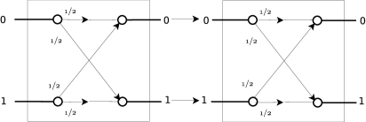
Figure 5.3: Conjunction of two $C$ gates. Internal line labels represent probabilities for transitions.

Let us now consider the effect of concatenating two instances of $C$ and two instances of $Q$, respectively. Transition probabilities for the former (see Figure 5.3) are:

$$p^{C_{1}C_{2}}_{00} =p^{C_{1}}_{00}\times p^{C_{2}}_{00}+p^{C_{1}}_{01}\times p^{C_{2}}_{10}$$

$$=p^{C_{1}C_{2}}_{01} =p^{C_{1}}_{01}\times p^{C_{2}}_{11}+p^{C_{1}}_{00}\times p^{C_{2}}_{01}$$

$$=p^{C_{1}C_{2}}_{10} =p^{C_{1}}_{10}\times p^{C_{2}}_{00}+p^{C_{1}}_{11}\times p^{C_{2}}_{10}$$

$$=p^{C_{1}C_{2}}_{11} =p^{C_{1}}_{10}\times p^{C_{2}}_{01}+p^{C_{1}}_{11}\times p^{C_{2}}_{11}$$

$$=1/4+1/4=1/2.$$ (5.3)

Transition probabilities for a concatenation of the two quantum gates, on the other hand, are:

$$p^{Q_{1}Q_{2}}_{00}=p^{Q_{1}Q_{2}}_{11}=0,$$

$$p^{Q_{1}Q_{2}}_{01}=p^{Q_{1}Q_{2}}_{10}=1.$$ (5.4)

In other words, these two quantum gates, which by themselves yield equal probabilities for each of the two possible outcomes, together yield an outcome that is anti-correlated with the input value with certainty. That this is so is evident if we consider, for example, the action of $Q_{1}$ and $Q_{2}$ on a qubit in the initial state $|0\rangle$:

$$|0\rangle\xrightarrow{Q_{1}}\frac{i}{\sqrt{2}}|0\rangle+\frac{1}{\sqrt{2}}|1\rangle$$

$$\xrightarrow{Q_{2}}\frac{i}{\sqrt{2}}\left(\frac{i}{\sqrt{2}}|0\rangle+\frac{1}{\sqrt{2}}|1\rangle\right)+\frac{1}{\sqrt{2}}\left(\frac{1}{\sqrt{2}}|0\rangle+\frac{i}{\sqrt{2}}|1\rangle\right).$$ (5.5)

This may be re-expressed as:

$$\left(\frac{i}{\sqrt{2}}\cdot\frac{i}{\sqrt{2}}+\frac{1}{\sqrt{2}}\cdot\frac{1}{\sqrt{2}}\right)|0\rangle+\left(\frac{i}{\sqrt{2}}\cdot\frac{1}{\sqrt{2}}+\frac{i}{\sqrt{2}}\cdot\frac{1}{\sqrt{2}}\right)|1\rangle.$$ (5.6)

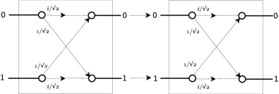
Figure 5.4: Conjunction of two $Q$ gates. Internal line labels represent probability amplitudes for transitions.

Eq. (5.6) illustrates the fact, visualised in Figure 5.4, that in order to derive the probability for the outcome of a particular quantum mechanical experiment we must first calculate the total probability amplitude corresponding to that particular outcome, by summing the probability amplitudes for all of the possible paths through the state space of the system which yield that particular result. Some of these paths may ‘interfere’ with one another. In the current example, the probability amplitudes for the two possible paths yielding $|0\rangle$ are $(i/\sqrt{2})^{2}=-1/2$ and $(1/\sqrt{2})^{2}=1/2$. Since these are of opposite sign, they destructively interfere with one another, yielding, in this case, a total probability amplitude of 0. The probability amplitudes for the two possible paths which yield $|1\rangle$, on the other hand, constructively interfere to yield a total probability amplitude of $i$. By the Born rule, the probability that the result is $|1\rangle$ is $|i^{2}|=1$. Similarly, the reader can verify that the action of the combined gate on an initial state of $|1\rangle$ will yield an outcome of $|0\rangle$ with certainty.

It is worthwhile to note, here, a fact which I did not call explicit attention to in my earlier exposition of the Deutsch-Jozsa algorithm: recall (cf. §2.2, n. 9.) that when the function encoded in the unitary transformation is balanced, the amplitude of $|0^{n}\rangle$ in the superposition (2.4) representing the first $n$ qubits, owing to destructive interference, will be zero. Thus a measurement of these qubits cannot produce the bit string $z=0$, and this fact allows us to distinguish constant functions, which always yield the bit string $z=0$, from balanced functions, which always result in a bit string $z\neq 0$. Indeed, based on such considerations, Lance Fortnow has gone so far as to claim that interference, in this sense, and not entanglement, is the true source of quantum speedup. We will not have to consider Fortnow’s claim in detail here (though the interested reader is encouraged to consult Appendix E), for as I will argue later, in §5.5 and §5.6, entanglement and interference can be considered as but two sides of one and the same coin.

5.4.2 The two-slit experiment

For Richard Feynman, the phenomenon (introduced in the last section) of ‘self-interference’, which we can more abstractly characterise as—a consequence of the superposition principle—the need to sum the probability amplitudes over all of the possible paths through a system’s state space, “has in it the heart of quantum mechanics. In reality, it contains the only mystery” (Feynman et al., 1964, vol. 3, 1-1). What makes this phenomenon so mysterious is the fact that classically, interference is typically associated exclusively with wave propagation, but many of the objects which exhibit interference effects in quantum mechanics also exhibit characteristically particle-like effects.

Consider, for instance, an experimental setup consisting of a classical wave source, a diaphragm into which two openings have been cut, and a movable (in the vertical direction) detector, arranged as in Figure 5.5. The detector measures the intensity of the wave motion at that location. We find that in general this intensity can take on a continuous range of values whose distribution for different positions of the detector reflects the constructive and destructive interference of the waves emanating from the apertures. Consider, on the other hand, a similarly arranged experimental setup with, in lieu of a classical wave source, a classical particle emitter (also depicted in Figure 5.5), which emits, one at a time, particles of identical shape and size in random directions. Since the particles are fired from the gun one at a time we will of course find no interference effects. As for the detector, it will either detect a particle or it will not, thus the distribution of intensity values will decidedly not be continuous.

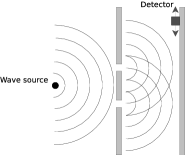
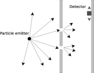
Figure 5.5: A two-slit experiment with, left: a classical wave source, and right: a classical particle emitter.

When we come to perform similarly arranged experiments with quantum objects, however, things begin to get more puzzling. For instance, suppose that, analogously to our experiment with the classical particle emitter, we set up an experimental apparatus consisting of a diaphragm with two apertures, a movable detector, and an electron gun. In this case we find that, on the one hand, as we would expect on the assumption that electrons are particles, they arrive at the detector one at a time and are registered with equal intensity. On the other hand, the probability that an electron will arrive at any given position on the back wall is distributed analogously to the intensity distribution for a classical wave—i.e., the probability distribution displays interference effects, as we saw in our comparison of classical and quantum computer gates above. Quantum objects like electrons, therefore, manifest both particle and wave effects.

This is extremely counter-intuitive. It is difficult if not impossible to imagine how particles, shot one at a time through a slitted diaphragm can interfere with one another. For Feynman, this phenomenon is simply a brute fact—one which “is impossible, absolutely impossible, to explain in any classical way” (1964, vol. 3, 1-1).

It is possible, of course, to account for these statistics by appealing to the formal requirement of which Eq. (5.6) is an example; however, Feynman does not consider such an account to be explanatory; for him it is only an account: “We cannot make the mystery [of self-interference] go away by ‘explaining’ how it works. We will just tell you how it works” (1964, vol. 3, 1-1). For Feynman, what is missing from such an account is precisely a causal or mechanistic description of the process by which self-interference phenomena arise. Feynman is of the opinion that explanations of physical phenomena should account for the mechanisms that give rise to them—something which he adamantly believes cannot be done in the case of self-interference phenomena:

One might still like to ask: “How does it work? What is the machinery behind the law?” No one has found any machinery behind the law. No one can “explain” any more than we have just “explained.” No one will give you any deeper representation of the situation. We have no ideas about a more basic mechanism from which these results can be deduced (1964, vol. 3, 1-10).

5.5 Accounting for correlations in EPRB composite systems

Consider two fermions (spin-1/2 systems) initially brought into interaction with one another to form a composite system with zero total spin in every direction. The system is said to be in the ‘singlet state’. Since fermions may only take on spin values of $\pm 1/2$, this requires that the spins of the individual subsystems be oppositely correlated with one another; i.e., the only possibilities for their respective spins are: (a) $1/2,-1/2$; (b) $-1/2,1/2$. Conservation of angular momentum dictates that as long as there are no further interactions, the subsystems must maintain their correlation with one another even if, after some elapsed time, they become spatially separated. In particular, if we perform, for instance, a $\sigma_{z}$ experiment on one subsystem and receive a positive result, then a $\sigma_{z}$ experiment on the second subsystem must yield a negative result with certainty, and vice versa. This will be the case regardless of the orientation of the experimental device; i.e., we have the following relation for the expectation value of experiments on the joint system for any direction $\hat{m}$:

$$\langle\sigma_{m}\otimes\sigma_{m}\rangle=-1.$$ (5.7)

On the other hand, if we perform a $\sigma_{z}$ experiment on the first system and a $\sigma_{x}$ experiment on the second we will find no correlation between the respective results. In general, for unit vectors $\hat{m},\hat{n}$:

$$\langle\sigma_{m}\otimes\sigma_{n}\rangle=-\hat{m}\cdot\hat{n},$$ (5.8)

where the scalar product $\hat{m}\cdot\hat{n}\equiv\lVert m\rVert\lVert n\rVert cos\theta=cos\theta$ for unit vectors $\hat{m},\hat{n}$. States such as the singlet state are examples of entangled states. As we have already discussed (§3.2.1, §4.3), there is no local hidden variables theory which can reproduce all of the predictions of quantum mechanics for states such as these.

Physically, entanglement is usually given a characterisation essentially similar to the one I have just given; i.e., when two (or more) quantum systems, existing independently of one another in different parts of space, are brought into temporary physical interaction to form a composite system, then if after a time the subsystems become spatially separated once again, it may happen that as a result of their interaction, probabilities for outcomes of experiments on the individual subsystems are no longer independent of one another. Once entered into, this situation will persist indefinitely and will only cease when the subsystems undergo further interactions with other (external) systems.

Key in the foregoing account are the ideas of spatially distinct quantum systems and of the physical interactions between them. Yet spatially separated ensembles are not the only quantum systems to display statistical dependence. The two-slit experiment with electrons, which we considered in §5.4.2, for instance, can be thought of as a series of experiments on a collection of identically prepared quantum systems which together comprise a temporally separated ensemble.

As we saw, the results of experiments on such systems may display statistical correlations with one another, which we normally conceive of as arising from self-interference. Self-interference, meanwhile, is typically considered to be an aspect of quantum mechanics that is fundamentally distinct from whatever gives rise to the statistical correlations observed in EPRB experiments (these, as we have just seen, are usually conceived of as being due to the physical interaction between spatially distinct subsystems).

According to John Stachel, however, quantum entanglement just is a species of statistical dependence, and is exhibited by both of these phenomena. Stachel attributes no special significance, in particular, to physical interactions between quantum systems: “Rather than a physical interaction, it is precisely the quantum entanglement of their members—non-interacting or interacting—that distinguishes quantum from classical ensembles” (1997, 246).

Ultimately, for Stachel, the statistical dependence observed in both cases is due to the requirement, illustrated by Eq. (5.6), that probability amplitudes for all of the possible paths through a system’s state space be summed in order to derive the probabilities for outcomes of experiments on that system. Let us call the collection of rules that encapsulate this requirement the ‘Feynman rules’ for short. We saw an example of how to apply these rules to single systems in §5.4.1. As for EPRB (and similar) systems composed of more than one subsystem, Stachel argues that one can think of experiments on such systems as composed of two steps. The first step, consisting of an experiment on the first subsystem, yields a non-maximal experimental outcome for the system as a whole. It is followed by an experiment on the second subsystem, which together with the first experiment can be considered as yielding a maximal experimental outcome for the total system. Given such a description of the experiment, Feynman’s rules can be shown to correctly account for the observed statistics.

5.6 Accounting for the Feynman rules

5.6.1 Physical interactions

In the last section we saw that it is possible to characterise the statistics manifested by EPRB-type composite systems as stemming from the need to sum the probability amplitudes for all of the paths a system may take through its state space (i.e., from Feynman’s rules). From this, Stachel has concluded that EPRB-type effects, usually taken as a paradigm example of the effects consequent upon physically interacting quantum systems, are in reality just consequences of Feynman’s rules. The requirement expressed by Feynman’s rules, in fact, for Stachel (just as for Feynman himself) is the true and only quantum mystery.

This would seem to undercut my claim that the explanation of quantum speedup I have given above can be construed in a causal way. But before we accept this conclusion, let us see if something rather more subtle may be at work. In particular, let us determine whether it is possible to characterise the requirements expressed by Feynman’s rules as themselves stemming from physical interactions of some sort. If we could show this, we might then conclude that characterising quantum systems in terms of the requirements imposed by Feynman’s rules, on the one hand, and in terms of physical interactions, on the other, are merely two different ways of regarding one and the same quantum mystery. Those with a predilection for causal-mechanical descriptions, of course, will prefer the latter.

In fact, we can provide such a characterisation if we focus on the system’s interaction with the state preparation device. In particular, the common source of fermions in the EPRB experiment may be taken to represent a physical source for the entanglement present in a system in (for instance) one of the Bell states—a physical source, moreover, that is in the common causal past of both subsystems.

That is all well and good for an experimental setup such as the EPRB. But, one might object, if we are to answer Stachel’s challenge we must provide a physical source for the entanglement present in temporal ensembles as well as in spatial ensembles, for the entanglement present in single particle experiments as well as in the EPRB-type experiments.

The following consideration should allay this concern. Imagine a spin-$\nicefrac{{1}}{{2}}$ particle that has been sent through a Stern-Gerlach apparatus oriented in the $\hat{z}$ direction (see Figure 5.6). Once it has passed through the apparatus, there is, henceforward, an important sense in which only joint experiments on the system are possible, for now an experiment to determine whether the particle occupies a particular spatial region is implicitly also an experiment to determine whether the particle is in a complementary spatial region. For supposing that the effect of the magnet is that the particle is now in a superposition of being in the spatial regions occupied by the $z+$ and $z-$ detectors. Then in that case the combined state of the two spatial regions will be expressible in the occupation number formalism (cf. Mattuck, 1976, Ch. 7) as follows:

$$|\psi\rangle=a|1\rangle_{z+}|0\rangle_{z-}+b|0\rangle_{z+}|1\rangle_{z-}.$$ (5.9)

Here, $|1\rangle_{\alpha}$ signifies that one particle occupies the spatial region inhabited by the $\alpha$ detector, while $|0\rangle_{\alpha}$ signifies that no particles occupy the spatial region inhabited by the $\alpha$ detector. Eq. (5.9) expresses the fact that if we perform a $\sigma_{z}$ experiment on $\psi$ and detect a particle at the $z+$ detector, then we cannot also detect a particle at the $z-$ detector, and vice versa. Thus we can think of the statistics associated with a single particle as, from another point of view, the statistics associated with an entangled state of two spatial regions, where this entangled state has been brought about via the influence of the Stern-Gerlach apparatus, which we can think of as representing “an influence on the very conditions which define the possible types of predictions regarding the future behaviour of the system” (Bohr, 1935, 700). In this vein one recalls Shimony: “It must be emphasized that the concept of entanglement is inseparable from the role of potentiality in quantum mechanics” (Shimony, 1993, 142-143). In an entangled state such as (5.9), Shimony writes, the two observables involved are “… merely potential, but in an interlocked manner” (ibid.).

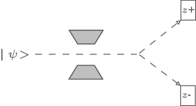
Figure 5.6: A Stern-Gerlach-like experimental setup (implementing a $\sigma_{z}$ experiment) in which a two-dimensional quantum system is sent through a state preparation device, after which it impinges on one of two detectors.

Considering the state of a system from varying points of view is all very well, one might interject at this point, but the proof is in the pudding: do such states manifest detectable correlations between their subsystems? The, perhaps surprising, answer seems to be yes; the state of a single system, such as a photon, can give rise to EPRB-type correlations that are detectable in principle by experiment. This was, in fact, illustrated with a gedankenexperiment, some time ago, by Lucien Hardy (1994). We will consider this gedankenexperiment in the next section.

5.6.2 Entanglement of a single photon

Hardy’s thought experiment consists of three 50:50 beam splitters each implementing the following state transformations, expressed in the occupation number formalism as:

$$|0\rangle_{a}|0\rangle_{b} \to|0\rangle_{c}|0\rangle_{d},$$ (5.10)

$$|0\rangle_{a}|1\rangle_{b} \to\frac{1}{\sqrt{2}}(|0\rangle_{c}|1|\rangle_{d}+i|1\rangle_{c}|0\rangle_{d}),$$ (5.11)

$$|1\rangle_{a}|0\rangle_{b} \to\frac{1}{\sqrt{2}}(i|0\rangle_{c}|1|\rangle_{d}+|1\rangle_{c}|0\rangle_{d}).$$ (5.12)

Here $a,b$ are the input and $c,d$ are the output modes, and it is assumed for simplicity that the $a$ mode is transmitted into the $c$ mode and likewise for $b$ and $d$. A photon, prepared in the state $q|0\rangle_{s}+r|1\rangle_{s}$, is directed at the $s$ input of one of the beam splitters (see Figure 5.7), while the input to $t$ is the vacuum state $|0\rangle_{t}$. The outputs of this splitter, $u_{1}$ and $u_{2}$, are fed as inputs to two further beam splitters, where they are each mixed with the coherent states $|\alpha_{1}\rangle_{a_{1}}$ and $|\alpha_{2}\rangle_{a_{2}}$. The outputs of these beam splitters, $c_{1},d_{1},c_{2},d_{2}$ are then fed to photon number detectors, $C_{1},D_{1},C_{2},D_{2}$. Additionally, two more detectors, $U_{1},U_{2}$, may be optionally inserted into the paths $u_{1},u_{2}$, respectively.

Figure 5.7: The experimental setup for Hardy’s gedankenexperiment. A photon in the state $q|0\rangle+r|1\rangle$ is incident on the $s$ mode; the vacuum state is incident on the $t$ mode; $|\alpha_{1}\rangle$ and $|\alpha_{2}\rangle$ are incident on the $a_{1}$ and $a_{2}$ modes, respectively. Source: Hardy (1994).

It turns out that (cf. Hardy, 1994) when neither $U_{1}$ nor $U_{2}$ are removed from paths $u_{1}$ and $u_{2}$, it is impossible for both $U_{1}$ and $U_{2}$ to register a photon; writing $X_{i}=n$ to indicate that $n$ photons were detected at detector $X_{i}$, we have:

$$U_{1}=1\mbox{ and }U_{2}=1\mbox{ never happens}.$$ (5.13)

When $U_{1}$ is removed, we have the result that:

$$\mbox{if }F_{1}=1\mbox{ then }U_{2}=1,$$ (5.14)

where we have written $F_{1}=1$ as shorthand for $C_{1}=0,D_{1}=1$. Similarly, when $U_{2}$ is removed:

$$\mbox{if }F_{2}=1\mbox{ then }U_{1}=1,$$ (5.15)

where $F_{2}=1$ is shorthand for $C_{2}=0,D_{2}=1$. When $U_{1}$ and $U_{2}$ are both removed, we find that

$$F_{1}=1\mbox{ and }F_{2}=1\mbox{ happens sometimes.}$$ (5.16)

To appreciate the significance of these results, imagine that Alice and Bob are at ends 1 and 2 respectively, and suppose that Alice chooses to perform experiment $F_{1}$ and Bob chooses to perform experiment $F_{2}$. Further suppose that these yield $F_{1}=1,F_{2}=1$. Alice can deduce from $F_{1}=1$ and (5.14) that the photon from the source would have been detected in $u_{2}$ if Bob had placed $U_{2}$ there. From $F_{2}=1$ and (5.15), Bob can deduce that the photon from the source would have been detected in $u_{1}$ if the detector $U_{1}$ had been placed there by Alice. They cannot both be correct, however, for only one photon has been emitted from the source; i.e., (5.13) will then be violated.

According to Hardy, it is possible to avoid this contradiction if we are willing to drop the assumption of locality:

… there is an implicit assumption of locality in this reasoning, and … without this assumption there is no contradiction. Alice obtains $F_{1}=1$. Bob is actually measuring $F_{2}$. Alice might deduce from her result and the prediction [(5.14)] that had Bob measured $U_{2}$ instead he would have gotten $U_{2}=1$. However, without assuming locality, this deduction is wrong, because if Bob had decided to measure $U_{2}$ instead, there might then have been a nonlocal influence from Bob’s end to Alice’s end (Hardy, 1994, 2281-2282).

Let us forego evaluating Hardy’s interpretation of the significance of this experiment (specifically, his attribution of nonlocality to the effects manifested by the experiment). It is enough to note that, irrespective of whether we interpret these effects as nonlocal, the Hardy gedankenexperiment manifests effects which we would normally associate with physically interacting multi-particle systems. The experiment thus illustrates, in a concrete manner, that the quantum superposition of a single system can also be thought of in terms of the correlations consequent upon its physical interactions with an experimental device. In this vein, Dunningham & Vedral (2007, 1) conclude:

Feynman once famously claimed that superposition is the only mystery in quantum mechanics. Others would add nonlocality to the list. If, however, single particles can exhibit nonlocality, then these two mysteries become one and the same.

Entanglement represents a real physical feature of quantum systems, whether or not we maintain that we should require of such physical features that they be explicable in terms of the physical interactions of systems. An explanation of quantum speedup, therefore, according to which it is entanglement which makes it possible for quantum systems to outperform their classical counterparts, is a physical explanation of quantum speedup on a reasonable interpretation of what it means for an explanation to be physical.

Chapter 6 Summary and Conclusion

section

In Chapter 2 I began this dissertation by considering the most popular of the candidate physical explanations for quantum speedup: the so-called many worlds explanation of quantum computation. I argued that, although it is inspired by the neo-Everettian interpretation of quantum mechanics, unlike the latter it does not have the conceptual resources required to overcome the preferred basis objection. I also argued that the many worlds explanation, at best, can serve as a good description of the physical process which takes place in network-based computation, but that it is incompatible in an important sense with other models of computation such as cluster state quantum computing. I next considered, in Chapter 3, a common component of most other candidate explanations of quantum speedup: quantum entanglement. I investigated whether entanglement can be said to be a necessary component of any explanation for quantum speedup, and I considered two major purported counter-examples to this claim. I argued that neither of these, in fact, show that entanglement is unnecessary for speedup, and that, on the contrary, we should conclude that it is. In Chapters 4 and 5 I then asked whether entanglement can be said to be sufficient as well. In Chapter 4 I argued that despite a result that seems to indicate the contrary, entanglement, considered as a resource, can be seen as sufficient to enable quantum speedup. Finally, in Chapter 5 I argued that entanglement is sufficient to explain quantum speedup.

In this dissertation I have neither proved any original theorems, nor provided any new experimental results. Rather, my conclusions are the result of an investigation and analysis of the valuable scientific contributions which have already been made. As compared to these, my own contribution is slight. But I hope that the reader agrees that it is not unimportant—that even if, for all of my efforts, my conclusions are in fact incorrect, that there has been some clarification of the underlying issues, with the hoped-for result that there will, in the not too distant future, be new theorems and new results in the directions pointed to by this dissertation.

In his closing remarks to the Logical Syntax of Language, Carnap wrote of a vision of “fruitful co-operative work on the part of the various investigators working on the same problems—work fruitful for the individual questions of the logic of science, for the scientific domain which is being investigated, and for science as a whole.” For ‘logic of science’ I would put, in its place, ‘philosophy of science’. But I wholeheartedly agree with the spirit of these words. And it is my sincere hope that this dissertation makes some approximation to this so eloquently expressed ideal.

Appendix A Computational complexity theory

chapter

Alan Turing (1937; 1938) inaugurated the field of Computer Science by arguing persuasively for the equivalence of the class of computable, or ‘effectively calculable’ functions with the class of problems computable by a Turing machine. The statement of this equivalence is known as the Church-Turing thesis, and it is the fundamental principle of computer science. In its early period, research in computer science was focused primarily on the question of computability; i.e., on the question of whether a given problem is or is not computable by Turing machine. More recently, another focus of research has emerged: the field known as Computational Complexity Theory. This field is dedicated to the more practical question concerning the cost of solving a given computational problem.

A basic distinction, in Complexity Theory, is between those computational problems that are amenable to an efficient solution in terms of time and/or space resources, and those that are not. Easy (or ‘tractable’, ‘feasible’, ‘efficiently solvable’, etc.) problems are those for which solutions exist which involve resources bounded by a polynomial in the input size, $n$. Hard problems are those which are not easy, i.e., they are those whose solution requires resources that are ‘exponential’ in $n$, i.e., that grow faster than any polynomial in $n$ (Nielsen & Chuang, 2000, p. 139).

For example, a problem, which for input size $n$, requires $\approx n^{c}$ steps to solve (where $c$ is some constant) is polynomial in terms of time resources in $n$ and thus tractable according to our definition. A problem that requires $\approx c^{n}$ steps to solve, on the other hand, is exponential in terms of time resources in $n$ and is therefore intractable according to our definition. The definition is a coarse one, and its usefulness will depend, in a given case, on the values of $c$ and $n$. Nevertheless it is adequate for most cases of practical interest.

An important theoretical reason for adopting the definition is the following principle, usually referred to as the ‘Strong’ Church-Turing thesis in the literature. In order not to confuse this thesis with the more fundamental (‘weak’) Church-Turing thesis that I mentioned earlier, I will refer to it as the Computational Efficiency Thesis (CET), which states that:

Any model of computation can be simulated on a probabilistic Turing machine with at most a polynomial increase in the number of elementary operations required (Nielsen & Chuang, 2000, p. 140).

If, now, we identify easy problems with those having polynomial resource solutions, then CET tells us that in our analysis of computational complexity, we can restrict our attention to the probabilistic Turing machine model of computation (Nielsen & Chuang, 2000, p. 140). Our definition of an easy problem, coupled with the CET, thus provides us with an elegant, model-independent theory of computational complexity. But note that while CET is what gives computational complexity theory its elegant model-independent character, and that without it “computational concepts and even computational kinds such as ‘an efficient algorithm’ or ‘the class NP’ will become machine-dependent, and recourse to ‘hardware’ will become inevitable in any analysis of the notion of computational complexity” (Hagar, 2007, p. 245), it is not a foundational principle to the field of computational complexity theory in the same way that the Church-Turing thesis is to computer science.

Problems that are decidable in polynomial time by a deterministic Turing machine are said to be in the complexity class PTIME, usually referred to simply as P. Problems for which a deterministic Turing machine can verify whether a given solution is, in fact, a solution are said to be in the complexity class NP. For example, consider a language $L=\{10,11,101,111,1011,...\}$ over the alphabet $\Sigma=\{0,1\}$, the set of binary digits. $L$ is the set of binary representations of prime numbers. If it is possible for a deterministic Turing machine to decide, using only polynomial time resources, whether an arbitrary binary input string is in the language (i.e., whether it is a prime number), we say the problem is in P. If, on the other hand, one is given a string in the language at the outset, then if it is possible for a deterministic Turing machine to verify, in polynomial time, that the string is, in fact, in the language, then the problem is said to be in NP.

A long-standing question in complexity theory is the nature of the relationship between P and NP. P is clearly a subset of NP. If it can be decided in polynomial time whether an arbitrary string is a member of $L$, then, trivially, it can be decided in polynomial time whether a member of $L$ is a member of $L$. It is strongly suspected that P is a proper subset of NP, however this has not yet been proven. This is known as the P $\neq$ NP problem in complexity theory.

An important notion in complexity theory is reducibility. Intuitively, problem $B$ is reducible to problem $A$ if, with no more than polynomial overhead, we can convert an algorithm for deciding $B$ into an algorithm for deciding $A$. In other words, $B$ is reducible to $A$ if a solution for $A$ can be used to solve $B$. Reducibility leads us to our next important complexity class, NP-complete. A problem, $C$, is called NP-complete if $C$ is in NP and every other problem in NP is reducible (in polynomial time) to $C$. The concept of an NP-complete problem is important for the resolution of the P $\neq$ NP problem, for if it can be shown that an NP-complete problem is solvable in polynomial time by a deterministic Turing machine (i.e., if it can be shown that it is in P), then it follows that all other problems in NP are also in P, and hence that P = NP.

Besides P and NP, the two most relevant complexity classes with respect to quantum computation are BPP and BQP. BPP stands for bounded-error probabilistic time. A problem, $A$, is in BPP if there is a (classical) probabilistic Turing machine that will accept a string $x$ with probability $1/2\leq k\leq 1$ if $x\in L$ (the language representing $A$) and reject it with probability $1/2\leq k\leq 1$ if $x\notin L$ (Nielsen & Chuang, 2000, p. 152-153). The quantum analogue of BPP is BQP (bounded error quantum polynomial time), the set of problems such that a quantum computer will accept $x$ with probability $1/2\leq k\leq 1$ if $x\in L$ and reject $x$ with probability $1/2\leq k\leq 1$ if $x\notin L$ (Nielsen & Chuang, 2000, pp. 200-202). BPP $\subseteq$ BQP since a quantum computer can efficiently simulate a classical probabilistic Turing machine (Nielsen & Chuang 2000, p. 30; Hagar 2007, p. 240). However, it is not clear whether BQP $\neq$ BPP.

It is important to note that proving BQP $\neq$ BPP amounts to proving that quantum computers are more powerful than classical computers; but while it is strongly suspected that BQP $\neq$ BPP, this question has not yet been resolved. Factoring, the most famous problem for which a quantum algorithm has been developed, has not been proven to be outside P. Thus solving the factoring problem does not show us that P $\neq$ BQP, let alone that BPP $\neq$ BQP. Note also that as of yet no quantum algorithm has been developed which can efficiently solve a problem inside the class NP-complete, and the relation between NP and BQP is still unknown.

For more on computational complexity, see: Papadimitriou (1994), Nielsen & Chuang (2000), Aaronson (2012).

Appendix B Information Theory

B.1 Shannon entropy

The birth and development of classical information theory is due, in large part, to the pioneering work of Claude Shannon. In his seminal article, “A Mathematical Theory of Communication” (1948), Shannon introduced the scientific community to the fundamental information-theoretic concept of entropy. Entropy is a measure of the information one gains when one comes to know the value of a random variable. Equivalently, it can be thought of as the uncertainty associated with a random variable; e.g., a message produced by an information source. We define the Shannon entropy, $H$, with respect to the random variable $x$, as:

$$H(x)=-K\sum_{i=1}^{n}p(x_{i})\log p(x_{i}),$$ (B.1)

where $K$ is a positive constant (amounting to a choice of unit measure) normally chosen to be 1 (Shannon, 1948, p. 11), $0\log 0$ is conventionally defined to be 0, and $p(x_{i})$ refers to the probability of receiving message $i$, given a set of $n$ possible messages. The $\log$ is typically taken to base 2. For example, suppose an information source transmits sequences of binary digits with the probabilities of the next digit in the sequence being a 0 or a 1, $1/3$ and $2/3$, respectively. In this case our uncertainty with respect to the next bit, or our entropy, is $-(1/3\times\log 1/3+2/3\times\log 2/3)=0.92.$

Considered as a measure of our uncertainty with respect to the messages produced by an information source, we should expect $H$ to be 0 if we are certain of the result, i.e., if one of the $p(x_{i})=1$. It is easily verified that this is the case. We should also expect $H$ to be at a maximum when the bits are received with equal probability, for this is the situation in which we are most uncertain of the result. This is also easily verified (cf. Shannon, 1948, p. 11).

The joint entropy of two random events, $x$ and $y$ is the total uncertainty associated with $x$ and $y$. To determine it one must take into account the probabilities of all possible combinations of values for $x$ and $y$. Thus,

$$H(x,y)=-\sum_{i,j}p(x_{i},y_{j})\log p(x_{i},y_{j}).$$ (B.2)

Here, $p(x_{i},y_{j})$ refers to the probability that message $x_{i}$ and $y_{j}$ occur together.

Note that it can be shown that $H(x,y)\leq H(x)+H(y)$, with equality only if the events $x_{i}$ and $y_{j}$ are independent. This is called subadditivity (intuitively, the total uncertainty associated with $x$ and $y$ is equal to the sum of the uncertainties of $x$ and $y$ unless they share information in common). Strong subadditivity, $H(x,y,z)\leq H(x,y)+H(y,z)-H(y),$ also holds for the Shannon entropy.

The conditional entropy of $x$ with respect to $y$,

$$H(x|y)=H(x,y)-H(y),$$ (B.3)

is the total uncertainty associated with $x$ and $y$ minus the uncertainty that disappears once we come to know $y$.

The information shared in common between $x$ and $y$, or mutual information of $x$ and $y$ is defined as

$$H(x:y)=H(x)+H(y)-H(x,y).$$ (B.4)

This definition is easily grasped if one expresses the equation in terms of the joint information, i.e., $H(x,y)=H(x)+H(y)-H(x:y),$ which is the total information gain associated with $x$ and $y$ minus the information shared in common (to avoid double counting) (Nielsen & Chuang, 2000, p. 506).

B.2 Von Neumann entropy

The von Neumann entropy plays the same role in quantum information theory as the Shannon entropy plays in classical information theory. It is defined as

$$S(\rho)=-\mbox{tr}(\rho\log\rho),$$ (B.5)

for a quantum system represented by the density matrix, $\rho$. As before, by convention, $0\log 0\equiv 0$. Since the trace of a matrix $A$ is equal to the sum of its eigenvalues; i.e., since $\mbox{tr}(A)=\sum\lambda_{i}$; the von Neumann entropy can be more usefully expressed as

$$S(\rho)=-\sum_{x}\lambda_{x}\log\lambda_{x}$$ (B.6)

where $\lambda_{x}$ are the eigenvalues of $\rho$.

The joint entropy of a state with two components $A$ and $B$ is defined as

$$S(A,B)=-\mbox{tr}(\rho^{AB}\log(\rho^{AB})),$$ (B.7)

where $\rho^{AB}$ is the density matrix of the composite system $AB$ (Nielsen & Chuang, 2000, p. 514).

Conditional entropy and mutual information are defined analogously to their classical counterparts. The conditional entropy is given by

$$S(A|B)=S(A,B)-S(B).$$ (B.8)

The mutual information is given by

$$S(A:B)=S(A)+S(B)-S(A,B).$$ (B.9)

There are interesting disanalogies between the von Neumann and the Shannon entropy. For instance, the inequality $S(A)\leq S(A,B)$ does not hold in quantum information theory, as it does for the classical case. In the classical case it is intuitively obvious that the uncertainty associated with the state of one random variable cannot be more than the uncertainty associated with the joint state of two. But in the quantum case, this relation will fail to hold, for instance, in the case where we have a maximally entangled state of two subsystems. In this case, the joint state of the two systems is pure, and hence $S(A,B)=0$, but the marginals are completely mixed and thus $S(A)=S(B)=1.$ One other disanalogy, between the classical and quantum versions of mutual information, is discussed in greater detail in Chapter 3.

Appendix C Quantum teleportation

One of the most well-known applications of entanglement in quantum information processing is as a resource in the so-called teleportation protocol (cf. Nielsen & Chuang, 2000; Mermin, 2007). Consider Alice and Bob, two spatially separated experimenters, who have the ability to send classical information to one another (e.g., Alice may call Bob on the telephone, send him an email, and so on). Imagine that Alice would like to send the state (which she does not know) of some arbitrary qubit, $|\psi\rangle=\alpha|0\rangle+\beta|1\rangle$, to Bob. Classically, this seems like a very difficult task, for even if Alice knows the state of the qubit, she seems, in principle, to require an infinite amount of classical information to describe it precisely, for the state of a qubit will in general take on a continuum of values.

But suppose that Alice and Bob are given one extra resource: suppose that the Bell state $|\Phi^{+}\rangle$ is generated, and that one half of the Bell pair is given to Bob and the other half to Alice. Alice may now proceed as follows. First, she interacts the qubit represented by $|\psi\rangle$, whose state she wishes to send to Bob, with the Bell pair; i.e.,

$$|\psi\rangle_{a}|\Phi^{+}\rangle_{ab}=\frac{1}{\sqrt{2}}[\alpha|0\rangle_{a}(|00\rangle+|11\rangle)_{ab}+\beta|1\rangle_{a}(|00\rangle+|11\rangle)_{ab}],$$

where $a$ and $b$ indicate whether the qubits are in Alice’s or Bob’s possession. Alice then applies a controlled-not (CNOT) operation to the qubits in her possession, using the qubit represented by $|\psi\rangle$ as the control and her member of the Bell pair as the target qubit. This results in:

$$\frac{1}{\sqrt{2}}[\alpha|0\rangle_{a}(|00\rangle+|11\rangle)_{ab}+\beta|1\rangle_{a}(|10\rangle+|01\rangle)_{ab}].$$

Now Alice sends the qubit represented by $|\psi\rangle$ through a Hadamard gate, which results in:

$$\frac{1}{2}[\alpha(|0\rangle+|1\rangle)_{a}(|00\rangle+|11\rangle)_{ab}+\beta(|0\rangle-|1\rangle)_{a}(|10\rangle+|01\rangle)_{ab}]$$

$$=\frac{1}{2}[|00\rangle_{aa}(\alpha|0\rangle+\beta|1\rangle)_{b}+|01\rangle_{aa}(\alpha|1\rangle+\beta|0\rangle)_{b}$$

$$+|10\rangle_{aa}(\alpha|0\rangle-\beta|1\rangle)_{b}+|11\rangle_{aa}(\alpha|1\rangle-\beta|0\rangle)_{b}].$$

In the next step, Alice measures her two qubits. This will yield one of four possible measurement results (00, 01, 10, 11), and Bob’s qubit will correspondingly be in one of the following four states:

$$00:\quad |\psi\rangle_{b}\equiv(\alpha|0\rangle+\beta|1\rangle)_{b}$$

$$01:\quad |\psi^{\prime}\rangle_{b}\equiv(\alpha|1\rangle+\beta|0\rangle)_{b}$$

$$10:\quad |\psi^{\prime\prime}\rangle_{b}\equiv(\alpha|0\rangle-\beta|1\rangle)_{b}$$

$$11:\quad |\psi^{\prime\prime\prime}\rangle_{b}\equiv(\alpha|1\rangle-\beta|0\rangle)_{b}$$

Alice now communicates her result to Bob using a classical communications link (e.g. a telephone line). If Alice’s result is 00, then Bob’s state is $|\psi\rangle_{b}=\alpha|0\rangle+\beta|1\rangle=|\psi\rangle_{a}$, i.e., the state that Alice had originally intended to transfer. Otherwise, Bob can apply a unitary transformation to his qubit which will transform it into the state $|\psi\rangle_{b}$. For instance, if Alice’s result is 01, Bob will apply the Pauli X transformation. Recalling that $|0\rangle\equiv\left(\begin{smallmatrix}1\\ 0\end{smallmatrix}\right)$ and $|1\rangle\equiv\left(\begin{smallmatrix}0\\ 1\end{smallmatrix}\right)$, we see that

$$\mathbf{X}|\psi^{\prime}\rangle_{b}=\left(\begin{matrix}0&1\\ 1&0\end{matrix}\right)\left[\beta\left(\begin{matrix}1\\ 0\end{matrix}\right)+\alpha\left(\begin{matrix}0\\ 1\end{matrix}\right)\right]=\left(\begin{matrix}0&1\\ 1&0\end{matrix}\right)\left(\begin{matrix}\beta\\ \alpha\end{matrix}\right)=\left(\begin{matrix}\alpha\\ \beta\end{matrix}\right)=|\psi\rangle_{b}.$$

If Alice’s result is 10, then Bob applies a Pauli Z transformation:

$$\mathbf{Z}|\psi^{\prime\prime}\rangle_{b}=\left(\begin{matrix}1&0\\ 0&-1\end{matrix}\right)\left[\alpha\left(\begin{matrix}1\\ 0\end{matrix}\right)-\beta\left(\begin{matrix}0\\ 1\end{matrix}\right)\right]=\left(\begin{matrix}1&0\\ 0&-1\end{matrix}\right)\left(\begin{matrix}\alpha\\ -\beta\end{matrix}\right)=\left(\begin{matrix}\alpha\\ \beta\end{matrix}\right)=|\psi\rangle_{b}.$$

Finally, if Alice’s result is 11, then the reader can verify that Bob should apply the combined transformation ZX.

Figure C.1: A quantum circuit for the teleportation of a qubit. The top two lines represent the parts of the system accessible to Alice; the bottom line is the part of the system accessible to Bob.

Appendix D Separable operations

chapter

An open quantum system (e.g., a noisy quantum circuit) is one in which the state changes of the system of interest, $S$, are due both to its own internal dynamics and to its interaction with an external environment or ‘reservoir’, $R$. Let the initial state of the overall system be the product state, $\rho\otimes\omega_{R}$, with $\rho\in\mathcal{H}_{S}$, $\omega_{R}\in\mathcal{H}_{R}$ where $\mathcal{H}_{S},\mathcal{H}_{R}$ are the Hilbert spaces associated with $S$ and $R$. Then a state change of $S$ can be expressed as:

$$\rho\mapsto\Lambda\rho=\mbox{tr}_{R}(U\rho\otimes\omega_{R}U^{\dagger}),$$ (D.1)

where $\Lambda$ is the dynamical transformation map for $S$ which maps density operators to density operators, $U\equiv e^{-iH_{S+R}t/\hbar}$ is the time evolution operator for the combined system, and $\mbox{tr}_{R}$ is the partial trace over $R$.

For many purposes it is more convenient to express $\Lambda$ exclusively in terms of $S$. Take $|f_{\nu}\rangle$ to be an orthonormal basis for the state space of the reservoir (which we assume, without loss of generality, to be pure), with $\omega_{R}=|f_{0}\rangle\langle f_{0}|$ the reservoir’s initial state. Since the partial trace, over $R$, of $\rho\otimes\omega_{R}$ is given by $\mbox{tr}_{R}(\rho\otimes\omega_{R})=\langle f_{\nu}|\rho\otimes\omega_{R}|f_{\nu}\rangle$, we can rewrite (D.1) as:

$$\rho\to\Lambda\rho =\sum_{\nu}\langle f_{\nu}|U\big{[}\rho\otimes|f_{0}\rangle\langle f_{0}|\big{]}U^{\dagger}|f_{\nu}\rangle$$

$$=\sum_{\alpha}E_{\alpha}\rho E_{\alpha}^{\dagger},$$ (D.2)

where $E_{\alpha}\equiv\langle f_{\nu}|U|f_{0}\rangle$ is an operator on the state space of $S$, and the $E_{\alpha}$, known as Kraus operators or operation elements, satisfy the completeness relation:

$$\sum_{\alpha}E_{\alpha}^{\dagger}E_{\alpha}=I.$$ (D.3)

Separable operations are those operations that can be decomposed as a product of Kraus operators as follows:

$$\Lambda\rho=\sum_{k}A_{k}\otimes B_{k}\rho A^{\dagger}_{k}\otimes B^{\dagger}_{k}$$ (D.4)

such that $\sum_{k}A^{\dagger}_{k}A_{k}\otimes B^{\dagger}_{k}B_{k}=\mathbf{1}\otimes\mathbf{1}$.

If Alice and Bob perform only LOCC (‘local operations plus classical communications’) operations on a shared system $\rho$, then their individual Kraus operators may be joined together into product Kraus operators; i.e., into the form of a separable operation. The converse is false (Bennett et al., 1999). Separable operations are nevertheless a convenient proxy for LOCC operations, as the optimal implementation, via separable operations, of a given task provides strong bounds for what can be achieved using LOCC (see, for instance, Rains 2001; Virmani & Plenio 2003).

Appendix E Lance Fortnow’s Matrix Framework

Let us first consider a classical nondeterministic Turing machine. We begin by defining the transition function, $\delta$, of the machine in terms of a transition matrix, such that there is an entry in the matrix corresponding to every possible transition of the machine. We allow matrix entries to contain arbitrary nonnegative rational numbers. We then define the matrix entry, $T(c_{a},c_{b}),$ as the probability that the computer goes to configuration $c_{b}$ from configuration $c_{a}$ in one computational step. $T^{r}(c_{a},c_{b}),$ correspondingly, is the probability of getting to $c_{b}$ from $c_{a}$ in $r$ steps; it is the sum of the probabilities of each computational path of length $r$ leading from $c_{a}$ to $c_{b}$, with the restriction that the sum of all possible computational paths of length $r$ beginning from $c_{a}=1$.

$$\begin{matrix}&c_{a}&c_{b}&c_{c}&c_{d}&c_{e}&c_{f}&c_{g}&c_{h}\\ c_{a}&0.0&0.2&0.3&0.5&0.0&0.0&0.0&0.0\\ c_{b}&0.0&0.0&0.0&0.5&0.0&0.0&0.0&0.5\\ c_{c}&0.0&0.0&0.0&0.5&0.0&0.0&0.5&0.0\\ c_{d}&0.0&0.0&0.0&0.0&0.6&0.4&0.0&0.0\\ c_{e}&0.0&0.0&0.0&0.0&1.0&0.0&0.0&0.0\\ c_{f}&0.0&0.0&0.0&0.0&0.0&1.0&0.0&0.0\\ c_{g}&0.0&0.0&0.0&0.0&0.0&0.0&1.0&0.0\\ c_{h}&0.0&0.0&0.0&0.0&0.0&0.0&0.0&1.0\end{matrix}$$

Table E.1: A sample state transition matrix. Entries represent probabilities of transition between states.

Figure E.1: State diagram representation of the transition matrix in Table E.1. The edge labels represent the probability of a transition between the states connected by that edge.

For instance, given the matrix in Table E.1, we can determine that

$$T^{3}(c_{a},c_{e}) = [T(c_{a},c_{b})\times T(c_{b},c_{d})\times T(c_{d},c_{e})]+$$

$$[T(c_{a},c_{c})\times T(c_{c},c_{d})\times T(c_{d},c_{e})]$$

$$= (0.2\times 0.5\times 0.6)+(0.3\times 0.5\times 0.6)=0.15.$$

We can now define $T^{t}(c_{a},c_{f})$ as the probability of success for our nondeterministic Turing machine ($c_{a}$ and $c_{f}$ are the initial and accepting states, respectively) in $t$ time steps. It can be shown that a language $L$ is in the computational complexity class associated with classical probabilistic computation (BPP) if there is a probabilistic matrix $T$ such that, for $x\in L$ and $1/2\leq k\leq 1$ (typically taken to be 2/3),

$$T^{t}(c_{a},c_{f})\geq k,$$

and for $x\notin L$,

$$T^{t}(c_{a},c_{f})\leq k,$$

for polynomial $t$.

To capture the case of the quantum nondeterministic Turing machine, we omit the restriction that the matrix entries be nonnegative, and we redefine the probability of acceptance as $(T^{t}(c_{1},c_{A}))^{2}.$ It can be shown that a language $L$ is in the computational complexity class associated with quantum computation (BQP) if there is a matrix $T$, as just defined, such that, for $x\in L$,

$$(T^{t}(c_{a},c_{f}))^{2}\geq k,$$

and for $x\notin L$,

$$(T^{t}(c_{a},c_{f}))^{2}\leq k,$$

for polynomial $t$.

According to Fortnow, the fundamental difference between quantum and classical computing is interference. The matrix framework, according to Fortnow, shows us that, in a quantum computer, ‘bad’ computational paths are associated with negative matrix entries, allowing other computational paths to occur with higher probability. Fortnow writes: “The strength of quantum computing lies in the ability to have bad computation paths eliminate each other thus causing some good paths to occur with larger probability” (Fortnow, 2003, pp. 605-606).

Appendix F Spekkens vs. Quantum Transformations

In Robert Spekkens’ toy theory (2007), a system consists of a ball that can be in one of four boxes. A state, in the theory, is an expression of our knowledge of the location of the ball. For instance, if we know that the ball is in either the first or the second box, we write $1\lor 2$. Knowledge is restricted in the Spekkens theory. Aside from the ‘completely mixed state’, $1\lor 2\lor 3\lor 4$, the only other allowable states are the following six states of maximal knowledge:

$$\equiv 1\lor 2\equiv|0\rangle z+$$ ()

$$\equiv 3\lor 4\equiv|1\rangle z-$$ ()

$$\equiv 1\lor 3\equiv|+\rangle x+$$ ()

$$\equiv 2\lor 4\equiv|-\rangle x-$$ ()

$$\equiv 2\lor 3\equiv|+i\rangle y+$$ ()

$$\equiv 1\lor 4\equiv|-i\rangle y-$$ ()

Transformations of the Spekkens states are just permutations of the boxes. For instance, if we subject the state $1\lor 2$ to the permutation $\langle 1\rightarrow 2\rightarrow 3\rightarrow 1\rangle,$ the resulting state will be $2\lor 3$. Subjecting $3\lor 4$ to this permutation will result in $1\lor 4$.

We can associate some of the permutations of boxes in Spekkens’ toy theory with rotations of the Bloch sphere in quantum theory (Myrvold, 2010). In quantum theory, a $2\pi/3$ rotation of the Bloch sphere about the direction of $\hat{x}+\hat{y}+\hat{z}$ takes $x+\rightarrow y+$, $y+\rightarrow z+$, and $z+\rightarrow x+.$ In the Spekkens toy theory, this corresponds to the permutation $\langle 1\rightarrow 3\rightarrow 2\rightarrow 1\rangle$. Let us call this transformation $T_{1}$. A $\pi/2$ rotation of the Bloch sphere about the $z$-axis, in quantum theory, leaves $z+$ invariant but takes $x+$ to $y+$ and $y+$ to $x-$. Let us call this transformation $T_{2}^{q}$. It cannot be achieved in the Spekkens theory. An alternative, however, is a $\pi/2$ rotation about the $z$-axis followed by a reflection in the $xy$ plane, which corresponds, in the Spekkens theory to $\langle 1\rightarrow 3\rightarrow 2\rightarrow 4\rightarrow 1\rangle$. Call this transformation $T_{2}^{S}$. Note that while $T_{2}^{q}$ leaves $z+$ invariant, $T_{2}^{S}$ takes $z+$ to $z-$. It can be shown that the sets $\{T_{1},T_{2}^{q}\}$ and $\{T_{1},T_{2}^{S}\}$ are sufficient to generate the Spekkens and quantum groups of transformations, respectively.

Spekkens’s toy theory contains entangled states, but because of the differences in the allowable transformations between the toy theory and quantum theory, the set of entangled states that the toy theory contains is not identical to the set of entangled states contained in quantum theory; specifically, none of the entangled states in Spekkens’s toy theory yield correlations between outcomes of experiments that violate the Bell inequalities.

Vita

Name:	Michael E. Cuffaro
Post-Secondary	Concordia University
Education and	Montréal, Québec, Canada
Degrees:	1993–1994, 1997–2000 B.CompSc.
	Concordia University
	Montréal, Québec, Canada
	2007–2008 M.A.
	The University of Western Ontario
	London, Ontario, Canada
	2008–2013 Ph.D.
Honours and	Province of Ontario Graduate Scholarship
Awards:	2010–2011, 2011–2012, 2012–2013
	University of Western Ontario Graduate Teaching
	Assistantship Research Grant
	Fall 2009
Related Work	Instructor
Experience:	The University of Western Ontario
	Winter 2011, Winter 2013
	Teaching Assistant
	The University of Western Ontario
	2008–2010
	Teaching Assistant
	Concordia University
	2007–2008

Publications:

Cuffaro, M. (2012a). Many Worlds, the Cluster-state Quantum Computer, and the Problem of the Preferred Basis. Studies in History and Philosophy of Modern Physics, 43, 35-42.

Cuffaro, M. (2012b). Kant and Frege on Existence and the Ontological Argument. History of Philosophy Quarterly, 29, 337-354.

Cuffaro, M. (2012c). Kant’s Views on Non-Euclidean Geometry. To appear in the Proceedings of the Canadian Society for History and Philosophy of Mathematics.

Cuffaro, M. & Myrvold, W. (2012). On the Debate Concerning the Proper Characterisation of Quantum Dynamical Evolution. Accepted for publication in Philosophy of Science.

Muldoon, R., Borgida, M., & Cuffaro, M. (2012) The Conditions of Tolerance. Politics, Philosophy and Economics, 11, 322-344.

Cuffaro, M. (2011). On Thomas Hobbes’s Fallible Natural Law Theory. History of Philosophy Quarterly, 28, 175-190.

Cuffaro, M. (2010a). The Kantian Framework of Complementarity. Studies in History and Philosophy of Modern Physics, 41, 309-317.

Cuffaro, M. (2010b). Wittgenstein on Prior Probabilities. Proceedings of the Canadian Society for History and Philosophy of Mathematics, 23, 85-98.

Cuffaro, M. (2008). Nativist Models of the Mind. GNOSIS, 9.3.

Cuffaro, M. (2007). Which Rights are Basic Rights? GNOSIS, 9.1.

References

- Aaronson (2012) Aaronson, S. (2012). Complexity zoo. Qwiki: http://qwiki.stanford.edu/index.php/Complexity˙Zoo.
- Abbott (2012) Abbott, A. A. (2012). The Deutsch-Jozsa problem: De-quantisation and entanglement. Natural Computing, 11, 3–11.
- Albert & Loewer (1988) Albert, D., & Loewer, B. (1988). Interpreting the many worlds interpretation. Synthese, 77, 195–213.
- Barrett (2011) Barrett, J. (2011). Everett’s relative-state formulation of quantum mechanics. In E. N. Zalta (Ed.) The Stanford Encyclopedia of Philosophy. Spring 2011 ed.
- Bell (2004 [1964]) Bell, J. S. (2004 [1964]). On the Einstein-Podolsky-Rosen paradox. In Speakable and Unspeakable in Quantum Mechanics, (pp. 15–21). Cambridge: Cambridge University Press.
- Bell (2004 [1981]) Bell, J. S. (2004 [1981]). Bertlmann’s socks and the nature of reality. In Speakable and Unspeakable in Quantum Mechanics, (pp. 139–158). Cambridge: Cambridge University Press.
- Bennett et al. (1996) Bennett, C. H., Bernstein, H. J., Popescu, S., & Schumacher, B. (1996). Concentrating partial entanglement by local operations. Physical Review A, 53, 2046–2052.
- Bennett et al. (1993) Bennett, C. H., Brassard, G., Crépeau, C., Jozsa, R., Peres, A., & Wootters, W. K. (1993). Teleporting an unknown quantum state via dual classical and Einstein-Podolsky-Rosen channels. Physical Review Letters, 70, 1895–1899.
- Bennett et al. (1999) Bennett, C. H., DiVincenzo, D. P., Fuchs, C. A., Mor, T., Rains, E., Shor, P. W., Smolin, J. A., & Wootters, W. K. (1999). Quantum nonlocality without entanglement. Physical Review A, 59, 1070–1091.
- Biham et al. (2004) Biham, E., Brassard, G., Kenigsberg, D., & Mor, T. (2004). Quantum computing without entanglement. Theoretical Computer Science, 320, 15–33.
- Bohm (1951) Bohm, D. (1951). Quantum Theory. New York: Prentice Hall.
- Bohr (1935) Bohr, N. (1935). Can quantum-mechanical description of physical reality be considered complete? Physical Review, 48, 696–702.
- Braunstein et al. (1999) Braunstein, S. L., Caves, C. M., Jozsa, R., Linden, N., Popescu, S., & Schack, R. (1999). Separability of very noisy mixed states and implications for NMR quantum computing. Physical Review Letters, 83, 1054–1057.
- Braunstein & Pati (2002) Braunstein, S. L., & Pati, A. K. (2002). Speed-up and entanglement in quantum searching. Quantum Information & Computation, 2, 399–409.
- Brodutch & Terno (2011) Brodutch, A., & Terno, D. R. (2011). Entanglement, discord and the power of quantum computation. Physical Review A, 83, 010301.
- Bromberger (1966) Bromberger, S. (1966). Why questions. In R. G. Colodny (Ed.) Mind and Cosmos, (pp. 86–111). Pittsburgh: University of Pittsburgh Press.
- Bub (1977) Bub, J. (1977). Von Neumann’s projection postulate as a probability conditionalization rule in quantum mechanics. Journal of Philosophical Logic, 6, 381–390.
- Bub (2006) Bub, J. (2006). Quantum computation from a quantum logical perspective. arXiv:quant-ph/0605243v2.
- Bub (2010) Bub, J. (2010). Quantum computation: Where does the speed-up come from? In A. Bokulich, & G. Jaeger (Eds.) Philosophy of Quantum Information and Entanglement, (pp. 231–246). Cambridge: Cambridge University Press.
- Butterfield (2002) Butterfield, J. (2002). Some worlds of quantum theory. In R. J. Russell, P. Clayton, K. W. McNelly, & J. Polkinghorne (Eds.) Quantum Mechanics (Scientific Perspectives on Divine Action vol 5), (pp. 111–140). Vatican City: Vatican Observatory Publications.
- Carnap (2002 [1937]) Carnap, R. (2002 [1937]). The Logical Syntax of Language. Trans. A. Smeaton. Chicago: Open Court.
- Cavalcanti et al. (2011) Cavalcanti, D., Aolita, L., Boixo, S., Modi, K., Piani, M., & Winter, A. (2011). Operational interpretations of quantum discord. Physical Review A, 83, 032324.
- Childs et al. (2005) Childs, A. M., Leung, D. W., & Nielsen, M. A. (2005). Unified derivations of measurement-based schemes for quantum computation. Physical Review A, 71, 032318.
- Clauser et al. (1969) Clauser, J. F., Horne, M. A., Shimony, A., & Holt, R. A. (1969). Proposed experiment to test local hidden-variable theories. Physical Review Letters, 23, 880–884.
- Cleve et al. (1998) Cleve, R., Ekert, A., Macchiavello, C., & Mosca, M. (1998). Quantum algorithms revisited. Proceedings of the Royal Society of London A, 454, 339–354.
- Clifton et al. (2003) Clifton, R., Bub, J., & Halvorson, H. (2003). Characterizing quantum theory in terms of information-theoretic constraints. Foundations of Physics, 33, 1561–1591.
- Cuffaro (2012) Cuffaro, M. E. (2012). Many worlds, the cluster-state quantum computer, and the problem of the preferred basis. Studies in History and Philosophy of Modern Physics, 43, 35–42.
- Cuffaro & Myrvold (2012) Cuffaro, M. E., & Myrvold, W. C. (2012). On the debate concerning the proper characterisation of quantum dynamical evolution. In preparation (arXiv:1206.3794v1).
- Datta et al. (2005) Datta, A., Flammia, S. T., & Caves, C. M. (2005). Entanglement and the power of one qubit. Physical Review A, 72, 042316.
- Datta et al. (2008) Datta, A., Shaji, A., & Caves, C. M. (2008). Quantum discord and the power of one qubit. Physical Review Letters, 100, 050502.
- de Beaudrap (2009) de Beaudrap, N. (2009). Unitary-circuit semantics for measurement-based computations. arXiv:0906.4261v4.
- Deutsch (1985) Deutsch, D. (1985). Quantum theory, the Church-Turing principle and the universal quantum computer. Proceedings of the Royal Society of London. Series A. Mathematical and Physical Sciences, 400, 97–117.
- Deutsch (1997) Deutsch, D. (1997). The Fabric of Reality. New York: Penguin.
- Deutsch (2010) Deutsch, D. (2010). Apart from universes. In S. Saunders, J. Barrett, A. Kent, & D. Wallace (Eds.) Many Worlds? Everett, Quantum Theory, and Reality, (pp. 542–552). Oxford: Oxford University Press.
- Devi & Rajagopal (2008) Devi, A. R. U., & Rajagopal, A. K. (2008). Generalized information theoretic measure to discern the quantumness of correlations. Physical Review Letters, 100, 140502.
- Devi et al. (2011) Devi, A. R. U., Rajagopal, A. K., & Sudha (2011). Quantumness of correlations and entanglement. International Journal of Quantum Information, 9, 1757–1771.
- DeWitt (1973 [1971]) DeWitt, B. S. (1973 [1971]). The many-universes interpretation of quantum mechanics. In B. DeWitt, & N. Graham (Eds.) The Many-Worlds Interpretation of Quantum Mechanics, (pp. 167–218). Princeton: Princeton University Press.
- Dunningham & Vedral (2007) Dunningham, J., & Vedral, V. (2007). Nonlocality of a single particle. Physical Review Letters, 99, 180404.
- Duwell (2004) Duwell, A. (2004). How to Teach an Old Dog New Tricks: Quantum Information, Quantum Computing, and the Philosophy of Physics. Ph.D. thesis, University of Pittsburgh, Pittsburgh.
- Duwell (2007) Duwell, A. (2007). The many-worlds interpretation and quantum computation. Philosophy of Science, 74, 1007–1018.
- Einstein et al. (1935) Einstein, A., Podolsky, B., & Rosen, N. (1935). Can quantum-mechanical description of physical reality be considered complete? Physical Review, 47, 777–780.
- Ekert & Jozsa (1998) Ekert, A., & Jozsa, R. (1998). Quantum algorithms: Entanglement-enhanced information processing. Philosophical Transactions of the Royal Society A, 356, 1769–1782.
- Everett (1957) Everett, H. (1957). ‘Relative state’ formulation of quantum mechanics. Reviews of Modern Physics, 29, 454–462.
- Fanchini et al. (2011) Fanchini, F. F., Cornelio, M. F., de Oliveira, M. C., & Caldeira, A. O. (2011). Conservation law for distributed entanglement of formation and quantum discord. Physical Review A, 84, 012313.
- Feynman et al. (1964) Feynman, R. P., Leighton, R. B., & Sands, M. (1964). The Feynman Lectures on Physics. Reading, Mass.: Addison-Wesley.
- Fortnow (2003) Fortnow, L. (2003). One complexity theorist’s view of quantum computing. Theoretical Computer Science, 292, 597–610.
-
Fortnow (2006)
Fortnow, L. (2006).
The efficient church-turing thesis.
Posted: Thursday, December 07, 2006. Retrieved: Monday, April 26,
2010.
URL http://blog.computationalcomplexity.org/2006/12/efficient-church-turing-thesis.html - Fuchs (2003) Fuchs, C. A. (2003). Quantum mechanics as quantum information, mostly. Journal of Modern Optics, 50, 987–1023.
- Greenberger et al. (1995) Greenberger, D. M., Horne, M. A., & Zeilenger, A. (1995). Nonlocality of a single photon? Physical Review Letters, 75, 2064.
- Gurvits & Barnum (2003) Gurvits, L., & Barnum, H. (2003). Separable balls around the maximally mixed multipartite quantum states. Physical Review A, 68, 042312.
- Hagar (2007) Hagar, A. (2007). Quantum algorithms: Philosophical lessons. Minds & Machines, 17, 233–247.
- Hardy (1994) Hardy, L. (1994). Nonlocality of a single photon revisited. Physical Review Letters, 73, 2279–2283.
- Hardy (1995) Hardy, L. (1995). Hardy replies. Physical Review Letters, 75, 2065–2066.
- Hayden et al. (2001) Hayden, P. M., Horodecki, M., & Terhal, B. M. (2001). The asymptotic entanglement cost of preparing a quantum state. Journal of Physics A: Mathematical and General, 34, 6891.
- Hempel & Oppenheim (1948) Hempel, C. G., & Oppenheim, P. (1948). Studies in the logic of explanation. Philosophy of Science, 15, 135–175.
- Henderson & Vedral (2001) Henderson, L., & Vedral, V. (2001). Classical, quantum, and total correlations. Journal of Physics A: Mathematical and General, 34, 6899–6905.
- Hewitt-Horsman (2009) Hewitt-Horsman, C. (2009). An introduction to many worlds in quantum computation. Foundations of Physics, 39, 869–902.
- Horodecki et al. (1996) Horodecki, M., Horodecki, P., & Horodecki, R. (1996). Separability of mixed states: Necessary and sufficient conditions. Physics Letters A, 223, 1.
- Horodecki et al. (2005) Horodecki, M., Oppenheim, J., & Winter, A. (2005). Partial quantum information. Nature, 436, 673–676.
- Howard (1985) Howard, D. (1985). Einstein on locality and separability. Studies in History and Philosophy of Science, 16, 171–201.
- Humphreys (1989) Humphreys, P. (1989). Scientific explanation: The causes, some of the causes, and nothing but the causes. In P. Kitcher, & W. C. Salmon (Eds.) Scientific Explanation (Minnesota Studies in the Philosophy of Science, Volume XIII), (pp. 283–306). Minneapolis: University of Minnesota Press.
- Hyllus et al. (2004) Hyllus, P., Moura Alves, C., Bruß, D., & Macchiavello, C. (2004). Generation and detection of bound entanglement. Physical Review A, 70, 032316.
- Jammer (1974) Jammer, M. (1974). The Philosophy of Quantum Mechanics. New York: John Wiley & Sons.
- Jarrett (1984) Jarrett, J. P. (1984). On the physical significance of the locality conditions in the Bell arguments. Noûs, 18, 569–589.
- Jozsa & Linden (2003) Jozsa, R., & Linden, N. (2003). On the role of entanglement in quantum-computational speed-up. Proceedings of the Royal Society of London. Series A. Mathematical, Physical and Engineering Sciences, 459, 2011–2032.
- Knill & Laflamme (1998) Knill, E., & Laflamme, R. (1998). Power of one bit of quantum information. Physical Review Letters, 109, 275–309.
- Linden & Popescu (2001) Linden, N., & Popescu, S. (2001). Good dynamics versus bad kinematics: Is entanglement needed for quantum computation? Physical Review Letters, 87, 047901.
- Long et al. (2002) Long, G. L., Yan, H. Y., Li, Y. S., Tu, C. C., Zhu, S. J., Ruan, D., Sun, Y., Tao, J. X., & Chen, H. M. (2002). Quantum mechanical nature in liquid NMR quantum computing. Communications in Theoretical Physics, 38, 305–308.
- Madhok & Datta (2011) Madhok, V., & Datta, A. (2011). Interpreting quantum discord through quantum state merging. Physical Review A, 83, 032323.
- Martin (1997) Martin, J. C. (1997). Introduction to Languages and the Theory of Computation. New York: McGraw-Hill, second ed.
- Masanes (2006) Masanes, L. (2006). All bipartite entangled states are useful for information processing. Physical Review Letters, 96, 150501.
- Mattuck (1976) Mattuck, R. D. (1976). A Guide to Feynman Diagrams in the Many-Body Problem. New York: McGraw-Hill, second ed.
- McMahon (2008) McMahon, D. (2008). Quantum Computing Explained. Hoboken, NJ: John Wiley & Sons, Inc.
- Merali (2011) Merali, Z. (2011). Quantum computing: The power of discord. Nature, 474, 24–26.
- Mermin (2007) Mermin, D. N. (2007). Quantum Computer Science: An Introduction. Cambridge University Press.
- Mermin (1998) Mermin, N. D. (1998). Nonlocal character of quantum theory? American Journal of Physics, 66, 920.
- Myrvold (2002) Myrvold, W. C. (2002). On peaceful coexistence: Is the collapse postulate incompatible with relativity? Studies in History and Philosophy of Modern Physics, 33, 435–466.
- Myrvold (2008) Myrvold, W. C. (2008). Philosophy of quantum mechanics course notes. Unpublished manuscript.
- Myrvold (2010) Myrvold, W. C. (2010). From physics to information theory and back. In A. Bokulich, & G. Jaeger (Eds.) Philosophy of Quantum Information and Entanglement, (pp. 181–207). Cambridge: Cambridge University Press.
- Nielsen (2006) Nielsen, M. A. (2006). Cluster-state quantum computation. Reports on Mathematical Physics, 57, 147–161.
- Nielsen & Chuang (2000) Nielsen, M. A., & Chuang, I. L. (2000). Quantum Computation and Quantum Information. Cambridge: Cambridge University Press.
- Norsen (2005) Norsen, T. (2005). Einstein’s boxes. American Journal of Physics, 73, 164–176.
- Norton (2011) Norton, J. D. (2011). Little boxes: A simple implementation of the Greenberger, Horne, and Zeilinger result for spatial degrees of freedom. American Journal of Physics, 79, 182–188.
- Ollivier & Zurek (2002) Ollivier, H., & Zurek, W. H. (2002). Quantum discord: A measure of the quantumness of correlations. Physical Review Letters, 88, 017901.
- Papadimitriou (1994) Papadimitriou, C. H. (1994). Computational Complexity. New York: Addison-Wesley.
- Pati & Braunstein (2009) Pati, A. K., & Braunstein, S. L. (2009). Role of entanglement in quantum computation. Journal of the Indian Institute of Science, 89, 295–302.
- Peres (1996) Peres, A. (1996). Separability criterion for density matrices. Physical Review Letters, 77, 1413–1415.
- Plenio & Virmani (2007) Plenio, M. B., & Virmani, S. (2007). An introduction to entanglement measures. Quantum Information & Computation, 7, 1–51.
- Rains (2001) Rains, E. M. (2001). A semidefinite program for distillable entanglement. IEEE Transactions on Information Theory, 47, 2921–2933.
- Raussendorf & Briegel (2002) Raussendorf, R., & Briegel, H. J. (2002). Computational model underlying the one-way quantum computer. Quantum Information and Computation, 2, 443–486.
- Raussendorf et al. (2003) Raussendorf, R., Browne, D. E., & Briegel, H. J. (2003). Measurement-based quantum computation on cluster states. Physical Review A, 68, 022312.
- Ruben (1990) Ruben, D.-H. (1990). Explaining Explanation. New York: Routledge.
- Salmon (1984) Salmon, W. C. (1984). Scientific Explanation and the Causal Structure of the World. Princeton: Princeton University Press.
- Salmon (1989) Salmon, W. C. (1989). Four decades of scientific explanation. In P. Kitcher, & W. C. Salmon (Eds.) Scientific Explanation (Minnesota Studies in the Philosophy of Science, Volume XIII), (pp. 3–219). Minneapolis: University of Minnesota Press.
- Saunders (1995) Saunders, S. (1995). Time, quantum mechanics, and decoherence. Synthese, 102, 235–266.
- Schrödinger (1935) Schrödinger, E. (1935). Discussion of probability relations between separated systems. Mathematical Proceedings of the Cambridge Philosophical Society, 31, 555–563.
-
Shannon (1948)
Shannon, C. E. (1948).
A mathematical theory of communication.
Reprinted with corrections from The Bell System Technical
Journal, Vol. 27, pp. 379-423. 623-656, July, October, 1948.
URL http://cm.bell-labs.com/cm/ms/what/shannonday/shannon19%48.pdf - Shimony (1993) Shimony, A. (1993). Search for a Naturalistic Worldview, Volume 2: Natural Science and Metaphysics. Cambridge: Cambridge University Press.
- Shimony (2005) Shimony, A. (2005). Comment on Norsen’s defense of Einstein’s “box argument”. American Journal of Physics, 73, 177–178.
- Shor (1997) Shor, P. W. (1997). Polynomial-time algorithms for prime factorization and discrete logarithms on a quantum computer. SIAM Journal on Computing, 26, 1484–1509.
- Spekkens (2007) Spekkens, R. W. (2007). Evidence for the epistemic view of quantum states: A toy theory. Physical Review A, 75, 032110.
- Stachel (1986) Stachel, J. (1986). Do quanta need a new logic? In R. G. Colodny (Ed.) From Quarks to Quasars: Philosophical Problems of Modern Physics, (pp. 229–347). Pittsburgh: University of Pittsburgh Press.
- Stachel (1997) Stachel, J. (1997). Feynman paths and quantum entanglement: Is there any more to the mystery? In R. S. Cohen, M. Horne, & J. Stachel (Eds.) Potentiality, Entanglement and Passion-at-a-Distance, (pp. 245–256). Dordrecht: Kluwer Academic Publishers.
- Stapp (1997) Stapp, H. P. (1997). Nonlocal character of quantum theory. American Journal of Physics, 65, 300.
- Stapp (1999) Stapp, H. P. (1999). Comment on “nonlocality, counterfactuals, and quantum mechanics”. Physical Review A, 60, 2595–2598.
- Steane (2003) Steane, A. M. (2003). A quantum computer only needs one universe. Studies in History and Philosophy of Modern Physics, 34, 469–478.
- Tait (2012) Tait, M. (2012). The Case for Quantum State Realism. Ph.D. thesis, The University of Western Ontario, London, Ontario.
- Terra Cunha et al. (2007) Terra Cunha, M. O., Dunningham, J. A., & Vedral, V. (2007). Entanglement in single-particle systems. Proceedings of the Royal Society A, 463, 2277–2286.
- Turing (1937) Turing, A. M. (1937). On computable numbers, with an application to the Entscheidungsproblem. Proceedings of the London Mathematical Society. Second Series, 42, 230–265.
- Turing (1938) Turing, A. M. (1938). On computable numbers, with an application to the Entscheidungsproblem. A correction. Proceedings of the London Mathematical Society. Second Series, 43, 544–546.
- Unruh (1999) Unruh, W. (1999). Nonlocality, counterfactuals, and quantum mechanics. Physical Review A, 59, 126–130.
- Vaidman (1995) Vaidman, L. (1995). Nonlocality of a single photon revisited again. Physical Review Letters, 75, 2063.
- Vaidman (2008) Vaidman, L. (2008). Many-worlds interpretation of quantum mechanics. In E. N. Zalta (Ed.) The Stanford Encyclopedia of Philosophy. Fall 2008 ed.
- van Fraassen (1980) van Fraassen, B. C. (1980). The Scientific Image. Oxford: Clarendon Press.
- Vedral (2010) Vedral, V. (2010). The elusive source of quantum speedup. Foundations of Physics, 40, 1141–1154.
- Vidal & Cirac (2001) Vidal, G., & Cirac, J. I. (2001). Irreversibility in asymptotic manipulations of entanglement. Physical Review Letters, 86, 5803–5806.
- Vidal & Werner (2002) Vidal, G., & Werner, R. F. (2002). Computable measure of entanglement. Physical Review A, 65, 032314.
- Virmani & Plenio (2003) Virmani, S., & Plenio, M. B. (2003). Construction of extremal local positive-operator-valued measures under symmetry. Physical Review A, 67, 062308.
- Wallace (2002) Wallace, D. (2002). Worlds in the Everett interpretation. Studies in History and Philosophy of Modern Physics, 33, 637–661.
- Wallace (2003) Wallace, D. (2003). Everett and structure. Studies in History and Philosophy of Modern Physics, 34, 87–105.
- Wallace (2010) Wallace, D. (2010). Decoherence and ontology. In S. Saunders, J. Barrett, A. Kent, & D. Wallace (Eds.) Many Worlds? Everett, Quantum Theory, and Reality, (pp. 53–72). Oxford: Oxford University Press.
- Zurek (2000) Zurek, W. H. (2000). Einselection and decoherence from an information theory perspective. Annalen der Physik, 9, 855–864.
- Zurek (2003 [1991]) Zurek, W. H. (2003 [1991]). Decoherence and the transition from quantum to classical – revisited. arXiv:quant-ph/0306072v1.
Vita