Axiumbilic Singular Points on Surfaces Immersed in $\mathbb{R}^{4}$ and their Generic Bifurcations

Abstract.

Here are described the axiumbilic points that appear in generic one parameter families of surfaces immersed in $\mathbb{R}^{4}$. At these points the ellipse of curvature of the immersion, Little [7], Garcia - Sotomayor [11], has equal axes.

A review is made on the basic preliminaries on axial curvature lines and the associated axiumbilic points which are the singularities of the fields of principal, mean axial lines, axial crossings and the quartic differential equation defining them.

The Lie-Cartan vector field suspension of the quartic differential equation, giving a line field tangent to the Lie-Cartan surface (in the projective bundle of the source immersed surface which quadruply covers a punctured neighborhood of the axiumbilic point) whose integral curves project regularly on the lines of axial curvature.

In an appropriate Monge chart the configurations of the generic axiumbilic points, denoted by $E_{3}$, $E_{4}$ and $E_{5}$ in [11] [12], are obtained by studying the integral curves of the Lie-Cartan vector field.

Elementary bifurcation theory is applied to the study of the transition and elimination between the axiumbilic generic points. The two generic patterns $E^{1}_{34}$ and $E^{1}_{45}$ are analysed and their axial configurations are explained in terms of their qualitative changes (bifurcations) with one parameter in the space of immersions, focusing on their close analogy with the saddle-node bifurcation for vector fields in the plane [1], [10].

This work can be regarded as a partial extension to $\mathbb{R}^{4}$ of the umbilic bifurcations in Garcia - Gutierrez - Sotomayor [5], for surfaces in $\mathbb{R}^{3}$. With less restrictive differentiability hypotheses and distinct methodology it has points of contact with the results of Gutierrez - Guiñez - Castañeda [3].

Introduction

In this work are described the axiumbilic singularities, at which the ellipse of curvature, as defined in Little [7] and Garcia - Sotomayor [11], has equal axes. The focus here are the axiumbilic points that appear generically in one parameter families of surfaces immersed in $\mathbb{R}^{4}$. It can be regarded as an extension from $\mathbb{R}^{3}$ to $\mathbb{R}^{4}$, as target spaces for immersed surfaces, and from umbilic to axiumbilic points as singularities, of results obtained by Gutierrez - Garcia - Sotomayor in [5]. It is also a continuation, in the direction of bifurcations of axiumbilic singularities, of the study of the structural stability of global axial configurations started in Garcia - Sotomayor [11].

An outline of the organization of this paper follows:

Section 1 deals with geometric preliminaries and a review of axial lines and axiumblic points in order to define the principal and mean curvature configurations and their quartic differential equations.

In Section 2, locally presenting a surface $M$ immersed into $\mathbb{R}^{4}$ with a Monge chart, are studied the axiumbilic points and the transversality conditions in terms of which are defined the generic axiumbilic points are made explicit.

Section 3 establishes the axial principal and mean configurations in a neighborhood of generic axiumbilic points, denoted $E_{3}$, $E_{4}$ and $E_{5}$. This description uses the suspension of Lie-Cartan, giving rise to a line field tangent to a surface, which quadruply covers a punctured neighborhood of the axiumbilic point, and whose integral lines project regularly on the lines of axial curvature. This follows the approach of Garcia and Sotomayor in [11] and [12], chap. 8.

After this review follow two subsection devoted to describe the behaviors of axial lines near the axiumbilic points denoted $E^{1}_{34}$ and $E^{1}_{45}$, which are the transversal transitions between the generic axiumbilic points.

In fact, the axiumbilic point $E^{1}_{34}$ (Figure 7) characterizes the transition between an axiumbilic point of type $E_{3}$ and one of type $E_{4}$, which is explained by the variation of one parameter family in the space of immersions ${\mathcal{C}}^{r},\ r\geq 5$ of a surface $M$ into $\mathbb{R}^{4}$ (Proposition 11), in a first analogy with the saddle-node bifurcation of vector fields [1], [10].

The axiumbilic point $E^{1}_{45}$ (Figure 11) is characterized by the collision and subsequent elimination between one point of type $E_{4}$ and other of type $E_{5}$. Here also, this bifurcation phenomenon is explained by means of a one parameter variation in the space of immersions (Proposition 17), in a second analogy with the saddle-node bifurcations in the plane [1] [10].

Section 4 establishes the genericity of the axiumbilic bifurcations studied in this paper.

This work can be related to the papers by Guíñez-Gutiérrez [2] and Guíñez-Gutiérrez-Castañeda [3] where a description, in class ${\mathcal{C}}^{\infty}$ and in the context of quartic differential forms, of the points $E^{1}_{34}$ and $E^{1}_{45}$ (using the notation $H_{34}$ and $H_{45}$), can be found.

Here was adopted a different approach, using the Lie-Cartan suspension as established in Garcia-Sotomayor [11], for immersions of class ${\mathcal{C}}^{r},5\leq r\leq\infty$. This leads to an interpretation of these points with less restrictive differentiability hypotheses and allows proofs with techniques closer to those of elementary bifurcation theory as in [1] and [10].

Section 5 closes the paper with related comments on its results and their connection with others found in the literature.

1. Differential Equation of Axial Lines

Let $\alpha:M\longrightarrow\mathbb{R}^{4}$ be an immersion of class ${\mathcal{C}}^{r}$, $r\geq 5$, of an oriented smooth surface in $\mathbb{R}^{4}$, with the canonical orientation. Assume that $(x,y)$ is a positive chart of $M$ and that $\{\alpha_{x},\alpha_{y},N_{1},N_{2}\}$ is a smooth positive frame in $\mathbb{R}^{4}$, where for $\mathfrak{p}\in M$, $\{\alpha_{x}=\partial{\alpha}/\partial{x},\alpha_{y}=\partial{\alpha}/\partial{y}\}_{\mathfrak{p}}$ is the the standard basis of $T_{\mathfrak{p}}M$ in the chart $(x,y)$ and $\{N_{1},N_{2}\}_{\mathfrak{p}}$ is a basis of the normal plane $N_{\mathfrak{p}}M$.

In the chart $(x,y)$, the first fundamental form is expressed by

$$I_{\alpha}=\langle D\alpha,D\alpha\rangle=Edx^{2}+2Fdxdy+Gdy^{2}$$

where, $E=\langle\alpha_{x},\alpha_{x}\rangle,F=\langle\alpha_{x},\alpha_{y}\rangle$ and $G=\langle\alpha_{y},\alpha_{y}\rangle$ and the second fundamental form is given by $II_{\alpha}=II^{1}_{\alpha}N_{1}+II^{2}_{\alpha}N_{2}$ where $II^{i}_{\alpha},i=1,2,$ is

$$II^{i}_{\alpha}:=\langle D^{2}\alpha,N_{i}\rangle=e_{i}dx^{2}+2f_{i}dxdy+g_{i}dy^{2}$$

being $e_{i}=\langle\alpha_{xx},N_{i}\rangle,f_{i}=\langle\alpha_{xy},N_{i}\rangle$ and $g_{i}=\langle\alpha_{yy},N_{i}\rangle$.

The mean curvature vector is defined by $H=h_{1}N_{1}+h_{2}N_{2}$ with

$$h_{i}=\frac{Eg_{i}-2Ff_{i}+Ge_{i}}{2(EG-F^{2})}.$$

For $v\in T_{\mathfrak{p}}M$, the normal curvature vector in the direction $v$ is defined by:

(1) $$k_{n}=k_{n}(\mathfrak{p},v)=\frac{II_{\alpha}(v)}{I_{\alpha}(v)}=\frac{II^{1}_{\alpha}(v)}{I_{\alpha}(v)}N_{1}+\frac{II^{2}_{\alpha}(v)}{I_{\alpha}(v)}N_{2}.$$

The image of $k_{n}$ restricted to the unitary circle $S^{1}_{\mathfrak{p}}$ of $T_{\mathfrak{p}}M$ describes in $N_{\mathfrak{p}}M$ an ellipse centered in $H(\mathfrak{p})$, which is called ellipse of curvature of $\alpha$ at $\mathfrak{p}$, and it will be denoted by $\varepsilon_{\alpha}(\mathfrak{p})$.

When $(e_{1}-g_{1})f_{2}-(e_{2}-g_{2})f_{1}\neq 0$, it is an actual non-degenerate ellipse, which can be a circle. Otherwise it can be a segment or a point. As $k_{n}|_{S^{1}_{\mathfrak{p}}}$ is quadratic, the pre-image of each point of the ellipse is formed of two antipodal points on $S^{1}_{\mathfrak{p}}$, and therefore each point $\varepsilon_{\alpha}(\mathfrak{p})$ is associated to a direction in $T_{\mathfrak{p}}M$. Moreover, for each pair of points in $\varepsilon_{\alpha}(\mathfrak{p})$ antipodally symmetric with respect to $H(\mathfrak{p})$, it is associated two orthogonal directions in $T_{\mathfrak{p}}M$, defining a pair of lines in $T_{p}M$ [7], [8], [9].

Consider the function:

$$\|k_{n}-H\|^{2} := \bigg{[}\frac{e_{1}dx^{2}+2f_{1}dxdy+g_{1}dy^{2}}{Edx^{2}+2Fdxdy+Gdy^{2}}-\frac{Eg_{1}-2Ff_{1}+Ge_{1}}{2(EG-F^{2})}\bigg{]}^{2}$$

$$+ \bigg{[}\frac{e_{2}dx^{2}+2f_{2}dxdy+g_{2}dy^{2}}{Edx^{2}+2Fdxdy+Gdy^{2}}-\frac{Eg_{2}-2Ff_{2}+Ge_{2}}{2(EG-F^{2})}\bigg{]}^{2}$$

For each $\mathfrak{p}\in M$ in which $\varepsilon_{\alpha}(\mathfrak{p})$ is not a circle, the points maximum and minimum of this function determine four points over the ellipse of curvature $\varepsilon_{\alpha}(\mathfrak{p})$, which are their vertices, located at the large and small axes.

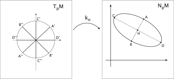
Figure 1. Ellipse of Curvature $\varepsilon_{\alpha}(\mathfrak{p})$ and Lines of Axial Curvature

As illustrated in Figure 1, to the small axis $AB$ is associated the crossing $A^{\prime}A^{\prime\prime}B^{\prime}B^{\prime\prime}$ and to the large axis $CD$ is associated the crossing $C^{\prime}C^{\prime\prime}D^{\prime}D^{\prime\prime}$. Thus, for each $\mathfrak{p}\in M$ at which the non-degenerate ellipse is not a circle or a point, two crossings are defined in $T_{\mathfrak{p}}M$, one associated to the large axis and the other to the small axis of the ellipse of curvature. These Fields of 2-Crossings in $M$ are called Fields of Axial Curvature.

Outside the set ${\mathcal{U}}_{\alpha}$ of points at which the ellipse of curvature is a circle (i.e. has equal axes), called Axiumbilic Points, the lines and crossings are said to be Lines and Crossings of Axial Curvature. Those related to the large (respectively small) axis of the ellipse of curvature are called Lines and Crossings of Principal (respectively Mean) Axial Curvature.

From the considerations above, the axial directions are defined by the equation

$$Jac(\|k_{n}-H\|^{2},I_{\alpha})=0$$

which has four solutions for $\mathfrak{p}\notin{\mathcal{U}}_{\alpha}$ and is singular at $\mathfrak{p}\in{\mathcal{U}}_{\alpha}$. According to [11] and [12], the differential equation of axial lines is given by:

(2) $$a_{4}dy^{4}+a_{3}dy^{3}dx+a_{2}dy^{2}dx^{2}+a_{1}dydx^{3}+a_{0}dx^{4}=0,$$

where

$$a_{4} = -4F(EG-2F^{2})(g_{1}^{2}+g_{2}^{2})+4G(EG-4F^{2})(f_{1}g_{1}+f_{2}g_{2}),$$

$$+ 8FG^{2}(f_{1}^{2}+f_{2}^{2})+4FG^{2}(e_{1}g_{1}+e_{2}g_{2})-4G^{3}(e_{1}f_{1}+e_{2}f_{2})$$

$$a_{3} = -4E(EG-4F^{2})(g_{1}^{2}+g_{2}^{2})-32EFG(f_{1}g_{1}+f_{2}g_{2}),$$

$$+ 16EG^{2}(f_{1}^{2}+f_{2}^{2})-4G^{3}(e_{1}^{2}+e_{2}^{2})+8EG^{2}(e_{1}g_{1}+e_{2}g_{2})$$

$$a_{2} = -12FG^{2}(e_{1}^{2}+e_{2}^{2})+12E^{2}F(EG-4F^{2})(g_{1}^{2}+g_{2}^{2}),$$

$$+ 24EG^{2}(e_{1}f_{1}+e_{2}f_{2})-24E^{2}G(f_{1}g_{1}+f_{2}g_{2})$$

$$a_{1} = 4E^{3}(g_{1}^{2}+g_{2}^{2})+4G(EG-4F^{2})(e_{1}^{2}+e_{2}^{2})$$

$$+ 32EFG(e_{1}f_{1}+e_{2}f_{2})-16E^{2}G(f_{1}^{2}+f_{2}^{2})-8E^{2}G(e_{1}g_{1}+e_{2}g_{2}),$$

$$a_{0} = 4F(EG-2F^{2})(e_{1}^{2}+e_{2}^{2})-4E(EG-4F^{2})(e_{1}f_{1}+e_{2}f_{2})$$

$$+ -8E^{2}F(f_{1}^{2}+f_{2}^{2})-4E^{2}F(e_{1}g_{1}+e_{2}g_{2})+4E^{3}(f_{1}g_{1}+f_{2}g_{2}).$$

Proposition 1 ([11], [12]).

Let $\alpha:M\longrightarrow\mathbb{R}^{4}$ be an immersion of class ${\mathcal{C}}^{r},\ r\geq 5$, of an oriented and smooth surface. Denote the first fundamental form of $\alpha$ by

$$I_{\alpha}=Edx^{2}+2Fdxdy+Gdy^{2}$$

and the second fundamental form by:

$$II_{\alpha}=(e_{1}dx^{2}+2f_{1}dxdy+g_{1}dy^{2})N_{1}+(e_{2}dx^{2}+2f_{2}dxdy+g_{2}dy^{2})N_{2}$$

where $\{N_{1},N_{2}\}$ is an orthonormal frame.

1. The differential equation of axial lines is given by:

   $${\mathcal{G}} = [a_{0}G(EG-4F^{2})+a_{1}F(2F^{2}-EG)]dy^{4}$$

   $$+ [-8a_{0}EFG+a_{1}E(4F^{2}-EG)]dy^{3}dx$$

   $$+ [-6a_{0}GE^{2}+3a_{1}FE^{2}]dy^{2}dx^{2}+a_{1}E^{3}dydx^{3}+a_{0}E^{3}dx^{4}=0,$$

   where

   $$a_{1} = 4G(EG-4F^{2})(e_{1}^{2}+e_{2}^{2})+32EFG(e_{1}f_{1}+e_{2}f_{2})$$

   $$+ 4E^{3}(g_{1}^{2}+g_{2}^{2})-8E^{2}G(e_{1}g_{1}+e_{2}g_{2})-16E^{2}G(f_{1}^{2}+f_{2}^{2})$$

   and

   $$a_{0} = 4F(EG-2F^{2})(e_{1}^{2}+e_{2}^{2})-4E(EG-4F^{2})(e_{1}f_{1}+e_{2}f_{2})$$

   $$+ 4E^{3}(f_{1}g_{1}+f_{2}g_{2})-4E^{2}F(e_{1}g_{1}+e_{2}g_{2})-8E^{2}F(f_{1}^{2}+f_{2}^{2}).$$

2. The axiumbilic points of $\alpha$ are characterized by $a_{0}=a_{1}=0$.

The axiumbilic points are defined by the intersection of the curves $a_{0}(x,y)=0$ and $a_{1}(x,y)=0$. Assume, with no lost of generality, that they intersect at $(x,y)=(0,0)$. In this work it will be considered the case where the intersection is transversal or quadratic at $(0,0)$.

Figure 2 illustrates the generic contact of the curves $a_{0}(x,y)=0$ and $a_{1}(x,y)=0$, whose intersection characterizes the axiumbilic points.

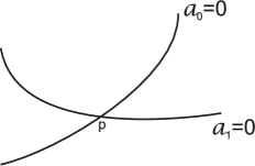
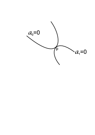
Figure 2. Transversal and quadratic contact between the curves $a_{0}=0$ and $a_{1}=0$ at an axiumbilic point $\mathfrak{p}$.

An axiumbilic point given by $(x,y)=(0,0)$ is called transversal if

(3) $$\frac{\partial(a_{0},a_{1})}{\partial(x,y)}\bigg{|}_{(0,0)}=\left|\begin{array}[]{cc}\frac{\partial a_{0}}{\partial x}(0,0)&\frac{\partial a_{0}}{\partial y}(0,0)\\ \frac{\partial a_{1}}{\partial x}(0,0)&\frac{\partial a_{1}}{\partial y}(0,0)\end{array}\right|\neq 0.$$

The axiumbilic point given by $(x,y)=(0,0)$ is said to be of quadratic type if the matrix

(4) $$\frac{\partial(a_{0},a_{1})}{\partial(x,y)}\bigg{|}_{(0,0)}=\left[\begin{array}[]{cc}\frac{\partial a_{0}}{\partial x}(0,0)&\frac{\partial a_{0}}{\partial y}(0,0)\\ \frac{\partial a_{1}}{\partial x}(0,0)&\frac{\partial a_{1}}{\partial y}(0,0)\end{array}\right]$$

has rank $1$ and, assuming $\frac{\partial a_{0}}{\partial y}(0,0)\neq 0$, it follows from the Implicit Function Theorem that $y(x)$ is a local solution of $a_{0}(x,y(x))=0$. Writing $s(x)=a_{1}(x,y(x))$ it follows that $s^{\prime}(0)=0$ and $s^{\prime\prime}(0)\neq 0$.

A similar analysis can be carried out if other element of the matrix $\frac{\partial(a_{0},a_{1})}{\partial(x,y)}\bigg{|}_{(0,0)}$ is non zero.

Remark 2 ([11]).

In isothermic coordinates, where $E=G$ and $F=0$, it follows that

$$a_{1}=-a_{3}=E^{3}[e_{1}^{2}+e_{2}^{2}+g_{1}^{2}+g_{2}^{2}-4(f_{1}^{2}+f_{2}^{2})-2(e_{1}g_{1}+e_{2}g_{2})]$$

$$a_{0}=a_{4}=-\frac{a_{2}}{6}=4E^{3}[f_{1}g_{1}+f_{2}g_{2}-(e_{1}f_{1}+e_{2}f_{2})]$$

and the differential equation of axial lines is simplified to

(5) $$a_{0}(x,y)(dx^{4}-6dx^{2}dy^{2}+dy^{4})+a_{1}(x,y)(dx^{2}-dy^{2})dxdy=0.$$

1.1. Axial Configurations of immersed surfaces in $\mathbb{R}^{4}$

Let ${\mathcal{I}}^{r}={\mathcal{I}}^{r}(M,\mathbb{R}^{4})$ the set of immersions of class ${\mathcal{C}}^{r}$. For $\alpha\in{\mathcal{I}}^{r}$, the differential equation of axial lines is well defined (equation (2)):

(6) $${\mathcal{G}}(x,y,dx,dy)=a_{4}dy^{4}+a_{3}dy^{3}dx+a_{2}dy^{2}dx^{2}+a_{1}dydx^{3}+a_{0}dx^{4}=0$$

in the projective bundle $PM$ of $M$.

For each $\alpha\in{\mathcal{I}}^{r}$, define the Lie-Cartan surface of the immersion $\alpha$ by ${\mathbb{L}}_{\alpha}:={\mathcal{G}}_{\alpha}^{-1}(0)$, which is of class ${\mathcal{C}}^{r-2}$, regular in $M-{\mathcal{U}}_{\alpha}$ and may present singularities at ${\mathcal{U}}_{\alpha}$. Moreover, as the differential equation (6) is quartic and contains the projective line at ${\mathcal{U}}_{\alpha}$, it follows that ${\mathbb{L}}_{\alpha}$ is a ramified covering of degree $4$ in $M-{\mathcal{U}}_{\alpha}$ and contains the projective line $\pi^{-1}(\mathfrak{p})$ for each $\mathfrak{p}\in{\mathcal{U}}_{\alpha}$.

In the chart $(x,y,p)$, with $p=\frac{dy}{dx}$, equation (6) is given by

(7) $${\mathcal{G}}(x,y,p)=a_{4}p^{4}+a_{3}p^{3}+a_{2}p^{2}+a_{1}p+a_{0}=0.$$

Consider the Lie-Cartan vector field $X_{\alpha}$, of class ${\mathcal{C}}^{r-3}$, tangent to the surface ${\mathcal{G}}=0$

(8) $$X_{\alpha}:={\mathcal{G}}_{p}\frac{\partial}{\partial x}+p{\mathcal{G}}_{p}\frac{\partial}{\partial y}-({\mathcal{G}}_{x}+p{\mathcal{G}}_{y})\frac{\partial}{\partial p}.$$

The axial curvature lines are the projections by $\pi:PM\longrightarrow M$ restricted to ${\mathbb{L}}_{\alpha}$, of the integral curves of $X_{\alpha}$.

See illustration in Figure 3. For each $\mathfrak{p}\in M-{\mathcal{U}}_{\alpha}$ there are $4$ well defined axial directions, given the four roots of equation (7).

Two axial configurations are given: Principal axial configuration ${\mathcal{P}}_{\alpha}=\{{\mathcal{U}}_{\alpha},{\mathcal{X}}_{\alpha}\}$ defined by the axiumbilic points ${\mathcal{U}}_{\alpha}$ and by the net ${\mathcal{X}}_{\alpha}$ (related to the crossing of principal axial curvature), in $M-{\mathcal{U}}_{\alpha}$ and Mean axial configuration ${\mathcal{Q}}_{\alpha}=\{{\mathcal{U}}_{\alpha},{\mathcal{Y}}_{\alpha}\}$ defined by the axiumbilic points ${\mathcal{U}}_{\alpha}$ and the net ${\mathcal{Y}}_{\alpha}$ (related to the crossing of mean axial curvature), in $M-{\mathcal{U}}_{\alpha}$.

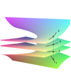
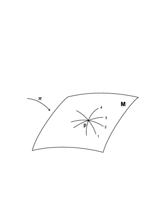
Figure 3. Projection on $M$ of the integral curves of the Lie-Cartan vector field tangent to ${\mathbb{L}}_{\alpha}$ in a neighborhood of $\mathfrak{p}\in M-{\mathcal{U}}_{\alpha}$. For each point in $M$ pass four lines, associated in pairs to the axis of the ellipse.

2. Differential Equation of Axial Lines in a Monge Chart

The surface $M$ will be locally parametrized by a Monge chart near an axiumbilic point $\mathfrak{p}$ as follows

$$\begin{array}[]{r}z=R(x,y),\\ w=S(x,y),\end{array}$$

where

(9) $$R(x,y)= \frac{r_{20}}{2}x^{2}+r_{11}xy+\frac{r_{02}}{2}y^{2}+\frac{r_{30}}{6}x^{3}+\frac{r_{21}}{2}x^{2}y+\frac{r_{12}}{2}xy^{2}+\frac{r_{03}}{6}y^{3}$$

$$+ \frac{r_{40}}{24}x^{4}+\frac{r_{31}}{6}x^{3}y+\frac{r_{22}}{4}x^{2}y^{2}+\frac{r_{13}}{6}xy^{3}+\frac{r_{04}}{24}y^{4}+h.o.t.,$$

(10) $$S(x,y)= \frac{s_{20}}{2}x^{2}+s_{11}xy+\frac{s_{02}}{2}y^{2}+\frac{s_{30}}{6}x^{3}+\frac{s_{21}}{2}x^{2}y+\frac{s_{12}}{2}xy^{2}+\frac{s_{03}}{6}y^{3}$$

$$+ \frac{s_{40}}{24}x^{4}+\frac{s_{31}}{6}x^{3}y+\frac{s_{22}}{4}x^{2}y^{2}+\frac{s_{13}}{6}xy^{3}+\frac{s_{04}}{24}y^{4}+h.o.t.$$

At the point $(x,y,R(x,y),S(x,y))$, the tangent plane to the surface is generated by $\{t_{1},t_{2}\}$, where $t_{1}=(1,0,R_{x},S_{x})$ and $t_{2}=(0,1,R_{y},S_{y})$. The normal plane is generated by $\{N_{1},N_{2}\}$, where $N_{1}=\frac{\widetilde{N_{1}}}{|\widetilde{N_{1}}|}$ and $N_{2}=\frac{\widetilde{N_{2}}}{|\widetilde{N_{2}}|}$ are defined by $\widetilde{N_{1}}=(-R_{x},-R_{y},1,0)$ and $\widetilde{N_{2}}=t_{1}\wedge t_{2}\wedge\widetilde{N_{1}}$. Here $\wedge$ is the exterior or wedge product of three vectors in $\mathbb{R}^{4}$, defined by the equation:

$$\det(t_{1},t_{2},\widetilde{N_{1}},\bullet)=\langle\widetilde{N_{2}},\bullet\rangle.$$

From the expressions of $R$ and $S$ given by equations (9) and (10), it follows that:

$$E=1+O(2),\hskip 28.45274pt\ F=O(2),\hskip 28.45274pt\ G=1+O(2),$$

and

$$\begin{array}[]{cc}e_{1}=r_{20}+r_{30}x+r_{21}y+O(2),&e_{2}=s_{20}+s_{30}x+s_{21}y+O(2),\\ f_{1}=r_{11}+r_{21}x+r_{12}y+O(2),&f_{2}=s_{11}+s_{21}x+s_{12}y+O(2),\\ g_{1}=r_{02}+r_{12}x+r_{03}y+O(2),&g_{2}=s_{02}+s_{12}x+s_{03}y+O(2).\end{array}$$

The axiumbilic points are defined by $a_{0}(x,y)=0$ and $a_{1}(x,y)=0$. So, in a neighborhood of $(0,0)$, it follows that

(11) $$a_{0}(x,y)=a^{0}_{00}+a^{0}_{10}x+a^{0}_{01}y+O(2)$$

and

(12) $$a_{1}(x,y)=a^{1}_{00}+a^{1}_{10}x+a^{1}_{01}y+O(2),$$

where

$$a^{0}_{00} = r_{11}(r_{02}-r_{20})+s_{11}(s_{02}-s_{20}),$$

$$a^{0}_{10} = r_{21}(r_{02}-r_{20})+r_{11}(r_{12}-r_{30})+s_{11}(s_{12}-s_{30})+s_{21}(s_{02}-s_{20}),$$

$$a^{0}_{01} = r_{12}(r_{02}-r_{20})+r_{11}(r_{03}-r_{21})+s_{11}(s_{03}-s_{21})+s_{12}(s_{02}-s_{20})$$

and

$$a^{1}_{00} = (r_{02}-r_{20})^{2}+(s_{02}-s_{20})^{2}-4(r_{11}^{2}+s_{11}^{2}),$$

$$a^{1}_{10} = 2(r_{12}-r_{30})(r_{02}-r_{20})+2(s_{12}-s_{30})(s_{02}-s_{20})-8(r_{21}r_{11}+s_{21}s_{11}),$$

$$a^{1}_{01} = 2(r_{03}-r_{21})(r_{02}-r_{20})+2(s_{03}-s_{21})(s_{02}-s_{20})-8(r_{12}r_{11}+s_{12}s_{11}).$$

Therefore a point $\mathfrak{p}$, expressed in a Monge chart by $(0,0)$, is an axiumbilic point when the following relations hold.

(13) $$\left\{\begin{array}[]{l}a^{0}_{00}=r_{11}(r_{02}-r_{20})+s_{11}(s_{02}-s_{20})=0,\\ a^{1}_{00}=(r_{02}-r_{20})^{2}+(s_{02}-s_{20})^{2}-4(r_{11}^{2}+s_{11}^{2})=0.\end{array}\right.$$

Algebraic manipulations of the equations above, see [2], show that $(0,0)$ is an axiumbilic point when the following equations hold

(14) $$\left\{\begin{array}[]{lcl}2r_{11}=(s_{02}-s_{20}),\\ 2s_{11}=-(r_{02}-r_{20},)\end{array}\right.\hskip 56.9055pt\mbox{or}\hskip 56.9055pt\left\{\begin{array}[]{lcl}2r_{11}=-(s_{02}-s_{20}),\\ 2s_{11}=(r_{02}-r_{20}).\end{array}\right.$$

Remark 3.

Let $r_{02}=r_{20}+r$ and $s_{02}=s_{20}+s$, $\rho^{2}=r^{2}_{11}+s^{2}_{11}$. Then the condition for $(0,0)$ to be an axiumbilic point, see equation (13), is given by

(15) $$\left\{\begin{array}[]{l}r_{11}\cdot r+s_{11}\cdot s=0,\\ r^{2}+s^{2}=4\rho^{2}.\end{array}\right.$$

These condition for being an axiumbilic point can be interpreted as the intersection of a circle and a straight line in the plane $(r,s)$. The intersections are given by

(16) $$\left\{\begin{array}[]{lcl}r_{11}=\frac{s}{2},\\ s_{11}=-\frac{r}{2},\end{array}\right.\hskip 56.9055pt\mbox{or}\hskip 56.9055pt\left\{\begin{array}[]{lcl}r_{11}=-\frac{s}{2},\\ s_{11}=\frac{r}{2},\end{array}\right.$$

and therefore equation (16) is another form of equation (14).

Let

$$\alpha_{1}= s_{12}-s_{30}+2r_{21},\;\alpha_{2}=r_{30}-r_{12}+2s_{21},$$

$$alpha_{3}= s_{03}-s_{21}+2r_{12},\;\alpha_{4}=r_{21}-r_{03}+2s_{12}.$$

The discussion above is synthesized in the following lemma.

Lemma 4.

Let $\mathfrak{p}$ be an axiumbilic point with coordinates $(0,0)$ in a Monge chart. The differential equation of axial lines in a neighborhood of $(0,0)$ is given by

(17) $$\tilde{a}_{0}(x,y)(dx^{4}-6dx^{2}dy^{2}+dy^{4})+\tilde{a}_{1}(x,y)(dx^{2}-dy^{2})dxdy+H(x,y,dx,dy)=0,$$

where

(18) $$\tilde{a}_{0}(x,y)= \frac{1}{2}(r\alpha_{1}+s\alpha_{2})x+\frac{1}{2}(r\alpha_{3}+s\alpha_{4})y+a^{0}_{20}x^{2}+a^{0}_{11}xy+a^{0}_{02}y^{2},$$

$$\tilde{a}_{1}(x,y)= 2(s\alpha_{1}-r\alpha_{2})x+2(s\alpha_{3}-r\alpha_{4})y+a^{1}_{20}x^{2}+a^{1}_{11}xy+a^{1}_{02}y^{2}$$

and $H$ contains terms of order greater than or equal to $3$ in $(x,y)$.

With the notation in equation (17), the condition of transversality between the curves $a_{0}=0$ and $a_{1}=0$ is given by

$$\left|\begin{array}[]{cc}a^{0}_{10}&a^{0}_{01}\\ a^{1}_{10}&a^{1}_{01}\end{array}\right|\neq 0.$$

The determinant above has the following expression:

$$[\alpha_{2}\alpha_{3}-\alpha_{1}\alpha_{4}]\cdot(r^{2}+s^{2}),$$

where $r=r_{02}-r_{20}$ and $s=s_{02}-s_{20}$. If $(r^{2}+s^{2})$ is zero, it follows that $a^{0}_{10}=a^{0}_{01}=a^{1}_{10}=a^{1}_{01}=0$, and therefore the matrix

$$\left[\begin{array}[]{cc}a^{0}_{10}&a^{0}_{01}\\ a^{1}_{10}&a^{1}_{01}\end{array}\right]$$

is identically zero. Thus the axiumbilic points with $r=s=0$ form a set of codimension at least four.

Therefore, the condition of transversality, supposing $r^{2}+s^{2}\neq 0$, is given by:

(19) $$T:=\alpha_{2}\alpha_{3}-\alpha_{1}\alpha_{4}\neq 0.$$

Long, but straightforward calculations show that the condition (19) is invariant by positive rotations in the tangent and in the normal plane.

Lemma 5.

Consider the quartic differential equation

$$(a_{10}x+a_{01}y)(dx^{4}-6dx^{2}dy^{2}+dy^{4})+(b_{10}x+b_{01}y)dxdy(dx^{2}-dy^{2})=0.$$

Consider a rotation $x=\cos\theta u+\sin\theta v,\;y=-\sin\theta u+\cos\theta v$, where $\theta$ is a real root of the equation

$$-a_{01}t^{5}+(a_{10}-b_{01})t^{4}+(6a_{01}+b_{10})t^{3}+(b_{01}-6a_{10})t^{2}-(a_{01}+b_{10})t+a_{10}=0,\;t=\tan\theta.$$

Then it follows that

$$\bar{a_{01}}v(du^{4}-6du^{2}dv^{2}+dv^{4})+(\bar{b_{10}}u+\bar{b_{01}}v)dudv(du^{2}-dv^{2})=0.$$

where $\bar{a_{01}}=\bar{a_{01}}(a_{10},a_{01},b_{10},b_{01},\theta)$, $\bar{b_{10}}=\bar{b_{10}}(a_{10},a_{01},b_{10},b_{01},\theta)$ and $\bar{b_{01}}=\bar{b_{01}}(a_{10},a_{01},b_{10},b_{01},\theta)$.

Proof.

The result follows from straightforward calculations. Observe that when $a_{01}=0$ a rotation of angle $\pi/2$ is sufficient to obtain the result stated. ∎

Proposition 6.

Let $\mathfrak{p}$ be an axiumbilic point. Then there exists a Monge chart and a homotety in $\mathbb{R}^{4}$ such that the differential equation of axial lines is given by

(20) $$y(dy^{4}-6dx^{2}dy^{2}+dx^{4})+(ax+by)dxdy(dx^{2}-dy^{2})+H(x,y,dx,dy)=0$$

where $H$ contains terms of order greater than or equal to $2$ in $(x,y)$. Moreover, the axiumbilic point $\mathfrak{p}$ is transversal if and only if $a\neq 0$.

Proof.

Consider a parametrization $X(x,y)=(x,y,R(x,y),S(x,y))$ given by equations (9) and (10) such that $0$ is an axiumbilic point. By equation (18) it follows that:

$$a_{0}(x,y)= \frac{1}{2}(r\alpha_{1}+s\alpha_{2})x+\frac{1}{2}(r\alpha_{3}+s\alpha_{4})y+O(2),$$

$$a_{1}(x,y)= 2(s\alpha_{1}-r\alpha_{2})x+2(s\alpha_{3}-r\alpha_{4})y+O(2).$$

By an appropriate choice of the rotation in the plane $\{x,y\}$ given by Lemma 5 and a homotety in $\mathbb{R}^{4}$, it is possible to make $2a_{10}=r\alpha_{1}+s\alpha_{2}=0$ and, when $(\alpha_{1}\alpha_{4}-\alpha_{2}\alpha_{3})(r^{2}+s^{2})\neq 0$, also $a_{01}=\frac{1}{2}(r\alpha_{3}+s\alpha_{4})=1$. So the result is established, $a=\frac{4(s\alpha_{1}-r\alpha_{2})}{r\alpha_{3}+s\alpha_{4}}$ when $r\alpha_{1}+s\alpha_{2}=0$ and $b=\frac{4(s\alpha_{3}-r\alpha_{4})}{r\alpha_{3}+s\alpha_{4}}$. If $r\neq 0$ it follows that $a=-\frac{4(r^{2}+s^{2})\alpha_{2}}{r(r\alpha_{3}+s\alpha_{4})}$ and $a=\frac{4\alpha_{1}}{\alpha_{4}}$ when $s\neq 0$ and $r=0$. ∎

Remark 7.

Let $p=\frac{dy}{dx}$. Then the differential equation (20) is given by:

(21) $$y(p^{4}-6p^{2}+1)+(ax+by)p(1-p^{2})+H(x,y,p)=0,$$

where $H$ contains terms of order greater than or or equal to $2$ in $(x,y)$.

3. Axial configuration in the neighborhood of axiumbilic points

Let $\mathfrak{p}$ be an axiumbilic point whose neighborhood is parametrized by a Monge chart following the notation established in Section 2. When it is a transversal axiumbilic point, which is determined by transversal intersection of the curves $a_{0}=0$ and $a_{1}=0$ (see equation (3)), it results from Proposition 6 and Remark 7 that the differential equation of axial lines is given by

(22) $${\mathcal{G}}(x,y,p)=y(p^{4}-6p^{2}+1)+(ax+by)p(1-p^{2})+H(x,y,p)=0,$$

where $H(x,y,p)$ contains higher order terms greater or equal to $2$ in $(x,y)$.

The Lie-Cartan surface $\mathbb{L}_{\alpha}$ in $PM$ is defined implicitly by

(23) $${\mathcal{G}}(x,y,p)=0.$$

In the case that $\mathfrak{p}$ is a transversal axiumbilic point the surface defined above is regular and of class ${\mathcal{C}}^{r-2}$ in the neighborhood of the projective axis $p$.

In the coordinates $(x,y,p)$, the Lie-Cartan vector field $X$, is of class ${\mathcal{C}}^{r-3}$, (equation (8)):

(24) $$X:={\mathcal{G}}_{p}\frac{\partial}{\partial x}+p{\mathcal{G}}_{p}\frac{\partial}{\partial y}-({\mathcal{G}}_{x}+p{\mathcal{G}}_{y})\frac{\partial}{\partial p}$$

and the projections of the integral curves of $X\bigg{|}_{{\mathcal{G}}=0}$ are the axial lines in a neighborhood of $\mathfrak{p}$ (Figure 3).

Restricted to the projective axis $p$ the Lie-Cartan vector field is given by

$$X=-p[(p^{4}-6p^{2}+1)+(1-p^{2})(a+bp)]\frac{\partial}{\partial p}.$$

Therefore, the singular points of the Lie-Cartan vector field in the projective line are given by the equation:

(25) $$P(p)=pR(p)=p[(p^{4}-6p^{2}+1)+(1-p^{2})(a+bp)]=0.$$

The discriminant of $R(p)=(p^{4}-6p^{2}+1)+(1-p^{2})(a+bp)$ is

(26) $$\Delta(a,b)= 16a^{5}+4(b^{2}+68)a^{4}+16(b^{2}+144)a^{3}$$

$$- 8(b^{2}-80)(16+b^{2})a^{2}+96(16+b^{2})^{2}a+4(16+b^{2})^{3}.$$

Furthermore, $R(\pm 1)=-4$, $R(0)=1+a$ and $\lim_{p\longrightarrow\pm\infty}R(p)=+\infty$, thus $R$ has at least two simple real roots, one is less than $-1$ and the other is greater than $1$.

The derivative of $X$ at $(0,0,p)$ is given by:

$$DX(0,0,p)=\left[\begin{array}[]{ccc}a(1-3p^{2})&4p^{3}+b(1-3p^{2})-12p&0\\ a(1-3p^{2})p&p[4p^{3}+b(1-3p^{2})-12p]&0\\ 0&0&-P^{\prime}(p)\end{array}\right]$$

whose eigenvalues are $0$ and

$$\begin{array}[]{l}\lambda_{1}(p)=a(1-3p^{2})+p[4p^{3}+b(1-3p^{2})-12p],\\ \lambda_{2}(p)=-P^{\prime}(p).\\ \end{array}$$

Recall that $P(p)=pR(p)$, and so $P^{\prime}(p)=R(p)+pR^{\prime}(p)$. Therefore at the roots of $R$, it follows that $-P^{\prime}(p)=-pR^{\prime}(p)$. Also, as $\pm 1$ are not roots of $R$, it follows that

$$a=\frac{(-p^{4}+6p^{2}-1)+bp(1-p^{2})}{1-p^{2}}.$$

Substituting the equation above into the expression of $\lambda_{1}(p)$, $p$ being a root of $R(p)$ (singular points of $X$), it follows that

$$\left\{\begin{array}[]{l}\lambda_{1}(p)=\frac{(p^{2}+1)^{3}}{(p^{2}-1)},\\ \lambda_{2}(p)=-pR^{\prime}(p).\\ \end{array}\right.$$

Therefore, the eigenvalues of $DX$, on the tangent space to $\mathcal{G}=0$, are as follows:

(27) $$p_{0}=0:\ \ \left\{\begin{array}[]{l}\lambda_{1}=a,\\ \lambda_{2}=-(a+1),\end{array}\ \ \ \ \right.$$

(28) $$p_{i}\neq 0:\ \ \left\{\begin{array}[]{l}\lambda_{1}=\frac{(p_{i}^{2}+1)^{3}}{(p_{i}^{2}-1)},\\ \lambda_{2}=-p_{i}R^{\prime}(p_{i}).\\ \end{array}\ \ \ \ \right.$$

The eigenspace associated to the eigenvalue $\lambda_{1}$ is transversal to the axis $p$ and the eigenvalue $\lambda_{2}$ has the projective axis as the associated eigenspace.

In [11] the axial configuration near an axiumbilic point was established in the following situation:

• $\Delta(a,b)<0$,

• $\Delta(a,b)>0$,  $a<0,\;a\neq-1$,

• $\Delta(a,b)>0$,  $a>0$.

When $\Delta(a,b)<0$, $R$ has two simple real roots, and the Lie-Cartan vector field has three hyperbolic saddles in the projective axis. This axiumbilic point is called of type $E_{3}$.

When $\Delta(a,b)>0$, $a<0,\ a\neq-1$, $R$ has four simple real roots, and the Lie-Cartan vector field has 5 singular points in the projective line. Four are hyperbolic saddles and one is a hyperbolic node. This axiumbilic point is called of type $E_{4}$.

When $\Delta(a,b)>0$, $a>0$, the Lie-Cartan vector field has 5 hyperbolic saddles in the projective line. This axiumbilic point is called of type $E_{5}$.

In Figure 4 the Lie-Cartan surfaces and the integral curves of the Lie-Cartan vector field are sketched in the three cases $E_{3}$, $E_{4}$ and $E_{5}$. The projections of the integral curves by $\pi:PM\longrightarrow M$ are the axial lines near the axiumbilic points (see Figure 5) $E_{3}$, $E_{4}$ and $E_{5}$.

         

Figure 4. Lie-Cartan vector field and its integral curves in the cases $E_{3}$, $E_{4}$ and $E_{5}$.

                

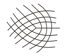
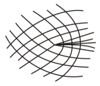
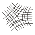
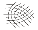
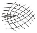
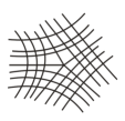
Figure 5. Axial Configurations near Axiumbilic Points $E_{3}$ (left), $E_{4}$ (center) and $E_{5}$ (right).

For an immersion $\alpha$ of a surface $M$ into $\mathbb{R}^{4}$, the axiumbilic singularities ${\mathcal{U}}_{\alpha}$ and the lines of axial curvature are assembled into two axial configurations: the principal axial configuration ${\mathcal{P}}_{\alpha}=\{{\mathcal{U}}_{\alpha},\;{\mathcal{X}}_{\alpha}\}$ and the mean axial configuration ${\mathcal{Q}}_{\alpha}=\{{\mathcal{U}}_{\alpha},\;{\mathcal{Y}}_{\alpha}\}.$

An immersion $\alpha\in{\mathcal{I}}^{r}$ is said to be Principal Axial Stable if it has a $C^{r}$ neighborhood ${\mathcal{V}}(\alpha)$ such that, for any $\beta\in{\mathcal{V}}(\alpha)$ there exists a homeomorphism $h:M\to M$ mapping ${\mathcal{U}}_{\alpha}$ onto ${\mathcal{U}}_{\beta}$ and mapping the integral net of ${\mathcal{X}}_{\alpha}$ onto that of ${\mathcal{X}}_{\beta}$. Analogous definition is given for Mean Axial Stability.

In Proposition 8 are described the axiumbilic points which are axial stable. In Figure 6 are sketched the curves $\Delta(a,b)=0$, $a=-1$ and $a=0$ in the plane $a,b$, which bound the open regions corresponding to the three types of axiumbilic points of axial stable type.

Proposition 8 ([11], [12] p. 209).

Let $\mathfrak{p}$ be an axiumbilic point of $\alpha\in{\mathcal{I}}^{r},\ r\geq 5$. Then, $\alpha$ is locally principal axial stable and locally mean axial stable at $\mathfrak{p}$ if and only if $\mathfrak{p}$ is of type $E_{3},\ E_{4}$ or $E_{5}$. The curve $\Delta(a,b)=0$ has three connected components, is contained in the region $a\leq-1$ and it is regular outside the points $(-\frac{27}{2},\pm\frac{5\sqrt{5}}{2})$ which are of cuspidal type.

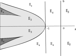
Figure 6. Diagram of stable axiumbilic points, $E_{3}$, $E_{4}$ and $E_{5}$.

Proof.

The function $\Delta(a,b)$ defined by equation (26) is symmetric in $b$. The polynomials $\Delta(a,b)$ and $\frac{\partial\Delta}{\partial b}$ in the variable $b$ has resultant equal to $274877906944(1+a)(a^{2}+8a+32)^{2}a^{16}(2a+27)^{6}$.

The critical points $p_{\pm}=(-\frac{27}{2},\pm\frac{5\sqrt{5}}{2})$ of $\Delta$ are contained in $\Delta(a,b)=0$.

Near the point $p_{+}$ it follows that:

$$\Delta(a,b)= -54675\left[\left(a+\frac{27}{2}\right)^{2}+5\left(b-\frac{5\sqrt{5}}{2}\right)^{2}+2\sqrt{5}\left(a+\frac{27}{2}\right)\left(b-\frac{5\sqrt{5}}{2}\right)\right]$$

$$+ h.o.t.$$

Further analysis shows $p_{\pm}$ are Whitney cuspidal points.

Also the curve $\Delta(a,b)=0$ is contained in the region $a\leq-1$ and near $(-1,0)$ it is given by $a=-\frac{1}{20}b^{2}+O(3)$. In fact, for $a>-1$ all the roots of $\Delta(a,b)$ are complex.

By the classification of axiumbilic points $E_{3}$, $E_{4}$ and $E_{5}$ by the sign of $\Delta(a,b)$ and of $a$, the diagram of stable axiumbilic points, see [11], [12] p. 209, is as shown in Fig. 6. ∎

3.1. The axiumbilic point $E^{1}_{34}$

Definition 9.

Let $\alpha:M\longrightarrow\mathbb{R}^{4}$ be an immersion of class ${\mathcal{C}}^{r},r\geq 5,$ of a smooth and oriented surface. An axiumbilic point $\mathfrak{p}$ is said to be of type $E^{1}_{34}$ if $a$ defined in Proposition 6 does not vanish and:

1. $\Delta(a,b)=0$, $(a,b)\neq(-1,0)$ and $(a,b)\neq(-\frac{27}{2},\pm\frac{5}{2}\sqrt{5})$, or

2. $b\neq 0$ if $a=-1.$

Proposition 10.

Let $\alpha:M\longrightarrow\mathbb{R}^{4}$ be an immersion of class ${\mathcal{C}}^{r},\ r\geq 5$ of a smooth and oriented surface having an axiumbilic point $\mathfrak{p}$ of type $E^{1}_{34}$. Then the axial configuration of $\alpha$ in a neighborhood of $\mathfrak{p}$ is as shown in Figure 7.

               

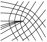
Figure 7. Axial Configurations in a neighborhood of an axiumbilic point of type $E^{1}_{34}$.

Proof.

Since the condition of transversality ($a\neq 0$) is preserved at an axiumbilic point of type $E^{1}_{34}$ the implicit surface defined by equation (23) is regular in a neighborhood of the projective line. From the hypotheses $\Delta(a,b)=0$, $(a,b)\neq(-1,0)$ and $(a,b)\neq(-\frac{27}{2},\pm\frac{5}{2}\sqrt{5})$ or $b\neq 0$, if $a=-1$, the polynomial $P(p)=p[(p^{4}-6p^{2}+1)+(1-p^{2})(a+bp)]=pR(p)$, which defines the singularities of the Lie-Cartan vector field, has one double root and three real simple roots.

With no loss of generality, we can consider the case $a=-1$ and $b\neq 0$, where $p=0$ is a double root of the polynomial $P(p)$. In this case, we have $P(p)=p^{2}(p^{3}-bp^{2}-5p+b)$.

The eigenvalues of $DX$ at $(0,0,p)$ are given by: $\lambda_{1}=4p^{4}-3bp^{3}-9p^{2}+bp-1$ and $\lambda_{2}=p(-5p^{3}+4bp^{2}+15p-2b)$.

Therefore, at the singular points $(0,0,p)$, $p\neq 0$, of $X$ it follows that: $\lambda_{1}=\frac{(p^{2}+1)^{3}}{p^{2}-1}$ and $\lambda_{2}=-\frac{p^{2}(p^{4}+2p^{2}+5)}{p^{2}-1}$. Then, $\lambda_{1}\lambda_{2}<0$ when $p\neq 0$ and these three singular points of $X$ are hyperbolic saddles. At $p=0$, double root of $P$, it follows that $\lambda_{1}=-1,\;\lambda_{2}=0$. Recall that the eigenspace associated to $\lambda_{1}$ is transversal to the axis $p$ and that one associated to $\lambda_{2}$ is the projective axis itself.

Since ${\mathcal{G}}_{y}(0,0,0)=1$, it follows from the Implicit Function Theorem that $y(x,p)=xp+O(3)$ is defined in a neighborhood of $(0,0,0)$ such that ${\mathcal{G}}(x,y(x,p),p)=0$. In this case, the Lie-Cartan vector field in the chart $(x,p)$ is given by:

(29) $$\left\{\begin{array}[]{l}\dot{x}=-x+bxp+O(3)\\ \dot{p}=-bp^{2}+O(3)\end{array}\right.$$

with $b\neq 0$. Therefore, $(0,0,0)$ is a quadratic saddle-node with the center manifold tangent to the projective line. The phase portrait is sketched in Figure 8, and the projections of the integral curves are the axial lines shown in Figure 7.

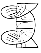
Figure 8. Integral curves of $X|_{{\mathcal{G}}=0}$ in the neighborhood of the projective line in the case of an axiumbilic point of type $E^{1}_{34}$

When $(a,b)\neq(-1,0)$, $(a,b)\neq(-\frac{27}{2},\pm\frac{5}{2}\sqrt{5})$ and $\Delta(a,b)=0$ the polynomial $P(p)=p[(p^{4}-6p^{2}+1)+(1-p^{2})(a+bp)]$ has a double root $p_{0}\neq 0$ and three real simple roots. This case is reduced to the case when $p=0$ is a double root, making an appropriated rotation of coordinates in the plane $\{x,y\}$ so that the double root $p_{0}$ is, in the new coordinates, located at $p=0$. ∎

Proposition 11.

Let $\alpha\in{\mathcal{I}}^{r}$, $r\geq 5$, be an immersion such that $\mathfrak{p}$ is axiumbilic point of type $E^{1}_{34}$. Then, there is a neighborhood $V$ of $\mathfrak{p}$, a neighborhood ${\mathcal{V}}$ of $\alpha$ and a function ${\mathcal{F}}:{\mathcal{V}}\longrightarrow\mathbb{R}$ of class ${\mathcal{C}}^{r-3}$ such that for each $\mu\in{\mathcal{V}}$ there is an unique axiumbilic point $\mathfrak{p}_{\mu}\in V$ such that:

1. $d{\mathcal{F}}_{\alpha}\neq 0$,

2. ${\mathcal{F}}(\mu)<0$ if and only if $\mathfrak{p}_{\mu}$ is axiumbilic point of type $E_{3}$,

3. ${\mathcal{F}}(\mu)>0$ if and only if $\mathfrak{p}_{\mu}$ is axiumbilic point of type $E_{4}$,

4. ${\mathcal{F}}(\mu)=0$ if, and only if, $\mathfrak{p}_{\mu}$ is axiumbilic point of type $E^{1}_{34}$.

Proof.

Since $\mathfrak{p}$ is a transversal axiumbilic point of $\alpha$, the existence of the neighborhoods ${\mathcal{V}}$ and $V$ follows from the Implicit Function Theorem. For $\mu\in{\mathcal{V}}$ with an axiumbilic point $\mathfrak{p}_{\mu}\in V$, after a rigid motion $\Gamma_{\mu}$ in $\mathbb{R}^{4}$, locally the immersion $\mu\in{\mathcal{V}}$ can be parametrized in terms of a Monge chart $(x,y,R_{\mu}(x,y),S_{\mu}(x,y))$, with the origin being the axiumbilic point $p_{\mu}$ and

$$R_{\mu}(x,y)= \frac{r_{20}(\mu)}{2}x^{2}+r_{11}(\mu)xy+\frac{r_{02}(\mu)}{2}y^{2}+\frac{r_{30}(\mu)}{6}x^{3}+\frac{r_{31}(\mu)}{2}x^{2}y$$

$$+ \frac{r_{13}(\mu)}{2}xy^{2}+\frac{r_{03}(\mu)}{6}y^{3}+h.o.t.,$$

$$S_{\mu}(x,y)= \frac{s_{20}(\mu)}{2}x^{2}+s_{11}(\mu)xy+\frac{s_{02}(\mu)}{2}y^{2}+\frac{s_{03}(\mu)}{6}x^{3}+\frac{s_{21}(\mu)}{2}x^{2}y$$

$$+ \frac{s_{12}(\mu)}{2}xy^{2}+\frac{s_{03}(\mu)}{6}y^{3}+h.o.t.$$

For $\mu$, performing rotations and homoteties as described in Section 2, the coefficients $a_{\mu}$ and $b_{\mu}$ can be expressed in function of the coefficients of the surface presented in a Monge chart, as was done in Proposition 6, considering the coefficients in function of the parameter $\mu\in{\mathcal{V}}$.

Define ${\mathcal{F}}(\mu)=\Delta(a(\mu),b(\mu))$ whose zeros define locally the manifold of immersions with an $E_{34}^{1}$ axiumbilic point. Here, $\Delta(a,b)$, given by equation (26), is the discriminant of the polynomial $R(p)=(p^{4}-6p^{2}+1)+(1-p^{2})(a+bp)$.

Notice that due to the particular representation of the 3-jets taken here, the condition $a(\mu)=-1$ in Definition 9, the jet extension of the immersion is not transversal, but tangent, to the manifold of jets with $E_{34}^{1}$ axiumbilic points. It is always possible, by an appropriate rotation in the plane $\{x,y\}$ to suppose that $a(\alpha)\notin\{-\frac{27}{2},-1\}$. See Section 2.

Assertions $(ii),(iii)$ and $(iv)$ follow from the definition of ${\mathcal{F}}$ and the previous analysis on the sign of the discriminant $\Delta(a_{\mu},b_{\mu})$.

Moreover, the derivative of ${\mathcal{F}}(\mu)$ in the direction of the coordinate $a$ does not vanish, leading to conclude that $d{\mathcal{F}}_{\alpha}\neq 0$.

In fact, assuming $s_{11}(\alpha)=\frac{1}{2}r\neq 0$, it follows that

$$a_{0}(\mu)= y+0(2),$$

$$a_{1}(\mu)(x,y)= -\frac{4(r(\mu)^{2}+s(\mu)^{2})\alpha_{2}(\mu)}{r(\mu)\left(r(\mu)\alpha_{3}(\mu)+s(\mu)\alpha_{4}(\mu)\right)}x$$

$$+ \frac{4(s(\mu)\alpha_{3}(\mu)-r(\mu)\alpha_{4}(\mu))}{r(\mu)\alpha_{3}(\mu)+s(\mu)\alpha_{4}(\mu)}y+O(2)$$

$$= a(\mu)x+b(\mu)y+O(2),$$

$$\alpha_{1}= s_{12}-s_{30}+2r_{21},\;\alpha_{2}=r_{30}-r_{12}+2s_{21},$$

$$\;\alpha_{3}= s_{03}-s_{21}+2r_{12},\;\alpha_{4}=r_{21}-r_{03}+2s_{12}$$

Consider the deformation

$$\mu=\left(x,y,R_{\alpha}(x,y),S_{\alpha}(x,y)\right)+\left(0,0,t(\frac{1}{6}x^{3}-\frac{1}{2}xy^{2}),tx^{2}y\right).$$

Then, as $\alpha_{2}=r_{30}-r_{12}+2s_{21}$, it follows that $a(\mu)=-\frac{4(r^{2}+s^{2})(\alpha_{2}+t)}{r\left(r\alpha_{3}+s\alpha_{4}\right)}$ and

$$\frac{d}{dt}\left(\Delta(a(\mu),b(\mu)\right)\bigg{|}_{t=0}=\frac{\partial\Delta}{\partial a}\cdot\frac{da}{dt}=\frac{\partial\Delta}{\partial a}\cdot\left(-\frac{4(r^{2}+s^{2})}{r(r\alpha_{3}+s\alpha_{4})}\right)\neq 0.$$

In the case where $s_{11}(\alpha)=0$ it follows that $r_{11}(\alpha)=-\frac{1}{2}s\neq 0$, $\alpha_{1}\alpha_{4}\neq 0$ and $\alpha_{2}(\mu)=0$. Now consider the deformation

$$\mu=\left(x,y,R_{\alpha}(x,y),S_{\alpha}(x,y)\right)+\left(0,0,tx^{2}y,t(-\frac{1}{6}x^{3}+\frac{1}{2}xy^{2})\right).$$

Then, $a(\mu)=\frac{4(\alpha_{1}+t)}{\alpha_{4}}$ and

$$\frac{d}{dt}\left(\Delta(a(\mu),b(\mu)\right)\bigg{|}_{t=0}=\frac{\partial\Delta}{\partial a}\cdot\frac{da}{dt}=\frac{\partial\Delta}{\partial a}\cdot\left(\frac{4}{\alpha_{4}}\right)\neq 0.$$

∎

                                                        

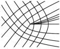
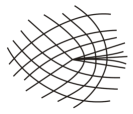
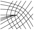
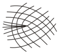
Figure 9. Axial configuration near axiumbilic points. $E_{3}$ (left), $E^{1}_{34}$ (center) and $E_{4}$ (right).

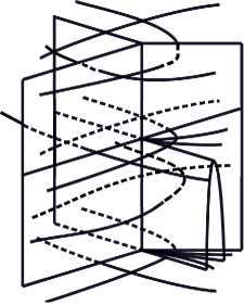
Figure 10. Bifurcation diagram of the axial configuration near an axiumbilic point $E^{1}_{34}$ and the structure of separatrices.

3.2. The axiumbilic point $E^{1}_{4,5}$

Consider the Monge chart described by equations (9) and (10). Suppose that the origin is an axiumbilic point, which is expressed by

(30) $$R(x,y)= \frac{r_{20}}{2}x^{2}+r_{11}xy+\frac{r_{02}}{2}y^{2}+\frac{r_{30}}{6}x^{3}+\frac{r_{21}}{2}x^{2}y+\frac{r_{12}}{2}xy^{2}+\frac{r_{03}}{6}y^{3}$$

$$+ \frac{r_{40}}{24}x^{4}+\frac{r_{31}}{6}x^{3}y+\frac{r_{22}}{4}x^{2}y^{2}+\frac{r_{13}}{6}xy^{3}+\frac{r_{04}}{24}y^{4}+h.o.t.,$$

(31) $$S(x,y)= \frac{s_{20}}{2}x^{2}+s_{11}xy+\frac{s_{02}}{2}y^{2}+\frac{s_{30}}{6}x^{3}+\frac{s_{21}}{2}x^{2}y+\frac{s_{12}}{2}xy^{2}+\frac{s_{03}}{6}y^{3}$$

$$+ \frac{s_{40}}{24}x^{4}+\frac{s_{31}}{6}x^{3}y+\frac{s_{22}}{4}x^{2}y^{2}+\frac{s_{13}}{6}xy^{3}+\frac{s_{04}}{24}y^{4}+h.o.t.,$$

where, $r_{02}=r_{20}+r,\;r_{11}=-\frac{1}{2}s,\;s_{02}=s_{20}+s,\;s_{11}=\frac{1}{2}r.$

Let $\alpha_{1}=s_{12}-s_{30}+2r_{21},\;\alpha_{2}=r_{30}-r_{12}+2s_{21},\;\alpha_{3}=s_{03}-s_{21}+2r_{12},\;\alpha_{4}=r_{21}-r_{03}+2s_{12},$ $\beta_{1}=s_{22}-s_{40}+2r_{31},\;\beta_{2}=r_{40}-r_{22}+2s_{31},\;\beta_{3}=s_{13}-s_{31}+2r_{22},\;\beta_{4}=r_{31}-r_{13}+2s_{22},$
$\;\beta_{5}=s_{04}-s_{22}+2r_{13},\;\beta_{6}=r_{22}-r_{04}+2s_{13}.$

The functions $a_{0}$ and $a_{1}$ (see Proposition 1) are given by

(32) $$a_{0}(x,y)=a_{10}x+a_{01}y+\frac{1}{2}a_{20}x^{2}+a_{11}xy+\frac{1}{2}a_{02}y^{2}+h.o.t.$$

and

(33) $$a_{1}(x,y)=b_{10}x+b_{01}y+\frac{1}{2}b_{20}x^{2}+b_{11}xy+\frac{1}{2}b_{02}y^{2}+h.o.t.,$$

where

(34) $$a_{10}= \frac{1}{2}(r\alpha_{1}+s\alpha_{2}),\hskip 28.45274pta_{01}=\frac{1}{2}(r\alpha_{3}+s\alpha_{4}),$$

$$a_{20}= -\alpha_{2}r_{21}+\alpha_{1}s_{21}+\bigg{[}\frac{\beta_{1}}{4}+\frac{s_{20}}{2}(r_{20}^{2}+s_{20}^{2})\bigg{]}r+\bigg{[}\frac{\beta_{2}}{4}-\frac{r_{20}}{2}(r_{20}^{2}+s_{20}^{2})\bigg{]}s$$

$$+ (r_{20}^{2}-s_{20}^{2})sr-\frac{3}{8}(r^{2}+s^{2})(s_{20}r-r_{20}s)+r_{20}s_{20}(s^{2}-r^{2}),$$

$$a_{11}= -r_{12}\alpha_{2}+s_{12}\alpha_{1}-r_{21}\alpha_{4}+s_{21}\alpha_{3}-\bigg{[}\frac{\beta_{3}}{2}+r_{20}(r_{20}^{2}+s_{20}^{2})\bigg{]}r$$

$$+ \bigg{[}\frac{\beta_{4}}{2}-s_{20}(r_{20}^{2}+s_{20}^{2})\bigg{]}s-2s_{20}r_{20}rs-\frac{1}{2}(3s_{20}^{2}+r_{20}^{2})s^{2}$$

$$- \frac{1}{2}(3r_{20}^{2}+s_{20}^{2})r^{2}-\frac{3}{8}(r^{2}+s^{2})^{2}-\frac{5}{4}(r^{2}+s^{2})(r_{20}r+s_{20}s),$$

$$a_{02}= -r_{12}\alpha_{4}+s_{12}\alpha_{3}+\bigg{[}\frac{\beta_{5}}{2}-\frac{s_{20}}{2}(r_{20}^{2}+s_{20}^{2})\bigg{]}r+\bigg{[}\frac{\beta_{6}}{2}+\frac{r_{20}}{2}(r_{20}^{2}+s_{20}^{2})\bigg{]}s$$

$$+ (-2s_{20}^{2}+2r_{20}^{2})sr+2s_{20}r_{20}(s^{2}-2r^{2})+-\frac{9}{8}(r^{2}+s^{2})(rs_{20}-sr_{20}),$$

(35) $$b_{10}= 2(s\alpha_{1}-r\alpha_{2}),\hskip 28.45274ptb_{01}=2(s\alpha_{3}-r\alpha_{4}),$$

$$b_{20}= \alpha_{1}^{2}+\alpha_{2}^{2}-4(s_{21}\alpha_{2}+r_{21}\alpha_{1})+\bigg{[}-\beta_{2}+2r_{20}(r_{20}^{2}+s_{20}^{2})\bigg{]}r$$

$$+ \bigg{[}\beta_{1}+2s_{20}(r_{20}^{2}+s_{20}^{2})\bigg{]}s-\frac{1}{2}(r^{2}+s^{2})(s_{20}s+r_{20}r)+4(r_{20}s-s_{20}r)^{2},$$

$$b_{11}= 2(\alpha_{3}\alpha_{1}+\alpha_{2}\alpha_{4})-4(\alpha_{1}r_{12}+\alpha_{2}s_{12}+\alpha_{3}r_{21}+\alpha_{4}s_{21})$$

$$+ 2\bigg{[}-\beta_{4}+2s_{20}(r_{20}^{2}+s_{20}^{2})\bigg{]}r+2\bigg{[}\beta_{3}-2r_{20}(r_{20}^{2}+s_{20}^{2})\bigg{]}s+4(s_{20}^{2}-r_{20}^{2})rs$$

$$+ 4r_{20}s_{20}(r^{2}-s^{2}),$$

$$b_{02}= \alpha_{3}^{2}+\alpha_{4}^{2}+4(r_{12}^{2}+s_{12}^{2})+4s_{12}(r_{21}-r_{03})+4r_{12}(s_{03}-s_{21})$$

$$+ [-\beta_{6}-2r_{20}(r_{20}^{2}+s_{20}^{2})]r+[\beta_{5}-2s_{20}(r_{20}^{2}+s_{20}^{2})]s+2(r_{20}^{2}-3s_{20}^{2})s^{2}$$

$$+ 2(s_{20}^{2}-r_{20}^{2})r^{2}.$$

Definition 12.

An axiumbilic point is said to be of type $E^{1}_{4,5}$ if the variety ${\mathbb{L}}_{\alpha}$ has exactly 4 singular points which are of Morse type along the projective line.

Proposition 13.

Consider a Monge chart and a homotety such that the differential equation of axial lines is written as

$$a_{0}(x,y)(dx^{4}-6dx^{2}dy^{2}+dy^{4})+a_{1}(x,y)dxdy(dx^{2}-dy^{2})+0(3)=0,$$

where

$$a_{0}(x,y)= y+\frac{1}{2}a_{20}x^{2}+a_{11}xy+\frac{1}{2}a_{02}y^{2}+h.o.t.,$$

$$a_{1}(x,y)= b_{01}y+\frac{1}{2}b_{20}x^{2}+b_{11}xy+\frac{1}{2}b_{02}y^{2}+h.o.t.$$

Then the following conditions are equivalent:

1. the curves $a_{0}=0$ and $a_{1}=0$ are regular and have quadratic contact at $0$,

2. the axiumbilic point $0$ is of type $E^{1}_{4,5}$,

3. the Lie-Cartan vector field defined in $\mathbb{L}_{\alpha}$ has a quadratic saddle-node in the projective axis with the center manifold transversal to the projective line.

Proof.

The differential equation of axial lines can be written as

$$a_{0}(x,y)(dx^{4}-6dx^{2}dy^{2}+dy^{4})+a_{1}(x,y)dxdy(dx^{2}-dy^{2})+0(3)=0,$$

where

$$a_{0}(x,y)= a_{10}x+a_{01}y+\frac{1}{2}a_{20}x^{2}+a_{11}xy+\frac{1}{2}a_{02}y^{2}+h.o.t.$$

$$a_{1}(x,y)= b_{10}x+b_{01}y+\frac{1}{2}b_{20}x^{2}+b_{11}xy+\frac{1}{2}b_{02}y^{2}+h.o.t.$$

where the coefficients of $a_{0}$ and $a_{1}$ are given by equations (34) and (35). Here $O(3)$ means terms of order greater than or equal to $3$ in the variables $x$ and $y$.

In what follows it will be considered a Monge chart such that $a_{10}=0$. This is possible as shown in lemma 5 and Proposition 6. Since the contact between $a_{0}=0$ and $a_{1}=0$ is supposed to be quadratic it results that $b_{10}=0$ and $a_{01}\cdot b_{01}\neq 0$. Also by a homotety it is possible to obtain $a_{01}=1$.

So, it results that:

(36) $$a_{0}(x,y) = y+\frac{1}{2}a_{20}x^{2}+a_{11}xy+\frac{1}{2}a_{02}y^{2}+h.o.t.$$

(37) $$a_{1}(x,y) = b_{01}y+\frac{1}{2}b_{20}x^{2}+b_{11}xy+\frac{1}{2}b_{02}y^{2}+h.o.t.$$

Therefore, the condition of quadratic contact between the two regular curves is expressed by $\chi=b_{20}-a_{20}b_{01}\neq 0$.

Claim 14.

In the neighborhood of $(0,0,0)$, the Lie-Cartan vector field restricted to the surface ${\mathcal{G}}=0$, can be expressed in the chart $(x,p)$ by

(38) $$\left\{\begin{array}[]{l}\dot{x}=\frac{\chi}{2}x^{2}+O(3),\\ \dot{p}=-p+\frac{3}{2}a_{11}a_{20}x^{2}-(a_{11}+\chi)p-b_{01}p^{2}+0(3)\end{array}\right.$$

and $(0,0,0)$ is a saddle-node when $\chi\neq 0$.

Proof: Since ${\mathcal{G}}_{y}(0,0,0)=1\neq 0$, it follows from Implicit Function Theorem that locally $y=y(x,p)$ and ${\mathcal{G}}(x,y(x,p),p)=0$.

The Taylor expansion of $y(x,p)$ in the neighborhood of $(x,p)=(0,0)$ is given by:

(39) $$y(x,p)=-\frac{1}{2}a_{20}x^{2}+O(3).$$

The Lie-Cartan vector field restricted to the surface ${\mathcal{G}}=0$ is given by

$$\left\{\begin{array}[]{l}\dot{x}={\mathcal{G}}_{p}(x,y(x,p),p)=\frac{1}{2}\chi x^{2}+O(3)\\ \dot{p}=-({\mathcal{G}}_{x}+p{\mathcal{G}}_{y})(x,y(x,p),p)=-p+\frac{3}{2}a_{11}a_{20}x^{2}-(\chi+a_{11})p-b_{01}p^{2}+0(3)\end{array}\right.$$

The eigenvalues of the vector field (38) at $0$ are $\lambda_{1}=0$ and $\lambda_{2}=-1$ with respective associated eigenspaces $\ell_{1}=(1,-a_{20})$ and $\ell_{2}=(0,1)$. By Invariant Manifold Theory the center manifold is tangent to $\ell_{1}$ and is given by $W^{c}=\{(x,-a_{20}x+\frac{3}{2}a_{20}(\chi+a_{11})x^{2}+O(3))\}$.

The restriction of the vector field (38) to the center manifold is given by $[\frac{1}{2}\chi x^{2}+0(3)]\frac{\partial}{\partial x}$. $\Diamond$

Claim 15.

The function ${\mathcal{G}}$ has exactly $4$ critical points in the projective line, and they are of Morse-type of index 1 or 2 if and only if $\chi\neq 0$.

Proof.

The critical points of $\mathcal{G}$ along the projective line are determined by

(40) $$S(p)={\mathcal{G}}_{v}(0,0,p)=(p^{4}-6p^{2}+1)+b_{01}p(1-p^{2})=0,$$

which has for $4$ simple real roots located in the intervals $(-\infty,-1),(-1,0),(0,1)$ and $(1,\infty)$. This follows from $S(\pm 1)=-4$, $S(0)=1$ and from the discriminant $\Delta(S)=4(16+b_{01}^{2})^{3}>0$.

Along the projective line, the determinant of the Hessian of $\mathcal{G}$ is given by

(41) $$\mbox{Hess}{\mathcal{G}}(0,0,p)=-(a_{20}(1-6p^{2}+p^{4})+b_{20}p(1-p^{2}))(b_{01}-12p-3b_{01}p^{2}+4p^{3})^{2}.$$

The resultant between $S(p)$ and $\mbox{Hess}{\mathcal{G}}(0,0,p)$ is given by $256\chi^{4}(16+b_{01}^{2})^{6}$ and therefore $\mbox{Hess}{\mathcal{G}}(0,0,p)\neq 0$ at the critical points of $\mathcal{G}$. This implies that the critical points are of Morse type. As $\mathcal{G}(0,0,p)=0$ it follows that the index of a critical point is $1$ or $2$ and so locally the level set $\mathcal{G}=0$ is a cone.

The eigenvalues of the derivative of the Lie-Cartan vector field at a point $(0,0,p)$ are given by:

$\lambda_{1}=-p(-4p^{3}+3b_{01}p^{2}+12p-b_{01}),\;\;\;\lambda_{2}=-1+18p^{2}-5p^{4}-2b_{01}p+4b_{01}p^{3}.$

At the critical points $p_{i}$ (satisfying $S(p_{i})=0$) it follows that $\lambda_{1}=-\lambda_{2}=\frac{p^{6}+3p^{4}+3p^{2}+1}{p^{2}-1}$, then $\lambda^{i}_{1}\lambda^{i}_{2}<0$, for $i=1..4$.

Therefore, these 4 points are saddles of the Lie-Cartan vector field. As the projective line is invariant it is follows that the other invariant manifold (stable or stable) of a singular point is transversal to the projective line. ∎

∎

Proposition 16.

Let $\alpha\in{\mathcal{I}}^{r}$, $r\geq 5$ and $\mathfrak{p}$ be an axiumbilic point. Suppose, in the Monge chart expressed by equations (30) and (31), that $\alpha_{1}=\alpha_{3}=0$ and $\chi\neq 0$.   Then $\mathfrak{p}$ is an axiumbilic point of type $E^{1}_{4,5}$ and the axial configurations of $\alpha$ in a neighborhood of $\mathfrak{p}$ is as shown in Figure 11.

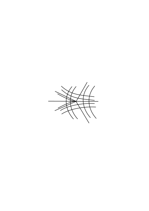
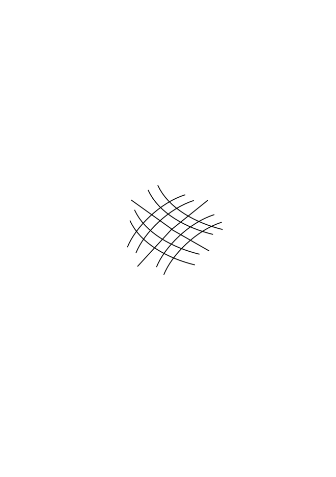
Figure 11. Axial configurations in a neighborhood of an axiumbilic point of type $E^{1}_{4,5}.$

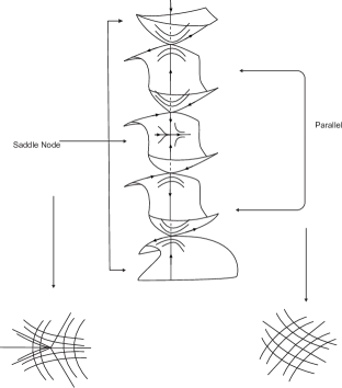
Figure 12. Lie-Cartan vector field near an axiumbilic point $E^{1}_{45}$ and the axial configuration (principal and mean).

Proof.

Condition $\alpha_{1}=\alpha_{3}=0$ implies the non-transversal contact of the curves $a_{0}=0$ and $a_{1}=0$ at the axiumbilic point $\mathfrak{p}$ expressed in the Monge chart by $(0,0)$. By Lemma 5 and Proposition 6, it is possible to express these curves as in equation (36). Assuming $\chi\neq 0$, we have the quadratic contact of the curves at the axiumbilic point.

Proposition 13 implies that over the axiumbilic point we have five equilibria of the Lie-Cartan vector field. One of them is a regular point of the Lie-Cartan surface, and this is an equilibrium of saddle-node type with center manifold transversal to the axis $p$ (see Claim 14).

The remaining equilibria are critical points of Morse type of the Lie-Cartan surface. In the neighborhood of these points, the level set ${\mathcal{G}}=0$ are locally cones, and the $4$ points are saddles of the Lie-Cartan vector field (see Claim 15).

Therefore, we conclude the configuration described in Figure 12, whose projection of the saddle-node and parallel sectors describe the principal axial and mean axial configurations close to the axiumbilic point $\mathfrak{p}$ of type $E^{1}_{45}$ (Figure 11). ∎

Proposition 17.

Let $\alpha\in{\mathcal{I}}^{r}$, $r\geq 5$, be an immersion having an axiumbilic point $\mathfrak{p}$. Then, there exist a neighborhood $V$ of $\mathfrak{p}$, a neighborhood ${\mathcal{V}}$ of ${\alpha}$ and a function $F:{\mathcal{V}}\longrightarrow\mathbb{R}$ of class ${\mathcal{C}}^{r-3}$ such that:

1. $dF_{\alpha}\neq 0$,

2. $F(\mu)=0$ if, and only if, $\mu\in{\mathcal{V}}$ has just one axiumbilic point in $V$, which is of type $E^{1}_{4,5}$,

3. $F(\mu)<0$ if, and only if, $\mu$ has exactly two axiumbilic points in $V$, one of type $E_{4}$ and the other of type $E_{5}$,

4. $F(\mu)>0$ if, and only if, $\mu$ has no axiumbilic points in $V$.

Proof.

By Proposition 13, $\alpha$ being an immersion having an axiumbilic point $\mathfrak{p}$ of type $E^{1}_{45}$, the curves $a_{0}^{\alpha}=0$ and $a_{1}^{\alpha}=0$ have quadratic contact at $\mathfrak{p}$.

Since $\frac{\partial a_{0}^{\alpha}}{\partial y}(0,0)=a_{01}\neq 0$, if follows from Implicit Function Theorem that locally, for $\mu$ in a neighborhood ${\mathcal{V}}$ of $\alpha$, $y=y_{\mu}(x)$ and $a_{0}^{\mu}(x,y_{\mu}(x))=0$.

Moreover, $\frac{\partial^{2}a_{1}^{\alpha}}{\partial x^{2}}(0,0)=b_{20}\neq 0$, and so $x=x_{\mu}$ is a local solution of $\frac{\partial a_{1}^{\mu}}{\partial x}(x_{\mu},y_{\mu}(x_{\mu}))=0$.

Define ${\mathcal{F}}(\mu)=a_{1}^{\mu}(x_{\mu},y_{\mu}(x_{\mu}))$. Consider the variation $h_{t}(x,y)=(x,y,R(x,y)+txy,S(x,y)+txy)$. It follows that $\frac{dF(t)}{dt}\bigg{|}_{t=0}\neq 0$, and so $dF_{\alpha}\neq 0$. Therefore, the result follows from the Implicit Function Theorem.

The axiumbilic point of type $E^{1}_{45}$ is therefore the transition between zero and two axiumbilic points, one of type $E_{4}$ and the other of type $E_{5}$.

In Figures 13 and 15 are illustrated this transition, with the axial configurations sketched in two different styles. See also Figure 15 for an illustration of transition in the Lie - Cartan surface.

∎

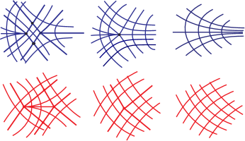
Figure 13. Axiumbilic point $E^{1}_{45}$. The axiumbilic points $E_{4}$ and $E_{5}$ collapse in an axiumbilic point $E^{1}_{45}$, and after they are eliminated and there are no axiumbilic points.

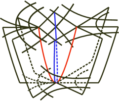
Figure 14. Bifurcation diagram of the axial configuration near an axiumbilic point of type $E^{1}_{45}$ and the structure of separatrices

Figure 15. The Lie-Cartan surface. In the left, with two axiumbilic point, in the center with four singular points, and in the right the four regular levels.

Proposition 18.

In the space of smooth mappings of $M\times\mathbb{R}\longrightarrow\mathbb{R}^{4}$ which are immersions relative to the first variable, those which have all their axiumbilic points either generic (of types $E_{3}$, $E_{4}$ and $E_{5}$) or, transversally, of types $E^{1}_{34}$ and $E^{1}_{45}$ is open and dense. Furthermore, for such families the axiumbilic points describe a regular curve in $M\times\mathbb{R}$ whose projection into $\mathbb{R}$ has only non-degenerate critical points at $E^{1}_{45}$ and the regular points of the projection is a collection of arcs bounded by $E^{1}_{34}$ points, which a the common boundary of $E_{3}$ and $E_{4}$ arcs.

Proposition 18 follow from the analyses in propositions 11 and 17 and an application of Thom Transversality Theorem to the submanifold of four jets of immersions at axiumbilic points, stratified by the generic axiumbilic points, by $E^{1}_{34}$ and type $E^{1}_{45}$, and their complement. See Section 4.

4. Transversality and Stratification

Consider the space $\mathbb{J}^{k}(M,\mathbb{R}^{4})$ of $k$-jets of immersions $\alpha$ of a compact oriented surface $M$ into $\mathbb{R}^{4}$, endowed with the structure of Principal Fiber Bundle. The base is $M$; the fiber is the space $\mathbb{R}^{4}\times\mathbb{J}^{k}(2,4)$, where $\mathcal{J}^{k}(2,4)$ is the space of $k$-jets of immersions of $\mathbb{R}^{2}$ to $\mathbb{R}^{4}$, preserving the respective origins. The structure group, $\mathbb{A}_{+}^{k}$, is the product of the group of $\mathcal{L}_{+}^{k}(2,2)$ of $k$-jets of origin and orientation preserving diffeomorphisms of $\mathbb{R}^{2}$, acting on the right by coordinate changes, and the group $\mathbb{R}^{4}\times\mathcal{O}_{+}(4,4)$ of positive isometries, acting on the left, consisting on a translation, taken as a vector in the first factor, and a positive rotation of $\mathbb{R}^{4}$, taken on the second factor. Denote by $\Pi_{k,l},k\leq l$ the projection of $\mathcal{J}^{l}(2,4)$ to $\mathcal{J}^{k}(2,4)$. It is well known that the group action commutes with projections.

Definition 19.

We define below the canonic axiumbilic stratification of $\mathcal{J}^{4}(2,4)$. The term canonic means that the strata are invariant under the action of the group $\mathbb{A}_{+}^{k}$= $\mathcal{O}_{+}(4,4)\times\mathcal{L}_{+}^{k}(2,2)$.

• aximbilic Jets: ${\mathcal{U}}^{4}$, those in the orbit of $j^{4}(x,y,R(x,y),S(x,y))$, where $R$ and $S$ are as in equations (9) and (10) satisfying the axiumbilic conditions defined in terms of $j^{2}R(0)$ and $j^{2}S(0).$ It is a closed variety of codimension $2$.

• Non-axiumbilic Jets: $(\mathcal{NU})^{4}$ is the complement of ${\mathcal{U}}^{4}$. It is an open submanifold of codimension $0$.

• Non-stable axumbilic Jets: $(\mathcal{NE})^{4}$, in the orbit of the axiumbilic jets for which:

  $\bullet$   $T=(\alpha_{1}\alpha_{4}-\alpha_{2}\alpha_{3})(r^{2}+s^{2})=0$ or

  $\bullet$   $T\neq 0$ and conditions that characterize $E_{3}$ or $E_{4}$ axiumbilic points in Proposition 8 fail.

It is a closed variety of codimension 3, which can be expressed as the union of the following invariant strata:

• Non-Transversal jets: $\mathcal{E}^{1}_{45}$ for which $T=0$ and $\chi\neq 0$. It has codimension 3.

• Transversal-double jets: $(\mathcal{E}^{1}_{34})^{4}$, The Lie-Cartan field has a quadratic saddle-node in the projective line which is characterized by Proposition 11. Has codimension 3.

• The stable axumbilic jets: $\mathcal{UE}^{4}$, the complement in $\mathcal{U}^{4}$ of $\mathcal{NE}^{4}$.

Proposition 20.

In the space of 1-parameter families of immersions, those whose 4-jet extension are transversal to the canonical axiumbilic stratification is open and dense.

Proof.

Follows from Thom Transversality Theorem [6]. ∎

5. Concluding Comments

In this work was established the principal axial and the mean axial configurations in a neighborhood of the axiumbilc points of types $E^{1}_{34}$ and $E^{1}_{45}$. The approach concerning methods and class of differentiability requirements is distinct from that presented in the work of Gutiérrez-Guínez-Castañeda in [3]. The use of the Lie-Cartan suspension method made possible the study of these points by means the classic theory of differential equations, in clear analogy with the saddle-node bifurcation of vector fields in the plane, following [1], [10] and [5].

The type $E^{1}_{34}$ satisfies the transversality condition of the curves $a_{0}$ and $a_{1}$, Proposition 6, which amounts to the fact the Lie-Cartan surface remains regular in a neighborhood of the projective axis over the axiumbilic point. In this case there is a saddle-node equilibrium point of the Lie-Cartan vector field whose central separatrix is along the projective axis itself. The axial configurations are established in Proposition 10 and the qualitative change (bifurcation) between the types $E_{3}$ and $E_{4}$, with the variation of a one parameter in the space of immersions, is explained in Proposition 7. See Figure 10.

In the case $E^{1}_{45}$ the transversality condition fails, since curves $a_{0}$ and $a_{1}$, Proposition 13, have quadratic contact at the axiumbilic point. Here the Lie-Cartan surface is not regular along the projective axis. It is established in Proposition 13 that there are four conic critical points of Morse type on the $p-$axis. At these points there are partially hyperbolic equilibria of the Lie-Cartan vector field. There is also a saddle-node equilibrium in the regular part of the surface whose central separatrix is transversal to the projective axis. The integral curves of the Lie - Cartan vector field on the regular components of the Lie - Cartan (which are four bi-punctured disks) are illustrated in Figure 12. Their projections on the plane give the axial configurations in a neighborhood of the axiumbilic point.

In Proposition 18 is established the one parameter variation (bifurcation) in the space of immersions. This leads to the fact that for small perturbations of an immersion with an axiumbilic point of this type it holds that two axiumbilic points, one of type $E_{4}$ and the other of type $E_{5}$, bifurcate form $E^{1}_{45}$ or disappear leaving a neighborhood free from axiumbilic points, in full analogy with the saddle-node bifurcation [1] and [10]. See Figure 14.

In Theorem 20 the genericity of the points $E^{1}_{34}$ and $E_{45}^{1}$ is established in terms of stratification and transversality.

Ronaldo Garcia
Instituto de Matemática e Estatística
Universidade Federal de Goiás,
CEP 74001–970, Caixa Postal 131
Goiânia, Goiás, Brazil

Jorge Sotomayor
Instituto de Matemática e Estatística
Universidade de São Paulo,
Rua do Matão 1010, Cidade Univeritária, CEP 05508-090,
São Paulo, S. P, Brazil

Flausino L. Spindola
Instituto de Matemática e Estatística
Universidade de São Paulo,
Rua do Matão 1010, Cidade Univeritária, CEP 05508-090,
São Paulo, S. P, Brazil

References

[1] Andronov, A. Gordon, I. Leontovich, E. Maier, G. Theory of Bifurcations of Dynamical Systems on a Plane. Israel Program for Scientific Translations, John Wiley, New York, 1973.
[2] Gutiérrez, C., Guíñez, V. Simple Umbilic Points on Surfaces Immersed in . Discrete Contin. Dyn. Syst. 9 (2003), 877-900.
[3] Gutiérrez, C., Guíñez V., Castañeda, A. Quartic Differential Forms and Transversal Nets with Singularities. Discrete Contin. Dyn. Syst.26 (2010), 225-249.
[4] Gutiérrez, C., Guadalupe, I., Tribuzy, R., Guíñez, V. Lines of Curvature on Surfaces immersed in . Bol. Soc. Bras. Mat., 28 (1997), 233-251.
[5] Gutiérrez, C., Garcia, R. , Sotomayor, J. Bifurcations of Umbilic Points and Related Principal Cycles. Journ. Dyn. and Diff. Eq., 16 (2004), 321-346.
[6]H.T. Levine,
Singularities of Differentiable Mappings, Lect. Notes in Math. 192,
1971.
[7] Little, J. A. On Singularities of Submanifolds of Higher Dimensional Euclidean Spaces. Ann. Mat. Pura Appl., 83 (1969), 261-335.
[8] Mello, L. F. Mean Directionally Curved Lines on Surfaces Immersed in . Publ. Mat., 47,(2003), 415-440.
[9] Mello, L. F. Orthogonal asymptotic lines on surfaces immersed in . Rocky Mountain J. Math. 39 (2009), 1597-1612.
[10] Sotomayor, J. Generic one-parameter families of vector fields on two-dimensional manifolds. Inst. Hautes Études Sci. Publ. Math. 43 (1974), 5-46.
[11] Sotomayor, J., Garcia, R. Lines of Axial Curvature on Surfaces Immersed in . Diff. Geom. and its Applications. 12 (2000), 253-269.
[12] Sotomayor, J., Garcia, R. Differential Equations of Classical Geometry, a Qualitative Theory. Publicações Matemáticas. IMPA. 2009.