Electrical current and coupled electron-nuclear spin dynamics in double quantum dots

Abstract

We examine electronic transport in a spin-blockaded double quantum dot. We show that by tuning the strength of the spin-orbit interaction the current flowing through the double dot exhibits a dip at zero magnetic field or a peak at a magnetic field for which the two-electron energy levels anticross. This behaviour is due to the dependence of the singlet-triplet mixing on the field and spin-orbit amplitude. We derive approximate expressions for the current as a function of the amplitudes of the states involved in the transport. We also consider an alternative model that takes into account a finite number of nuclear spins and study the resulting coupled dynamics between electron and nuclear spins. We show that if the spin ensemble is in a thermal state there are regular oscillations in the transient current followed by quasi-chaotic revivals akin to those seen in a thermal Jaynes-Cummings model.

I Introduction

A double quantum dot (DQD) can be used for the detailed investigation of spin interactions among electron spins and even between electron and nuclear spins. The interactions can be probed optically or electrically by monitoring the electrical current flowing through the DQD as a function of the energy offset between the two dots and the applied magnetic field. In a spin-blockaded DQD, the current through the DQD is large when the two electrons form a singlet state, whereas it is suppressed when the two electrons form a triplet state. ono The spin blockade mechanism is due to the Pauli principle and has been demonstrated in semiconductor heterostructure quantum dots ono as well as carbon nanotube dots. buitelaar It has also been shown that the transient behaviour of the leakage current can provide valuable information about the interactions between electrons in the DQD and nuclear spins in the host material. ono2004 In particular, the electrical transport process can lead to a coupled electron-nuclear dynamics, nuclear spin polarization, and hysteresis effects. ono ; ono2004 ; abolfath

In the spin blockade regime, the small leakage current increases when there is a process that leads to singlet-triplet hybridization (mixing). A non spin-conserving interdot tunnelling is one such process. This type of tunnelling may result from a spin-orbit interaction (SOI), which in some cases can be strong enough and thus has to be taken into account. pfund ; perge The hyperfine interaction (HI) between dot electrons and nuclear spins can also lead to singlet-triplet hybridization. In a simplified approach, the nuclear spins create an effective magnetic field which acts on the electron spins. This field can point in an arbitrary direction and mixes singlet and triplet states.

The electrical current in a DQD system has been examined theoretically in the presence of strong SOI and in the regime where the coupling of the DQD to the leads corresponds to the largest rate in the system. danon2009 In the first part of this work, we consider a DQD weakly coupled to the leads and examine the current in the resonant regime, i.e., when the lowest singlet and triplet energy levels are almost aligned. Unlike the approach followed in Ref. danon2009, we consider explicitly the lowest one-electron states and derive rate equations that involve the transition rates between one- and two-electron states. The SOI is modelled with a non spin-conserving tunnel coupling amplitude $t_{\mathrm{so}}$ between the two dots danon2009 ; romeo which couples the triplet states $|T_{+}\rangle$, $|T_{-}\rangle$ with singlet states. We consider weak SOI, that is $t_{\mathrm{so}}<t_{\mathrm{c}}$, where $t_{\mathrm{c}}$ is the spin-conserving interdot tunnel coupling. The effect of a strong SOI on a spin-blockaded DQD has been investigated in Ref. danon2009, with a more general SOI model in which all triplet states couple to singlet states. Further, we here give emphasis to the regime where the HI is weak enough or absent, which might be the case in carbon-based quantum dots. rozhkov ; chorley The main aim of the first part of this work is to determine the current as a function of the amplitudes of the one- and two-electron states which participate in the transport cycle. Some approximate results which give valuable insight into the basic behavior of the current are derived. We show that, depending on the strength of the SOI, the current shows a dip at zero magnetic field or a peak when the lowest two-electron energy levels anticross. This behaviour occurs because when $t_{\mathrm{so}}$ is large the singlet-triplet mixing near zero field is much weaker compared to that at high field. This gives rise to a dip at zero field. However, when $t_{\mathrm{so}}$ is small the mixing is strong only near the anticrossing point leading to a peak in the current.

In the second part of this work we focus mostly on the interplay between SOI and HI. To properly account for the HI, we employ a microscopic ‘toy’ model which takes into account a finite number of nuclear spins. To make this model tractable, only the two lowest singlet-triplet states are considered, and we treat the nuclear spins as a single large spin. We first consider the interplay between the SOI and HI, and its effect on the steady state transport and nuclear spin polarization. We find a sharp transition in the current and polarization as the SOI is increased, consistent with the topological phase transition investigated in Ref. Rudner10, . Second, we look at the transient dynamics induced by the HI alone, and find a strong oscillatory contribution depending on the hyperfine coupling strength and inversely proportional to the square root of the number of nuclear spins.

II Electrical current in the spin blockade regime

II.1 Physical Model

In this section the electrical current through the DQD is examined when the electron-nuclear spin dynamics are uncoupled. This section is concerned with the effect of the SOI on the electrical current while HI-induced effects due to the coupled electron-nuclear dynamics are addressed in the next section. The DQD is modelled with the two-site Hamiltonian

$$H_{\mathrm{DQD}}=H_{\mathrm{c}}+H_{\mathrm{so}}+H_{\mathrm{hf}}+\sum_{i=1}^{2}\varepsilon_{i}n_{i}+U\sum_{i=1}^{2}n_{i\uparrow}n_{i\downarrow}+\frac{\Delta}{2}\sum_{i=1}^{2}\sigma_{i}^{\mathrm{z}}.$$ (1)

Here $H_{\mathrm{c}}$ is the tunnel-coupling Hamiltonian that conserves spin and has the form

$$H_{\mathrm{c}}=-t_{\mathrm{c}}(c^{\dagger}_{1\uparrow}c_{2\uparrow}+c^{\dagger}_{1\downarrow}c_{2\downarrow})+\mathrm{H.c.},$$ (2)

and the Hamiltonian part due to the SOI that allows spin-flip has the form romeo

$$H_{\mathrm{so}}=-t_{\mathrm{so}}(c^{\dagger}_{1\uparrow}c_{2\downarrow}-c^{\dagger}_{1\downarrow}c_{2\uparrow})+\mathrm{H.c.}.$$ (3)

For the HI we assume the form jouravlev

$$H_{\mathrm{hf}}=\frac{1}{2}g_{\mathrm{e}}\mu_{\mathrm{B}}({\bf B}_{\mathrm{N},1}\bm{\sigma}_{1}+{\bf B}_{\mathrm{N},2}\bm{\sigma}_{2}).$$ (4)

The operator $c_{i\sigma}^{\dagger}$ ($c_{i\sigma}$) creates (destroys) an electron on dot $i=1,2$ with spin $\sigma=\{\uparrow,\downarrow\}$ and orbital energy $\varepsilon_{i}$. The number operator is denoted by $n_{i}=\sum_{\sigma}n_{i\sigma}=c_{i\uparrow}^{\dagger}c_{i\uparrow}+c_{i\downarrow}^{\dagger}c_{i\downarrow}$. The tunnel coupling amplitude between the two dots is $t_{\mathrm{c}}$, the amplitude due to the SOI is $t_{\mathrm{so}}$, the charging energy is $U$, and $\Delta=g_{\mathrm{e}}\mu_{\mathrm{B}}B$ is the Zeeman splitting due to the external magnetic field $B$ in the $z$-direction. Here ${\bf B}_{\mathrm{N},i}$ is the magnetic field in the $i$th dot due to the nuclear spins and $\bm{\sigma}_{i}$ are the Pauli operators.

The quantum states which participate in the transport cycle in the spin blockade regime are the 2 lowest one-electron states and the 5 lowest two-electron states. For simplicity the three-electron states are neglected in this study because they do not change qualitatively the basic results. The one-electron eigenstates $|j;n=1\rangle$ can be written in the general form

$$|j;1\rangle=\alpha_{j}|\uparrow,0\rangle+\beta_{j}|0,\uparrow\rangle+\gamma_{j}|\downarrow,0\rangle+\delta_{j}|0,\downarrow\rangle,$$ (5)

with $j=1,2$ and $c^{\dagger}_{1\sigma}|0\rangle=|\sigma,0\rangle$, $c^{\dagger}_{2\sigma}|0\rangle=|0,\sigma\rangle$. Here the eigenstates are ordered with increasing energy. In the spin-blockade regime $U\gg t_{\mathrm{c}}$ and further there is an energy offset between the two dots. In this work we choose for the on site energies $\varepsilon_{2}=\varepsilon_{1}-U/2$ and define the energy detuning as $\delta=E(1,1)-E(0,2)$, where $E(n,m)$ is the energy of the charge state which has $n$ $(m)$ electrons on dot $i=1$ ($i=2$). If $H_{\mathrm{so}}=0$ and $H_{\mathrm{hf}}=0$ then $\alpha_{1}=\beta_{1}=0$ and $\gamma_{2}=\delta_{2}=0$ and the nonzero amplitudes satisfy $\delta_{1}\gg\gamma_{1}$ and $\beta_{2}\gg\alpha_{2}$. When $H_{\mathrm{so}}\neq 0$ the amplitudes $\alpha_{1}$, $\beta_{1}$, $\gamma_{2}$, $\delta_{2}$ are in general nonzero and satisfy $\beta_{1}\ll\alpha_{1}$, $\delta_{2}\ll\gamma_{2}$.

Neglecting double occupation on dot 1, a two-electron eigenstate $|j;n=2\rangle$ with $j=3,...7$ has the general form

$$|j;2\rangle=a_{j}|\uparrow,\uparrow\rangle+b_{j}|\uparrow,\downarrow\rangle+c_{j}|\downarrow,\uparrow\rangle+d_{j}|\downarrow,\downarrow\rangle+e_{j}|0,\uparrow\downarrow\rangle.$$ (6)

Here $|T_{-}\rangle=|\downarrow,\downarrow\rangle=c^{\dagger}_{1\downarrow}c^{\dagger}_{2\downarrow}|0\rangle$, $|T_{+}\rangle=|\uparrow,\uparrow\rangle=c^{\dagger}_{1\uparrow}c^{\dagger}_{2\uparrow}|0\rangle$, $|\sigma,\sigma^{\prime}\rangle=c^{\dagger}_{1\sigma}c^{\dagger}_{2\sigma^{\prime}}|0\rangle$, and $|S_{02}\rangle=|0,\uparrow\downarrow\rangle=c^{\dagger}_{2\uparrow}c^{\dagger}_{2\downarrow}|0\rangle$. The amplitudes of the various components depend on the strengths of the SOI and HI as well as the Zeeman splitting and detuning. When $H_{\mathrm{so}}=0$ and $H_{\mathrm{hf}}=0$ the two-electron eigenstates correspond to the triplet states $|T_{+}\rangle$, $|T_{-}\rangle$, $|T_{0}\rangle=(|\uparrow\downarrow\rangle+|\downarrow\uparrow\rangle)/\sqrt{2}$ and the two singlet states, which consist of the components $|S_{02}\rangle=|0,\uparrow\downarrow\rangle$ and $|S_{11}\rangle=(|\uparrow\downarrow\rangle-|\downarrow\uparrow\rangle)/\sqrt{2}$. The effect of the $H_{\mathrm{so}}$ is to couple the $|T_{+}\rangle$, $|T_{-}\rangle$ states to singlet components. As shown below the coupling strength increases with $t_{\mathrm{so}}$ and, for a fixed detuning, is sensitive to the Zeeman splitting.

To calculate the electrical current flowing through the DQD we employ a density matrix approach within the Born and Markov approximations. gardiner The internal parameters of the DQD and the chemical potentials of the two leads are adjusted to the spin-blockade regime. This regime can be identified from the fact that when $H_{\mathrm{so}}=0$ and $H_{\mathrm{hf}}=0$ the three triplet states $|T_{+}\rangle$, $|T_{-}\rangle$, and $|T_{0}\rangle$ are equally and almost fully populated ($\sim 1/3$), provided spin decoherence is ignored, and the current as a function of the source-drain bias is suppressed.

II.2 Results

When $t_{\mathrm{so}}$ is nonzero the $|T_{+}\rangle$, $|T_{-}\rangle$ states couple to singlet states and this coupling has a direct effect on the current. To demonstrate this effect we show in Fig. 1 the current as a function of the Zeeman splitting $\Delta$ and energy detuning $\delta$ between the two dots when there is no HI. The coupling of the states is strong near the anti-crossing points leading to an increase in the current (see also below). As a result the curves of high current map-out the points where the energy levels of the quasi singlet and triplet states anticross. When $t_{\mathrm{so}}=0$ the leakage current is approximately constant and no high current curves occur.

To understand the role of the SOI we show in Fig. 2 the energy diagram of the two-electron states as well as the current as a function of the Zeeman splitting $\Delta$, for a fixed energy detuning $\delta$ and different SOI amplitudes with $H_{\mathrm{hf}}=0$. We concentrate on the regime $t_{\mathrm{so}}<t_{\mathrm{c}}$ and choose $\delta<0$, which is experimentally the most interesting case for spin-qubit applications ono ; chorley ; petta , because the spin pair can be described by an effective Heisenberg model. The resonant current that is defined as the current at the anticrossing point increases with $t_{\mathrm{so}}$ and the same occurs for the asymptotic current that is defined as the current at a high magnetic field. Therefore, when $t_{\mathrm{so}}$ is large enough the asymptotic current becomes approximately equal to the resonant current and thus the peak cannot be distinguished. The same pattern occurs when the direction of the magnetic field is reversed, thus the current as a function of the Zeeman splitting shows a dip at $\Delta=0$. To a good approximation this pattern is independent of the detuning, provided $t_{\mathrm{so}}$ is large, and consequently the anticrossing points of the energy diagram cannot be probed.

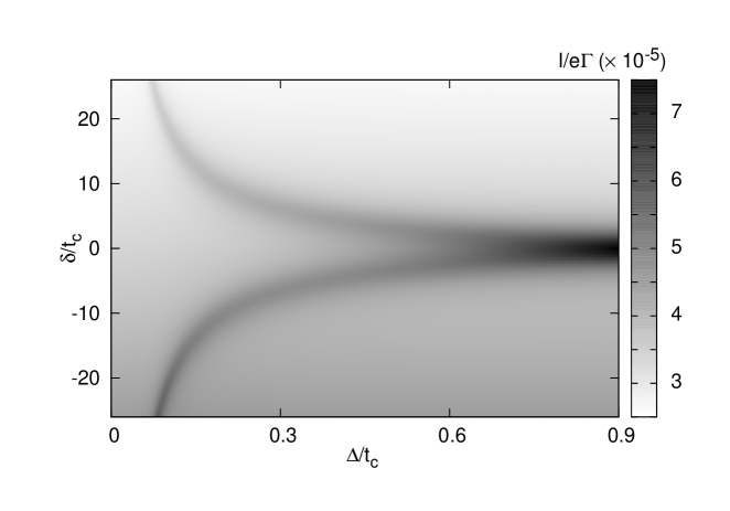
Figure 1: Electrical current, $I$, as a function of the Zeeman splitting, $\Delta$, and energy detuning, $\delta$, when there is no hyperfine interaction. The SOI amplitude is $t_{\mathrm{so}}=0.01t_{\mathrm{c}}$, where $t_{\mathrm{c}}$ is the spin-conserving interdot tunnel coupling.

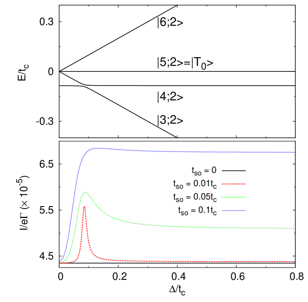
Figure 2: (Color online) The top panel shows the energies, $E$, of the four lowest two-electron states as a function of the Zeeman splitting, $\Delta$, for an energy detuning $\delta=-25t_{\mathrm{c}}$ and SOI amplitude $t_{\mathrm{so}}=0.1t_{\mathrm{c}}$, where $t_{\mathrm{c}}$ is the spin-conserving interdot tunnel coupling. The notation of the states is given in the main text in Eq. (6). The bottom panel shows the electrical current, $I$, as a function of the Zeeman splitting $\Delta$ for an energy detuning $\delta=-25t_{\mathrm{c}}$.

To quantify the above results we analyze the rate equations and calculate analytically the transition rates. Then we derive the steady-state current for some interesting limits, such as for example the current at the singlet-triplet anticrossing point, as well as for $B\sim 0$ and $B$ high. We are interested in determining the current in the steady-state for a DQD that is weakly coupled to the leads. In this regime we can consider only the diagonal elements of the density matrix newreference and the dynamics of the system is described by the rate equations

$$\frac{d\rho_{n}}{dt}=-\rho_{n}\sum_{m}R_{nm}+\sum_{m}\rho_{m}R_{mn},$$ (7)

where the diagonal elements of the density matrix are denoted by $\rho_{n}=\rho_{nn}$ and the normalization condition is $\sum^{7}_{n=1}\rho_{n}=1$. The transition rate from an eigenstate $|n\rangle$ of the DQD with eigenenergy $E_{n}$ to an eigenstate $|m\rangle$ with eigenenergy $E_{m}$ is

$$R_{nm} = \Gamma\sum_{\sigma}[|\langle n|c_{1\sigma}|m\rangle|^{2}f_{L}(E_{mn})+|\langle m|c_{1\sigma}|n\rangle|^{2}f^{-}_{L}(E_{nm})$$ (8)

$$+ |\langle n|c_{2\sigma}|m\rangle|^{2}f_{R}(E_{mn})+|\langle m|c_{2\sigma}|n\rangle|^{2}f^{-}_{R}(E_{nm})],$$

where $\Gamma=2\pi|t_{r}|^{2}D_{r}/\hbar$. The tunnelling amplitude between dot and lead is $t_{r}$, $f_{\ell}(E_{mn})$ is the Fermi-Dirac distribution function at chemical potential $\mu_{\ell}$, with $E_{mn}=E_{m}-E_{n}$ and $f^{-}=1-f$. Also, $D_{r}$ is the density of states for the leads, which we assume to be constant and equal for both leads.

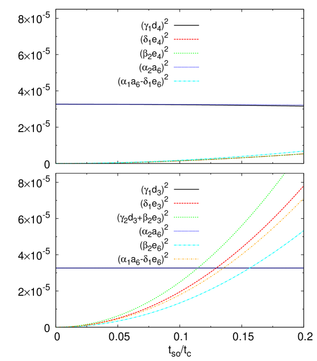
Figure 3: (Color online) The figure shows the important quantities which determine the transition rates through the parameters $F_{0}$, $E_{0}$ (top panel) and $F_{a}$, $E_{a}$ (bottom panel) defined in Eqs. (14), (15) and Eqs. (20), (21) respectively. The energy detuning is $\delta=-25t_{\mathrm{c}}$ and the Zeeman splitting is chosen in the low field regime $\Delta=0.02t_{\mathrm{c}}$ (top) and asymptotic regime $\Delta=0.7t_{\mathrm{c}}$ (bottom).

The operator for the electrical current, for example, for the right lead is

$$\hat{I}=\frac{e}{\hbar}i\sum_{k\sigma}t_{r}(c^{\dagger}_{2\sigma}d_{{k}\sigma}-d^{\dagger}_{{k}\sigma}c_{2\sigma}),$$ (9)

where $d_{{k}\sigma}$ denotes a lead operator. Tracing out the leads we derive the following expression for the average current

$$I=e\Gamma\sum_{nm\sigma}\rho_{n}[|\langle n|c_{2\sigma}|m\rangle|^{2}f_{R}(E_{mn})-|\langle m|c_{2\sigma}|n\rangle|^{2}f^{-}_{R}(E_{nm})].$$ (10)

Starting with the rate equations and calculating the transition rates it can be readily derived that the absolute value of the current for $H_{\mathrm{hf}}=0$ is $I=e\sum^{7}_{n=3}(R_{n1}+R_{n2})\rho_{n}$. The simplest regime is when $t_{\mathrm{so}}=0$ and $B=0$. Here, the occupations of the triplet states satisfy $\rho_{4}=\rho_{5}=\rho_{6}=\rho_{T}$. From the steady-state condition, $d\rho_{n}/dt=0$, it can be derived that

$$3\rho_{T}\approx 1-\left(\frac{R_{14}}{R_{41}+R_{42}}+\frac{R_{15}}{R_{51}+R_{52}}+\frac{R_{16}}{R_{61}+R_{62}}\right)^{-1}.$$ (11)

For weakly coupled dots the second term is typically negligible and $\rho_{T}\approx 1/3$. It is easy to prove that this approximation is excellent when $t_{c}$ is small and $\delta$ is large. In this regime the leakage current is

$$I_{T}\approx 2e\Gamma\left(\frac{R_{14}}{R_{41}+R_{42}}+\frac{R_{15}}{R_{51}+R_{52}}+\frac{R_{16}}{R_{61}+R_{62}}\right)^{-1}.$$ (12)

For $t_{\mathrm{so}}\neq 0$ we calculate analytically the transition rates and derive that for low magnetic fields the current is given approximately by the expression

$$I_{0}\approx\frac{2e\Gamma}{\frac{1}{2}F_{0}+\frac{1}{2}E_{0}},$$ (13)

where

$$E_{0}=\frac{1}{(\gamma_{1}d_{4})^{2}+(\delta_{1}e_{4})^{2}+(\beta_{2}e_{4})^{2}}+\frac{R_{15}}{R_{51}+R_{52}},$$ (14)

$$F_{0}=\frac{1}{(\alpha_{2}a_{6})^{2}+(\alpha_{1}a_{6}-\delta_{1}e_{6})^{2}}+\frac{R_{25}}{R_{51}+R_{52}}.$$ (15)

The transition rates $R_{15}$, $R_{25}$ involve the one-electron state $|1;1\rangle$, $|2;1\rangle$ respectively, and the triplet state $|T_{0}\rangle=|5;2\rangle$. The terms which are proportional to $R_{12}$, $R_{25}$ do not affect the physics we examine here, so for this reason they are not given explicitly. Also, as seen in Fig. 2, in the small $t_{\mathrm{so}}$ regime that we are interested in $I_{0}$ is to a good approximation independent of $t_{\mathrm{so}}$. An approximate expression for the resonant current is

$$I_{r}\approx\frac{2e\Gamma}{\frac{2}{3}F_{r}+\frac{1}{3}E_{r}},$$ (16)

with the parameters

$$E_{r}=\frac{1}{(\gamma_{1}d_{4})^{2}+(\delta_{1}e_{4})^{2}+(\beta_{2}e_{4})^{2}}+\frac{R_{15}}{R_{51}+R_{52}},$$ (17)

$$F_{r}=\frac{1}{(\alpha_{2}a_{6})^{2}+(\beta_{2}e_{6})^{2}+(\alpha_{1}a_{6}-\delta_{1}e_{6})^{2}}+\frac{R_{25}}{R_{51}+R_{52}}.$$ (18)

The resonant current corresponds to the magnetic field $B_{r}$ for which the lowest quasi singlet and triplet states anticross and it is well-defined for $t_{\mathrm{so}}\ll t_{\mathrm{c}}$. The asymptotic current that corresponds to a high $B$ is given approximately by the expression

$$I_{a}\approx\frac{2e\Gamma}{\frac{1}{2}F_{a}+\frac{1}{2}E_{a}},$$ (19)

with

$$E_{a}=\frac{1}{(\gamma_{1}d_{3})^{2}+(\delta_{1}e_{3})^{2}+(\gamma_{2}d_{3}+\beta_{2}e_{3})^{2}}+\frac{R_{15}}{R_{51}+R_{52}},$$ (20)

$$F_{a}=\frac{1}{(\alpha_{2}a_{6})^{2}+(\beta_{2}e_{6})^{2}+(\alpha_{1}a_{6}-\delta_{1}e_{6})^{2}}+\frac{R_{25}}{R_{51}+R_{52}}.$$ (21)

The asymptotic current is defined at a high magnetic field where the current varies slowly with $B$.

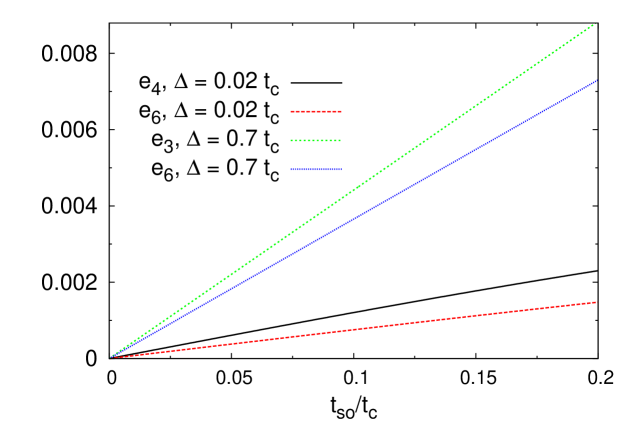
Figure 4: (Color online) The figure shows the absolute amplitudes $e_{3}$, $e_{4}$ and $e_{6}$ which express the mixing of the triplets $|T_{+}\rangle$ and $|T_{-}\rangle$ with the $|S_{02}\rangle$ state. The Zeeman splitting is chosen in the low field regime $\Delta=0.02t_{\mathrm{c}}$ and asymptotic regime $\Delta=0.7t_{\mathrm{c}}$.

Equation (13) can be used to estimate the width of the current peak that occurs at $\Delta_{r}=g_{e}\mu_{B}B_{r}$. Specifically, if we denote by $\Delta_{r}-\Delta_{1}$ the half width at half maximum of the peak, then $\Delta_{1}$ satisfies the relation $I_{0}(\Delta_{1})=I_{r}/2$. In the same way the width of the $\Delta=0$ minimum can be estimated in the regime $I_{a}\sim I_{r}$. If $\Delta_{1}$ corresponds to half of the width then to a good approximation it has to satisfy the relation $I_{0}(\Delta_{1})=I_{a}/2$.

The variation of the current as a function of the magnetic field and SOI strength is mainly due to the change of the first terms in $E_{i}$ and $F_{i}$. For example, if $t_{\mathrm{so}}\ll t_{\mathrm{c}}$, then as can be seen in Fig. 3 only the quantities $(\gamma_{1}d_{4})^{2}$, $(\alpha_{2}a_{6})^{2}$, and $(\gamma_{1}d_{3})^{2}$ which contribute to $E_{i}$ and $F_{i}$ are important. Because these quantities are approximately equal we derive that $E_{a}\approx E_{0}$ and $F_{a}\approx F_{0}$, thus $I_{a}\sim I_{0}$. In the same way, at $B_{r}$ the corresponding amplitudes in Eqs. (17) and (18) lead to $E_{0}>E_{r}$ and $F_{0}>F_{r}$. Thus, $I_{r}>I_{0}$ and a peak is formed at $B_{r}$. On the other hand, in the range $t_{\mathrm{so}}<t_{\mathrm{c}}$ the quantities $(\delta_{1}e_{3})^{2}$, $(\gamma_{2}d_{3}+\beta_{2}e_{3})^{2}$, and $(\beta_{2}e_{6})^{2}$, $(\alpha_{1}a_{6}-\delta_{1}e_{6})^{2}$ increase drastically (Fig. 3). As a result, $E_{a}$ and $F_{a}$ decrease significantly, whereas $E_{0}$ and $F_{0}$ do not change a lot. Therefore, for intermediate or large $t_{\mathrm{so}}$ the asymptotic current $I_{a}$ is much larger than the current at very low fields and it approaches the current $I_{r}$. Eventually as $t_{\mathrm{so}}$ increases the current shows a dip for $\Delta=0$.

Inspection of the various amplitudes involved in the transition rates demonstrates that the important amplitudes in order to understand the current are the $e_{4}$ (or $e_{3}$ when $B$ is high) and $e_{6}$. These amplitudes express the mixing of the $|T_{+}\rangle$ and $|T_{-}\rangle$ states with the $|S_{02}\rangle$ component. These amplitudes are responsible for the behaviour of the current when $t_{\mathrm{so}}$ is included in the model. As shown in Fig. 4, when $t_{\mathrm{so}}$ is not too small the mixing of the $|T_{+}\rangle$, $|T_{-}\rangle$ states with the $|S_{02}\rangle$ component is stronger in the asymptotic regime than for $B\sim 0$. For this reason the current is more sensitive to $t_{\mathrm{so}}$ when $B$ is high but shows only a small variation with $t_{\mathrm{so}}$ for $B\sim 0$. Furthermore, as B increases (in the asymptotic regime) then for a fixed $t_{\mathrm{so}}$ and negative detuning the amplitude $e_{6}$ for the $|T_{+}\rangle$ state increases, whereas the amplitude $e_{3}$ for the $|T_{-}\rangle$ state decreases. This behaviour can be understood by noticing that the corresponding anticrossing points move along the detuning axis in opposite directions. In Eq. (19), $E_{a}+F_{a}$ is to a good approximation constant and the current $I_{a}$ remains constant as $\Delta$ increases.

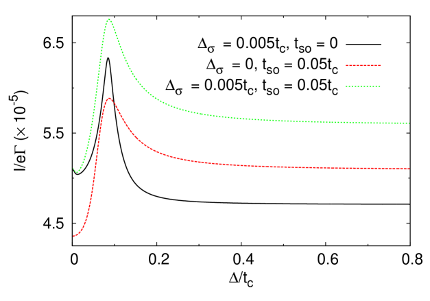
Figure 5: (Color online) Electrical current, $I$, as a function of the Zeeman splitting, $\Delta$, for the energy detuning $\delta=-25t_{\mathrm{c}}$ and different combinations of SOI and HI strengths. Here $\Delta_{\sigma}=g_{\mathrm{e}}\mu_{\mathrm{B}}\sigma_{\mathrm{N}}$.

To take into account the hyperfine interaction, we follow a standard approach and treat the nuclear magnetic fields ${\bf B}_{\mathrm{N},i}$ in the two dots as quasi-static classical variables which take random values. jouravlev In this case the electron and nuclear spin dynamics are uncoupled. In the next section we develop a model to look at the coupled dynamics. The distribution for each random static field is Gaussian with spread $\sigma_{\mathrm{N}}$. The electrical current is computed as the average over different random field configurations. jouravlev This is a good approximation when the nuclear dynamics is much slower than the electron dynamics. In Fig. 5 we plot the current versus Zeeman splitting. When $t_{\mathrm{so}}=0$, a peak is formed at the singlet-triplet anticrossing point due to the mixing caused now by the HI. When both $t_{\mathrm{so}}$ and $\sigma_{\mathrm{N}}$ are nonzero the resonant and the asymptotic current increase. However, for $\Delta=0$ the current is determined by the HI, consistent with the results in Ref. danon2009, . As the spread $\sigma_{\mathrm{N}}$ increases, the HI results in a peak at $\Delta=0$, though the $\Delta=0$ current may have a more complicated form when $\sigma_{\mathrm{N}}$ is large. In the small $\sigma_{\mathrm{N}}$ regime that we are interested in and for $t_{\mathrm{so}}\neq 0$, the $\Delta=0$ current is typically smaller than the asymptotic current. Our numerical calculations confirm that these trends occur for different choices of $t_{\mathrm{so}}$ provided that $g_{\mathrm{e}}\mu_{\mathrm{B}}\sigma_{\mathrm{N}}\ll t_{\mathrm{so}}$.

III Nuclear spin polarization and transient dynamics

III.1 Physical model

The model employed in the previous section provides insight into the current, but it does not capture the coupled electron-nuclear spin dynamics. Thus, for example, the nuclear spin polarization as a result of the transported electrons through the DQD cannot be examined. In this section we look at the DQD system from a different perspective. Specifically, we use an idealized model to study the coupled electron-nuclear spin dynamics and how this affects the transient behaviour of the current. We will use this model to show two things. First, that the presence of even a weak spin-orbit coupling can prevent nuclear spin polarization. Second, if the nuclear spin state is completely thermalized several interesting features arise in the transient electron current; regular beating followed by quasi-chaotic oscillations.

A true model of the $2^{N}$ states which describe the $N$ nuclear spins is computationally intractable, but some insight can be gained from, e.g., treating the nuclear spins as a “giant” spin. Rudner10 ; Brandes ; Inoshita2002 ; Inoshita2004 In addition to reduce the complexity even further, we restrict ourselves to a small subspace of the two-electron Hilbert space, spanned by the states $|T_{+}\rangle$, $|S_{11}\rangle$, and $|S_{02}\rangle$. This is a reasonable approximation under an appropriate bias, i.e., when only the state $|T_{+}\rangle$ is in the voltage bias window (and neglecting tunneling, from the reservoirs, into superpositions of the singlet states). In addition we assume that the rate of tunneling from the left lead to the dot is large, and that we are at the anti-crossing point of the singlet-triplet states. danon2009 This reduction of the state-space does also neglect the occupation of the $|0,\downarrow\rangle$ state, and trapping in other single-electron-occupation states. As a test, we included the single-electron state, $|0,\downarrow\rangle$, in an extended model, but it had little impact on the results we present here. Thus hereafter it will be neglected. In addition, another interesting regime to investigate would be to assume a larger bias and include all three triplet states. However, since all the interesting coupled electron-nuclear effects we discuss here are mediated by the $|T_{+}\rangle$ and $|S_{11}\rangle$ dynamics, such a regime may only reduce the visibility of these effects.

We model the interaction of these three states with a non-equilibrium master equation. This model allows a flow of electrons through the DQD, and thus we can estimate properties like the total polarization of the nuclear spin, and the transient dynamics of the coupled electron-nuclear spin system. This is in contrast to treating the spins as a frozen spin bath, Rosen as a semi-classical degree of freedom, Brandes ; Rudner2011 or as a non-Markovian environment. Ru

The total Hamiltonian of the system is then written as

$$H=H_{\mathrm{c}}+H_{\mathrm{so}}+H_{\mathrm{hf}}-\Delta|T_{+}\rangle\langle T_{+}|-\delta|S_{02}\rangle\langle S_{02}|,$$ (22)

where $H_{\mathrm{c}}$ describes the coupling between the singlet states

$$H_{\mathrm{c}}=t_{\mathrm{c}}\big{[}|S_{11}\rangle\langle S_{02}|+|S_{02}\rangle\langle S_{11}|\big{]},$$ (23)

and $H_{\mathrm{so}}$ is the Hamiltonian part due to the SOI, which couples singlet-triplet states, and has the form

$$H_{\mathrm{so}}=t_{\mathrm{so}}\big{[}|T_{+}\rangle\langle S_{02}|+|S_{02}\rangle\langle T_{+}|\big{]}.$$ (24)

The hyperfine interaction is

$${H_{\mathrm{hf}}=\frac{g}{2}\sum_{k=1}^{N}\left[|T_{+}\rangle\langle T_{+}|I_{z}^{k}+\frac{1}{\sqrt{2}}\left\{\sigma^{(1)}_{-}I_{+}^{k}+\sigma^{(1)}_{+}I_{-}^{k}\right\}\right]}.$$ (25)

Here $\delta$ is the energy detuning and $\Delta=g_{e}\mu_{B}B$ is the Zeeman splitting caused by the external magnetic field $B$ in the $z$-direction, $t_{\mathrm{so}}$ is the spin-orbit coupling, and $t_{\mathrm{c}}$ is the coherent tunnelling amplitude for the singlets. In $H_{\mathrm{hf}}$ we use an effective-spin notation so that $\sigma^{(1)}_{+}=|T_{+}\rangle\langle S_{11}|$. The coupling $g$ is the nuclear hyperfine coupling term, $g=A/N$, where $N$ is the number of nuclear spins and $A$ is in the range of 80 $\mu$eV.

For simplicity, we assume the nuclear spins are spin-1/2, and the hyperfine coupling strength is uniform and homogeneous. This implies equal-size dots, and an equal nuclear hyperfine coupling on each site. We are working in a rotating frame and the sign difference between couplings on the left and right dots, due to the antisymmetry of the wavefunction, is omitted. Rudner10 Thus the nuclear states are in fact the difference between nuclear spin states in the left dot and the right dot. This allows us to use the giant-spin approximation $\hat{J}_{i}=\sum_{k}I_{i}^{k},$ $i=z,+,-$. For a large thermal state one should really describe the spin system as a distribution over giant spins of differing sizes. Rudner10 Here we consider a single giant spin of length $J=\sqrt{N/2}$, which may be valid if the distribution of spin sizes is strongly peaked (see Ref. Rudner10, for a rigorous discussion of this assumption). In the final section we discuss the possible effects of a broader distribution.

To account for electron transport we include a Lindblad term,

$$L_{1}[\rho]=\frac{\Gamma}{2}\left[2\mu_{+}\rho\mu_{-}-\mu_{-}\mu_{+}\rho-\rho\mu_{-}\mu_{+}\right],$$ (26)

where the electron transport operator is $\mu_{-}=|S_{\mathrm{02}}\rangle\langle T_{+}|$, and we have omitted the vacuum state which is a good approximation when the rate of tunnelling-in from the left lead is large. Thus, in the results that we show in the following figures, we solve the master equation for the combined electron-nuclear spin density matrix $\rho$,

$$\frac{d\rho}{dt}=-\frac{i}{\hbar}[H,\rho]+L_{1}[\rho].$$ (27)

Because of the small Zeeman splitting of the nuclear spins, we impose an effective infinite temperature for the nuclear system initial state. Nuclear spin dephasing and thermalization are not explicitly included here as they can, in principle, break the large spin approximation, and cannot be written in terms of the $J_{z}$ operators alone. Fortunately, the nuclear spins are typically weakly interacting with each other and the environment. We assume that the current is dominated by transport into the right reservoir, and is defined as

$$I(t)=e\mathrm{Tr}[\mathcal{J_{R}}\rho(t)],$$ (28)

where the superoperator is the jump operator $\mathcal{J_{R}}[\cdot]=\Gamma\mu_{+}\cdot\mu_{-}$. For the polarization of the nuclear spins we calculate the expectation value of $J_{z}$ for the large spin.

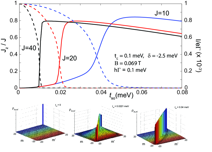
Figure 6: (Color online) Top: Steady-state current, $I$, (solid lines) and nuclear spin polarization, $J_{z}$, (dashed lines) as a function of $t_{\mathrm{so}}$. Three different sizes of large spin are shown, $J=10$ (blue), $J=20$ (red), and $J=40$ (black), corresponding to $N=200$, $400$ and $3800$ nuclear spins respectively. The transition occurs for $t_{\mathrm{so}}>25A/4\sqrt{N}$, where $A$ is the maximum value of the nuclear hyperfine coupling $g=A/N$. Because of the inverse scaling of the transition point, as a function of $N$, these results suggest that a relatively small spin-orbit coupling can suppress the polarization of the nuclear spin. Bottom: matrix elements (in the $m$ basis of the $J_{z}$ operator) of the steady-state reduced density matrix of the nuclear spin, for $J=20$. At the critical point the steady-state contains significant non-zero coherences.

III.2 Nuclear spin polarization

Hysteresis in the current measurement, as one sweeps the external magnetic field through the singlet-triplet level crossing, is a sign of nuclear spin polarization. In vertical dots, large polarizations ($>40\%$) have been achieved. Baugh ; Takahashi ; Kobayashi ; Petta In lateral dots, the polarizations are significantly smaller, perhaps due to either the asymmetry in the dots, and thus in the nuclear hyperfine interaction, or dark states. Gullans However, even for small levels of nuclear spin polarization, large hysteresis has been observed. Further, in several recent studies it has been shown theoretically that if the spin-orbit coupling is above a certain threshold, relative to the nuclear hyperfine coupling, no polarization of the nuclear spin occurs. Rudner10 If it is below that threshold, the nuclear system becomes polarized due to the spin-flip process during the electron transport. At some critical value between these two regimes, long-lived dark states can occur, alongside a topological phase transition.

To investigate this phenomenon in our model we plot, in Fig. 6, both the steady-state current $I$ and the normalized nuclear polarization $J_{z}/J$ as a function of $t_{\mathrm{so}}$ for a given nuclear hyperfine coupling $A=0.1$ meV. We use dot parameters which put us at the singlet-triplet resonance point, and also omit the first term (the Overhauser term) in Eq. (25). We see that for

$$t_{\mathrm{so}}<25A/4\sqrt{N},$$ (29)

the nuclear spin is strongly polarized by the electron transport process, and the current flow is low. Conversely, as

$$t_{\mathrm{so}}>25A/4\sqrt{N},$$ (30)

the spin-orbit mediated transport route becomes dominant, and the nuclear spin is no longer maximally polarized. The transition between these two regimes is consistent with the sharp change observed in the “topological phase transition” Rudner10 . The factor of $25$ arises from the amplitudes $C_{0,2}$ and $C_{1,1}$ of the combined effective singlet state used in that treatment $|S\rangle=C_{0,2}|S(0,2)\rangle+C_{1,1}|S(1,1)\rangle$. Inspection of the bare eigenstates of the electron spin Hamiltonian shows that this factor is, in general,

$$|(C_{1,1}/C_{0,2})|=|(\delta-\sqrt{4t_{c}^{2}+\delta^{2}})/2t_{c}|.$$ (31)

Thus the quantum dot system parameters can in practice also be tuned to sweep the axis of Fig. 6. In the bottom half of Fig. 6 we show the absolute value of the matrix elements (in the basis of the $m\in\{-J,J\}$ eigenstates of $J_{z}$) of the steady-state nuclear spin density matrix for three choices of spin-orbit coupling: zero, at the “critical point” and far above the critical point. One can easily see that at the critical point there are significant non-zero coherences in the nuclear spin state, which may be related to the presence of long-lived “dark states”. Rudner10 Our results indicate that precursors to this “topological phase transition” exist even in the presence of a full transport cycle and noisy environmental effects, akin to the persistence of quantum phase transitions in non-equilibrium systems. Dalla

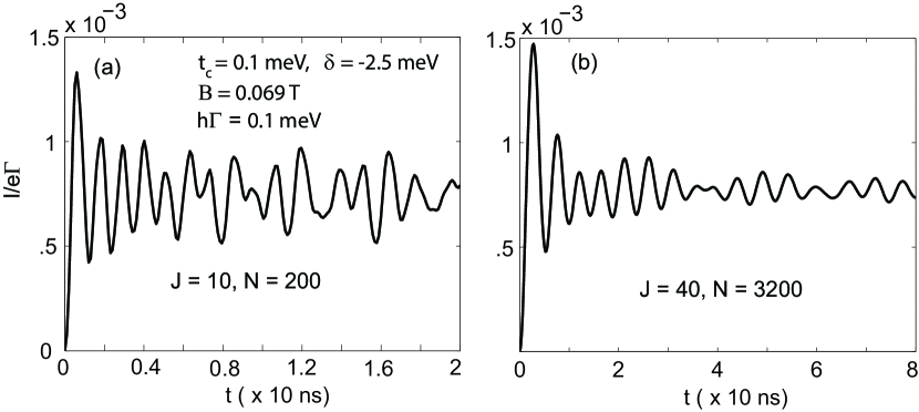
Figure 7: Transient current, $I(t)$, with an initially maximally-mixed nuclear spin state for (a) $J=10$, and (b) $J=40$. The large number of commensurate frequencies around $m=0$ cause the regular oscillations with frequency $A/4\sqrt{N}$, before the onset of quasi-chaotic dynamics.

III.3 Transient dynamics

Some evidence Takahashi ; Reilly indicates that the low dephasing and extremely long relaxation time of the nuclear spins, combined with the fast stochastic electron transport process inducing nuclear polarization, leads to a long time instability phenomenon and fluctuations in the nuclear spin state. Brandes ; Rudner2011 This is typically observed in the long-time beating seen in the current. Takahashi ; Reilly This is almost certainly a semi-classical effect, ono2004 ; Brandes ; Inoshita2004 ; Rudner2011 ; Danon though some evidence suggests that coherence within the nuclear spins can survive for millisecond time scales. Takahashi To gain some insight on what might be observed on shorter time scales, we now examine the transient behaviour of the electron transport induced by the nuclear spin. In the following we entirely neglect the spin-orbit coupling.

We assume that at some initial time $t=0$ the electronic system is prepared in the $|T_{+}\rangle$ state and the nuclear system is in an initially maximally-mixed state

$$\rho(0)=\frac{1}{2J+1}\sum_{m}|m\rangle\langle m|\otimes|T_{+}\rangle\langle T_{+}|.$$ (32)

We then solve the dynamics given by this initial state in the equation of motion. As we will show below, we find that this produces dynamics akin to the Jaynes-Cummings Hamiltonian from quantum optics with an initial thermal (or chaotic) cavity state. Klimov ; Knight This is a well-studied system, with so-called “quasi-chaotic revivals”. In the optical case, studies have shown that one observes an initial sharp peak Knight in the atomic state on a time-scale $t_{p}^{(\mathrm{bosonic})}\approx 2\pi\hbar/\lambda\sqrt{\bar{n}}$, where $\lambda$ is the field-atom coupling in that model, and $\bar{n}$ is the initial thermal occupation of the field given by the Bose-Einstein distribution. This is typically followed by the onset of the so-called “quasi-chaotic” oscillations at a time that scales with the thermal occupation.

In Fig. 7 we show the transient electron current for two sizes of the nuclear spin system. Again we omit the Overhauser term. In the figure, one can see the clear onset of quasi-chaotic beating and a scaling of the onset of this beating with the size of the large spin $J$. Since we are now dealing with an infinite-temperature large spin, the role played by $\bar{n}$ in the optical case is now played by $J$ in the large-spin case. Unlike in the optical case, however, the collapse of an initial peak is not seen here. Instead, there is a transition from large steady oscillations to quasi-chaotic ones.

To understand the presence of the large steady oscillations we can make two observations. Firstly, for low thermal occupation $\bar{n}\ll J$, and large $J$, the Holstein-Primakoff transformation tells us that the dynamics would coincide with that of the bosonic Jaynes-Cummings model, but with renormalized coupling $\lambda\approx A/2\sqrt{2}N$. As $\bar{n}\propto J$, the analogy should break-down. Secondly, the large regular oscillations can be understood by explicit diagonalization of the $H_{\mathrm{hf}}$ Hamiltonian (again omitting the first, Overhauser, term), which gives the following expression for the occupation probability of the $|T_{+}\rangle$ state, assuming that the initial state is $|\psi(0)\rangle=|T_{+}\rangle\otimes\sum_{m=-J}^{J}C_{m}|m\rangle$,

$$|\langle T_{+}|\psi(0)\rangle|^{2}=\sum_{m=-J}^{J}|C_{m}|^{2}\cos^{2}\left(\frac{E_{+}t}{\hbar}\right),$$ (33)

where

$$E_{+}^{(m)}=\frac{A\sqrt{J(J+1)-m(m+1)}}{2\sqrt{2}N}.$$ (34)

In the bosonic case, this is an infinite sum whose frequencies scale as $\sqrt{n+1}$. One can understand the large regular oscillations that occur in the large spin case by considering the contributions to the sum around $m=0$. This region contributes a large number of terms to the sum, with similar frequencies $E_{+}^{(m\approx 0)}/\hbar\approx A/4\hbar\sqrt{N}$, which are commensurate at small times. This gives rise to the frequency of the early-time oscillations in Fig. 7.

The possibility to observe both the early-time oscillations and the quasi-chaotic oscillations in experiment is intriguing. One can consider that as $N$ is increased the period of the oscillations increases. For $N\propto 10^{5}$–$10^{6}$ this can reach the order of 100 micro-seconds. Ultimately, the observation of these oscillations is limited by two effects. First, electron spin dephasing will affect these dynamics. We found that, by including such effects in our model, if these dephasing rates are much larger than the frequency $E_{+}$ the oscillations become damped. However, the oscillations are not strongly affected by dephasing or decoherence in the charge degree of freedom. Secondly, in reality, the width of the distribution of large spins in the thermal ensemble around $\sqrt{N/2}$ will also cause dephasing, and is the primary cause of the electron spin dephasing to begin with. One can consider that large spins in this distribution close to $\sqrt{N/2}$ will contribute “in phase” to the early-time oscillations and those far away will induce additional dephasing. Thus, inevitably the oscillations shown in Fig. 7 will decay if this distribution is broad. Finally, dephasing and rethermalization of the nuclear spin states will also affect the dynamics if these rates become comparable to $E_{+}$.

In addition, the behavior we show in the dynamics of the current occurs on a relatively short time scale and strongly depends on the initial state. We also emphasize that the meaning of this short-time dynamical current we plot in the figures is the following: it is the ensemble average of detecting the current of a single electron entering the reservoir based on a specific initial condition. In other words, in a real experiment, one would have to repeatedly prepare the nuclear-spin and dot system in the same initial state, and measure the resulting single electron transport events to eventually collate the data shown in the figure. Obviously this is experimentally challenging. A more feasible and natural approach would be to detect transient behavior in the high-frequency current-noise spectrum. However, given that such transients are “around the steady state” (a state which may include significant nuclear spin polarization), some of the features which rely on the nuclear spin state being in a maximally-mixed state may become less visible.

In practice, it maybe more feasible to consider a closed system, i.e., disconnected from electronic reservoirs, and measured by, e.g., a charge detector. In this case there will be no dynamical nuclear polarization, which is advantageous for observing the features which rely on the maximally mixed state. Also, at this stage, it is not clear if there is any connection between the oscillations we observe here and those seen in experiments. Even for large $N$ the time scales still differ greatly. Finally, an alternative system to investigate this phenomenon could be quantum dots in carbon nanotubes, or with superconducting qubits/wave guides nature coupled to ensembles of spins in diamond.

IV Conclusions

This work investigated electronic transport in a double quantum dot for weak spin-orbit interaction, namely, when the spin-orbit amplitude is smaller than the interdot coupling. The electrical current was calculated numerically from rate equations. We derived simple approximate expressions for the current as a function of the amplitudes of the one- and two-electron states which participate in the transport cycle. We found that when the SOI is small the current shows a peak at a magnetic field for which the lowest two-electron energy levels anticross, whereas when the SOI is large a dip is formed at zero magnetic field. Numerical calculations showed that in a double dot system with a small hyperfine interaction these characteristics remain valid.

We also considered a model which includes dynamical behavior of the nuclear spin, and investigated the coupled dynamics between electron and nuclear spins. We found that the conflict between the spin-orbit and nuclear hyperfine couplings results in a transition point between no polarization and large polarization of the nuclear spin ensemble. We also considered the transient dynamics, where the nuclear spin ensemble is initially prepared in a highly thermal state. The unique characteristics of the large effective-spin model used to describe the nuclear spin ensemble induces dynamics in the current which depends on the fundamental nuclear hyperfine coupling and the ensemble size.

References

References

- (1) K. Ono, D. G. Austing, Y. Tokura, and S. Tarucha, Science 297, 1313 (2002).
- (2) M. R. Buitelaar, J. Fransson, A. L. Cantone, C. G. Smith, D. Anderson, G. A. C. Jones, A. Ardavan, A. N. Khlobystov, A. A. R. Watt, K. Porfyrakis, and G. A. D. Briggs, Phys. Rev. B 77, 245439 (2008).
- (3) K. Ono and S. Tarucha, Phys. Rev. Lett. 92, 256803 (2004).
- (4) R. M. Abolfath, A. Trojnar, B. Roostaei, T. Brabec, and P. Hawrylak, arxiv:1202.5352.
- (5) A. Pfund, I. Shorubalko, K. Ensslin, and R. Leturcq, Phys. Rev. B 76, 161308(R) (2007).
- (6) S. Nadj-Perge, S. M. Frolov, J. W. W. van Tilburg, J. Danon, Y. V. Nazarov, R. Algra, E. P. A. M. Bakkers, and L. P. Kouwenhoven, Phys. Rev. B 81, 201305 (2010).
- (7) J. Danon and Y. V. Nazarov, Phys. Rev. B 80, 041301(R) (2009).
- (8) F. Romeo and R. Citro, Phys. Rev. B 80, 165311 (2009).
- (9) A. V. Rozhkov, G. Giavaras, Y. P. Bliokh, V. Freilikher, and F. Nori, Phys. Rep. 503, 77 (2011).
- (10) S. J. Chorley, G. Giavaras, J. Wabnig, G. A. C. Jones, C. G. Smith, G. A. D. Briggs, and M. R. Buitelaar, Phys. Rev. Lett. 106, 206801 (2011).
- (11) M. S. Rudner and L. S. Levitov, Phys. Rev. B 82, 155418 (2010).
- (12) O. N. Jouravlev and Y. V. Nazarov, Phys. Rev. Lett. 96, 176804 (2006).
- (13) C. W. Gardiner and P. Zoller, Quantum Noise (Springer, New York, 2000).
- (14) J. R. Petta, A. C. Johnson, J. M. Taylor, E. A. Laird, A. Yacoby, M. D. Lukin, C. M. Marcus, M. P. Hanson, and A. C. Gossard, Science 309, 2180 (2005).
- (15) Numerical results derived from the time evolution of the full density matrix confirm that this is a very good approximation, even when degenerate eigenvalues occur, provided the coupling to the leads is weak. We also ignore cotunneling processes.
- (16) C. Lopez-Monis, C. Emary, G. Kiesslich, G. Platero, and T. Brandes, Phys. Rev. B 85, 045301 (2012).
- (17) T. Inoshita, K. Ono, and S. Tarucha, J. Phys. Soc. Jpn. Supp. A 72, 183 (2002).
- (18) T. Inoshita and S. Tarucha, Physica E 22, 422 (2004).
- (19) I. A. Merkulov, AI. L. Efros, and M. Rosen, Phys. Rev. B. 65, 205309 (2002).
- (20) M. S. Rudner, F. H. L. Koppens, J. A. Folk, L. M. K. Vandersypen, and L. S. Levitov, Phys. Rev. B 84, 075339 (2011).
- (21) W. Yang and R-B Liu, Phys. Rev. B 78, 085315 (2008).
- (22) J. Baugh, Y. Kitamura, K. Ono, and S. Tarucha, Phys. Rev. Lett. 99, 096804 (2007).
- (23) R. Takahashi, K. Kono, S. Tarucha, and K. Ono, Phys. Rev. Lett. 107, 026602 (2011).
- (24) T. Kobayashi, K. Hitachi, S. Sasaki, and K. Muraki, Phys. Rev. Lett. 107, 216802 (2011).
- (25) J. R. Petta, J. M. Taylor, A. C. Johnson, A. Yacoby, M. D. Lukin, C. M. Marcus, M. P. Hanson, and A. C. Gossard, Phys. Rev. Lett. 100, 067601 (2008).
- (26) M. Gullans, J. J. Krich, J. M. Taylor, H. Bluhm, B. I. Halperin, C. M. Marcus, M. Stopa, A. Yacoby, and M. D. Lukin, Phys. Rev. Lett. 104, 226807 (2010).
- (27) E. G. Dalla Torre, E. Demler, T. Giamarchi, and E. Altman, Nature Phys. 6, 806 (2010).
- (28) D. J. Reilly, J. M. Taylor, E. A. Laird, J. R. Petta, C. M. Marcus, M. P. Hanson, and A. C. Gossard, Phys. Rev. Lett. 101, 236803 (2008).
- (29) J. Danon, I. T. Vink, F. H. L. Koppens, K. C. Nowack, L. M. K. Vandersypen, and Y. V. Nazarov, Phys. Rev. Lett. 103, 046601 (2009).
- (30) A. B. Klimov and S. M. Chumakov, Phys. Lett. A 264, 100 (1999).
- (31) P. L. Knight and P. M. Radmore, Phys. Lett. 90A, 342 (1982).
- (32) J. Q. You and F. Nori, Nature 474, 589 (2011).