Incidence coloring game and arboricity of graphs

Abstract

An incidence of a graph $G$ is a pair $(v,e)$ where $v$ is a vertex of $G$ and $e$ an edge incident to $v$. Two incidences $(v,e)$ and $(w,f)$ are adjacent whenever $v=w$, or $e=f$, or $vw=e$ or $f$. The incidence coloring game [S.D. Andres, The incidence game chromatic number, Discrete Appl. Math. 157 (2009), 1980–1987] is a variation of the ordinary coloring game where the two players, Alice and Bob, alternately color the incidences of a graph, using a given number of colors, in such a way that adjacent incidences get distinct colors. If the whole graph is colored then Alice wins the game otherwise Bob wins the game. The incidence game chromatic number $i_{g}(G)$ of a graph $G$ is the minimum number of colors for which Alice has a winning strategy when playing the incidence coloring game on $G$.

Andres proved that $i_{g}(G)\leq 2\Delta(G)+4k-2$ for every $k$-degenerate graph $G$. We show in this paper that $i_{g}(G)\leq\lfloor\frac{3\Delta(G)-a(G)}{2}\rfloor+8a(G)-2$ for every graph $G$, where $a(G)$ stands for the arboricity of $G$, thus improving the bound given by Andres since $a(G)\leq k$ for every $k$-degenerate graph $G$. Since there exists graphs with $i_{g}(G)\geq\lceil\frac{3\Delta(G)}{2}\rceil$, the multiplicative constant of our bound is best possible.

Keywords: Arboricity; Incidence coloring; Incidence coloring game; Incidence game chromatic number.

1 Introduction

All the graphs we consider are finite and undirected. For a graph $G$, we denote by $V(G)$, $E(G)$ and $\Delta(G)$ its vertex set, edge set and maximum degree, respectively. Recall that a graph is $k$-denegerate if all of its subgraphs have minimum degree at most $k$.

The graph coloring game on a graph $G$ is a two-player game introduced by Brams [8] and rediscovered ten years after by Bodlaender [3]. Given a set of $k$ colors, Alice and Bob take turns coloring properly an uncolored vertex of $G$, Alice having the first move. Alice wins the game if all the vertices of $G$ are eventually colored, while Bob wins the game whenever, at some step of the game, all the colors appear in the neighborhood of some uncolored vertex. The game chromatic number $\chi_{g}(G)$ of $G$ is then the smallest $k$ for which Alice has a winning strategy when playing the graph coloring game on $G$ with $k$ colors.

The problem of determining the game chromatic number of planar graphs has attracted great interest in recent years. Kierstead and Trotter proved in 1994 that every planar graph has game chromatic number at most 33 [10]. This bound was decreased to 30 by Dinski and Zhu [5], then to 19 by Zhu [15], to 18 by Kierstead [9] and to 17, again by Zhu [16], in 2008. Some other classes of graphs have also been considered (see [2] for a comprehensive survey).

An incidence of a graph $G$ is a pair $(v,e)$ where $v$ is a vertex of $G$ and $e$ an edge incident to $v$. We denote by $I(G)$ the set of incidences of $G$. Two incidences $(v,e)$ and $(w,f)$ are adjacent if either (1) $v=w$, (2) $e=f$ or (3) $vw=e$ or $f$. An incidence coloring of $G$ is a coloring of its incidences in such a way that adjacent incidences get distinct colors. The smallest number of colors required for an incidence coloring of $G$ is the incidence chromatic number of $G$, denoted by $\chi_{i}(G)$. Let $G$ be a graph and $S(G)$ be the full subdivision of $G$, obtained from $G$ by subdividing every edge of $G$ (that is, by replacing each edge $uv$ by a path $ux_{uv}v$, where $x_{uv}$ is a new vertex of degree 2). It is then easy to observe that every incidence coloring of $G$ corresponds to a strong edge coloring of $S(G)$, that is a proper edge coloring of $S(G)$ such that every two edges with the same color are at distance at least 3 from each other [4]. Observe also that any incidence coloring of $G$ is nothing but a distance-two coloring of the line-graph of $G$ [13], that is a proper vertex coloring of the line-graph of $G$ such that any two vertices at distance two from each other get distinct colors.

Incidence colorings have been introduced by Brualdi and Massey [4] in 1993. Upper bounds on the incidence chromatic number have been proven for various classes of graphs such as $k$-degenerate graphs and planar graphs [6, 7], graphs with maximum degree three [12], and exact values are known for instance for forests [4], $K_{4}$-minor-free graphs [7], or Halin graphs with maximum degree at least 5 [14] (see [13] for an on-line survey).

In [1], Andres introduced the incidence coloring game, as the incidence version of the graph coloring game, each player, on his turn, coloring an uncolored incidence of $G$ in a proper way. The incidence game chromatic number $i_{g}(G)$ of a graph $G$ is then defined as the smallest $k$ for which Alice has a winning strategy when playing the incidence coloring game on $G$ with $k$ colors. Upper bounds on the incidence game chromatic number have been proven for $k$-degenerate graphs [1] and exact values are known for cycles, stars [1], paths and wheels [11].

Andres observed that the inequalities $\lceil\frac{3}{2}\Delta(G)\rceil\leq i_{g}(F)\leq 3\Delta(G)-1$ hold for every graph $G$ [1]. For $k$-degenerate graphs, he proved the following:

Theorem 1 (Andres, [1]).

Let $G$ be a $k$-degenerated graph. Then we have:

1. $i_{g}(G)\leq 2\Delta(G)+4k-2$,

2. $i_{g}(G)\leq 2\Delta(G)+3k-1$ if $\Delta(G)\geq 5k-1$,

3. $i_{g}(G)\leq\Delta(G)+8k-2$ if $\Delta(G)\leq 5k-1$.

Since forests, outerplanar graphs and planar graphs are respectively 1-, 2- and 5-degenerate, we get that $i_{g}(G)\leq 2\Delta(G)+2$, $i_{g}(G)\leq 2\Delta(G)+6$ and $i_{g}(G)\leq 2\Delta(G)+18$ whenever $G$ is a forest, an outerplanar graph or a planar graph, respectively.

Recall that the arboricity $a(G)$ of a graph $G$ is the minimum number of forests into which its set of edges can be partitioned. In this paper, we will prove the following:

Theorem 2.

For every graph $G$, $i_{g}(G)\leq\lfloor\frac{3\Delta(G)-a(G)}{2}\rfloor+8a(G)-1$.

Recall that $i_{g}(G)\geq 3\Delta(G)/2$ for every graph $G$ so that the difference between the upper and the lower bound on $i_{c}(G)$ only depends on the arboricity of $G$.

It is not difficult to observe that $a(G)\leq k$ whenever $G$ is a $k$-degenerate graph. Hence we get the following corollary, which improves Andres’ Theorem and answers in the negative a question posed in [1]:

Corollary 3.

If $G$ is a $k$-degenerate graph, then $i_{g}(G)\leq\lfloor\frac{3\Delta(G)-k}{2}\rfloor+8k-1$

Since outerplanar graphs and planar graphs have arboricity at most 2 and 3, respectively, we get as a corollary of Theorem 2 the following:

Corollary 4.

1. $i_{g}(G)\leq\lceil\frac{3\Delta(G)}{2}\rceil+6$ for every forest $G$,

2. $i_{g}(G)\leq\lfloor\frac{3\Delta(G)}{2}\rfloor+14$ for every outerplanar graph $G$,

3. $i_{g}(G)\leq\lceil\frac{3\Delta(G)}{2}\rceil+21$ for every planar graph $G$.

We detail Alice’s strategy in Section 2 and prove Theorem 2 in Section 3.

2 Alice’s Strategy

We will give a strategy for Alice which allows her to win the incidence coloring game on a graph $G$ with arboricity $a(G)$ whenever the number of available colors is at least $\lfloor\frac{3}{2}\Delta(G)\rfloor+8a(G)-1$. This strategy will use the concept of activation strategy [2], often used in the context of the ordinary graph coloring game.

Let $G$ be a graph with arboricity $a(G)=a$. We partition the edges of $G$ into $a$ forests $F_{1}$, …, $F_{a}$, each forest containing a certain number of trees. For each tree $T$, we choose an arbitrary vertex of $T$, say $r_{T}$, to be the root of $T$.

Notation.

Each edge with endvertices $u$ and $v$ in a tree $T$ will be denoted by $uv$ if $dist_{T}(u,r_{T})<dist_{T}(v,r_{T})$, and by $vu$ if $dist_{T}(v,r_{T})<dist_{T}(u,r_{T})$, where $dist_{T}$ stands for the distance within the tree $T$ (in other words, we define an orientation of the graph $G$ in such a way that all the edges of a tree $T$ are oriented from the root towards the leaves).

We now give some notation and definitions we will use in the sequel (these definitions are illustrated in Figure 1).

• For every edge $uv$ belonging to some tree $T$, we say the incidence $(u,uv)$ is a top incidence whereas the incidence $(v,uv)$ is a down incidence. We then let $t(uv)=t(v,vu)=(u,uv)$ and $d(uv)=d(u,uv)=(v,uv)$.
  Note that each vertex in a forest $F_{i}$ is incident to at most one down incidence belonging to $F_{i}$, so that each vertex in $G$ is incident to at most $a$ down incidences.

• For every incidence $i$ belonging to some edge $uv\in E(G)$, let $tF(i)=\{t(wu),\ wu\in E(G)\}$ be the set of top-fathers of $i$, $dF(i)=\{d(wu),\ wu\in E(G)\}$ be the set of down-fathers of $i$ and $F(i)=tF(i)\cup dF(i)$ be the set of fathers of $i$.
  Note that each incidence has at most $a$ top-fathers and at most $a$ down-fathers.

• For every incidence $i$ belonging to some edge $uv\in E(G)$, let $tS(i)=\{t(vw),\ vw\in E(G)\}$ be the set of top-sons of $i$, $dS(i)=\{d(vw),\ vw\in E(G)\}$ be the set of down-sons of $i$ and $S(i)=tS(i)\cup dS(i)$ be the set of sons of $i$.
  Note that each incidence has at most $\Delta(G)-1$ top-sons and at most $\Delta(G)-1$ down-sons.

• For every incidence $i$ belonging to some edge $uv\in E(G)$, let $tB(i)=\{t(uw),\ uw\in E(G)\}-\{i\}$ be the set of top-brothers of $i$, $dB(i)=\{d(uw),\ uw\in E(G)\}-\{i\}$ be the set of down-brothers of $i$ and $B(i)=tB(i)\cup dB(i)$ be the set of brothers of $i$.
  Note that each top incidence $i$ has at most $\Delta(G)-|tF(i)|-1$ top-brothers and $\Delta(G)-|tF(i)|$ down-brothers while each down incidence $j$ has at most $\Delta(G)-|tF(j)|$ top-brothers and $\Delta(G)-|tF(j)|-1$ down-brothers.
  Note also that any two brother incidences have exactly the same set of fathers.

• Finally, for every incidence $i$ belonging to some edge $uv\in E(G)$, let $tU(i)=\{t(wv),\ wv\in E(G)\}$ be the set of top-uncles of $i$, $dU(i)=\{d(wv),\ wv\in E(G)\}$ be the set of down-uncles of $i$ and $U(i)=tU(i)\cup dU(i)$ be the set of uncles of $i$ (the term ”uncle” is not metaphorically correct since the uncle of an incidence $i$ is another father of the sons of $i$ rather than a brother of a father of $i$).
  Note that each incidence has at most $a-1$ top-uncles and at most $a-1$ down-uncles. Moreover, we have $|dU(i)|+|tS(i)|\leq\Delta(G)-1$ for every incidence $i\in I(G)$.

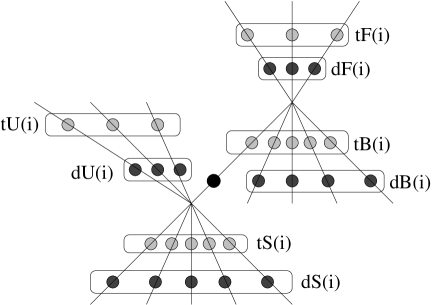
Figure 1: Incidences surrounding the incidence $i$.

Figure 1 illustrates the above defined sets of incidences. Each edge is drawn in such a way that its top incidence is located above its down incidence. Incidence $i$ is drawn as a white box, top incidences are drawn as grey boxes and down incidences (except $i$) are drawn as black boxes.

We now turn to the description of Alice’s strategy. For each set $I$ of incidences, we will denote by $I_{c}$ the set of colored incidences of $I$. We will use an activation strategy. During the game, each uncolored incidence may be either active (if Alice activated it) or inactive. When the game starts, every incidence is inactive. When an active incidence is colored, it is no longer considered as active. In our strategy, it is sometimes possible that we say Alice activates an incidence that is already colored, but still considered as inactive. For each set $I$ of incidences, we will denote by $I_{a}$ the set of active incidences of $I$ ($I_{a}$ and $I_{c}$ are therefore disjoint for every set of incidences $I$).

We denote by $\Phi$ the set of colors used for the game, by $\phi(i)$ the color of an incidence $i$ and, for each set $I$ of incidences, we let $\phi(I)=\bigcup_{i\in I}\phi(i)$. As shown by Figure 1, the set of forbidden colors for an uncolored incidence $i$ is given by:

• $\phi(F(i)\cup B(i)\cup tS(i)\cup dU(i))$ if $i$ is a top incidence,

• $\phi(dF(i)\cup tB(i)\cup S(i)\cup U(i))$ if $i$ is a down incidence.

Our objective is therefore to bound the cardinality of these sets. We now define the subset $I_{n}$ of neutral incidences of $I(G)$, which contains all the incidences $j$ such that:

1. $j$ is not colored,

2. all the incidences of $F(j)$ are colored.

We also describe what we call a neutral move for Alice, that is a move Alice makes only if there is no neutral incidence and no activated incidence in the game. Let $i_{0}$ be any uncolored incidence of $I(G)$. Since there is no neutral incidence, either there is an uncolored incidence $i_{1}$ in $dF(i_{0})$, or all the incidences of $dF(i_{0})$ are colored and there is an uncolored incidence $i_{1}$ in $tF(i_{0})$. We define in the same way incidences $i_{2}$ from $i_{1}$, $i_{3}$ from $i_{2}$, and so on, until we reach an incidence that has been already encountered. We then have $i_{k}=i_{\ell}$ for some integers $k$ and $\ell$, with $k\leq\ell$. The neutral move of Alice then consists in activating all the incidences within the loop and coloring any one of them.

Alice’s strategy uses four rules. The first three rules, (R1), (R2) and (R3) below, determine which incidence Alice colors at each move. The fourth rule explains which color will be used by Alice when she colors an incidence.

1. On her first move,

   • If there is a neutral incidence (i.e., in this case, an incidence without fathers), then Alice colors it.

   • Otherwise, Alice makes a neutral move.

2. If Bob, in his turn, colors a down incidence $i$ with no uncolored incidence in $dF(i)$, then

   1. If there are uncolored incidences in $dB(i)$, then Alice colors one of them,

   2. Otherwise,

      • If there is a neutral incidence or an activated incidence in $I(G)$, then Alice colors it,

      • If not, Otherwise, Alice makes a neutral move.

3. If Bob colors another incidence, then Alice climbs it. Climbing an incidence $i$ is a recursive procedure, described as follows:

   1. If $i$ is active, then Alice colors $i$.

   2. Otherwise, Alice activates $i$ and:

      • If there are uncolored incidences in $dF(i)$, then Alice climbs one of them.

      • If all the incidences of $dF(i)$ are colored, and if there are uncolored incidences in $tF(i)$, then Alice climbs one of them.

      • If all the incidences of $F(i)$ are colored, then:

        • if there is a neutral incidence or an activated incidence in $I(G)$, then Alice colors it,

        • otherwise, Alice makes a neutral move.

4. When Alice has to color an incidence $i$, she proceeds as follows: if $i$ is a down incidence with $|\phi(dB(i))|\geq 4a-1$, she uses any available color in $\phi(dB(i))$; in all other cases, she chooses any available color.

Observe that, in a neutral move, all the incidences $i_{k},i_{k+1},\dots,i_{\ell}$ form a loop where each incidence can be reached by climbing the previous one. We consider that, when Alice does a neutral move, all the incidences are climbed at least one.

Then we have:

Observation 5.

When an inactive incidence is climbed, it is activated. When an active incidence is climbed, it is colored. Therefore, every incidence is climbed at most twice.

Observation 6.

Alice only colors neutral incidences or active incidences (typically, incidences colored by Rule (R2.2.1) are neutral incidences), except when she makes a neutral move.

3 Proof ot Theorem 2

We now prove a series of lemmas from which the proof of Theorem 2 will follow.

Lemma 7.

When Alice or Bob colors a down incidence $i$, we have

$$|S_{c}(i)|+|U_{c}(i)|\leq 4a-2.$$

When Alice or Bob colors a top incidence $i$, we have

$$|tS_{c}(i)|+|dU_{c}(i)|\leq 5a-1.$$

Proof.

Let first $i$ be a down incidence that has just been colored by Bob or Alice. If $|S_{c}(i)|=0$, then $|S_{c}(i)|+|U_{c}(i)|=|U_{c}(i)|\leq|U(i)|\leq 2a-2$. Otherwise, let $j$ be an incidence from $S(i)$ which was colored before $i$.

• If $j$ was colored by Bob, then Alice has climbed $i$ or some other incidence from $dU(i)$ in her next move by Rule (R2.1).

• If $j$ was colored by Alice, then

  • either $j$ was an active incidence and, when $j$ has been activated, Alice has climbed either $d(i)$, or $i$, or some other incidence from $U(i)$,

  • or Alice has made a neutral move and, in the same move, has activated either $d(i)$, or $i$, or some other incidence from $U(i)$.

By Observation 5 every incidence is climbed at most twice, and thus $|S_{c}(i)|\leq 2\times(|dU(i)|+1)$. Since $|dU(i)|\leq a-1$, we have $|S_{c}(i)|\leq 2a$. Moreover, since $|U_{c}(i)|\leq|U(i)|\leq 2a-2$, we get $|S_{c}(i)|+|U_{c}(i)|\leq 4a-2$ as required.

Let now $i$ be a top incidence that has just been colored by Bob or Alice. If $|tS_{c}(i)|=0$, then $|tS_{c}(i)|+|dU_{c}(i)|=|dU_{c}(i)|\leq|dU(i)|\leq a-1$. Otherwise, let $j$ be an incidence from $tS(i)$ which was colored before $i$.

• If $j$ was colored by Bob then, in her next move, Alice either has climbed $d(i)$ or some other incidence from $dU(i)$ by Rule (R2.1), or $i$ or some other incidence from $tU(i)$ by Rule (R2.3).

• If $j$ was colored by Alice, then

  • either $j$ was an active incidence and, when $j$ has been activated, Alice has climbed either $d(i)$, or $i$, or some other incidence from $U(i)$,

  • or Alice has made a neutral move and, in the same move, has activated either $d(i)$, or $i$, or some other incidence from $U(i)$.

By Observation 5 every incidence is climbed at most twice, and thus $|tS_{c}(i)|\leq 2\times(|U(i)|+2)$. Since $|U(i)|\leq 2a-2$, we have $|tS_{c}(i)|\leq 4a$. Moreover, since $|dU_{c}(i)|\leq|dU(i)|\leq a-1$, we get $|tS_{c}(i)|+|dU_{c}(i)|\leq 5a-1$ as required. ∎

Lemma 8.

Whenever Alice or Bob colors a down incidence $i$, there is always an available color for $i$ if $|\Phi|\geq\Delta(G)+5a-2$. Moreover, if $|\phi(dB(i))|\geq 4a-1$, then there is always an available color in $\phi(dB(i))$ for coloring $i$.

Proof.

When Alice or Bob colors a down incidence $i$, the forbidden colors for $i$ are the colors of $tB(i)$, $dF(i)$, $S(i)$ and $U(i)$.

Observe that $|dF(i)|+|tB(i)|\leq\Delta(G)-1$ for each down incidence $i$, so $|\phi(dF(i))|+|\phi(tB(i))|\leq\Delta(G)-1$.

Now, since $|\phi(S(i))|+|\phi(U(i))|\leq|S_{c}(i)|+|U_{c}(i)|\leq 4a-2$ by Lemma 7, we get that there are at most $\Delta(G)+5a-3$ forbidden colors, and therefore an available color for $i$ whenever $|\Phi|\geq\Delta(G)+5a-2$.

Moreover, since the colors of $\phi(dF(i))$ and $\phi(tB(i))$ are all distinct from those of $\phi(dB(i))$, there are at most $|S_{c}(i)|+|U_{c}(i)|\leq 4a-2$ colors of $\phi(dB(i))$ that are forbidden for $i$, and therefore an available color for $i$ whenever $|\phi(dB(i))|\geq 4a-1$. ∎

Lemma 9.

For every incidence $i$, $|\phi(dB(i))|\leq\lfloor\frac{|dB(i)|}{2}\rfloor+2a$.

Proof.

For every incidence $i$, as soon as $|\phi(dB(i))|=4a-1$, there are at least $4a-1$ colored incidences in $dB(i)$. If $dF(i)$ is not empty, then every incidence in $dF(i)$ has thus at least $4a-1$ colored sons so that, by Lemma 7, every such incidence is already colored. During the rest of the game, each time Bob will color an incidence of $dB(i)$, if there are still some uncolored incidences in $dB(i)$, then Alice will answer by coloring one of them by Rule (R2.2.1). Hence, Bob will color at most $\lceil\frac{|dB(i)-(4a-1)|}{2}\rceil$ of these incidences. Since, by Rule (R3), Alice uses colors already in $\phi(dB(i))$ for the incidences she colors, we get $|\phi(dB(i))|\leq 4a-1+\lceil\frac{|dB(i)-(4a-1)|}{2}\rceil\leq\lfloor\frac{|dB(i)|}{2}\rfloor+2a$ as required. ∎

Lemma 10.

When Alice or Bob colors a top incidence $i$, there is always an available color for $i$ whenever $|\Phi|\geq\lfloor\frac{3\Delta(G)-a}{2}\rfloor+8a-1$.

Proof.

Let $i$ be any uncolored top incidence. The forbidden colors for $i$ are the colors of $tF(i)$, $dF(i)$, $tB(i)$, $dB(i)$, $dU(i)$ and $tS(i)$. We have:

• $|\phi(tF(i))|+|\phi(tB(i))|\leq|tF(i)|+|tB(i)|\leq\Delta(G)-1$,

• $|\phi(dF(i))|\leq|dF(i)|\leq a$ and, by Lemma 9, $|\phi(dB(i))|\leq\lfloor\frac{|dB(i)|}{2}\rfloor+2a$; since $|dF(i)|+|dB(i)|\leq\Delta(G)$, we get

  $|\phi(dF(i))|+|\phi(dB(i))|$	$\leq$	$|dF(i)|+\lfloor\frac{\Delta(G)-|dF(i)|}{2}\rfloor+2a$
  	$=$	$\lceil\frac{3|dF(i)|}{2}\rceil+\lfloor\frac{\Delta(G)}{2}\rfloor+2a$
  	$\leq$	$\lceil\frac{3a}{2}\rceil+\lfloor\frac{\Delta(G)}{2}\rfloor+2a$
  	$=$	$\lfloor\frac{\Delta(G)-a}{2}\rfloor+3a$,

• $|\phi(tS(i))|+|\phi(dU(i))|\leq 5a-1$ by Lemma 7.

So there are at most $\lfloor\frac{3\Delta(G)-a}{2}\rfloor+8a-2$ forbidden colors for $i$ and the result follows. ∎

Lemma 10 shows that, when Alice applies the strategy above described, every top incidence can be colored, provided $|\Phi|\geq\lfloor\frac{3\Delta(G)-a}{2}\rfloor+8a-1$. Lemma 8 shows that this is also the case for down incidences, which proves Theorem 2.

References

- [1] S.D. Andres. The incidence game chromatic number. Discrete Appl. Math., 157:1980–1987, 2009.
- [2] T. Bartnicki, J. Grytczuk, H. A. Kierstead, and X. Zhu. The map coloring game. Amer. Math., Monthly, November, 2007, 2007.
- [3] H.L. Bodlaender. On the complexity of some coloring games. Inter. J. of Found. Computer Science, 2:133–147, 1991.
- [4] R.A. Brualdi and J.J.Q. Massey. Incidence and strong edge colorings of graphs. Discrete Math., 122:51–58, 1993.
- [5] T. Dinski and X. Zhu. Game chromatic number of graphs. Discrete Maths, 196:109–115, 1999.
- [6] M. Hosseini Dolama and E. Sopena. On the maximum average degree and the incidence chromatic number of a graph. Discrete Math. and Theoret. Comput. Sci., 7(1):203–216, 2005.
- [7] M. Hosseini Dolama, E. Sopena, and X. Zhu. Incidence coloring of k-degenerated graphs. Discrete Math., 283:121–128, 2004.
- [8] M. Gardner. Mathematical game. Scientific American, 23, 1981.
- [9] H.A. Kierstead. A simple competitive graph coloring algorithm. J. Combin. Theory Ser. B, 78(1):57–68, 2000.
- [10] H.A. Kierstead and W.T. Trotter. Planar graph coloring with an uncooperative partner. J. Graph Theory, 18:569–584, 1994.
- [11] J.Y. Kim. The incidence game chromatic number of paths and subgraphs of wheels. Discrete Appl. Math., 159:683–694, 2011.
- [12] M. Maydansky. The incidence coloring conjecture for graphs of maximum degree three. Discrete Math., 292:131–141, 2005.
- [13] E. Sopena. www.labri.fr/perso/sopena/TheIncidenceColoringPage.
- [14] S.D. Wang, D.L. Chen, and S.C. Pang. The incidence coloring number of Halin graphs and outerplanar graphs. Discrete Math., 256:397–405, 2002.
- [15] X. Zhu. The game coloring number of planar graphs. J. Combin. Theory Ser. B, 75(2):245–258, 1999.
- [16] X. Zhu. Refined activation strategy for the marking game. J. Combin. Theory Ser. B, 98(1):1–18, 2008.