A GCV based Arnoldi-Tikhonov regularization method

Abstract

For the solution of linear discrete ill-posed problems, in this paper we consider the Arnoldi-Tikhonov method coupled with the Generalized Cross Validation for the computation of the regularization parameter at each iteration. We study the convergence behavior of the Arnoldi method and its properties for the approximation of the (generalized) singular values, under the hypothesis that Picard condition is satisfied. Numerical experiments on classical test problems and on image restoration are presented.

Key words. Linear discrete ill-posed problem. Tikhonov regularization. Arnoldi algorithm. Generalized Cross Validation.

1 Introduction

In this paper we consider discrete ill-posed problems,

$$Ax=b,\quad A\in\mathbb{R}^{N\times N},\text{ }b\in\mathbb{R}^{N},$$ (1)

in which the right-hand side $b$ is assumed to be affected by noise, caused by measurement or discretization errors. These systems typically arise from the discretization of linear ill-posed problem, such as Fredholm integral equations of the first kind with compact kernel (see e.g. [14, Chapter 1] for a background). A common property of these kind of problems, is that the singular values of the kernel rapidly decay and cluster near zero. In this situation, provided that the discretization which leads to (1) is consistent with the continuous problem, this property is inherited by the matrix $A$.

Because of the ill conditioning of $A$ and the presence of noise in $b$, some sort of regularization is generally employed for solving this kind of problems. In this framework, a popular and well established regularization technique is the Tikhonov method, which consists in solving the minimization problem

$$\min_{x\in\mathbb{R}^{N}}\left\{\|Ax-b\|^{2}+\lambda^{2}\|Lx\|^{2}\right\},$$ (2)

where $\lambda>0$ is the regularization parameter and $L\in\mathbb{R}^{P\times N}$ is the regularization matrix (see e.g. [13] and [14] for a background). We denote the solution of (2) by $x_{\lambda}$. For a discussion about the choice of $L$ we may quote here the recent work [5] and the references therein. As well known, the choice of the parameter $\lambda$ is crucial in this setting, since it defines the amount of regularization one wants to impose. Many techniques have been developed to determine a suitable value for the regularizing parameter and we can refer to the recent papers [27, 2, 10, 19] for the state of the art, comparison and discussions. We remark that in (2) and throughout the paper, the norm used is always the Euclidean norm.

Assuming that $b=\overline{b}+e$, where $\overline{b}$ represents the unknown error-free right-hand side, in this paper we assume that no information is available on the error $e$. In such a situation, the most popular and established techniques for the definition of $\lambda$ in (2), as for instance the L-curve criterion and the Generalized Cross Validation (GCV), typically requires the computation of the GSVD of the matrix pair $(A,L)$. Of course this decomposition may represents a serious computational drawback for large-scale problems, such as the image deblurring. In order to overcome this problem, Krylov projection methods such as the ones based on the Lanczos bidiagonalization [1, 11, 17, 18] and the Arnoldi algorithm [3, 21] are generally used. Pure iterative methods such as the GMRES or the LSQR, eventually implemented in a hybrid fashion ([14, § 6.6]) can also be considered in this framework.

In this paper we analyze the Arnoldi method for the solution of (2) (the so called Arnoldi-Tikhonov method, introduced in [3]), coupled with the GCV as parameter choice rule. Similarly to what made in [4] for the Lanczos bidiagonalization process, we show that the resulting algorithm can be fruitfully used for large-scale regularization. Being based on the orthogonal projection of the matrix $A$ onto the Krylov subspaces $\mathcal{K}_{m}(A,b)=\mathrm{span}\{b,Ab,\dots,A^{m-1}b\}$, we shall observe that for discrete ill-posed problems, the Arnoldi algorithm is particularly efficient for the approximation of the GCV curve, after a very few number of iterations.

Indeed, under the hypothesis that Picard condition is satisfied [12], we provide some theoretical results about the convergence of the Arnoldi-Tikhonov methods and its properties for the approximation of the singular values of$\ A$. These properties allow us to consider approximation of the GCV curve which can be obtained working in small dimension (similarly to what made in [3]  where a ”projected” L-curve criterion is used). The GCV curve approximation leads to the definition of a sequence of regularization parameters (one for each step of the algorithm), which are fairly good approximation of the regularization parameter arising from the exact SVD (or GSVD).

The paper is organized as follows. In Section 2 we present a brief outline about the Arnoldi-Tikhonov method for the iterative solution of (2). In Section 3 and 4 we provide some theoretical results concerning the convergence of the Arnoldi algorithm and the SVD (GSVD) approximation. In Section 5 we explain the use the AT method with the GCV criterion. Some numerical experiments are presented in Section 6 and 7.

2 The Arnoldi-Tikhonov method

Denoting by $\mathcal{K}_{m}(A,b)=\mathrm{span}\{b,Ab,\dots,A^{m-1}b\}$ the Krylov subspaces generated by $A$ and the vector $b$, the Arnoldi algorithm computes an orthonormal basis $\left\{w_{1},...,w_{m}\right\}$ of $\mathcal{K}_{m}(A,b)$. Setting $W_{m}=[w_{1},...,w_{m}]\in\mathbb{R}^{N\times m}$, the algorithm can be written in matrix form as

$$AW_{m}=W_{m}H_{m}+h_{m+1,m}w_{m+1}e_{m}^{T},$$ (3)

where $H_{m}=(h_{i,j})\in\mathbb{R}^{m\times m}$ is an upper Hessenberg matrix which represents the orthogonal projection of $A$ onto $\mathcal{K}_{m}(A,b)$, and $e_{m}=(0,...,0,1)^{T}\in\mathbb{R}^{m}$. Equivalently, the relation (3) can be written as

$$AW_{m}=W_{m+1}\overline{H}_{m},$$ (4)

where

$$\overline{H}_{m}=\left[\begin{array}[]{c}H_{m}\\ h_{m+1,m}e_{m}^{T}\end{array}\right]\in\mathbb{R}^{(m+1)\times m}.$$ (5)

In exact arithmetics the Arnoldi process terminates whenever $h_{m+1,m}=0$, which means that $\mathcal{K}_{m+1}(A,b)=\mathcal{K}_{m}(A,b)$.

If we consider the constrained minimization

$$\min_{x\in\mathcal{K}_{m}(A,b)}\left\{\|Ax-b\|^{2}+\lambda^{2}\|Lx\|^{2}\right\},$$ (6)

writing $x=W_{m}y_{m}$, $y_{m}\in\mathbb{R}^{m}$, and using (4), we obtain

$$\min_{y_{m}\in\mathbb{R}^{m}}\left\{\left\|\overline{H}_{m}y_{m}-\left\|b\right\|e_{1}\right\|^{2}+\lambda^{2}\left\|LW_{m}y_{m}\right\|^{2}\right\},$$ (7)

which is known as the Arnoldi-Tikhonov (AT) method. Dealing with Krylov type solvers, one generally hopes that a good approximation of the exact solution can be achieved for $m\ll N$, which, in other words, means that the spectral properties of the matrix $A$ are rapidly simulated by the ones of $\overline{H}_{m}$. This method has been introduced in [3] in the case of $L=I_{N}$ (where $I_{N}$ is the identity matrix of order $N$, so that $\left\|LW_{m}y_{m}\right\|=\left\|y_{m}\right\|$) with the basic aim of reducing the dimension of the original problem and to avoid the matrix-vector multiplication with $A^{T}$ used by Lanczos type schemes (see [1, 11] and the references therein).

It is worth noting that (7) can also be interpreted as an hybrid method. Indeed, the minimization (7) with $L=I_{N}$ is equivalent to the inner regularization of the GMRES [18]. We remark however, that for $L\neq I_{N}$, the philosophy is completely different, since (7) represents the projection of a regularization, while the hybrid approach aims to regularize the projected problem. As we shall see, this difference can be appreciated more clearly whenever a parameter choice rule for $\lambda$ is adopted.

As well known, in many applications the use of a suitable regularization operator $L\neq I_{N}$, may substantially improve the quality of the approximate solution with respect to the choice of $L=I_{N}$. Anyway, we need to observe that with a general $L\in\mathbb{R}^{P\times N}$, the minimization (7) is equivalent to

$$\min_{y_{m}\in\mathbb{R}^{m}}\left\|\left(\begin{array}[]{c}\overline{H}_{m}\\ \lambda LW_{m}\end{array}\right)y_{m}-\left(\begin{array}[]{c}\left\|b\right\|e_{1}\\ 0\end{array}\right)\right\|^{2},$$ (8)

so that, for $P\approx N$, the dimension of (8) inherits the dimension of the original problem. Computationally, the situation can be efficiently faced by means of the ”skinny” QR factorization. Anyway, assuming that $P\leq N$, in order to work with reduced dimension problems, we add $N-P$ zero rows to $L$ (which does not alter (6)) and consider the orthogonal projection of $L$ onto $\mathcal{K}_{m}(A,b)$, that is,

$$L_{m}:=W_{m}^{T}LW_{m}\in\mathbb{R}^{m\times m}.$$ (9)

This modification leads to the reduced minimization

$$\min_{y_{m}\in\mathbb{R}^{m}}\left\{\left\|\overline{H}_{m}y_{m}-\left\|b\right\|e_{1}\right\|^{2}+\lambda^{2}\left\|L_{m}y_{m}\right\|^{2}\right\}$$

$$= \min_{x\in\mathcal{K}_{m}(A,b)}\left\{\|Ax-b\|^{2}+\lambda^{2}\|W_{m}^{T}Lx\|^{2}\right\},$$

which is not equivalent to (6) anymore. Anyway, the use of $L_{m}$ appears natural in this framework, and it is also justified by the fact that

$$\left\|W_{m}^{T}Lx\right\|\leq\|Lx\|,$$

since $\left\|W_{m}^{T}Lx\right\|=\left\|W_{m}W_{m}^{T}Lx\right\|$ and $\left\|W_{m}W_{m}^{T}\right\|=1$, being $W_{m}W_{m}^{T}$ an orthogonal projection. We observe moreover that $L_{m}$ would be the regularization operator of the projection of a Franklin type regularization [6]

$$\left(A+\lambda L\right)x=b.$$

3 Convergence analysis for discrete ill-posed problems

In what follows we denote by $A=U\Sigma V^{T}\in\mathbb{R}^{N\times N}$ the SVD of $A$ where $\Sigma=diag(\sigma_{1},...,\sigma_{N})$, and by $A_{m}:=$ $U_{m}\Sigma_{m}V_{m}^{T}$ the truncated SVD. We remember that the matrix $\Delta_{m}:=A-A_{m}$ is such that $\left\|\Delta_{m}\right\|=\sigma_{m+1}$.

An important property of the methods based on orthogonal projections such as the Arnoldi algorithm, is the fast theoretical convergence ($h_{m+1,m}\rightarrow 0$) if the matrix $A$ comes from the discretization of operators whose spectrum is clustered around zero. Denote by $\lambda_{j}$, $j\geq 1$ the eigenvalues of $A$ and assume that $\left|\lambda_{j}\right|\geq\left|\lambda_{j+1}\right|$ for $j\geq 1$. We have the following result (cf. [24, Theorem 5.8.10]), in which we assume $N$ arbitrarily large.

Theorem 1

Assume that $1\notin\sigma(A)$ and

$$\sum_{j\geq 1}\sigma_{j}^{p}<\infty\text{ for a certain }0<p\leq 1\text{. }$$ (11)

Let $p_{m}(z)=\prod\nolimits_{i=1}^{m}(z-\lambda_{i})$. Then

$$\left\|p_{m}(A)\right\|\leq\left(\frac{\eta e}{m}\right)^{m/p},$$ (12)

where

$$\eta(p)\leq\left(1+p\right)\sum_{j\geq 1}\sigma_{j}^{p}.$$ (13)

Since

$$\prod\nolimits_{i=1}^{m}h_{i+1,i}\leq\left\|p_{m}(A)b\right\|,$$ (14)

for each monic polynomial $p_{m}$ of exact degree $m$ (see [31, p. 269]), Theorem 1 reveals that the rate of decay of $\prod\nolimits_{i=1}^{m}h_{i+1,i}$ is superlinear and depends on the $p$-summability of the singular values of $A$. We remark that the superlinear convergence of certain Krylov subspace methods when applied to linear equations involving compact operators is known in literature (see e.g.  [23] and the references therein). The rate of convergence depends on the degree of compactness of the operator, which can be measured in terms of the decay of the singular values.

Here, dealing with severely ill-posed problems, the typical situation is $\sigma_{j}=O(e^{-\alpha j})$, where $\alpha>0$ handles the degree of ill-conditioning [16, Definition 2.42]. In this situation, the following result expresses more clearly the fast decay of $h_{i+1,i}$ with respect to the value of $\alpha$.

Proposition 2

Let $\sigma_{j}=O(e^{-\alpha j})$. Then, for $m\rightarrow\infty$,

$$\left(\prod\nolimits_{i=1}^{m}h_{i+1,i}\right)^{1/m}\leq ke^{-\frac{m\alpha}{e^{2}}+\frac{\alpha+2}{2}+O\left(\frac{1}{m}\right)},$$ (15)

where $k$ is a constant independent of $m$.

Proof. Let $k$ be a constant such that $\sigma_{j}\leq ke^{-\alpha j}$. Then for $p>0$

$$\eta(p)\leq\left(1+p\right)\sum_{j\geq 1}\sigma_{j}^{p}\leq k^{p}\frac{\left(1+p\right)}{1-e^{-\alpha p}},$$ (16)

(cf. (13)). Now consider the approximation

$$k^{p}\frac{\left(1+p\right)}{1-e^{-\alpha p}}\approx\frac{1}{\alpha p}=:\widetilde{\eta}(p),$$

which is fairly accurate for $p\approx 0$. Using this approximation in (12), we find that the minimum of

$$\left(\frac{\widetilde{\eta}(p)e}{m}\right)^{m/p},$$

is attained for $p^{\ast}=\frac{e^{2}}{m\alpha}$. Using this value, the bound (16), and defining $t:=\frac{e^{2}}{m}$, we obtain

$$\left(\frac{\eta(p^{\ast})e}{m}\right)^{m/p^{\ast}} \leq k^{m}\left(\frac{\left(1+p^{\ast}\right)}{1-e^{-\alpha p^{\ast}}}\frac{e}{m}\right)^{m/p^{\ast}}$$

$$= k^{m}\exp\left(\frac{m\alpha}{t}\ln\left(\frac{1+\frac{t}{\alpha}}{1-e^{-t}}\frac{t}{e}\right)\right)$$

$$= k^{m}\exp\left(\frac{m\alpha}{t}\left(-1+t\left(\frac{1}{\alpha}+\frac{1}{2}\right)+O(t^{2})\right)\right)\quad\text{for }t\rightarrow 0$$

$$= k^{m}\exp\left(-\frac{m^{2}\alpha}{e^{2}}+m\left(\frac{\alpha+2}{2}\right)+O(1)\right)\quad\text{for }m\rightarrow\infty.$$

The result immediately follows from (14) and (12).   

In Figure 1 (a)-(b) we experimentally test the bound (15) working with test problems SHAW and WING, taken from Hansen’s Regularization Toolbox [15]. For these two problems it is known that $\alpha=2$ and $\alpha=4.5$ respectively.

In the following results we assume to work with problems in which the discrete Picard condition is satisfied, that is, $u_{m}^{T}b=O(\sigma_{m})$, where $u_{m}$ denotes the $m$-th column of $U$, and $b$ is assumed to be the exact right-hand side.

Proposition 3

Assume that the singular values of $A$ are of the type $\sigma_{j}=O(e^{-\alpha j})$. Assume moreover that the discrete Picard condition is satisfied. Let $\widetilde{V}_{m}:=\left[\widetilde{v}_{0},...,\widetilde{v}_{m-1}\right]\in\mathbb{R}^{N\times m}$ where $\widetilde{v}_{k}:=A^{k}b/\left\|A^{k}b\right\|$. If $\widetilde{V}_{m}$ has full column rank, then there exists $C_{m}\in\mathbb{R}^{m\times m}$ nonsingular, $E_{m},F_{m}\in\mathbb{R}^{N\times m}$, such that

$$\widetilde{V}_{m} = U_{m}C_{m}+E_{m},\quad\left\|E_{m}\right\|=O(\sqrt{m}\sigma_{m}),$$ (17)

$$U_{m} = \widetilde{V}_{m}C_{m}^{-1}+F_{m},\quad\left\|F_{m}\Sigma_{m}\right\|=O(\sqrt{m}\sigma_{m}).$$ (18)

Proof. Let $U_{m}^{\perp}:=\left[u_{m+1},...,u_{N}\right]\in\mathbb{R}^{(N-m)\times m}$. Writing $c^{(0)}=U_{m}^{T}\widetilde{v}_{0}\in\mathbb{R}^{m}$ and $\varepsilon^{(0)}=U_{m}^{\perp}\left(U_{m}^{\perp}\right)^{T}\widetilde{v}_{0}\in\mathbb{R}^{N}$, we have

$$\widetilde{v}_{0}=U_{m}c^{(0)}+\varepsilon^{(0)}.$$

The Picard condition implies

$$\left\|\varepsilon^{(0)}\right\|=\left\|\left(U_{m}^{\perp}\right)^{T}\widetilde{v}_{0}\right\|=O(\sigma_{m}),$$

since $\sigma_{j}=O(e^{-\alpha j})$ and then using

$$\left(\sum\limits_{j\geq m+1}e^{-2\alpha j}\right)^{1/2}\leq\frac{1}{\sqrt{2\alpha}}e^{-\alpha m}.$$ (19)

From the relation $\left\|A-U_{m}\Sigma_{m}V_{m}^{T}\right\|=\sigma_{m+1}$, after some computation one easily finds that for $0<k\leq m-1$,

$$\widetilde{v}_{k}=U_{m}c^{(k)}+\varepsilon^{(k)},$$

where $c^{(k)}=U_{m}^{T}\widetilde{v}_{k}\in\mathbb{R}^{m}$ and

$$\varepsilon^{(k)}=\frac{\left\|A^{k-1}b\right\|}{\left\|A^{k}b\right\|}A\varepsilon^{(k-1)}+O(\sigma_{m+1}),$$

so that $\left\|\varepsilon^{(k)}\right\|=O(\sigma_{m})$. Defining $C_{m}=\left[c^{(0)},...,c^{(m-1)}\right]=U_{m}^{T}\widetilde{V}_{m}\in\mathbb{R}^{m\times m}$ and $E_{m}=\left[\varepsilon^{(0)},...,\varepsilon^{(m-1)}\right]\in\mathbb{R}^{N\times m}$ we have proved (17).

By (17), we can write

$$U_{m}=\widetilde{V}_{m}C_{m}^{-1}-E_{m}C_{m}^{-1},$$ (20)

and since $E_{m}=U_{m}^{\perp}\left(U_{m}^{\perp}\right)^{T}\widetilde{V}_{m}$ we have that

$$E_{m}C_{m}^{-1}=U_{m}^{\perp}\left(U_{m}^{\perp}\right)^{T}\widetilde{V}_{m}\left(U_{m}^{T}\widetilde{V}_{m}\right)^{-1}.$$ (21)

Now observe that (17) implies

$$\left(U_{m}^{\perp}\right)^{T}\widetilde{V}_{m}=\left(\begin{array}[]{ccc}O(\sigma_{m+1})&\cdots&O(\sigma_{m+1})\\ \vdots&&\vdots\\ O(\sigma_{N})&\cdots&O(\sigma_{N})\end{array}\right)\in\mathbb{R}^{(N-m)\times m},$$

and

$$U_{m}^{T}\widetilde{V}_{m}=\left(\begin{array}[]{ccc}O(\sigma_{1})&\cdots&O(\sigma_{1})\\ \vdots&&\vdots\\ O(\sigma_{m})&\cdots&O(\sigma_{m})\end{array}\right)\in\mathbb{R}^{m\times m}.$$

Using the Cramer rule to invert $U_{m}^{T}\widetilde{V}_{m}$ we find that each entry of $\left(U_{m}^{T}\widetilde{V}_{m}\right)^{-1}\Sigma_{m}\in\mathbb{R}^{m\times m}$ is of the type $O(1)$, and hence

$$\left(U_{m}^{\perp}\right)^{T}\widetilde{V}_{m}\left(U_{m}^{T}\widetilde{V}_{m}\right)^{-1}\Sigma_{m}=\left(\begin{array}[]{ccc}O(\sigma_{m+1})&\cdots&O(\sigma_{m+1})\\ \vdots&&\vdots\\ O(\sigma_{N})&\cdots&O(\sigma_{N})\end{array}\right)\in\mathbb{R}^{(N-m)\times m}.$$ (22)

Defining $F_{m}=-E_{m}C_{m}^{-1}$ we obtain (18) by (20), (21) and (22), and applying (19).   

Remark 4

The hypothesis $\sigma_{j}=O(e^{-\alpha j})$ of Proposition 3 is just used to have $\left\|\varepsilon^{(0)}\right\|=O(\sigma_{m})$ by (19). The result of the proposition can be extended to work with moderately ill-posed problems, in which $\sigma_{j}=O(j^{-\alpha})$, provided that $\alpha$ is large enough. As consequence in this situation we would have a slower decay of $\left\|E_{m}\right\|$ and $\left\|F_{m}\Sigma_{m}\right\|$.

The following result improves the one of Theorem 1 (which holds without hypothesis on $b$).

Proposition 5

Under the hypothesis of Proposition 3

$$h_{m+1,m}=O(\sqrt{m}\sigma_{m}).$$

Proof. By (3)

$$h_{m+1,m} = w_{m+1}^{T}Aw_{m}$$

$$= w_{m+1}^{T}\Delta_{m}w_{m}+w_{m+1}^{T}A_{m}w_{m}$$

$$= O(\sigma_{m+1})+w_{m+1}^{T}U_{m}\Sigma_{m}V_{m}^{T}w_{m},$$

since $\left\|\Delta_{m}\right\|=\sigma_{m+1}$. Therefore, using (18) we obtain

$$h_{m+1,m}=O(\sigma_{m+1})+w_{m+1}^{T}(\widetilde{V}_{m}C_{m}^{-1}+F_{m})\Sigma_{m}V_{m}^{T}w_{m}.$$

which concludes the proof, since $w_{m+1}^{T}\widetilde{V}_{m}=0$ and $\left\|F_{m}\Sigma_{m}\right\|=O(\sqrt{m}\sigma_{m})$.   

In Figure 1 (c)-(d) we compare the decay of the sequence $\left\{h_{m+1,m}\right\}_{m\geq 1}$ with that of the singular values, working again with the test problems SHAW and WING.

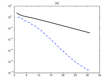
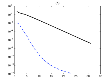
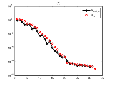
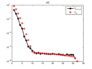
Figure 1: (a)-(b) decay rate of  $\left(\prod\nolimits_{i=1}^{m}h_{i+1,i}\right)^{1/m}$ (dash-dot line) and bound (15) (solid line), (c)-(d) decay of $h_{m+1,m}$ and $\sigma_{m}$. On the left the results for SHAW and on the right the results for WING. In each experiment $N=32$.

We need to remark that the results of Figure 1 are obtained working with the Householder implementation of the Arnoldi algorithm and hence simulating what happens in exact arithmetics.

4 The approximation of the SVD

The use of the Arnoldi algorithm as a method to approximate the marginal values of the spectrum of a matrix is widely known in literature. We may refer to [28, Chapter 6] for an exhaustive background. Using similar arguments, in this section we analyze the convergence of the singular values of the matrices $\overline{H}_{m}$ to the largest singular values of $A$. For the Lanczos bidiagonalization method [1, 26], the analysis can be done by exploiting the connection between this method and the symmetric Lanczos process (see e.g. [8]). The use of the Lanczos bidiagonalization to construct iteratively the GSVD of ($A,L$) has been studied in [17].

Let us consider the SVD factorization of $\overline{H}_{m}$, that is, $\overline{H}_{m}=U^{(m)}\Sigma^{(m)}V^{(m)T}$, $U^{(m)}\in\mathbb{R}^{\left(m+1\right)\times\left(m+1\right)}$, $V^{(m)}\in\mathbb{R}^{m\times m}$ and

$$\Sigma^{(m)}=\left(\begin{array}[]{ccc}\sigma_{1}^{(m)}&&\\ &\ddots&\\ &&\sigma_{m}^{(m)}\\ 0&\cdots&0\end{array}\right)\in\mathbb{R}^{\left(m+1\right)\times m}.$$

We can state the following results.

Proposition 6

Let $\overline{U}_{m+1}=W_{m+1}U^{(m)}\in\mathbb{R}^{N\times\left(m+1\right)}$ and $\overline{V}_{m}=W_{m}V^{(m)}\in\mathbb{R}^{N\times m}$. Then

$$\left\|A-\overline{U}_{m+1}\Sigma^{(m)}\overline{V}_{m}^{T}\right\|=\left\|A(I-W_{m}W_{m}^{T})\right\|.$$

Proof. Using (4), we have

$$A-\overline{U}_{m+1}\Sigma^{(m)}\overline{V}_{m}^{T} = A-W_{m+1}U^{(m)}\Sigma^{(m)}V^{(m)T}W_{m}^{T}$$

$$= A-W_{m+1}\overline{H}_{m}W_{m}^{T}$$

$$= A-AW_{m}W_{m}^{T}.$$

 

Observe that since $\overline{U}_{m+1}\Sigma^{(m)}=W_{m+1}\widetilde{U}^{(m)}\widetilde{\Sigma}^{(m)}$, where $\widetilde{\Sigma}^{(m)}\in\mathbb{R}^{m\times m}$ is just $\Sigma^{(m)}$ without the last row, and $\widetilde{U}^{(m)}\in\mathbb{R}^{(m+1)\times m}$ is $U^{(m)}$ without the last column, the above result states that the triplet $\left(W_{m+1}\widetilde{U}^{(m)},\widetilde{\Sigma}^{(m)},W_{m}V^{(m)}\right)$ defines an approximation of the truncated SVD of $A$, which cannot be too bad since $\left\|A(I-W_{m}W_{m}^{T})\right\|\leq\left\|A\right\|$. Moreover, it states that if the Arnoldi algorithm does not terminate before $N$ iterations, then it produces the complete SVD. The following result gives some additional information.

Proposition 7

Let $u_{k}^{(m)}\in\mathbb{R}^{m+1}$ and $v_{k}^{(m)}\in\mathbb{R}^{m}$ be respectively the right and left singular vectors relative to the singular value $\sigma_{k}^{(m)}$ of $\overline{H}_{m}$, that is, $\overline{H}_{m}v_{k}^{(m)}=\sigma_{k}^{(m)}u_{k}^{(m)}$ and $\overline{H}_{m}^{T}u_{k}^{(m)}=\sigma_{k}^{(m)}v_{k}^{(m)}$, with $1\leq k\leq m$. Then defining $\overline{u}_{k}=W_{m+1}u_{k}^{(m)}$ and $\overline{v}_{k}=W_{m}v_{k}^{(m)}$ we have that

$$A\overline{v}_{k}-\sigma_{k}^{(m)}\overline{u}_{k} = 0,$$ (23)

$$W_{m}^{T}(A^{T}\overline{u}_{k}-\sigma_{k}^{(m)}\overline{v}_{k}) = 0.$$ (24)

Proof. (23) follows directly by (4). Moreover, since

$$\overline{H}_{m}^{T}u_{k}^{(m)}-\sigma_{k}^{(m)}v_{k}^{(m)}=0,$$

using $\overline{H}_{m}^{T}=W_{m}^{T}A^{T}W_{m+1}$, and the definition of $\overline{u}_{k}$ and $\overline{v}_{k}$, we easily obtain (24).   

Remark 8

Using the square matrix $H_{m}$ to approximate the singular values of $A$, that is, computing the SVD $H_{m}=U^{(m)}\Sigma^{(m)}V^{(m)T}$, where now $U^{(m)},\Sigma^{(m)},V^{(m)}\in\mathbb{R}^{m\times m}$, if $H_{m}v_{k}^{(m)}=\sigma_{k}^{(m)}u_{k}^{(m)}$ then

$$\left\|A\overline{v}_{k}-\sigma_{k}^{(m)}\overline{u}_{k}\right\|\leq h_{m+1,m}\quad\text{with\quad}\overline{u}_{k}=W_{m}u_{k}^{(m)},\overline{v}_{k}=W_{m}v_{k}^{(m)}.$$ (25)

The above relation is very similar to the one which arises when using the eigenvalues of $H_{m}$ (the Ritz values) to approximate the eigenvalues of $A$ [28, §6.2]. Note moreover that whenever $h_{m+1,m}\approx 0$, and hence very quickly for linear ill-posed problems (see Section 3), the use of $\overline{H}_{m}$ or $H_{m}$ is almost equivalent to approximate the largest singular values of $A$.

The Galerkin condition (24) is consequence of the fact that the Arnoldi algorithm does not work with the transpose. Obviously, if $A=A^{T}$, the algorithm reduces to the symmetric Lanczos process and, under the hypothesis of Proposition 7, we easily obtain $A^{T}\overline{u}_{k}-\sigma_{k}^{(m)}\overline{v}_{k}=0$. In the general case of $A\neq A^{T}$, Proposition 7 ensures that since $\overline{v}_{k}=W_{m}v_{k}^{(m)}\in\mathcal{K}_{m}(A,b)$, by (24) the vector $\sigma_{k}^{(m)}\overline{v}_{k}$ is just the orthogonal projection of $A^{T}\overline{u}_{k}$ onto $\mathcal{K}_{m}(A,b)$, that is, $\sigma_{k}^{(m)}\overline{v}_{k}=W_{m}W_{m}^{T}A^{T}\overline{u}_{k}$, which implies

$$\left\|A^{T}\overline{u}_{k}-\sigma_{k}^{(m)}\overline{v}_{k}\right\|\leq\left\|(I-W_{m}W_{m}^{T})A^{T}W_{m}W_{m}^{T}\right\|.$$ (26)

This means that the approximation is good if $A^{T}\overline{u}_{k}$ is close to $\mathcal{K}_{m}(A,b)$. It is interesting to observe that (26) is just the ”transpose version” of (25) since

$$h_{m+1,m}=\left\|(I-W_{m}W_{m}^{T})AW_{m}W_{m}^{T}\right\|,$$

which can be easily proved using again (3) (cf. [28, Chapter 4]).

Experimentally, one observes that the Arnoldi algorithm seems to be very efficient for approximating the largest singular values for discrete ill-posed problems. In order to have a-posteriori strategy to monitor step-by-step the quality of approximation, we can state the following.

Proposition 9

Assume that the matrix $A$ has full rank. Then

$$\left\|A^{T}\overline{u}_{k}-\sigma_{k}^{(m)}\overline{v}_{k}\right\|\leq\left\|W_{m+1}^{T}AW_{m}^{\bot}\right\|,$$ (27)

where $\overline{u}_{k}$, $\overline{v}_{k}$, $\sigma_{k}^{(m)}$ are defined as in Proposition 7, and $W_{m}^{\bot}=[w_{m+1},...,w_{N}]$.

Proof. Since $\overline{v}_{k}\in\mathcal{K}_{m}(A,b)$, and $\overline{u}_{k}=W_{m+1}u_{k}^{(m)}$, by (24)

$$\left\|A^{T}\overline{u}_{k}-\sigma_{k}^{(m)}\overline{v}_{k}\right\|\leq\left\|\left(W_{m}^{\bot}\right)^{T}A^{T}W_{m+1}\right\|.$$ (28)

 

Formula (27) is rather interesting because since $h_{ij}=w_{i}^{T}Aw_{j}$ from the Arnoldi algorithm,

$$W_{m+1}^{T}AW_{m}^{\bot}=\left[\begin{array}[]{ccc}h_{1,m+1}&\cdots&h_{1,N}\\ \vdots&&\vdots\\ h_{m+1,m+1}&\cdots&h_{m+1,N}\end{array}\right].$$

Since in many cases the elements of the projected matrix $H_{m}$ tends to annihilates departing from the diagonal (this is the basic assumption of the methods based on the incomplete orthogonalization, see e.g. [29]), one may obtain useful estimates for the bound (27) working with few columns of $W_{m+1}^{T}AW_{m}^{\bot}$, that is, with few columns of $W_{m}^{\bot}$, and hence obtaining a-posteriori estimates for the quality of the SVD approximation. In order to have an experimental confirmation of this statement, in Figure 2 we show the behavior of $\left\|A-\overline{U}_{m+1}\Sigma^{(m)}\overline{V}_{m}^{T}\right\|$ and $\left\|W_{m+1}^{T}Aw_{m+1}\right\|$, for some test problems. Note that $\left\|W_{m+1}^{T}Aw_{m+1}\right\|$ comes from the bound (27) with $W_{m}^{\bot}$ replaced by $w_{m+1}.$

We remark that Proposition 5 and 9 can be used to arrest the procedure whenever the noise level $\varepsilon$ is known, since it is generally useless to continue with the SVD approximation if we find $\sigma_{k}^{(m)}<<\varepsilon$, for a certain $k$ and $m$. Indeed, in this situation the Picard condition is no longer satisfied since typically $U_{m}^{T}\approx\varepsilon$ for $m$ large enough.

For what concerns the generalized SVD of the matrix pair $(A,L)$, let $AX=US$ and $LX=VC$, where $S=diag(s_{1},...,s_{N})$ and $C=diag(c_{1},...,c_{N})$, $X\in\mathbb{R}^{N\times N}$ is nonsingular and $U,V\in\mathbb{R}^{N\times N}$ are orthogonal. Moreover let $\overline{H}_{m}X^{(m)}=U^{(m)}S^{(m)}$ and $L_{m}X^{(m)}=V^{(m)}C^{(m)}$, where $S^{(m)}=diag(s_{1}^{(m)},...,s_{m}^{(m)})$ and $C^{(m)}=diag(c_{1}^{(m)},...,c_{m}^{(m)})$, be the generalized SVD of the matrix pair $(\overline{H}_{m},L_{m})$. In this situation, for the convergence of the approximated generalized singular values and vectors, we can state the following result.

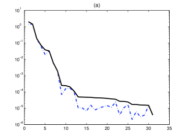
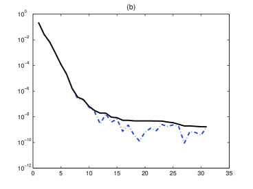
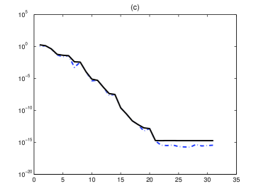
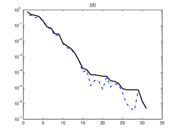
Figure 2: Decay behavior of $\left\|A-\overline{U}_{m+1}\Sigma^{(m)}\overline{V}_{m}^{T}\right\|$ (solid line) and lower bound $\left\|W_{m+1}^{T}Aw_{m+1}\right\|$ arising from Proposition 9 (dash-dot line) for BAART (a), WING (b), SHAW (c) and I_LAPLACE (d). The dimension of each problem is $N=32$.

Proposition 10

Let $u_{k}^{(m)}$, $v_{k}^{(m)}$ and $x_{k}^{(m)}$ be the $k$-th column of the matrices $U^{(m)}\in\mathbb{R}^{\left(m+1\right)\times m}$, $V^{(m)}\in\mathbb{R}^{m\times m}$ and $X^{(m)}\in\mathbb{R}^{m\times m}$ respectively. Then defining $\overline{u}_{k}=W_{m+1}u_{k}^{(m)}$, $\overline{v}_{k}=W_{m}v_{k}^{(m)}$ and $\overline{x}_{k}=W_{m}x_{k}^{(m)}$, we have

$$A\overline{x}_{k}-s_{k}^{(m)}\overline{u}_{k} = 0,$$ (29)

$$W_{m}^{T}(L\overline{x}_{k}-c_{k}^{(m)}\overline{v}_{k}) = 0.$$ (30)

Proof. Similarly to Proposition 7, (29) and (30) follows immediately from the basic relation (4).   

As before the proposition ensures that if the matrix $A$ has full rank, than the Arnoldi algorithm allows to construct the GSVD of $(A,L)$. Step by step, the quality of the approximation depends on the distance between $span\{Lw_{1},...,Lw_{m}\}$ and $\mathcal{K}_{m}(A,b)$. Similarly to (26) and (28), since $\overline{v}_{k}=W_{m}v_{k}^{(m)}\in\mathcal{K}_{m}(A,b)$, we have

$$\left\|L\overline{x}_{k}-c_{k}^{(m)}\overline{v}_{k}\right\|\leq\left\|(I-W_{m}W_{m}^{T})LW_{m}W_{m}^{T}\right\|.$$

and

$$\left\|L\overline{x}_{k}-\sigma_{k}^{(m)}\overline{v}_{k}\right\|\leq\left\|\left(W_{m}^{\bot}\right)^{T}LW_{m}\right\|.$$

In Figure 3 we show the convergence of the singular values of $\overline{H}_{m}$, and the generalized singular values of the matrix pair $\left(\overline{H}_{m},L_{m}\right)$, with

$$L=\left(\begin{array}[]{cccc}1&-1&&\\ &\ddots&\ddots&\\ &&1&-1\\ 0&\cdots&\cdots&0\end{array}\right),$$

working with the test problems SHAW and BAART. The results show that the approximations are quite accurate. It is interesting to observe that, in both cases, after 8-9 iterations the algorithm starts to generate spurious approximations. This is due to the loss of orthogonality of the Krylov vectors, since in these experiments (and in what follows) we have used the Gram-Schmidt implementation. Working with the Householder version of the algorithm the problem is fixed. Anyway in the framework of the regularization, a more accurate approximation of the smallest singular values is useless because of the error in $b$.

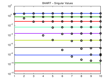
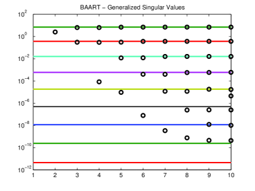
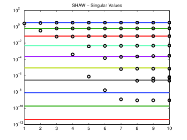
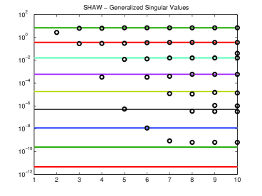
Figure 3: Plots of the singular values (circle) of the matrix $\overline{H}_{m}$ (left) and the generalized singular values of the matrix pair $(\overline{H}_{m},L_{m})$ (right) versus the iteration number k, for the problem BAART and SHAW with $N=32$. The solid lines represent the singular values of the matrix A (left) and the generalized singular values of the matrix pair $(A,L)$ (right).

5 Generalized Cross-Validation

A popular method for choosing the regularization parameter, which does non require the knowledge of the noise properties nor its norm $\left\|e\right\|$, is the Generalized Cross-Validation (GCV) [9, 32]. The major idea of the GCV is that a good choice of $\lambda$ should predict missing values, so that the model is not sensitive to the elimination of one data point. This means that the regularized solution should predict a datum fairly well, even if that datum is not used in the model. This viewpoint leads to minimization with respect to $\lambda$ of the GCV function

$$G(\lambda)=\frac{\|b-Ax_{\lambda}\|^{2}}{[\text{{trace}}(I-AA_{\lambda})]^{2}},$$

where $A_{\lambda}=(A^{T}A+\lambda^{2}L^{T}L)^{-1}A^{T}$ is the matrix that gives the regularized solutions of (2) from the normal equations

$$(A^{T}A+\lambda^{2}L^{T}L)x_{\lambda}=A^{T}b.$$

Using  the GSVD of the matrix pair $(A,L)$, with a general $\ A\in\mathbb{R}^{M\times N},L\in\mathbb{R}^{P\times N}$, let $A=USX^{-1}$ and $L=VCX^{-1}$, where $S=diag(s_{1},...,s_{P})$ and $C=diag(c_{1},...,c_{P})$, the generalized singular values $\gamma_{i}$ of $(A,L)$ are defined by the ratios

$$\gamma_{i}=\frac{s_{i}}{c_{i}},\qquad i=1,...,P.$$

Therefore, one can show that the expression of the GCV function is given by

$$G(\lambda)=\frac{\sum_{i=1}^{N}\left(\frac{\lambda^{2}}{\gamma_{i}^{2}+\lambda^{2}}u_{i}^{T}b\right)^{2}}{\left(M-(N-P)-\sum_{i=1}^{P}\frac{\gamma_{i}^{2}}{\gamma_{i}^{2}+\lambda^{2}}\right)^{2}}.$$ (31)

For the square case $M=N$, and $P\leq N$, rearranging the sum at the denominator we obtain

$$G(\lambda)=\frac{\sum_{i=1}^{N}\left(\frac{\lambda^{2}}{\gamma_{i}^{2}+\lambda^{2}}u_{i}^{T}b\right)^{2}}{\left(\sum_{i=1}^{P}\frac{\lambda^{2}}{\gamma_{i}^{2}+\lambda^{2}}\right)^{2}}.$$ (32)

The GCV criterion is then based on the choice of $\lambda$ which minimizes $G(\lambda)$. It is well known that this minimization problem is generally ill-conditioned, since the function $G(\lambda)$ is typically flat in a relatively wide region around the minimum. As a consequence, this criterion may even lead to a poor regularization [20, 22, 30].

As already said in the Introduction, for large-scale problems the GCV approach for (2) is too much expensive since it requires the SVD (GSVD). In this setting, our idea is to fully exploit the approximation properties of the Arnoldi algorithm investigated in Section 3 and 4. In particular, our aim is to define a sequence of regularization parameters $\left\{\lambda_{m}\right\}$, i.e., one for each iteration of the Arnoldi algorithm, obtained by the minimization of the following GCV function approximations

$$G_{m}(\lambda)=\frac{\left\|\overline{H}_{m}y_{m,\lambda}-\left\|b\right\|e_{1}\right\|^{2}}{\left(N-m+\sum_{i=1}^{m}\frac{\lambda^{2}}{\gamma_{i}^{(m)2}+\lambda^{2}}\right)^{2}},$$ (33)

where $y_{m,\lambda}$ solves the reduced minimization (2), and $\gamma_{i}^{(m)}$, $i=1,...,m$, are the approximations of the generalized singular values, obtained with the Arnoldi process. Note that

$$\left\|\overline{H}_{m}y_{m,\lambda}-\left\|b\right\|e_{1}\right\|^{2}=\sum_{i=1}^{m}\left(\frac{\lambda^{2}}{\gamma_{i}^{(m)2}+\lambda^{2}}u_{i}^{(m)^{T}}c\right)^{2}+\left(u_{m+1}^{(m)^{T}}c\right)^{2},$$

where $u_{i}^{(m)}$ is defined as in Proposition 10 and $c=\left\|b\right\|e_{1}$, so that the construction of $G_{m}(\lambda)$ can be obtained working in reduced dimension. The basic idea which leads to the approximation $G_{m}(\lambda)\approx G(\lambda)$, is to set equal to $0$ the generalized singular values that are not approximated by the Arnoldi algorithm, and that are expected to be close to $0$ after few iterations. This is justified by the analysis and the experiments of Section 3 and 4.

We remark that in a hybrid approach [18], one aims to regularize the projected problem

$$\min_{y\in\mathbb{R}^{m}}\left\{\left\|\overline{H}_{m}y-\left\|b\right\|e_{1}\right\|\right\}.$$ (34)

Since no geometrical information on the solution of (34) can be inherited from the solution of the original problem, the choice of $L_{m}=I_{m}$ as regularization operator is somehow forced (this is a standard strategy for hybrid methods [14, §6.7]). In this framework, if the GCV criterion is used to regularize (34), the basic difference with respect to (33) is at the denominator, where $N-m$ is replaced by $m$. We observe moreover that (33) is similar to the GCV approximation commonly used for iterative methods, in which the denominator is simply $N-m$ [14, §7.4].

In the following, the algorithm that has been used for the tests of the next sections.

AT - GCV Algorithm

given $A\in{\mathbb{R}}^{N\times N},\;b\in{\mathbb{R}}^{N}$, $\delta$
while $\big{|}\left\|r_{m}\right\|-\left\|r_{m-1}\right\|\big{|}/\left\|r_{m}\right\|\geq\delta$
	update $\overline{H}_{m}$ and $L_{m}$ from (5) and (9)
	compute GSVD($\overline{H}_{m},L_{m}$)
	compute $\lambda_{m}=\arg\min_{\lambda}G_{m}(\lambda$)
	solve $\min_{y_{m}\in\mathbb{R}^{m}}\left\|\left(\begin{array}[]{c}\overline{H}_{m}\\ \lambda_{m}L_{m}\end{array}\right)y_{m}-\left(\begin{array}[]{c}\left\|b\right\|e_{1}\\ 0\end{array}\right)\right\|^{2}$
	compute the corresponding residual $r_{m}$
end
compute $x_{m}=W_{m}y_{m}$

The stopping rule used in the algorithm is just based on the residual. As an alternative, one may even employ the strategy adopted in [4], based on the observation of the GCV approximations.

6 Numerical results

In order to test the performance of the proposed method, we consider again some classical test problems taken from the Regularization Tools [15]. In particular in Figures 4-5, we consider the problems BAART, SHAW, FOXGOOD, I_LAPLACE, with right-hand side affected by 0.1% or 1% Gaussian noise. The regularization operator is always the discretized first derivative, augmented with a zero row at the bottom to make it square (cf. (9)). For each experiment we show: (a) the approximation of $G(\lambda)$ obtained with the functions $G_{m}(\lambda)$ for some values of $m$, with a graphical comparison of the local minima; (b) the approximate solution; (c) the relative residual and error history; (d) the sequence of selected parameters $\left\{\lambda_{m}\right\}$, with respect to the one obtained with the minimization of $G(\lambda)$ (denoted by $\lambda_{A}$ in the pictures) and the optimal one ($\lambda_{opt}$) obtained by the minimization of the distance between the regularized and the true solution [25]

$$\min_{\lambda}\left\|x_{reg}-x_{true}\right\|^{2}\equiv\min_{\lambda}f(\lambda),$$

where

$$f(\lambda)=\left\{\sum_{i=1}^{p}\left(\frac{\lambda^{2}}{(\gamma_{i}^{2}+\lambda^{2})}\frac{u_{i}^{T}b}{\sigma_{i}}x_{i}-\sum_{i=p+1}^{N}(u_{i}^{T}b)x_{i}\right)-\sum_{i=1}^{N}\frac{u_{i}^{T}b}{\sigma_{i}}v_{i}\right\}^{2}.$$

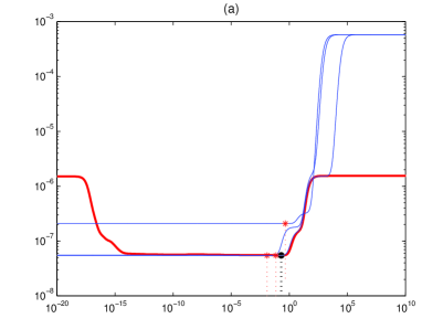
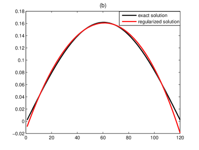
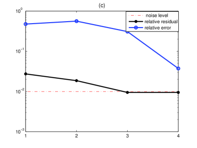
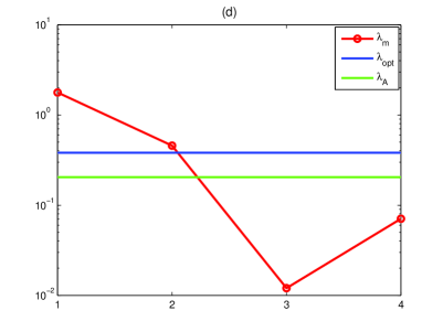
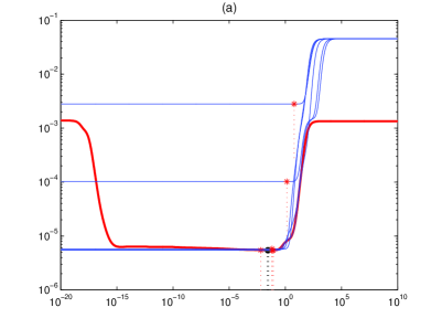
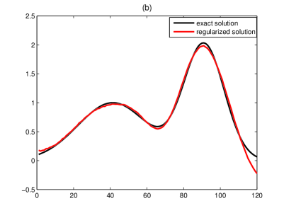
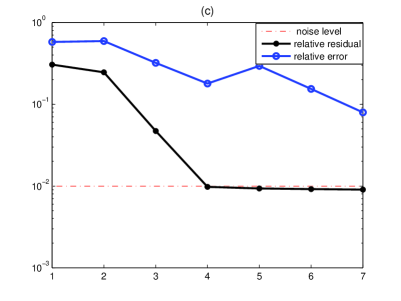
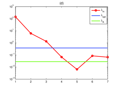
Figure 4: Results for BAART (top) and SHAW (bottom). The dimension of each problem is $N=120$. Noise level $\varepsilon=10^{-2}.$

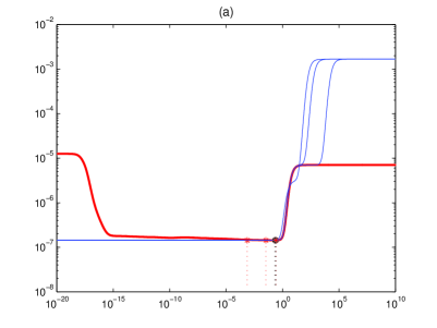
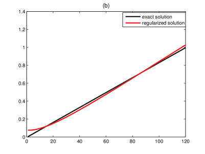
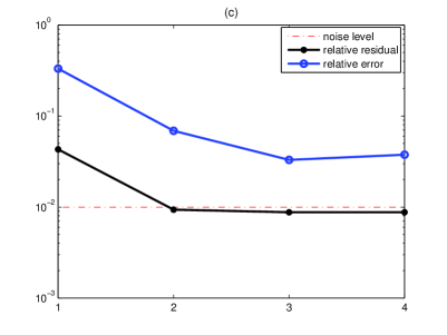
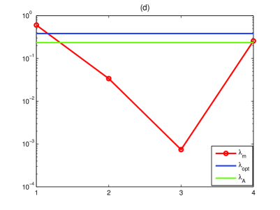
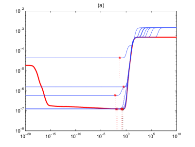
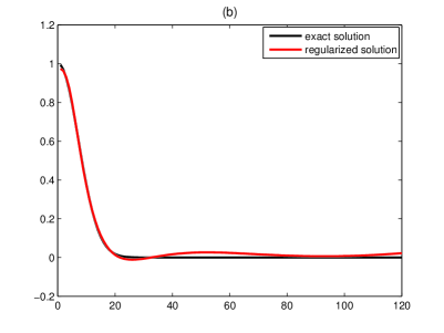
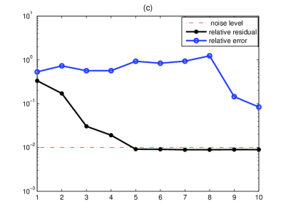
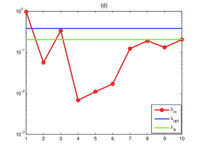
Figure 5: Results for FOXGOOD (top) and I_LAPLACE (bottom). The dimension of each problem is $N=120$. Noise level $\varepsilon=10^{-3}.$

7 An example of image restoration

We conclude with an illustration of the performance of the GCV-Arnoldi approach on a 2D image deblurring problem which consist in recovering the original $n\times n$ image from a blurred and noisy observed image.

Let $X$  be a $n\times n$ two dimensional image. The vector $\overline{x}$ of dimension $N=n^{2}$ obtained by stacking the columns of the image $X$ represents a blur-free and noise-free image. We generate an associated blurred and noise-free image $\overline{b}$ by multiplying $\overline{x}$ by a block Toeplitz matrix $A\in\mathbb{R}^{N\times N}$ with Toeplitz blocks, implemented in the function blur.m from the Regularization Tools [15]. This Matlab function has two parameters, band and sigma; the former specifies the half-bandwidth of the Toeplitz blocks and the latter the variance of the Gaussian point spread function. The blur and noise contaminated image $b\in\mathbb{R}^{N}$ is obtained by adding a noise-vector $e\in\mathbb{R}^{N}$, so that $b=A\overline{x}+e$. We assume the blurring operator $A$ and the corrupted image $b$ to be available while no information is given on the error $e$, we would like to determine a restoration which accurately approximates the blur-free and noise-free image $\overline{x}$.

We consider the restoration of a corrupted version of the $256\times 256$ test image mri.png. Contamination is by 1% white Gaussian noise and space-invariant Gaussian blur. The latter is generated as described above with blur parameters band=7, sigma=2, so that the condition number of $A$ is around $10^{13}$. Figure 6 displays the performance of the AT-GCV. On the left the blur-free and noise-free image, on the middle the corrupted image, on the right the restored image. From top to bottom the image in original size and two different zooms. The regularization operator is defined as (cf. [7])

$$L=I_{n}\otimes L_{1}+L_{1}\otimes I_{n}\in\mathbb{R}^{N\times N},$$

where $L_{1}\in\mathbb{R}^{n\times n}$ is the discretized first derivative with a zero row at the bottom (cf. also [17, §5]).

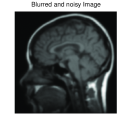
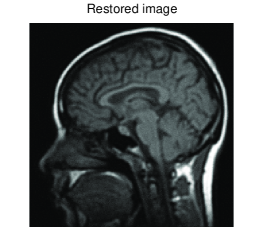
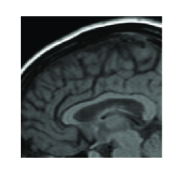
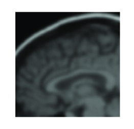
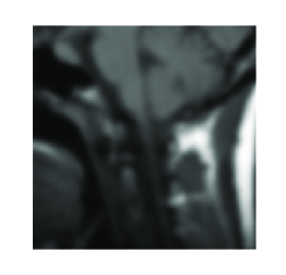
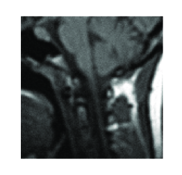
Figure 6: Restoration of mri.png image. Original image, blurred and noisy image with noise level $\varepsilon=10^{-2}$ and blur parameters band=7, sigma=2, restored image. From top to bottom original size and two zoom.

The experiment has been carried out using Matlab 7.10 on a single processor computer (Intel Core i7). The result has been obtained in 5 iterations of the Arnoldi algorithm, in around $0.5$ seconds. Many other experiments on image restoration have shown similar performances.

8 Conclusion

The fast convergence of the Arnoldi algorithm when applied to compact operators makes the AT method particularly attractive for the regularization of discrete ill-posed problems. The projected problems rapidly inherit the basic features of the original one, allowing a substantial computational advantage with respect to other approaches.

In this paper, in absence of information on the noise which affects the right-hand side of the system, we have employed the GCV criterion. Contrary to the hybrid techniques, the sequence of regularization parameters $\left\{\lambda_{m}\right\}_{m\geq 1}$ is defined in order to regularize the original problem instead of the projected one, leading to GCV approximations which are similar to the ones used for pure iterative methods ([14, §7.4]). Notwithstanding the intrinsic difficulties concerning the GCV criterion, the arising algorithm has shown to be quite robust. Of course there are cases in which the method fails, but the numerical experiments presented are rather representative of what happens in general.

References

- [1] A. Bjorck, A bidiagonalization algorithm for solving large and sparse ill-posed systems of linear equations, BIT 28, 659–670 (1988).
- [2] F. Bauer, M. Lukas, Comparing parameter choice methods for regularization of ill-posed problems, Math. Comput. Simulation 81(9), 1795–1841 (2011).
- [3] D. Calvetti, S. Morigi, L. Reichel, F.Sgallari, Tikhonov regularization and the L-curve for large discrete ill-posed problems, J. Comput. Appl. Math. 123, 423–446 (2000) .
- [4] J.Chung, J.G. Nagy, D.P. O’Leary, A weighted-GCV method for Lanczos-hybrid regularization, Electron. Trans. Numer. Anal. 28, 149–167 (2007/08).
- [5] M. Donatelli, A. Neuman, and L. Reichel, Square regularization matrices for large linear discrete ill-posed problems, Numer. Linear Algebra Appl. 19, 896–913 (2012).
- [6] J. N. Franklin, Minimum Principles for Ill-Posed Problems, SIAM Journal on Math. Anal. 9(4), 638–650 (1978).
- [7] S. Gazzola, P. Novati, Automatic parameter setting for Arnoldi-Tikhonov methods. Submitted 2012.
- [8] G.H. Golub, F. T. Luk, M. L. Overton, A Block Lánczos Method for Computing the Singular Values of Corresponding Singular Vectors of a Matrix, ACM Trans. Math. Software, 7(2), 149–169 (1981).
- [9] G.H. Golub, M. Heath, G. Wahba, Generalized cross-validation as a method for choosing a good ridge parameter, Technometrics 21(2), 215–223 (1979).
- [10] U. Hämarik, R. Palm, T. Raus, A family of rules for parameter choice in Tikhonov regularization of ill-posed problems with inexact noise level, J. Comput. Appl. Math. 236(8), 2146–2157 (2012).
- [11] M. Hanke, On Lanczos based methods for the regularization of discrete ill-posed problems, BIT 41, 1008–1018 (2001).
- [12] P.C. Hansen, The discrete Picard condition for discrete ill-posed problems, BIT 30, 658–672 (1990).
- [13] M. Hanke, P.C. Hansen, Regularization methods for large-scale problems, Surv. Math. Ind. 3, 253–315 (1993).
- [14] P.C. Hansen, Rank-Deficient and Discrete Ill-Posed Problems: Numerical Aspects of Linear Inversion. SIAM, Philadelphia (1998).
- [15] P.C. Hansen, Regularization Tools Version 4.0 for Matlab 7.3, Numer. Algorithms 46, 189–194 (2007).
- [16] B. Hofmann, Regularization for Applied Inverse and Ill-Posed Problems. Teubner, Stuttgart, Germany (1986).
- [17] M.E. Kilmer, P.C. Hansen, M.I. Español, A projection-based approach to general-form Tikhonov regularization, SIAM J. Sci. Comput. 29(1), 315–330 (2007).
- [18] M.E. Kilmer, D.P. O’Leary, Choosing regularization parameters in iterative methods for ill-posed problems, SIAM J. Matrix Anal. Appl. 22, 1204–1221 (2001).
- [19] S. Kindermann, Convergence analysis of minimization-based noise levelfree parameter choice rules for linear ill-posed problems, Electron. Trans. Numer. Anal. 38, 233–257 (2011).
- [20] R. Kohn, C.F. Ansley, D. Tharm, The performance of cross-validation and maximum likelihood estimators of spline smoothing parameters, J. Am. Stat. Assoc. 86 , 1042–1050 (1991).
- [21] B. Lewis, L. Reichel, Arnoldi-Tikhonov regularization methods, J. Comput. Appl. Math. 226, 92–102 (2009).
- [22] M.A. Lukas, Robust generalized cross-validation for choosing the regularization parameter, Inverse Probl. 22, 1883–1902 (2006).
- [23] I, Moret. A note on the superlinear convergence of GMRES, SIAM J. Numer. Anal. 34(2), 513–516 (1997).
- [24] O. Nevanlinna, Convergence of Iterations for Linear Equations. Birkhäuser, Basel (1993).
- [25] D.P. O’Leary, Near-optimal parameters for Tikhonov and other regularization methods, SIAM J. Sci. Comput. 23(4), 1161–1171 (2011).
- [26] D.P. O’Leary, J.A. Simmons, A bidiagonalization-regularization procedure for large-scale discretizations of ill-posed problems, SIAM J. Sci. Statist. Comput. 2, 474–489 (1981).
- [27] L. Reichel, G. Rodriguez, Old and new parameter choice rules for discrete ill-posed problems, Numer. Algorithms, 2012. DOI: 10.1007/s11075-012-9612-8. Available online.
- [28] Y. Saad, Numerical methods for large eigenvalue problems. Algorithms and Architectures for Advanced Scientific Computing. Manchester University Press, Manchester, Halsted Press, New York (1992).
- [29] Y. Saad, K. Wu, DQGMRES: a direct quasi-minimal residual algorithm based on incomplete orthogonalization, Numer. Linear Algebra Appl. 3, 329–343 (1996).
- [30] A.M. Thompson, J.W. Kay, D.M. Titterington, A cautionary note about crossvalidatory choice, J. Stat. Comput. Simul. 33, 199–216 (1989).
- [31] L. N. Trefethen, D. Bau, Numerical Linear Algebra. SIAM, Philadelphia (1997).
- [32] G. Wahba, A comparison of GCV and GML for choosing the smoothing parameter in the generalized spline smoothing problem, Ann. Stat. 13, 1378–1402 (1985).