Branched Spherical CR structures on the complement of the figure eight knot.

Abstract.

We obtain a branched spherical CR structure on the complement of the figure eight knot whose holonomy representation was given in [4]. There are essentially two boundary unipotent representations from the complement of the figure eight knot into $\mathbf{PU}(2,1)$, we call them $\rho_{1}$ and $\rho_{2}$. We make explicit some fundamental differences between these two representations. For instance, seeing the figure eight knot complement as a surface bundle over the circle, the behaviour of of the fundamental group of the fiber under the representation is a key difference between $\rho_{1}$ and $\rho_{2}$.

1. Introduction

The three dimensional sphere contained in $\mathbb{C}^{2}$ inherits a Cauchy-Riemann structure as the boundary of the complex two-ball. Three dimensional manifolds locally modeled on the sphere then are called spherical CR manifolds and have been studied since Cartan ([2]). Spherical CR structures appear naturally as quotients of an open subset of the three dimensional sphere by a subgroup of the CR automorphism group (denoted $\mathbf{PU}(2,1)$) (see [7, 6] and [11] for a recent introduction).

The irreducible representations of the fundamental group of the complement of the figure eight knot into $\mathbf{PU}(2,1)$ with unipotent boundary holonomy were obtained in [4]. To obtain such representations, one imposes the existence of a developing map obtained from the 0-skeleton of an ideal triangulation. Solution of a system of algebraic equations gives rise to a set of representations of $\Gamma=\pi_{1}(M)$, the fundamental group of the complement of the figure eight knot with parabolic peripheral group.

Up to pre-composition with automorphisms of $\Gamma$ there exists 2 irreducible representations into $\mathbf{PU}(2,1)$ with unipotent boundary holonomy (see [3]). Following [4] we call them $\rho_{1}$ and $\rho_{2}$. In [4] we showed that $\rho_{1}$ could be obtained from a branched spherical CR structure on the knot complement. Moreover, this representation is not the holonomy of a complete structure as the limit set is the full sphere $S^{3}$.

In this paper we analyze $\rho_{2}$ and show that it is also obtained as the holonomy of a branched structure in Theorem 12 in section 6. The proof consists of extending the developing map obtained from the 0-skeleton to a developing map defined on simplices. A complete (non-branched) spherical CR structure on the complement of the figure eight knot was obtained in [3]. Although the complete structure with unipotent boundary holonomy is unique (see [3]), it is not clear to us how to describe all branched structures. The motivation to study branched CR structures is the hope that they would be easier to associate to a manifold once a representation is given. As we have a general method to construct representations of the fundamental group into $\mathbf{PU}(2,1)$ we would like an efficient method to obtain spherical CR structures with holonomy the given representation. Constructing branched structures might be a step in this process. Remark that a complete structure in the Whitehead link complement is described in [11] and, more recently, a whole family in [9].

Another motivation for this paper is to stress a major difference between the two representations $\rho_{1}$ and $\rho_{2}$. Recall that the fundamental group of the figure eight knot complement contains a surface group (a punctured torus group) as a normal subgroup corresponding to the fundamental group of the fiber of the fibration of the complement over a circle. In fact the kernel of the first representation is contained in the surface group (and is not finitely generated) but the kernel of the second one is not. This, in turn, implies that the image of the surface group is of infinite index in the image of $\rho_{1}$ but of finite index in the image of $\rho_{2}$. Both images of the representations are contained in arithmetic lattices as infinite index subgroups. It turns out that the limit set of the image of $\rho_{1}$ is the full $S^{3}$ but the image of $\rho_{2}$ has a proper limit set (see [3]). These properties are given in sections 4.1 and 4.2. They might be general properties of representations of 3-manifold groups into $\mathbf{PU}(2,1)$.

We thank M. Deraux, A. Guilloux, A. Reid, P. Will and M. Wolff for fruitful discussions.

2. Complex hyperbolic space and its boundary.

In this section, we introduce some basic materials about complex hyperbolic geometry. We refer Goldman’s book [6] for details.

2.1. Complex hyperbolic space and its isometry group.

Let $\mathbb{C}^{2,1}$ be the three dimensional complex vector space equipped with the Hermitian form

$$\langle Z,W\rangle=Z_{1}\overline{W}_{3}+Z_{2}\overline{W}_{2}+Z_{3}\overline{W}_{1}.$$

One has three subspaces:

$$V_{+}=\{Z\in\mathbb{C}^{2,1}:\langle Z,Z\rangle>0\},$$

$$V_{0}=\{Z\in\mathbb{C}^{2,1}-\{0\}:\langle Z,Z\rangle=0\},$$

$$V_{-}=\{Z\in\mathbb{C}^{2,1}:\langle Z,Z\rangle<0\}.$$

Let $P:\mathbb{C}^{2,1}-\{0\}\rightarrow\mathbb{C}P^{2}$ be the canonical projection onto complex projection space. Then complex hyperbolic 2-space is defined as $\mathbf{H}^{2}_{\mathbb{C}}=P(V_{-})$ equipped with the Bergman metric. The boundary of complex hyperbolic space is defined as $\partial\mathbf{H}^{2}_{\mathbb{C}}=P(V_{0})$.

Let $\mathbf{U}(2,1)$ be the linear matrix group preserving the Hermitian form $\langle.,.\rangle$. The holomorphic isometry group $\mathbf{PU}(2,1)$ of $\mathbf{H}^{2}_{\mathbb{C}}$ is the projection of the unitary group $\mathbf{U}(2,1)$. The isometry group of $\mathbf{H}^{2}_{\mathbb{C}}$ is

$$\widehat{\mathbf{PU}(2,1)}=\langle\mathbf{PU}(2,1),Z\mapsto\overline{Z}\rangle,$$

where $Z\mapsto\overline{Z}$ is the complex conjugation.

The elements of $\mathbf{PU}(2,1)$ can be classified into three kinds of classes. Any element $g\in\mathbf{PU}(2,1)$ is called loxodromic if $g$ fixes exactly two points in $\partial\mathbf{H}^{2}$; $g$ is called parabolic if it fixes exactly one point in $\partial\mathbf{H}^{2}$; otherwise, $g$ is called elliptic.

2.2. Lattices.

Let ${\mathcal{O}}_{d}$ be the ring of integers in the imaginary quadratic number field ${\mathbb{Q}}(i\sqrt{d})$ where $d$ is a positive square-free integer. If $d\equiv 1,2$ (mod 4) then ${\mathcal{O}}_{d}=\mathbb{Z}[i\sqrt{d}]$ and if $d\equiv 3$ (mod 4) then ${\mathcal{O}}_{d}=\mathbb{Z}[\frac{1+i\sqrt{d}}{2}]$. The subgroup of ${\mathbf{PU}(2,1)}$ with entries in ${\mathcal{O}}_{d}$ is called the Picard modular group for ${\mathcal{O}}_{d}$ and is written ${\mathbf{PU}}(2,1;{\mathcal{O}}_{d})$. They are arithmetic lattices first considered by Picard.

2.3. Heisenberg group and $\mathbb{C}-$circles

The Heisenberg group $\mathfrak{N}$ is defined as the set $\mathbb{C}\times\mathbb{R}$ with group law

$$(z,t)\cdot(z^{\prime},t^{\prime})=(z+z^{\prime},t+t^{\prime}+2\rm{Im}(z\overline{z}^{\prime})).$$

The boundary of complex hyperbolic space $\partial\mathbf{H}^{2}_{\mathbb{C}}$ can be identified with the one point compactification $\overline{\mathfrak{N}}$ of $\mathfrak{N}$.

A point $p=(z,t)\in\mathfrak{N}$ and the point at infinity are lifted to the following points in $\mathbb{C}^{2,1}$:

$$\hat{p}=\left[\begin{array}[]{c}(-|z|^{2}+it)/2\\ z\\ 1\end{array}\right]\quad\rm{and}\quad\hat{\infty}=\left[\begin{array}[]{c}1\\ 0\\ 0\end{array}\right].$$

There are two kinds of totally geodesic submanifolds of real dimension 2 in $\mathbf{H}^{2}_{\mathbb{C}}$: complex geodesics and totally real totally geodesic planes. Their boundaries in $\partial\mathbf{H}^{2}_{\mathbb{C}}$ are called $\mathbb{C}-$circles and $\mathbb{R}-$circles. Complex geodesics can be parametrized by their polar vectors, that is, points in $P(\mathbb{C}^{2,1})$ which are projections of vectors orthogonal to the lifted complex geodesic.

Proposition 2.1.

In the Heisenberg model, $\mathbb{C}-$circles are either vertical lines or ellipses, whose projection on the z-plane are circles.

For a given pair of distinct points in $\partial\mathbf{H}^{2}_{\mathbb{C}}$, there is a unique $\mathbb{C}-$circle passing through them. Finite $\mathbb{C}-$circles are determined by a centre and a radius. For example, the finite $\mathbb{C}-$circle with centre $(z_{0},t_{0})$ and radius $R>0$ has polar vector

$$\left[\begin{array}[]{c}(R^{2}-|z_{0}|^{2}+it_{0})/2\\ z_{0}\\ 1\\ \end{array}\right]$$

and in which any point $(z,t)$ satisfies the equations

$$\left\{\begin{array}[]{ll}|z-z_{0}|=R\\ t=t_{0}+2\rm{Im}(\overline{z}z_{0})\end{array}\right.$$

2.4. CR structures

CR structures appear naturally as boundaries of complex manifolds. The local geometry of these structures was studied by E. Cartan [2] who defined, in dimension three, a curvature analogous to curvatures of a Riemannian structure. When that curvature is zero, Cartan called them spherical CR structures and developed their basic properties. A much later study by Burns and Shnider [1] contains the modern setting for these structures.

Definition 2.1.

A spherical CR-structure on a 3-manifold is a geometric structure modeled on the homogeneous space $S^{3}$ with the above ${\mathbf{PU}(2,1)}$ action.

Definition 2.2.

We say a spherical CR-structure on a 3-manifold is complete if it is equivalent to a quotient of the domain of regularity in $S^{3}$ by a discrete subgroup of ${\mathbf{PU}(2,1)}$.

Here, equivalence between CR structures is defined, as usual, by diffeomorphisms preserving the structure. The diffeomorphism group of a manifold therefore acts trivially on its CR structures. Observe that taking the complex conjugate of local charts of a CR structure (maps of open sets into $S^{3}$) gives another CR structure which might not be equivalent to the original one. A weaker definition of spherical CR structures as geometric structures modeled on the full isometry group $\widehat{{\mathbf{PU}(2,1)}}$ with its action on $S^{3}$ is sometimes preferable. Indeed, in that case, complex conjugation of local charts will induce an equivalent spherical CR structure.

A CR structure, in particular, has an orientation which is compatible with the orientation induced by its contact structure. Observe that even $\widehat{{\mathbf{PU}(2,1)}}$ preserves orientation so a spherical CR structure in the weaker sense is also oriented. Both orientations of $S^{3}$ are obtained via equivalent CR structures because there exists an orientation reversing diffeomorphism of $S^{3}$. More generally, manifolds which have orientation reversing maps either have equivalent CR structures opposite orientations or none. On the other hand, It is not clear if a manifold having a CR structure will have another one giving its opposite orientation.

As all geometric structures, a spherical structure on a manifold $M$ induces a developing map defined on its universal cover $\tilde{M}$

$$d:\tilde{M}\rightarrow S^{3}$$

and a holonomy representation

$$\rho:\pi_{1}(M)\rightarrow{\mathbf{PU}(2,1)}.$$

Observe again that pre-composition with a diffeomorphism will induce an equivalent structure with a holonomy representation which is obtained from the old one by pre-composition with an automorphism of the fundamental group. Also observe that the holonomy representation is not discrete in general and the developping map might be surjective.

2.5. Branched structures

Given a representation is not clear that it is defined as the holonomy representation of a spherical CR structure. In that sense it is useful to introduce a weaker definition of branched structure in the hope that representations might be understood in a geometric way.

A branched spherical CR structure is a CR structure except along some curves where the structure is locally modeled on the $t$-axis inside $\mathbb{R}^{3}=\{\ (z,t)\ |\ z\in\mathbb{C},t\in\mathbb{R}\ \}$ together with the ramified map into the Heisenberg group given by

$$(z,t)\rightarrow(z^{n},t),$$

where $n$ is the branching order. The CR structure around the curve is given by the pullback of the CR structure around the Heisenberg $t$-axis.

3. The figure eight knot.

We use the same notations as that in the paper [4] and recall briefly the three irreducible representations obtained there.

The figure eight knot complement $M$ has a fundamental group $\Gamma=\pi_{1}(M)$ which can be presented as

$$\Gamma=\langle\ g_{1},g_{3}\ |\ [g_{3},g_{1}^{-1}]g_{3}=g_{1}[g_{3},g_{1}^{-1}]\ \rangle.$$

It is useful to introduce another generator

$$g_{2}=[g_{3},g_{1}^{-1}],$$

that is

$$g_{1}=g_{2}g_{3}g_{2}^{-1}.$$

The figure eight knot complement is fibered over the circle with fiber a punctured torus. The fibration is encoded in the following sequence.

$$1\rightarrow F_{2}\rightarrow\Gamma\rightarrow\mathbb{Z}\rightarrow 0$$

Here, $F_{2}$ is the free group of rank 2 with generators

$$F_{2}=\langle\ a=g_{2},b=[g_{2},g_{3}^{-1}]\ \rangle.$$

We can then present

$$\Gamma=\langle\ a,b,t\ |\ tat^{-1}=aba,tbt^{-1}=ab\ \rangle.$$

where $t=g_{3}$ is seen to act as a pseudo-Anosov element of the mapping class group of $F_{2}$.

We consider in this paper the following representations into $\mathbf{SU}(2,1)$ obtained in [4]:

1. $$\rho_{1}(g_{1})=\begin{pmatrix}1&1&-\frac{1}{2}-\frac{\sqrt{3}}{2}i\\ 0&1&-1\\ 0&0&1\\ \end{pmatrix},\ \ \rho_{1}(g_{3})=\begin{pmatrix}1&0&0\\ 1&1&0\\ -\frac{1}{2}-\frac{\sqrt{3}}{2}i&-1&1\\ \end{pmatrix}.$$

2. $$\rho_{2}(g_{1})=\begin{pmatrix}1&1&-\frac{1}{2}-\frac{\sqrt{7}}{2}i\\ 0&1&-1\\ 0&0&1\\ \end{pmatrix},\ \ \rho_{2}(g_{3})=\begin{pmatrix}1&0&0\\ -1&1&0\\ -\frac{1}{2}+\frac{\sqrt{7}}{2}i&1&1\\ \end{pmatrix}.$$

3. $$\rho_{3}(g_{1})=\begin{pmatrix}1&1&-1/2\\ 0&1&-1\\ 0&0&1\\ \end{pmatrix},\ \ \rho_{3}(g_{3})=\begin{pmatrix}1&0&0\\ \frac{5}{4}-\frac{\sqrt{7}}{4}i&1&0\\ -1&-\frac{5}{4}-\frac{\sqrt{7}}{4}i&1\\ \end{pmatrix}.$$

The representation $\rho_{3}$ is obtained by pre-composition of $\rho_{2}$ with the automorphisms of the fundamental group associated to a reversing orientation diffeomorphism. So we will concentrate in the first two representations during the rest of this paper.

4. Representations

As every complement of a tame knot, the complement of the figure eight knot has fundamental group $\Gamma$ fitting in the exact sequence

$$1\rightarrow[\Gamma,\Gamma]\rightarrow\Gamma\rightarrow\mathbb{Z}\rightarrow 0.$$

In the case of the complement of the figure eight knot we have

$$1\rightarrow F_{2}\rightarrow\Gamma\rightarrow\mathbb{Z}\rightarrow 0$$

where $F_{2}$ is the free group of rank two. We will be interested in the general case when

$$1\rightarrow F\rightarrow\Gamma\rightarrow\mathbb{Z}\rightarrow 0$$

is an exact sequence. Suppose

$$\rho:\Gamma\rightarrow G$$

is a representation with $K=Ker(\rho)$.

Lemma 1.

The following diagram is commutative:

$$\begin{CD}111\\ @V{}V{}V@V{}V{}V@ VVV\\ 1@>{}>{}>K\cap F@>{}>{}>K@>{p}>{}>p(K)@>{}>{}>0\\ @V{}V{}V@V{}V{}V@ VVV\\ 1@>{}>{}>F@>{}>{}>\Gamma @>{p}>{}>\mathbb{Z}@>{}>{}>0\\ @V{\rho}V{}V@V{\rho}V{}V@ V\bar{\rho}VV\\ 1@>{}>{}>\rho(F)@>{}>{}>\rho(\Gamma)@>{\bar{p}}>{}>\rho(\Gamma)/\rho(F)@>{}>{}>0\\ @V{}V{}V@V{}V{}V@ VVV\\ 111\end{CD}$$

Where $\bar{p}$ is the quotient map and $\bar{\rho}$ is defined so that the diagram be commutative.

Proof.  The only verification we have to make is that $Ker(\bar{\rho})$ is the image of $p(K)$. Suppose $x=p(ft^{n})\in Ker(\bar{\rho})$ with $t\in p^{-1}(1)$, $n\in\mathbb{Z}$ and $f\in F$ satisfying

$$\bar{p}\rho(ft^{n})=Id.$$

Then $\rho(ft^{n})=\rho(f^{\prime})$ with $f^{\prime}\in F$. Therefore ${f^{\prime}}^{-1}ft^{n}\in K$ and then $x=p(ft^{n})=p({f^{\prime}}^{-1}ft^{n})\in p(K)$.      

We conclude that the inclusion $\rho(F)\subset\rho(\Gamma)$ is of finite index if and only if $K$ contains an element $ft^{n}$,$n\neq 0$, where $f\in F$ and $p(t)=1$. The index is precisely the least absolute value of an integer satisfying the condition.

Corollary 2.

$\rho(F)\lhd\rho(\Gamma)$ is of infinite index if and only if $K\subset F$.

4.1.

The representation $\rho_{1}$.

We consider the first representation. Let $\omega_{3}=-\frac{1}{2}+i\frac{\sqrt{3}}{2}$. The ring of integers of the field $Q(i\sqrt{3})$ is ${\mathcal{O}}_{3}=\mathbb{Z}[\omega_{3}]$. The representation is discrete, since the generators $G_{1},G_{2},G_{3}$ are contained in the arithmetic lattice $P_{3}=PU(2,1;{\mathcal{O}}_{3})$.

We use the presentation of $P_{3}$ obtained in [5]:

$$P_{3}=\langle P,Q,I\ |\ I^{2}=(QP^{-1})^{6}=PQ^{-1}IQP^{-1}I=P^{3}Q^{-2}=(IP)^{3}\ \rangle.$$

Recall from [4] that $\rho_{1}(\Gamma)$ is generated by

$$G_{1}=[P,Q]\ ,$$

$$G_{2}=[I,[Q,P]]\ ,$$

$$G_{3}=A[P,Q]A^{-1}\ ,$$

with $A=P^{-2}IP^{2}$.

A usefull tool in the following computations is the normalizer $N=N(\rho_{1}(\Gamma))\subset P_{3}$, the least normal subgroup of $P_{3}$ containing $\rho_{1}(\Gamma)$.

Lemma 3 ([4]).

$P_{3}/N$ is isomorphic to $\mathbb{Z}/6\mathbb{Z}$.

Computing that $P_{3}/[P_{3},P_{3}]$ is of order 6 and observing that $[P_{3},P_{3}]\subset N$ we remark that $N=[P_{3},P_{3}]$. By computing the quotient of $P_{3}$ by the normalizer of $\langle G_{1},I,[Q,P^{-1}]\rangle$ we obtain the following

Lemma 4 ([4]).

$N=\langle G_{1},I,[Q,P^{-1}]\rangle.$

Lemma 5.

$P_{3}/[N,N]$ is isomorphic to the euclidean triangle group of type $(2,3,6)$.

Proof.  Using the presentation of $P_{3}$ and the lemma above we obtain for the presentation of the quotient

$$P_{3}/[N,N]=\langle P,Q\ |\ (QP^{-1})^{6}=P^{3}=Q^{2}\ \rangle.$$

     

Lemma 6.

$N/[N,N]$ is isomorphic to $\mathbb{Z}\oplus\mathbb{Z}$.

Proof.  From the isomorphism theorem

$$N/[N,N]=\frac{P_{3}/[N,N]}{P_{3}/N}$$

and the two previous lemmas we obtain the result.      

We have (cf. [4])

$$[\rho_{1}(\Gamma),\rho_{1}(\Gamma)]\lhd\rho_{1}(\Gamma)\lhd\langle G_{1},I\rangle\lhd N\lhd PU(2,1;{\mathcal{O}}_{3})$$

with the last inclusion of order 6 and the inclusion $\rho_{1}(\Gamma)\lhd\langle G_{1},I\rangle$ of index at most two.

Observe now that the inclusion $\langle G_{1},I\rangle\lhd N$ has abelian quotient and therefore $[N,N]\subset\langle G_{1},I\rangle$ so we obtain

$$[\rho_{1}(\Gamma),\rho_{1}(\Gamma)]\subset[N,N]\lhd\langle G_{1},I\rangle\lhd N\lhd PU(2,1;{\mathcal{O}}_{3})$$

The following Proposition was obtained after discussions with A. Reid. The proof given here is a simplification of his argument which involved a gap computation ([10]).

Proposition 4.1.

The inclusions

$$[\rho_{1}(\Gamma),\rho_{1}(\Gamma)]\lhd\rho_{1}(\Gamma)\subset PU(2,1;{\mathcal{O}}_{3})$$

are of infinite index.

Proof.  Observe first that $[\rho_{1}(\Gamma),\rho_{1}(\Gamma)]\lhd\langle G_{1},I\rangle$ and $[N,N]\lhd\langle G_{1},I\rangle$ are two normal inclusions and therefore

$$\langle G_{1},I\rangle/[N,N]\rightarrow\langle G_{1},I\rangle/[\rho_{1}(\Gamma),\rho_{1}(\Gamma)]$$

is a monomorphism. On the other hand, the quotient $\langle G_{1},I\rangle/[\rho_{1}(\Gamma),\rho_{1}(\Gamma)]$ is finite or contains $\mathbb{Z}$ as a subgroup of index at most two.

Suppose now that $\rho_{1}(\Gamma)\subset PU(2,1;\mathbb{Z}[\omega])$ is of finite index. Then $\langle G_{1},I\rangle\lhd N$ should be of finite index and therefore, as $N/[N,N]=\mathbb{Z}\oplus\mathbb{Z}$, $\langle G_{1},I\rangle/[N,N]=\mathbb{Z}\oplus\mathbb{Z}$. This contradicts the monomorphism above.

Suppose next that $[\rho_{1}(\Gamma),\rho_{1}(\Gamma)]\lhd\rho_{1}(\Gamma)$ is of finite index. Then the inclusion $[\rho_{1}(\Gamma),\rho_{1}(\Gamma)]\lhd\langle G_{1},I\rangle$ would be of finite index. This, in turn, implies that $[N,N]\lhd\langle G_{1},I\rangle$ is of finite index. Now this contradicts the monomorphism

$$N/[N,N]\rightarrow N/\langle G_{1},I\rangle$$

as $N/\langle G_{1},I\rangle$ is abelian of rank at most one.      

From Lemma 1 and Proposition 4.1 we obtain the following

Corollary 7.

$$Ker(\rho_{1})\lhd[\Gamma,\Gamma].$$

We conclude with the following property of the kernel:

Proposition 4.2.

$Ker(\rho_{1})$ is not of finite type.

Proof.  Observe that $Ker(\rho_{1})$ is clearly preserved under the pseudo-anosov element of the mapping class group denoted by $t$. The result then follows from Lemme 6.2.5 in [8].      

4.2.

The representation $\rho_{2}$.

The second representation (see the subsection 6.5.1 in [4]) is given by $\Gamma_{2}=\rho_{2}(\pi_{1}(M))$, with $\Gamma_{2}=\langle\rho_{2}(g_{1}),\rho_{2}(g_{2}),\rho_{2}(g_{3})\rangle$, where

$$G_{1}:=\rho_{2}(g_{1})=\left(\begin{array}[]{ccc}1&1&-\frac{1}{2}-i\frac{\sqrt{7}}{2}\\ 0&1&-1\\ 0&0&1\\ \end{array}\right)$$

$$G_{2}:=\rho_{2}(g_{2})=\left(\begin{array}[]{ccc}2&\frac{3}{2}-i\frac{\sqrt{7}}{2}&-1\\ -\frac{3}{2}-i\frac{\sqrt{7}}{2}&-1&0\\ -1&0&0\\ \end{array}\right)$$

$$G_{3}:=\rho_{2}(g_{3})=\left(\begin{array}[]{ccc}1&0&0\\ -1&1&0\\ -\frac{1}{2}+i\frac{\sqrt{7}}{2}&1&1\\ \end{array}\right).$$

Moreover, $G_{2}=[G_{3},G_{1}^{-1}]$ is a regular elliptic element of order four, and $G_{1},G_{3}$ are pure parabolic elements.

Remark 4.1.

We can also see that the element $G_{3}G_{1}^{-1}$ is loxodromic. The fixed points of $G_{1},G_{3}$ are respectively $p_{1}=\infty$ and $p_{2}=(0,0)$.

Let $\omega_{7}=\frac{1}{2}+i\frac{\sqrt{7}}{2}$. The ring of integers of the field $Q(i\sqrt{7})$ is ${\mathcal{O}}_{7}=\mathbb{Z}[\omega_{7}]$. We observe then that the representation is discrete, since the generators $G_{1},G_{2},G_{3}$ are contained in the arithmetic lattice $PU(2,1;{\mathcal{O}}_{7})$.

Theorem 8 (see Proposition 3.3 and Theorem 4.4 in [12]).

The group $PU(2,1;{\mathcal{O}}_{7})$ is generated by the elements

$$I=\left(\begin{array}[]{ccc}0&0&1\\ 0&-1&0\\ 1&0&0\\ \end{array}\right),R_{1}=\left(\begin{array}[]{ccc}1&0&0\\ 0&-1&0\\ 0&0&1\\ \end{array}\right),R_{2}=\left(\begin{array}[]{ccc}1&1&-\bar{\omega_{7}}\\ 0&-1&1\\ 0&0&1\\ \end{array}\right),$$

$$R_{3}=\left(\begin{array}[]{ccc}1&\bar{\omega_{7}}&-1\\ 0&-1&\omega_{7}\\ 0&0&1\\ \end{array}\right),T=\left(\begin{array}[]{ccc}1&0&i\sqrt{7}\\ 0&1&0\\ 0&0&1\\ \end{array}\right).$$

Moreover, the stabilizer subgroup of infinity has the presentation

$$\langle R_{1},R_{2},R_{3},T|R_{1}^{2}=R_{3}^{2}=[T,R_{1}]=[T,R_{3}]=TR_{2}^{-2}=(R_{1}R_{3}R_{2})^{2}=Id\rangle.$$

We may express the generators of $\rho_{2}(\Gamma)$ in terms of the generators of $PU(2,1;{\mathcal{O}}_{7})$:

Proposition 4.3.

$$G_{1}=R_{1}R_{2}T^{-1}=R_{1}R_{2}^{-1},$$

$$-G_{2}=R_{2}R_{1}R_{3}I,$$

$$G_{3}=IR_{2}IR_{1}=IR_{2}R_{1}I=IG_{1}^{-1}I.$$

We also observe that

$$\rho_{2}(\Gamma)=\langle G_{1},G_{2},G_{3}\rangle=\langle G_{1},G_{3}\rangle\lhd\langle G_{1},I\rangle$$

where $\langle G_{1},G_{3}\rangle\lhd\langle G_{1},I\rangle$ is a subgroup of index at most two since $G_{3}=IG_{1}^{-1}I$.

We also have

Lemma 9.

$$\langle G_{1},I,T\rangle\lhd\langle G_{1},I,T,R_{1}\rangle=PU(2,1;{\mathcal{O}}_{7})$$

Proof.  $\langle G_{1},I,T\rangle\lhd\langle G_{1},I,T,R_{1}\rangle$ is a normal subgroup since $R_{1}G_{1}R_{1}=T^{-1}G_{1}^{-1}$, $R_{1}IR_{1}=I$ and $R_{1}TR_{1}=T$. The normal inclusion is of index at most two.      

The inclusion

$$\langle G_{1},I\rangle\subset\langle G_{1},I,T\rangle$$

can be neither normal nor finite if one proves that the limit set is not $S^{3}$.

A simple computation shows that

Lemma 10.

$$\rho_{2}(t^{3})=[\rho_{2}(a^{-1}),\rho_{2}(b^{-1})]$$

From the lemma above and Lemma 2 we obtain

Corollary 11.

$$[\rho_{2}(\Gamma),\rho_{2}(\Gamma)]\lhd\rho_{2}(\Gamma)$$

is of index at most three.

5. Tetrahedra

5.1. Edges

Given two points $p_{1}$ and $p_{2}$ in $S^{3}$, there exists a unique $\mathbb{C}$-circle between them. As the boundary of a complex disc has a positive orientation, the $\mathbb{C}$-circle inherits that orientation and defines therefore two distinct arcs $[p_{1},p_{2}]$ and $[p_{2},p_{1}]$ (see Figure 1).

// // size(4cm,0); //defaultpen(1); // usepackage(”amssymb”); //import geometry; // On d finit un r el et trois points. real h=5; pair O=(0,0),A=(-h,0),B=(h,0); // On trace le demi-cercle de diam tre [AB] // en tournant dans le sens direct de B vers A. draw(arc(O,B,A),blue,MidArrow(5bp));draw(arc(O,A,B),red,MidArrow(5bp)); // Et on ajoute les points. dot(”$p_{1}$”,A,SW); dot(”$p_{2}$”,B,SE);

draw(Label(”$[p_{2},p_{1}]$”,Relative(1/3),align=NE),arc(O,B,A)); draw(Label(”$[p_{1},p_{2}]$”,Relative(1/3),align=SW),arc(O,A,B));

Figure 1. A $\mathbb{C}$-circle between two points in $S^{3}$ is oriented and defines two oriented segments.

The complex disc is contained in complex hyperbolic space and does not intersect $S^{3}$ except in the boundary. If one wants to obtain a disc in $S^{3}$ whose boundary is a $\mathbb{C}$-circle, a usefull construction is obtained by using a family of $\mathbb{C}$-circles which foliates the disc. It could have a singularity at one point in the interior or at the boundary. Remark though that this construction is not canonical.

5.2. Triangles

Given three points $p_{1},p_{2},p_{3}\in S^{3}$ we might construct six different triangles (1-skeletons) corresponding to an orientation choice of the edges between the points. Observe that if the three points are contained in the same $\mathbb{C}$-circle some edges contain two vertices. If we suppose, on the other hand, that the three points are not in the same $\mathbb{C}$-circle (we refer to it as a generic configuration) then the three edges (any choice) intersect only at the vertices.

In order to obtain a surface whose boundary is the triangle we might fix one point $p\in S^{3}$ and consider the segments (of $\mathbb{C}$-circles) joining that point and the edges as in a barycentric construction. If the orientation of the edges permits, one can degenerate this construction making $p$ approach one of the vertices (it is clear that this is not possible only if the edges define an orientation of the triangle). There are choices to be made in that construction and each choice corresponds to a different triangle.

It is easier to analyse first the case where the triangle is degenerate: If the vertices are generic the triangle defined above is embedded. In the case of an oriented triangle, we could add first an edge complement of one of the edges (making a full $\mathbb{C}$-circle) and then consider a degenerate triangle with that edge union a disc whose boundary is the full $\mathbb{C}$-circle now foliated by $\mathbb{C}$-circles with singular point one of the vertices.

It is not clear from the definition that the surface defined is embedded. Each case needs a verification.

// // size(3cm,0); //defaultpen(1); // usepackage(”amssymb”); //import geometry; real h=5; path e2=(-h,0)..(-h,-5)..(0,-2*h); path e1=(0,-2*h)..(h,-5)..(h,0); draw(e2,blue,MidArrow(5bp));draw(e1,blue,MidArrow(5bp));

// On d finit un r el et quatre points. pair O=(0,0),A=(-h,0),B=(h,0),D=(0,-2*h); // On trace le demi-cercle de diam tre [AB] // en tournant dans le sens direct de B vers A. draw(arc(O,B,A),blue,MidArrow(5bp));draw(arc(O,A,B),red,MidArrow(5bp));

// Et on ajoute les points. dot(”$p_{1}$”,A,SW); dot(”$p_{2}$”,B,SE); dot(”$p_{3}$”,D,SW); //draw(Label(”$[p_{2},p_{1}]$”,Relative(1/3),align=NE),arc(O,B,A)); //draw(Label(”$[p_{1},p_{2}]$”,Relative(1/3),align=SW),arc(O,A,B));

Figure 2. Triangles. We show four possible edges given a configuration of three points.

// // size(3cm,0); //defaultpen(1); // usepackage(”amssymb”); //import geometry; real h=5; path e2=(-h,0)..(-h,-5)..(0,-2*h); path e1=(0,-2*h)..(h,-5)..(h,0); draw(e1,blue,MidArrow(5bp));draw(e2,blue,MidArrow(5bp));

// On d finit un r el et quatre points. pair O=(0,0),A=(-h,0),B=(h,0),D=(0,-2*h); // On trace le demi-cercle de diam tre [AB] // en tournant dans le sens direct de B vers A. //draw(arc(O,B,A),blue,MidArrow(5bp)); draw(arc(O,A,B),blue,MidArrow(5bp));

// Et on ajoute les points. dot(”$p_{1}$”,A,SW); dot(”$p_{2}$”,B,SE); dot(”$p_{3}$”,D,SW);

// Le 2-squelete pair u1=(-2,-h-.5); pair u2=(-3.5,-h-1);

path uu=A..u1..point(e1,1); path uu2=A..u2..point(e1,.3); draw(uu,MidArrow(5bp));draw(uu2,MidArrow(5bp));

Figure 3. Triangles. A 2-skeleton foliated by arcs in $\mathbb{C}$-circles.

// // size(3cm,0); //defaultpen(1); // usepackage(”amssymb”); //import geometry; real h=5; path e2=(-h,0)..(-h,-5)..(0,-2*h); path e1=(0,-2*h)..(h,-5)..(h,0); draw(e2,blue,MidArrow(5bp));draw(e1,blue,MidArrow(5bp));

// On d finit un r el et quatre points. pair O=(0,0),A=(-h,0),B=(h,0),D=(0,-2*h); // On trace le demi-cercle de diam tre [AB] // en tournant dans le sens direct de B vers A. draw(arc(O,B,A),blue,MidArrow(5bp));draw(arc(O,A,B),MidArrow(5bp));

// Et on ajoute les points. dot(”$p_{1}$”,A,SW); dot(”$p_{2}$”,B,SE); dot(”$p_{3}$”,D,SW);

// Le 2-squelete pair u1=(-2,-h-.5); pair u2=(-3.5,-h-1);

path uu=A..u1..point(e1,1); path uu2=A..u2..point(e1,.3); draw(uu,MidArrow(5bp));draw(uu2,MidArrow(5bp));

draw(circle((-h+2*h/3,0),2*h/3),Arrow(5bp));draw(circle((-h+h/2,0),h/2),Arrow(4bp));draw(circle((-h+h/3,0),h/3),Arrow(3bp));

Figure 4. Triangles. A 2-skeleton foliated by arcs in $\mathbb{C}$-circles. The case where the degenerate barycentric construction does not apply.

5.3. CR Tetrahedra

Once faces whose border are triangles are defined one can define a 3-simplex based on a configuration of four points by choosing faces to each of the four configurations of three points. The problem is that the choices have to be compatible and faces, otherwise well defined, could intersect between one another.

We will make arguments using sometimes flat discs adjoined to edges keeping in mind that we could, in fact, by a slight deformation deal with 3-simplices.

Definition 5.1.

A tetrahedron is called a generalized tetrahedron if it has a disc adjoined to an edge. That is is a simplex union a disc whose intersection with the simplex is an edge contained in the boundary of the disc.

We could deform then these faces thickening the disc to obtain a topological 3-simplex. Faces of tetrahedra are not canonical and we will make use of this flexibility.

6. Branched CR structures associated to representations.

The representations in [4] are obtained by imposing that the 0-skeleton of an ideal triangulation defines a developing map. The triangulation of the figure eight knot complement is shown in Figure 5. The 0-skeleton can be realized as points in $S^{3}$ and using the side pairing maps we can define a developing map on the 0-skeleton of the universal covering.

In order to obtain a spherical CR structure we have to define the 1-skeleton, the 2-skeleton, then obtain 3-simplices and show that the developing map defined on the 0-skeleton extends to the 3-simplices.

Once we obtain two 3-simplices in $S^{3}$ which have well defined side pairings we might have some branching along the edges of the simplices. In fact we will prove that around one of the edges the simplices are put together as in Figure 7 but along the other edge we show that the 6 tetrahedra turn around the edge three times.

// // size(10cm); defaultpen(1); usepackage(”amssymb”); import geometry;

// point o = (8,0); point oo = (24,0); pair ph = (10,0); pair pv = (5,8);

// draw(o – o+pv,Arrow(5bp,position=.4), Arrow(5bp,position=.5)); draw(o+pv – o+ph, Arrow(5bp,position=.6)); draw(o+ph-pv– o, Arrow(5bp,position=.6)); draw(o+ph-pv– o+ph, Arrow(5bp,position=.6)); draw(o+ ph/2+(0,.2)–o+pv, Arrow(5bp,position=.4), Arrow(5bp,position=.5)); draw(o+ph-pv – o+ph/2+ (0,-.2)); draw(o – o+ph,Arrow(5bp,position=.3), Arrow(5bp,position=.4) );

label(”$3$”, o, 1*W);

label(”$4$”, o+ph, .6*E);

label(”$1$”, o+pv, 1*N); label(”$2$”, o+ph -pv, 1*S);

// draw( oo+pv – oo,Arrow(5bp,position=.6)); draw( oo+pv – oo+ph,Arrow(5bp,position=.6)); draw( oo+ph-pv – oo,Arrow(5bp,position=.6)); draw(oo+ ph/2+(0,.2)–oo +pv,Arrow(5bp,position=.4), Arrow(5bp,position=.5)); draw(oo+ph-pv – oo+ ph/2-(0,.2)); draw(oo+ph-pv – oo+ ph,Arrow(5bp,position=.5),Arrow(5bp,position=.6)); draw(oo – oo+ph,Arrow(5bp,position=.3), Arrow(5bp,position=.4));

label(” $3$”, oo, 1*W);

label(” $4$”, oo+ph, .6*E);

label(” $1$”, oo+pv, 1*N);

label(”$2$”, oo+ph -pv, 1*S);

Figure 5. The figure eight represented by two tetrahedra with face pairings defined by the set of arrows.

// // size(8cm); defaultpen(1); usepackage(”amssymb”); import geometry;

// point o = (8,0); pair ph = (10,0); pair pv = (5,8);

pair pq3 = (3,1); //

// draw(o – o+pv,Arrow(5bp,position=.4), Arrow(5bp,position=.5)); draw(o+pv – o+ph, Arrow(5bp,position=.6)); draw(o+ph-pv– o, Arrow(5bp,position=.6)); draw(o+ph-pv– o+ph, Arrow(5bp,position=.6)); draw(o+ ph/2+(0,.2)–o+pv, Arrow(5bp,position=.4), Arrow(5bp,position=.5)); draw(o+ph-pv – o+ph/2+ (0,-.2)); draw(o – o+ph,Arrow(5bp,position=.3), Arrow(5bp,position=.4) );

// draw(o+pv – o+ph+pq3, Arrow(5bp,position=.6)); draw(o+ph-pv– o+ph+pq3,Arrow(4bp,position=.4), Arrow(4bp,position=.5)); draw(o+ph– o+ph+pq3,Arrow(3bp,position=.3), Arrow(3bp,position=.4));

// //label(”$q_{1}$”, o, 1*W);

//label(”$q_{2}$”, o+ph, 2*dir(145)); label(”$q_{3}$”, o+ph+pq3, .6*E);

//label(”$p_{1}$”, o+pv, 1*N);

//label(”$p_{2}$”, o+ph -pv, 1*S);

Figure 6. A schematic view of the two tetrahedra glued along one face.

// // size(8cm); defaultpen(1); usepackage(”amssymb”); import geometry;

// point o = (8,0); pair ph = (10,0); pair pv = (5,8);

pair pq3 = (3,1); //pair q4 = (-3,1); //pair q5 = (-10,0); //pair q6= (-3,-1); //

// draw(o – o+pv,Arrow(5bp,position=.4), Arrow(5bp,position=.5)); draw(o+pv – o+ph, Arrow(5bp,position=.6)); draw(o+ph-pv– o, Arrow(5bp,position=.6)); draw(o+ph-pv– o+ph, Arrow(5bp,position=.6)); draw(o+ ph/2+(0,.2)–o+pv, Arrow(5bp,position=.4), Arrow(5bp,position=.5)); draw(o+ph-pv – o+ph/2+ (0,-.2)); draw(o – o+ph,Arrow(5bp,position=.3), Arrow(5bp,position=.4) );

// draw(o+pv – o+ph+pq3); draw(o+ph-pv– o+ph+pq3); draw(o+ph– o+ph+pq3);

// draw(o+ph+pq3– o+ph+pq3 +q4,linewidth(.5bp)); draw(o+ph+pq3+q4– o+ph+pq3 +q4+q5,linewidth(.5bp)); draw(o+ph+pq3+q4 +q5– o+ph+pq3 +q4+q5+q6,linewidth(.5bp)); draw(o+ph+pq3+q4 +q5+q6– o);

draw(o+pv – o+ph+pq3 +q4,linewidth(.5bp)); draw(o+pv – o+ph+pq3 +q4+q5,linewidth(.2bp)); draw(o+pv – o+ph+pq3 +q4+q5+q6,linewidth(.2bp));

draw(o+ph-pv – o+ph+pq3 +q4,linewidth(.2bp)); draw(o+ph-pv – o+ph+pq3 +q4+q5,linewidth(.2bp)); draw(o+ph-pv – o+ph+pq3 +q4+q5+q6,linewidth(.2bp));

// //label(”$q_{1}$”, o, .7*dir(115));

//label(”$q_{2}$”, o+ph, 2*dir(145)); label(”$q_{3}$”, o+ph+pq3, .6*E); label(”$q_{4}$”, o+ph+pq3 +q4, .6*dir(45)); label(”$q_{5}$”, o+ph+pq3+q4+q5, .6*NW); label(”$q_{6}$”, o+ph+pq3+q4+q5+q6, .6*W);

//label(”$p_{1}$”, o+pv, 1*N);

//label(”$p_{2}$”, o+ph -pv, 1*S);

Figure 7. A schematic view of the six tetrahedra glued around the edge $[p_{1},p_{2}]$.

6.1. The representation $\rho_{2}$

In this section, we consider the second representation. Our main theorem is

Theorem 12.

The representation $\rho_{2}$ is discrete and is the holonomy of a branched spherical CR structure on the complement of the figure eight knot.

The discreteness of the representation follows from the observation that $\rho_{2}(\Gamma)$ is contained in a lattice. To prove the existence of a spherical CR structure on the complement of the figure eight knot, it suffices to construct two tetrahedra in the Heseinberg space with side pairings which allow the definition of a developing map.

The rest of this section is will be devoted to the construction of the two tetrahedra in the Heseinberg space and to verify the conditions so that the developing map be well defined. The difficulty of this construction is that we don’t have a canonical way to define the 2-skeleton. The definitions of the faces are made so that they satisfy the necessary intersection properties.

We use half of a $\mathbb{C}$-circle to construct the segment between two given points. For a given pair points in the Heisenberg space $p$ and $q$, we use the $[p,q]$ to denote the segment connecting the two points with the direction from $p$ to $q$.

6.2. The 0-skeleton and the side parings.

The tetrahedra are $T_{1}:=[p_{1},p_{2},q_{1},q_{2}]$ and $T_{2}:=[p_{1},p_{2},q_{2},q_{3}]$, where

$$p_{1}=\infty,p_{2}=(0,0),q_{1}=(1,\sqrt{7}),$$

$$q_{2}=(\frac{5}{4}+i\frac{\sqrt{7}}{4},0),q_{3}=(\frac{1}{4}+i\frac{\sqrt{7}}{4},-\frac{\sqrt{7}}{2}).$$

The side paring transformations are

$$g_{1}:(q_{2},q_{1},p_{1})\rightarrow(q_{3},p_{2},p_{1})$$

$$g_{2}:(p_{2},q_{1},q_{2})\rightarrow(p_{1},q_{2},q_{3})$$

$$g_{3}:(q_{1},p_{2},p_{1})\rightarrow(q_{2},p_{2},q_{3})$$

There are 6 tetrahedra around the edge $[p_{2},p_{1}]$ (see Figure 7) and $[p_{2},q_{2}]$ respectively. They are obtained by translating $T_{1}$ and $T_{2}$. They are:

$$T_{1},T_{2},G_{1}(T_{1}),G_{1}G_{3}^{-1}(T_{2}),G_{1}G_{3}^{-1}G_{2}(T_{1}),G_{1}G_{3}^{-1}G_{2}G_{1}^{-1}(T_{2}),$$

and respectively

$$T_{1},T_{2},G_{3}(T_{1}),G_{3}G^{-1}_{2}(T_{2}),G_{3}G^{-1}_{2}(T_{1}),G_{3}G^{-1}_{2}G^{-1}_{1}(T_{2}).$$

Following the side parings, it is easy to see the following:

1. $G_{1}(q_{2},q_{1},p_{1})=(q_{3},p_{2},p_{1})$.

2. $G_{1}G_{3}^{-1}(q_{2},p_{2},q_{3})=(p_{2},q_{4},p_{1})$ with

   $$q_{4}=G_{1}(p_{2})=(-1,-\sqrt{7}).$$

3. $G_{1}G_{3}^{-1}G_{2}(p_{2},q_{1},q_{2})=(q_{5},p_{2},p_{1})$ with

   $$q_{5}=G_{1}G_{3}^{-1}(p_{1})=\left(\frac{-5}{4}+i\frac{\sqrt{7}}{4},0\right).$$

4. $G_{1}G_{3}^{-1}G_{2}G_{1}^{-1}(q_{3},p_{2},p_{1})=(p_{1},p_{2},q_{6})$ with

   $$q_{6}=G_{1}G_{3}^{-1}G_{2}(p_{1})=\left(-\frac{1}{4}+i\frac{\sqrt{7}}{4},\frac{\sqrt{7}}{2}\right)$$

   and $G_{1}G_{3}^{-1}G_{2}G_{1}^{-1}(q_{2})=q_{1}$.

5. Since $G_{1}G_{3}^{-1}G_{2}G_{1}^{-1}G_{3}(q_{1},p_{2},p_{1})=(q_{1},p_{2},p_{1})$, $G_{1}G_{3}^{-1}G_{2}G_{1}^{-1}G_{3}=Id$.

And,

1. $G_{3}(p_{2},q_{1},q_{2})=(p_{2},q_{2},p_{3})$ with

   $$p_{3}=G_{3}(q_{2})=\left(\frac{23}{32}+i\frac{5\sqrt{7}}{32},-\frac{\sqrt{7}}{16}\right).$$

2. $G_{3}G^{-1}_{2}(p_{1},p_{2},q_{2})=(p_{2},p_{4},q_{2})$ with

   $$p_{4}=G_{3}G^{-1}_{2}(p_{2})=\left(\frac{5}{8}+i\frac{\sqrt{7}}{8},0\right).$$

3. $G_{3}G^{-1}_{2}(p_{1},q_{1},q_{2})=(p_{2},p_{5},q_{2})$ with

   $$p_{5}=G_{3}G^{-1}_{2}(q_{1})=\left(\frac{3}{4}+i\frac{\sqrt{7}}{4},0\right).$$

4. $G_{3}G^{-1}_{2}G^{-1}_{1}(p_{1},q_{2},q_{3})=(p_{2},q_{1},q_{2}).$

5. Since $G_{3}G^{-1}_{2}G^{-1}_{1}G_{2}(p_{2},q_{1},q_{2})=(p_{2},q_{1},q_{2})$, $G_{3}G^{-1}_{2}G^{-1}_{1}G_{2}=Id$.

6.3. The 1-skeleton:

In fact, considering the orientations of the edges, there are four possibilities for the choice of the one skeleton. Here, we consider one choice given in Figure 8. Precisely, $[p_{2},p_{1}]=(0,t)$ with $t\leq 0$ and

$$[p_{2},q_{2}]=\left(\frac{5+i\sqrt{7}}{8}+\frac{\sqrt{2}}{2}e^{i\theta},\frac{1}{8}\left(\sqrt{14}\cos(\theta)-5\sqrt{2}\sin(\theta)\right)\right),$$

where $\theta\in\left[\arccos\left(\frac{5\sqrt{2}}{8}\right),2\pi-\arccos\left(-\frac{5\sqrt{2}}{8}\right)\right]$. The other edges are determined from these two by applying the side-pairings.

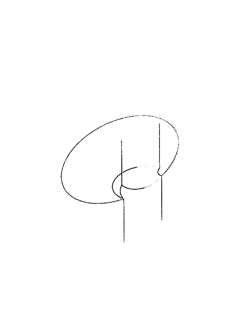
(a) The space view

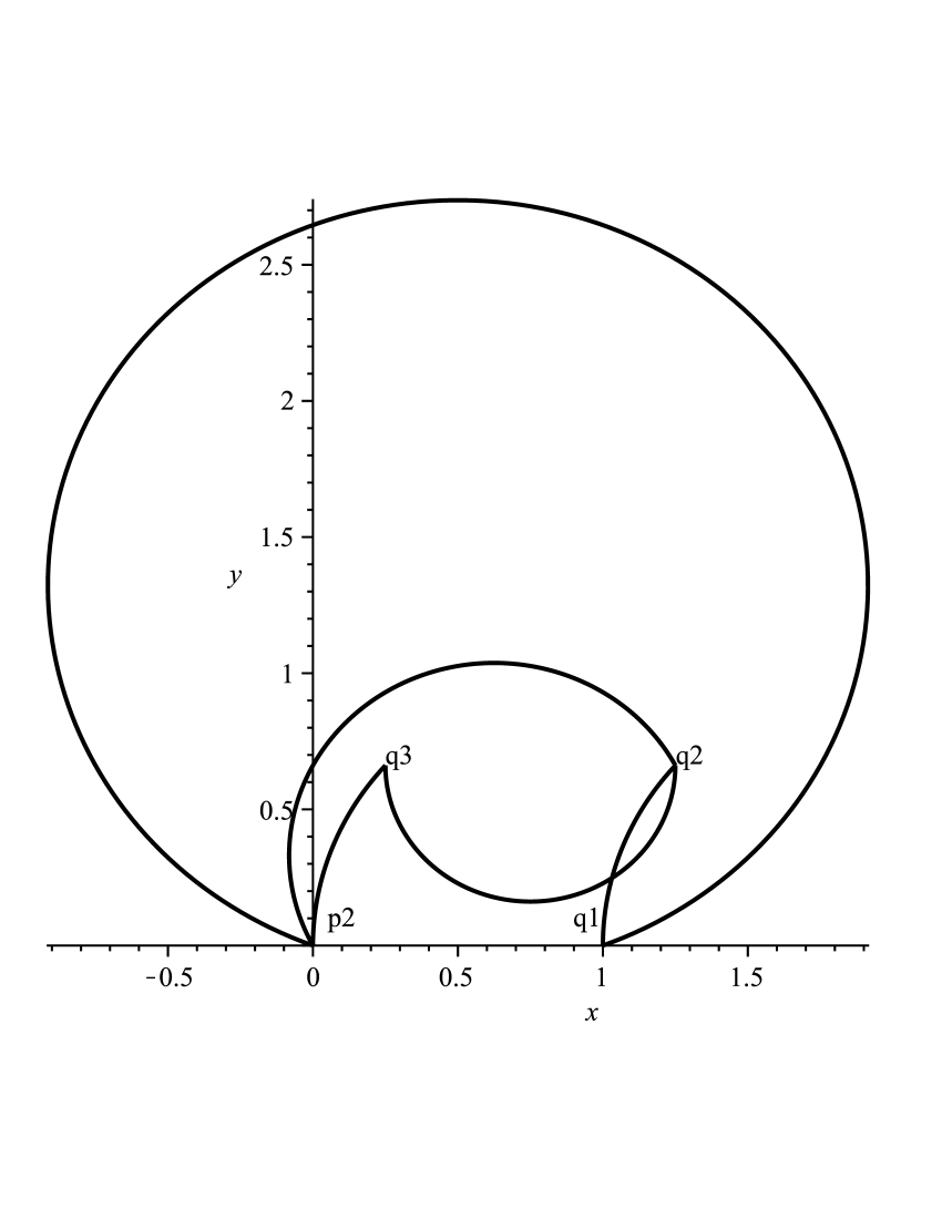
(b) The projected view

Figure 8. The one skeleton of the tetrahedra

6.4. The 2-skeleton

In this subsection, we give the details of the construction of the faces of the two tetrahedra.

6.4.1. Faces of $T_{1}$:

// // size(10cm); //defaultpen(1); usepackage(”amssymb”); import geometry;

// point o = (8,0); point oo = (24,0); pair ph = (10,0); pair pv = (5,8); point c= (13,3); point cc= (29,3);

// draw(o – o+pv, Arrow(5bp,position=.5)); draw(o+pv – o+ph, Arrow(5bp,position=.6),Arrow(5bp,position=.5)); draw(o – o+ph,Arrow(5bp,position=.5) ); dot(”$v_{1}$”,c,S);

path v1=c..o+pv; path v2=c..o+ph; path v3=o..c; draw(v1,MidArrow(3bp));draw(v2,MidArrow(3bp));draw(v3,MidArrow(3bp));

//path uu2=A..u2..point(e1,.3); //draw(uu,MidArrow(3bp)); //draw(uu2,MidArrow(3bp));

// label(”$p_{2}$”, o, 1*W); label(”$q_{2}$”, o+ph, .6*E); label(”$q_{1}$”, o+pv, 1*N);

// draw(oo– oo+pv,Arrow(5bp,position=.5),Arrow(5bp,position=.6)); draw( oo+ph–oo+pv,Arrow(5bp,position=.5),Arrow(5bp,position=.6)); draw(oo – oo+ph,Arrow(5bp,position=.5)); dot(”$v_{3}$”,cc,SW);

path hor=oo – oo+ph; dot(”$v_{2}$”,point(hor,.5),S); path hor=oo – oo+ph; //path u1=cc..u2..point(e1,.3); path u1=cc..oo+pv; path u2=cc..oo+ph; path u3=point(hor,.5)..cc; draw(u1,MidArrow(3bp));draw(u2,MidArrow(3bp));draw(u3,MidArrow(3bp));

// label(” $p_{2}$”, oo, 1*W); label(” $q_{1}$”, oo+ph, .6*E); label(” $p_{1}$”, oo+pv, 1*N);

Figure 9. A schematic view of faces $F(p_{2},q_{1},q_{2})$ (left) and $F(p_{1},p_{2},q_{1})$ (right).

// // size(4cm,0); //defaultpen(1); // usepackage(”amssymb”); //import geometry; real h=5;

path e2=(-h,0)..(-h,-5)..(0,-2*h); path e1=(0,-2*h)..(h,-5)..(h,0); path ie1=(h,0)..(h,-5)..(0,-2*h);//

draw(e2,MidArrow(5bp)); draw(ie1,Arrow(Relative(.7),size=1.7mm),Arrow(Relative(.6),size=1.7mm));

// On d finit un r el et quatre points. pair O=(0,0),A=(-h,0),B=(h,0),D=(0,-2*h); // On trace le demi-cercle de diam tre [AB] // en tournant dans le sens direct de B vers A.

draw(arc(O,B,A),MidArrow(5bp),Arrow(Relative(.6),size=1.8mm)); draw(arc(O,A,B),MidArrow(3bp));

// Et on ajoute les points. dot(”$p_{1}$”,A,SW); dot(”$q_{1}$”,B,SE); dot(”$q_{2}$”,D,SW);

// Le 2-squelete pair u1=(-2,-h-.5); pair u2=(-3.5,-h-1);

path uu=A..u1..point(e1,1); path uu2=A..u2..point(e1,.3); draw(uu,MidArrow(3bp)); draw(uu2,MidArrow(3bp));

draw(circle((-h+2*h/3,0),2*h/3),Arrow(3bp)); draw(circle((-h+h/2,0),h/2),Arrow(3bp)); draw(circle((-h+h/3,0),h/3),Arrow(3bp));

Figure 10. A schematic view of the face $F(p_{1},q_{1},q_{2})$.

// // size(4cm,0); //defaultpen(1); // usepackage(”amssymb”); //import geometry; real h=5;

path e2=(-h,0)..(-h,-5)..(0,-2*h); path e1=(0,-2*h)..(h,-5)..(h,0);

draw(e2,MidArrow(5bp)); draw(e1,MidArrow(5bp));

// On d finit un r el et quatre points. pair O=(0,0),A=(-h,0),B=(h,0),D=(0,-2*h); // On trace le demi-cercle de diam tre [AB] // en tournant dans le sens direct de B vers A.

draw(arc(O,B,A),MidArrow(5bp),Arrow(Relative(.6),size=1.8mm)); draw(arc(O,A,B),MidArrow(3bp));

// Et on ajoute les points. dot(”$p_{1}$”,A,SW); dot(”$p_{2}$”,B,SE); dot(”$q_{2}$”,D,SW);

// Le 2-squelete pair u1=(-2,-h-.5); pair u2=(-3.5,-h-1);

path uu=A..u1..point(e1,1); path uu2=A..u2..point(e1,.3); draw(uu,MidArrow(3bp)); draw(uu2,MidArrow(3bp));

draw(circle((-h+2*h/3,0),2*h/3),Arrow(3bp)); draw(circle((-h+h/2,0),h/2),Arrow(3bp)); draw(circle((-h+h/3,0),h/3),Arrow(3bp));

Figure 11. A schematic view of the face $F(p_{1},p_{2},q_{2})$.

We refer to Figure 9 for a schematic description of the four faces.

1. $F(p_{2},q_{1},q_{2})$: choose $v_{1}=(\frac{3}{2}+i\frac{\sqrt{7}}{2},0)$ to be a center of the triangle $(p_{2},q_{1},q_{2})$, then we define $F(p_{2},q_{1},q_{2})$ to be the union of triangles $F(v_{1},q_{1},q_{2})$, $F(p_{2},q_{1},v_{1})$ and $F(p_{2},q_{2},v_{1})$.

   • $F(v_{1},q_{1},q_{2})$ is the union of segments starting at $v_{1}$ and ending at the edge $[q_{1},q_{2}]$;

   • $F(p_{2},q_{1},v_{1})$ is the union of segments starting at $p_{2}$ and ending at the edge $[v_{1},q_{1}]$;

   • $F(p_{2},q_{2},v_{1})$ is the union of segments starting at $p_{2}$ and ending at the edge $[v_{1},q_{2}]$.

2. $F(p_{1},p_{2},q_{1})$: choose the point

   $$v_{2}=\left(\frac{1}{2}+i(\frac{\sqrt{7}}{2}+\sqrt{2}),-\sqrt{2}\right)\in[p_{2},q_{1},]$$

   and connect $v_{2}$ and $p_{1}$ by the edge $[v_{2},p_{1}]$. Choose

   $$v_{3}=\left(\frac{1}{2}+i(\frac{\sqrt{7}}{2}+\sqrt{2}),-\sqrt{2}-6\sqrt{2}\right)\in[v_{2},p_{1}],$$

   then the face $F(p_{1},p_{2},q_{1})$ is a union of faces $F(q_{1},v_{2},v_{3})$, $F(p_{1},q_{1},v_{3})$ and $F(p_{1},p_{2},v_{2})$.

   • $F(p_{1},p_{2},v_{2})$ is the union of segments starting at each point of the segment $[p_{2},v_{2}]$ and ending at $p_{1}$.

   • $F(q_{1},v_{2},v_{3})$ is the union of segments starting at each point of the segment $[v_{2},v_{3}]$ and ending at $q_{1}$;

   • $F(p_{1},q_{1},v_{3})$ is the union of segments starting at each point of the segment $[v_{3},q_{1}]$ and ending at $p_{1}$;

3. $F(p_{1},q_{1},q_{2})$: It has two sub-faces, one is a triangle face which is the union of segments from $p_{1}$ to the edge $[q_{1},q_{2}]$. The other one is a disc which is the union of $\mathbb{C}$-circles passing through $p_{1}$ and the half line $\{(1+it,\sqrt{7}):t\leq 0\}$.

4. $F(p_{1},p_{2},q_{2})$: its construction is similar to the face $F(p_{1},q_{1},q_{2})$. It also has two sub-faces, one is a union of segments from $p_{1}$ to the edge $[p_{2},q_{2}]$, and the other is a disc which is the union of $\mathbb{C}$-circles passing through $p_{1}$ and the negative half of the $y$-axis in the Heisenberg space.

6.4.2. Faces of $T_{2}$:

The faces of $T_{2}$ are all determined by the faces of $T_{1}$ by applying the side pairings.

1. $F(p_{1},q_{2},q_{3})$: Let

   $$v_{4}=G_{2}(v_{1})=(\frac{3}{4}+i\frac{\sqrt{7}}{4},0).$$

   Since $F(p_{1},q_{2},q_{3})=G_{2}(F(p_{2},q_{1},q_{2}))$, then $F(p_{1},q_{2},q_{3})$ is a union of three faces, which are:

   • $F(v_{4},q_{2},q_{3})$ is the union of segments starting at $v_{4}$ and ending at the edge $[q_{2},q_{3}]$;

   • $F(p_{1},v_{4},q_{2})$ is the union of the segments from $p_{1}$ to the segment $[v_{4},q_{2}]$;

   • $F(p_{1},v_{4},q_{3})$ is the union of the segments from $p_{1}$ to the segment $[v_{4},q_{3}]$.

2. $F(q_{3},p_{2},q_{2})$: Let

   $$v_{5}=G_{3}(v_{2})\in[p_{2},q_{2}].$$

   Connect $v_{5}$ and $q_{3}$ by the edge $[v_{5},q_{3}]=G_{3}([v_{2},p_{1}])$ and let $v_{6}=G_{3}(v_{3})\in[v_{5},q_{3}]$. Since $F(q_{3},p_{2},q_{2})=G_{3}(F(p_{1},p_{2},q_{1}))$), the face $F(q_{3},p_{2},q_{2})$ is a union of three faces, which are:

   • $F(q_{3},p_{2},v_{5})$ is the union of the segments from the segment $[p_{2},v_{5}]$ to $q_{3}$;

   • $F(q_{2},v_{5},v_{6})$ is the union of the segments from the segment $[v_{5},v_{6}]$ to $q_{2}$.

   • $F(q_{3},v_{6},q_{2})$ is the union of the segments from the segment $[v_{6},q_{2}]$ to $q_{3}$;

3. $F(p_{1},p_{2},q_{2})$: It is the same as the definition of that face in the tetrahedron $T_{1}$.

4. $F(p_{1},p_{2},q_{3})$: From $F(p_{1},p_{2},q_{3})=G_{1}(F(p_{1},q_{1},q_{2}))$, it is easy to see that the face $F(p_{1},p_{2},q_{3})$ is the union of segments from $p_{1}$ to the edge $[p_{2},q_{3}]$ and a disc which is a union of $\mathbb{C}-$circles passing through $p_{1}$ and the negative half of the y-axis.

6.5. The tetrahedra.

In this subsection, we want to show that the faces of the tetrahedra constructed above define two tetrahedra.

Following the construction of the 2-skeleton, it is easy to show each face is embedded.

Lemma 13.

Each face of the two tetrahedra defined in the above section is topologically a disc in the Heisenberg space.

Lemma 14.

The tetrahedron $T_{1}$ defined above is homeomorphic to a tetrahedron.

Lemma 15.

The tetrahedron $T_{2}$ defined above is homeomorphic to a generalized tetrahedron.

Lemma 16.

$T_{1}\bigcap T_{2}=F(p_{1},p_{2},q_{2})$.

From the definition of $T_{1}$ and $T_{2}$, and the above lemmas, we have

Lemma 17.

$G_{1},G_{2},G_{3}$ are side parings of the union $T_{1}\bigcup T_{2}$.

Proposition 6.1.

The quotient space of $T_{1}\bigcup T_{2}-\{vertices\}$ under the side parings $G_{1},G_{2},G_{3}$ is the complement of the figure eight knot.

6.6. The structure around the edges

The quotient of $T_{1}\bigcup T_{2}$ by the side parings has two edges, represented by $[p_{2},p_{1}]$ and $[p_{2},q_{2}]$. The purpose of this subsection is to show that the neighborhood around those edges covers a neighborhood of half of the $t$-axis in the Heisenberg space. The phenomenon is similar as that in the subsection 6.4 of [4].

6.6.1. The neighborhood around $[p_{2},p_{1}]$.

We know that the neighborhood around $[p_{2},p_{1}]$ is a union of the neighborhoods contained in

$$T_{1}=[p_{1},p_{2},q_{1},q_{2}],$$

$$T_{2}=[p_{1},p_{2},q_{2},q_{3}],$$

$$T_{3}=G_{1}(T_{1})=[p_{1},q_{4},p_{2},q_{3}],$$

$$T_{4}=G_{1}G_{3}^{-1}(T_{2})=[q_{5},q_{4},p_{2},p_{1}],$$

$$T_{5}=G_{1}G_{3}^{-1}G_{2}(T_{1})=[q_{6},q_{5},p_{2},p_{1}],$$

and

$$T_{6}=G_{1}G_{3}^{-1}G_{2}G_{1}^{-1}(T_{2})=[q_{6},p_{2},q_{1},p_{1}].$$

From the above six tetrahedra, we know that the six faces with the same edge $[p_{2},p_{1}]$ are $F(p_{2},p_{1},q_{j})$, where $j=1..6$. By arguing as in [4], it is easy to see that each pair of consecutive tetrahedra $T_{j}$ and $T_{j+1}$ match monotonically along the matching face $F(p_{2},p_{1},q_{j+1})$.

Let $N_{j},j=1..6$ denote the neighborhoods around the edge $[p_{2},p_{1}]$ contained in the six tetrahedra $T_{j}$. By analyzing the positions of those neighborhoods in the Heisenberg space (see the Figure 12 for a schematic description) we have the following proposition:

Proposition 6.2.

The union $\bigcup N_{j}$ forms a standard tubular neighborhood of $[p_{2},p_{1}]$ in the Heisenberg space.

size(7.5cm,0); import geometry;

pair O=(0,0); dot(”$p_{2}$”,O,NE); real x=0.7; //draw(unitcircle);

real a1=180, a2=120,a3=120,a4=0,a5=-60,a6=-120; pair q1=dir(a1), q2=dir(a2), q3=dir(a3), q4=dir(a4), q5=dir(a5), q6=dir(a6); pair q4e=dir(-.01);

draw(O–q1);draw(O–q2);draw(O–q2);draw(O–q3);draw(O–q4);draw(O–q5);draw(O–q6);

draw(”${}^{T_{1}}$”,arc(q1,O,q2,x),blue,Arrow); draw(”${}^{G_{1}(T_{1})}$”,arc(q3,O,q4,x),blue,Arrow); draw(”${}^{G_{1}G_{3}^{-1}(T_{2})}$”,arc(q4e,O,q5,x),red,Arrow); draw(”${}^{G_{1}G_{3}^{-1}G_{2}(T_{1})}$”,arc(q5,O,q6,x),blue,Arrow); draw(”${}^{G_{3}^{-1}(T_{2})}$”,arc(q6,O,q1,x),red,Arrow);

Figure 12. A schematic picture of a neighborhood around the edge $[p_{1},p_{2}]$, where the segments stand for the faces with the common edge $[p_{1},p_{2}]$ denoted by the common intersection point $p_{2}$, and the arcs and the regions between two segments stand for the neighborhoods contained in one tetrahedron. Here $T_{2}$ degenerates to a subface of $F(p_{2},p_{1},q_{2})$, which is the same subface of $F(p_{2},p_{1},q_{3})$.

6.6.2. The neighborhood around $[p_{2},q_{2}]$.

The neighborhood around $[p_{2},q_{2}]$ is a union of the neighborhoods contained in the six tetrahedra

$$T^{\prime}_{1}=T_{1}=[p_{1},p_{2},q_{1},q_{2}],$$

$$T^{\prime}_{2}=T_{2}=[p_{1},p_{2},q_{2},q_{3}],$$

$$T^{\prime}_{3}=G_{3}(T_{1})=[q_{3},p_{2},q_{2},p_{3}],$$

$$T^{\prime}_{4}=G_{3}G^{-1}_{2}(T_{2})=[p_{2},p_{4},q_{2},p_{3}],$$

$$T^{\prime}_{5}=G_{3}G^{-1}_{2}(T_{1})=[p_{2},p_{4},p_{5},q_{2}]$$

and

$$T^{\prime}_{6}=G_{3}G^{-1}_{2}G^{-1}_{1}(T_{2})=G^{-1}_{2}(T_{2})=[p_{2},p_{5},q_{1},q_{2}].$$

Let $N^{\prime}_{j}$, $j=1..6$ denote the neighborhood around the edge $[p_{2},q_{2}]$ contained in the corresponding tetrahedron $T^{\prime}_{j}$. One can analysis the positions of those tetrahedra. In fact, it suffice to analysis the faces containing the same edge $[p_{2},q_{2}]$ and the intersections with a tubular neighborhood of $[p_{2},q_{2}]$. (See the Figure 13 for an abstract description of the position of the neighborhoods). By a similar argument in [4], we can conclude

Proposition 6.3.

The union $\bigcup N^{\prime}_{j}$ forms a neighborhood covering three times a standard tubular neighborhood of the edge $[p_{2},q_{2}]$ in the Heisenberg space.

size(6cm,0); import geometry;

pair O=(0,0); dot(”$q_{2}$”,O,E); real x=2/3; //draw(unitcircle);

real a1=200, a2=300,a3=-120,a4=60,a5=120,a6=-30; pair q1=dir(a1), q2=dir(a2), q3=dir(a3), q4=dir(a4), q5=dir(a5), q6=dir(a6);

draw(O–q1);draw(O–q2);draw(O–q2);draw(O–q3);draw(O–q4);draw(O–q5);draw(O–q6);

draw(”${}^{T_{1}}$”,q1..q5..q4..q2,blue,Arrow); draw(”${}_{T_{2}}$”,arc(q2,O,q3,x),red,Arrow); draw(”${}^{G_{3}(T_{1})}$”,x*q3..x*q1..x*q5..x*q4,blue,Arrow); draw(”${}^{G_{3}G_{2}^{-1}(T_{2})}$”,1/2*q4..1/2*q2..1/2*q3..1/2*q5,red,Arrow); draw(”${}^{G_{3}G_{2}^{-1}(T_{1})}$”,1/3*q5..(1/3,0)..1/3*q6,blue,Arrow); draw(”${}^{G_{2}^{-1}(T_{2})}$”,1/3*q6..1/3*q3..1/3*q1,red,Arrow);

Figure 13. A schematic picture showing the neighborhoods corresponding to each tetrahedron. The segments stand for the faces with the common edge $[p_{2},q_{2}]$ ( which is represented by the point $q_{2}$) and the arcs and the region between two segments denote the neighborhoods contained in one tetrahedron.

Remark 6.1.

We correct a statement in [4]. In fact the union of the neighborhoods contained in the tetrahedra around the edge $[p_{2},p_{4}]$ (in the case of the first representation discussed there) forms a standard neighborhood of this edge, and not a three times cover as announced in the paper.

7. Appendix

In this section, we give the proofs of Lemma 14, Lemma 15 and Lemma 16 contained in the subsection 6.5.

Let $\Pi:\mathfrak{N}\rightarrow\mathbb{C}$ be vertical projection map from the Heisenberg space onto the z-plane. When describing projections in this section, we will use the same notation for a point in the Heisenberg group and its projection in the $z$-plane.

7.1. Proof of Lemma 14:

It suffice to show that each pair of faces only intersect at their common edge. It is well known that any $\mathbb{C}-$circle passing through the point at infinity is a vertical line in the Heisenberg space. Hence any segment with $p_{1}$ as an endpoint will project to a point on the z-plane.

First, we analyze the projections on the z-plane of the projections of the faces of the tetrahedron $T_{1}$. It is easy to determine their projections (see the Figure 14 ):

• $\Pi(F(p_{1},p_{2},q_{2}))$: The union of the (circle) curve $p_{2}q_{2}$ and the negative $y$-axis starting at $p_{2}$ ;

• $\Pi(F(p_{1},q_{1},q_{2}))$: The union of the (circle) curve $q_{1}q_{2}$ and the half-line parallel to the $y$-axis starting at $q_{1}$ ;

• $\Pi(F(p_{1},p_{2},q_{1}))$: The union of $p_{2}v_{2}$ and the region between the two curves connecting $v_{2}$ and $q_{1}$;

• $\Pi(F(p_{2},q_{1},q_{2}))$: It is the union of the triangles $(p_{2},v_{1},q_{2})$ and $(v_{1},q_{1},q_{2})$ and the curves from the point $p_{2}$ to the curve $v_{1}q_{1}$.

The only one we have to check carefully is

$$F(p_{2},q_{1},q_{2})\bigcap F(p_{1},p_{2},q_{1})=[p_{2},q_{1}],$$

since the others obviously intersect at their common edge. Recall that both of the faces contain three sub-faces, so it suffices to prove

$$F(p_{2},q_{1},v_{1})\bigcap F(q_{1},v_{2},v_{3})=[v_{2},q_{1}]$$

since $v_{2}\in[p_{2},q_{1}]$. As it is not easy to see this from their projections, we consider the images of these two faces by the transformation $G_{2}$ which will transform the point $p_{2}$ to the point at infinity $p_{1}$.

$$\begin{split}G_{2}(F(p_{2},q_{1},v_{1})\bigcap F(q_{1},v_{2},v_{3}))&=G_{2}(F(p_{2},q_{1},v_{1}))\bigcap G_{2}(F(q_{1},v_{2},v_{3}))\\ &=F(p_{1},q_{2},v_{4})\bigcap F(q_{2},v^{\prime}_{2},v^{\prime}_{3}),\end{split}$$

where

$$v^{\prime}_{2}=G_{2}(v_{2})=\left(\frac{5}{4}+i\frac{\sqrt{7}}{4},\sqrt{2}\right)\in G_{2}([p_{2},q_{1}])=[p_{1},q_{2}]$$

and

$$v^{\prime}_{3}=G_{2}(v_{3})=\left(\frac{40+\sqrt{14}}{32+2\sqrt{14}}+i\frac{5\sqrt{2}+14\sqrt{7}}{32+2\sqrt{14}},-\frac{\sqrt{2}+2\sqrt{7}}{32+2\sqrt{14}}\right)\in G_{2}([v_{2},p_{1}])=[v^{\prime}_{2},v_{1}].$$

It can be seen that

$$F(p_{1},q_{2},v_{4})\bigcap F(q_{2},v^{\prime}_{2},v^{\prime}_{3})=[v^{\prime}_{2},q_{2}]=G_{2}([v_{2},q_{1}])$$

by analyzing their projections (see the Figure 15), which completes our proof.

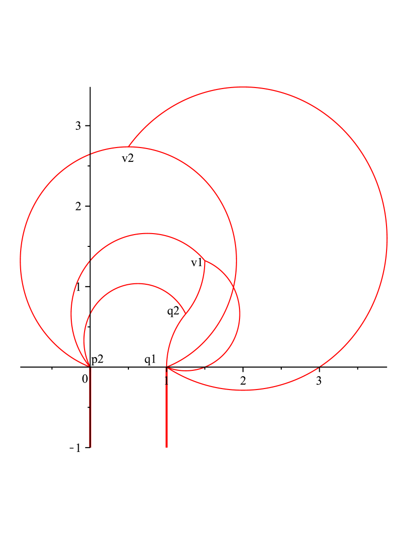
Figure 14. The projections of the faces of $T_{1}$

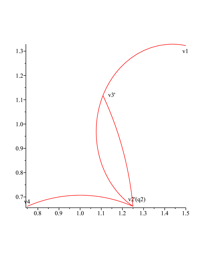
Figure 15. The projections $\Pi(F(p_{1},q_{2},v_{4}))$ is the curve $v_{4}q_{2}$, and $\Pi(F(q_{2},v^{\prime}_{2},v^{\prime}_{3}))$ is the region bounded by the two curves connecting $v^{\prime}_{2}$ and $v^{\prime}_{3}$.

7.2. Proof of Lemma 15:

As in the proof of the above lemma, we first consider the projections of the faces given in Figure 16:

• $\Pi(F(p_{1},p_{2},q_{2}))$: It is the union of the circle segment $p_{2}q_{2}$ and the negative half y-axis which is the projection of the disc part;

• $\Pi(F(p_{1},p_{2},q_{3}))$: It is the union of the circle segment $p_{2}q_{3}$ and the negative half y-axis;

• $\Pi(F(p_{1},q_{2},q_{3}))$: It is the triangle $(v_{4},q_{2},q_{3})$;

• $\Pi(F(p_{2},q_{2},q_{3}))$: It is the union of $\Pi(F(p_{2},v_{5},q_{3}))$, $\Pi(F(v_{6},q_{2},q_{3}))$ and $\Pi(F(q_{2},v_{5},v_{6}))$ which is the union of (circle) curves from the point $q_{2}$ to the (circle) curve $v_{5}v_{6}$.

The intersections of each pair of faces are easily obtained except

$$F(p_{1},q_{2},q_{3})\bigcap F(p_{2},q_{2},q_{3})=[q_{2},q_{3}]$$

and

$$F(p_{2},q_{2},q_{3})\bigcap F(p_{2},q_{2},p_{1})=[p_{2},q_{2}].$$

The first one can be obtained by considering their images under $G_{3}^{-1}$. We have to show

$$\begin{split}G_{3}^{-1}(F(p_{1},q_{2},q_{3})\bigcap F(p_{2},q_{2},q_{3}))&=G_{3}^{-1}(F(p_{1},q_{2},q_{3}))\bigcap G_{3}^{-1}(F(p_{2},q_{2},q_{3}))\\ &=F(G_{3}^{-1}(p_{1}),q_{1},p_{1})\bigcap F(p_{2},q_{1},p_{1})\\ &=[q_{1},p_{1}]=G_{3}^{-1}([q_{2},q_{3}]).\end{split}$$

Let

$$p_{1}^{\prime}=G_{3}^{-1}(p_{1})=\left(-\frac{1}{4}+i\frac{\sqrt{7}}{4},\frac{\sqrt{7}}{2}\right)$$

and

$$v_{4}^{\prime}=G_{3}^{-1}(v_{4})=\left(\frac{1}{2}+i\frac{\sqrt{7}}{2},0\right).$$

It suffice to show that

$$F(v_{4}^{\prime},q_{1},p_{1})\bigcap F(q_{1},v_{2},p_{1})=[q_{1},p_{1}],$$

since the other two sub-faces $F(p_{1},v_{4},q_{2})$ and $F(p_{1},v_{4},q_{3})$ of $F(p_{1},q_{2},q_{3})$ do not intersect the face $F(p_{2},q_{2},q_{3})$. This can be verified by analyzing their projections in Figure 17, where the projections of $F(v_{4}^{\prime},q_{1},p_{1})$ lie in the region between the straight line and the circle segment with the same endpoints $v_{4}^{\prime}$ and $q_{1}$.

To prove

$$F(p_{2},q_{2},q_{3})\bigcap F(p_{2},q_{2},p_{1})=[p_{2},q_{2}],$$

is equivalent to show

$$\begin{split}G_{3}^{-1}(F(p_{2},q_{2},q_{3}))\bigcap G_{3}^{-1}(F(p_{2},q_{2},p_{1}))&=F(p_{2},q_{1},p_{1})\bigcap F(p_{2},q_{1},p_{1}^{\prime})\\ &=[p_{2},q_{1}].\end{split}$$

The result is clear analysing the projections in Figure 17, since the projection of $F(p_{2},q_{1},p_{1}^{\prime})$ lies in the triangle $(p_{1}^{\prime},p_{2},q_{1})$.

At last, we have to mention that the intersection of $F(p_{1},p_{2},q_{2})$ and $F(p_{1},p_{2},q_{3})$ is a disc, not only an edge ($T_{2}$ is a generalized tetrahedron).

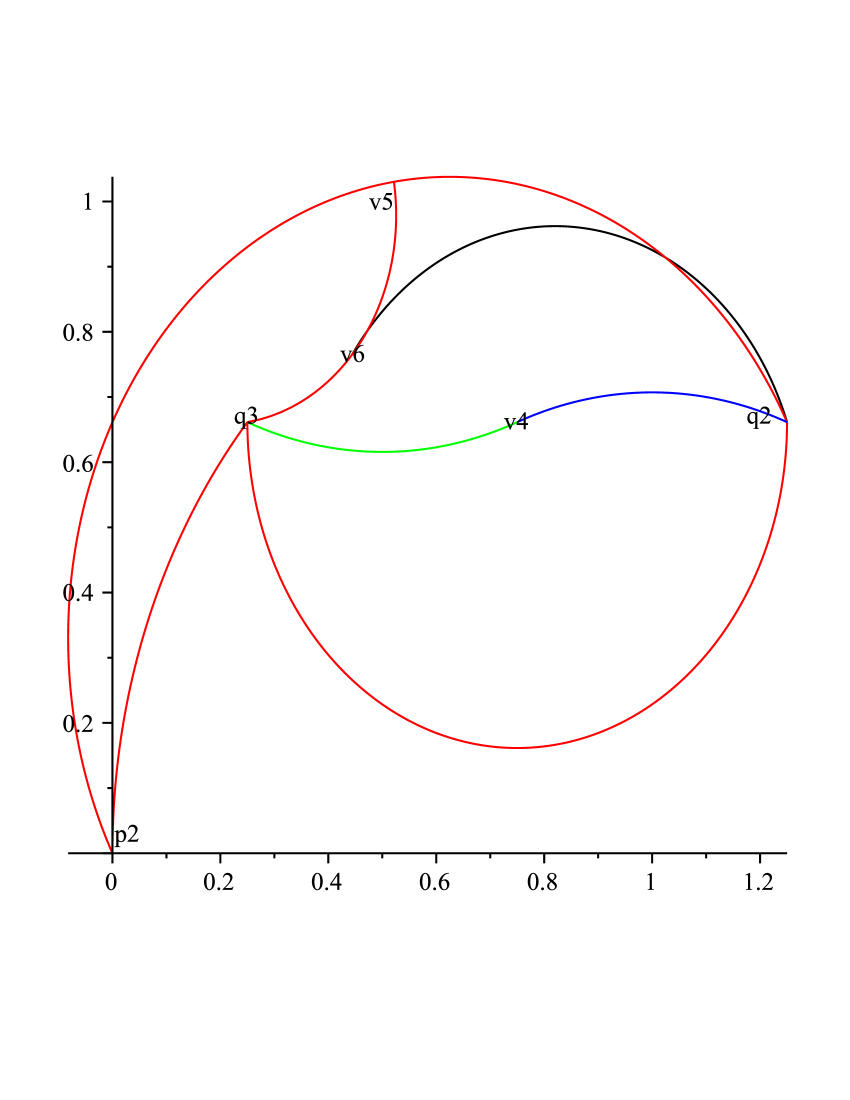
Figure 16. The projections of the faces of $T_{2}$

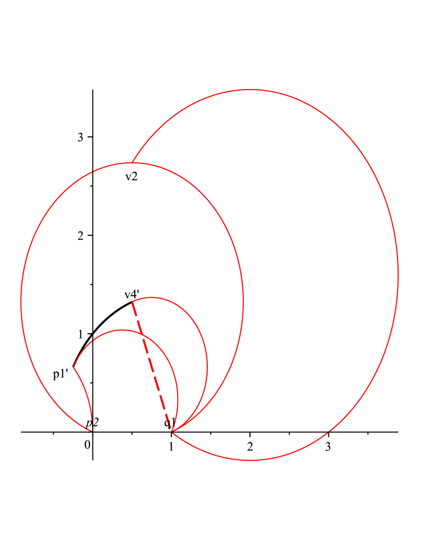
Figure 17. The projections of the faces $F(p_{1}^{\prime},q_{1},p_{1})$, $F(p_{2},q_{1},p_{1})$ and $F(p_{2},q_{1},p_{1}^{\prime})$.

7.3. Proof of Lemma 16:

According to the projections of the faces of the two tetrahedra given in Figure 18, we only need to prove the following cases in detail.

• $F(p_{1},q_{1},q_{2})\bigcap F(p_{1},q_{2},q_{3})=[p_{1},q_{2}]$. Recall that the face $F(p_{1},q_{2},q_{3})$ has three parts. It is easy to see

  $$F(p_{1},q_{1},q_{2})\bigcap F(p_{1},q_{2},v_{4})=[p_{1},q_{2}]$$

  and

  $$F(p_{1},q_{1},q_{2})\bigcap F(p_{1},v_{4},q_{3})=p_{1}.$$

  Therefore, it is suffice to show

  $$F(v_{4},q_{2},q_{3})\bigcap F(q_{1},q_{2},p_{1})=q_{2},$$

  which follows by comparing the height functions of the two faces. From their projections, we only need to compare the height of the parts where they have intersected projections, i.e. the segment $[v_{7},q_{2}]\subset[q_{1},q_{2}]$ where $v_{7}=\left(\frac{33}{32}+i\frac{3\sqrt{7}}{32},\frac{5\sqrt{7}}{8}\right)$. More precisely, write the x and y coordinates of

  $$[v_{7},q_{2}]=\left(2+e^{i\theta},\sqrt{7}-4\sin(\theta)\right)$$

  where

  $$\theta\in\left[\pi-\arcsin\left(\frac{\sqrt{7}}{4}\right),\pi-\arcsin\left(\frac{3\sqrt{7}}{32}\right)\right]$$

  into the parametrization of the face

  $$F(v_{4},q_{2},q_{3})=\left\{\begin{array}[]{ll}(x-x_{0})^{2}+(y-y_{0})^{2}=1/2\\ t=t_{0}+2(y_{0}x-x_{0}y)\end{array}\right.$$

  where

  $$\left\{\begin{array}[]{ll}x_{0}=\left(\cos(\varphi)+\sqrt{7}\sin(\varphi)+3\right)/4\\ y_{0}=\left(-\sqrt{7}\cos(\varphi)+\sin(\varphi)+\sqrt{7}\right)/4\\ t_{0}=\left(\sqrt{7}\cos(\varphi)+\sin(\varphi)\right)/2\end{array}\right.$$

  with $\varphi\in[\pi,2\pi]$, we can get the height function $t_{1}=t_{1}(\theta)$ as a function of $\theta$. Let $t_{2}=\sqrt{7}-4\sin(\theta)$, then we can compare these two height functions (see Figure 19) so that the height of $[v_{7},q_{2}]$ is bigger than that in $F(v_{4},q_{2},q_{3})$. This implies that $F(v_{4},q_{2},q_{3})$ and $F(q_{1},q_{2},p_{1})$ only intersect at the point $q_{2}$.

• $F(p_{2},q_{1},q_{2})\bigcap F(p_{2},q_{2},q_{3})=[p_{2},q_{2}]$.

• $F(p_{2},q_{1},q_{2})\bigcap F(p_{1},q_{2},q_{3})=q_{2}$.

The last two can be proved by a similar argument as in the proof of Lemma 14 and Lemma 15. More precisely, we consider their images under the action of $G_{2}$. Recall that

$$G_{2}(F(p_{2},q_{1},q_{2}))=F(p_{1},q_{2},q_{3})$$

and $v_{1}=G_{2}(p_{1})$. Let $v^{\prime}_{4}=G_{2}(q_{3})$, then

$$G_{2}(F(p_{1},q_{2},q_{3}))=F(v_{1},q_{3},v_{4}^{\prime})$$

and

$$G_{2}(F(p_{2},q_{2},q_{3}))=F(p_{1},q_{3},v_{4}^{\prime}).$$

Recall that each of these faces has three parts, according to the projected view in Figure 18 we only need to check the intersections of their subfaces

$$F(p_{2},v_{1},q_{2})\bigcap F(v_{5},v_{6},q_{2})=[v_{5},q_{2}]$$

and

$$F(v_{1},q_{1},q_{2})\bigcap F(v_{4},q_{2},q_{3})=q_{2}.$$

These can be proved by analyzing the projections of their images by $G_{2}$ in Figure 20. Precisely, let

$$v_{5}^{\prime}=G_{2}(v_{5})=\left(\frac{1}{4}+i\frac{\sqrt{7}}{4},\frac{\sqrt{2}}{8+2\sqrt{14}}\right),$$

$$v_{6}^{\prime}=G_{2}(v_{6})=\left(\frac{8-\sqrt{14}}{32+2\sqrt{14}}+i\frac{5\sqrt{2}+14\sqrt{7}}{32+2\sqrt{14}},-\frac{5\sqrt{2}+6\sqrt{7}}{32+2\sqrt{14}}\right)$$

and recall that $p_{2}=G_{2}(v_{4})$. Then their projections are:

• $\Pi(F(p_{1},q_{2},q_{3}))$ is the triangle $(v_{4},q_{2},q_{3})$;

• $\Pi(F(p_{2},q_{3},v_{4}^{\prime}))$ is the union of (circle) curves from the curve $p_{2}q_{3}$ to the point $v^{\prime}_{4}$. This projection is more complicated but lies outside the triangle $(v_{4},q_{2},q_{3})$;

• $\Pi(F(q_{3},v_{5}^{\prime},v_{6}^{\prime}))$ is the region bounded by the two curves connecting the points $v^{\prime}_{5}$ and $v^{\prime}_{6}$.

Observe that the points $v^{\prime}_{5}$ and $q_{3}$ denote the same points on the z-plane.

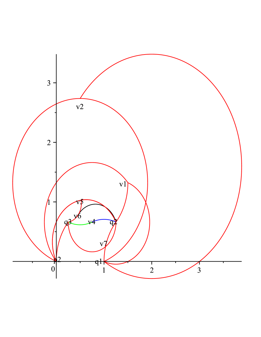
Figure 18. The projection of the subfaces of $T_{1}$ and $T_{2}$

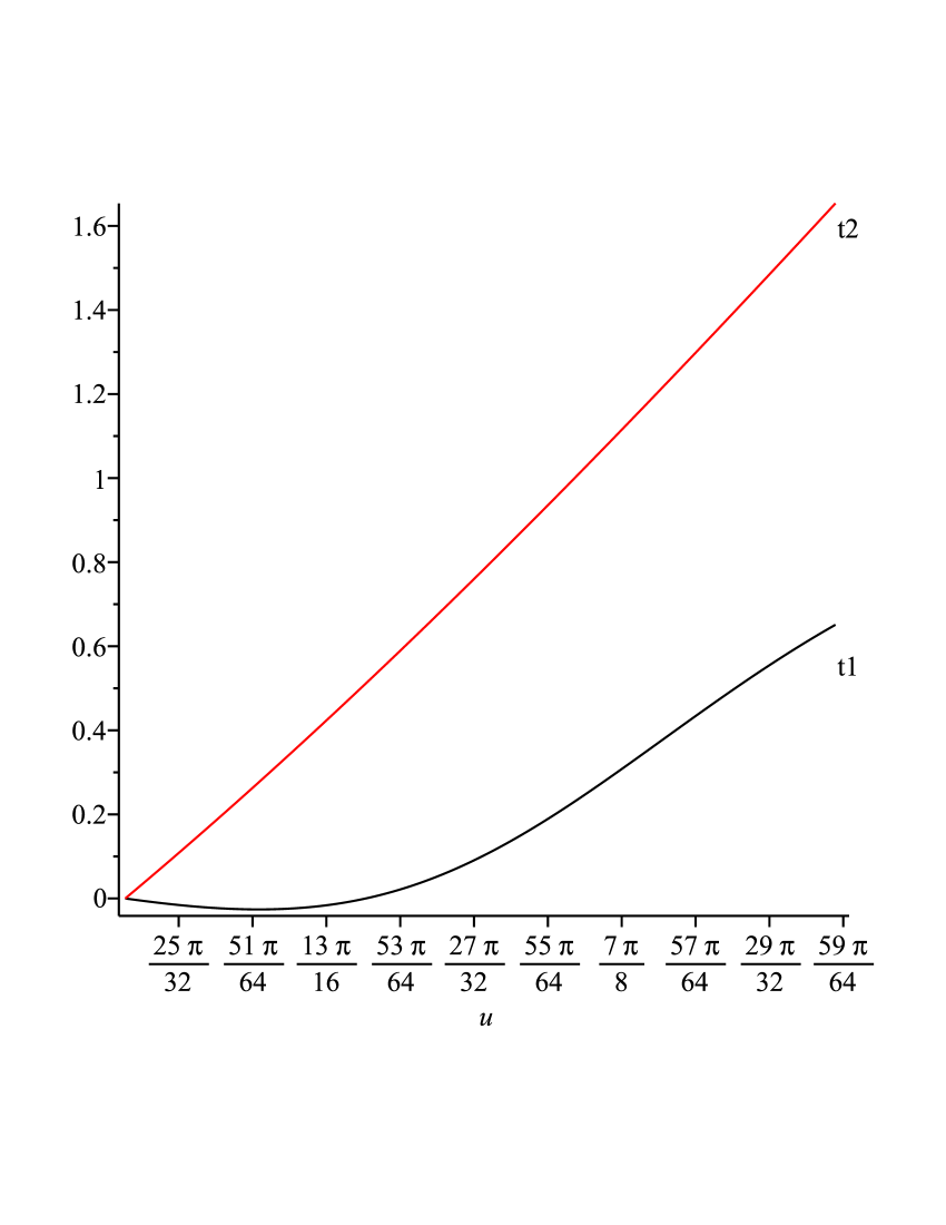
Figure 19. The height comparison, where $t_{1},t_{2}$ denote the height in $[v_{7},q_{2}]$ and $F(v_{4},q_{2},q_{3})$ respectively.

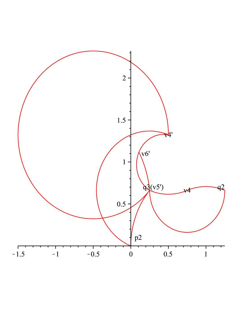
Figure 20. Projections of $F(p_{1},q_{2},q_{3})$, $F(p_{2},q_{3},v_{4}^{\prime})$ and $F(q_{3},v_{5}^{\prime},v_{6}^{\prime}).$

References

• [1] D. Burns, S. Shnider, Spherical Hypersurfaces in Complex Manifolds, Invent. Math. 33 (1976).
• [2] E. Cartan, Sur le groupe de la géométrie hypersphérique, Comm. Math. Helv. 4 (1932) 158-171.
• [3] M. Deraux, E. Falbel, The complex hyperbolic geometry of the figure eight knot. Preprint 2013.
• [4] E. Falbel, A spherical CR structure on the complement of the figure eight knot with discrete holonomy, J. Diff. G. 79 (2008), 69-110.
• [5] E. Falbel, J. Parker, The geometry of the Eisenstein-Picard modular group. Duke Math. J. 131 (2006), no. 2, 249-289.
• [6] W. M. Goldman, Complex hyperbolic geometry, Oxford Mathematical Monographs, Oxford Science Publications, The Clarendon Press, Oxford University Press, New York, 1999.
• [7] H. Jacobowitz, An introduction to CR structures. Mathematical Surveys and Monographs, 32. American Mathematical Society, Providence, RI, 1990.
• [8] J.-P. Otal, Le théorème d’hyperbolisation pour les variétés fibrées de dimension 3. Astérisque 235 (1996).
• [9] J. Parker, P. Will, A Family of Spherical CR Structures on the Whitehead Link Complement. In preparation.
• [10] A. Reid, private communication.
• [11] R. E. Schwartz, Spherical CR geometry and Dehn surgery. Annals of Mathematics Studies, 165. Princeton University Press, Princeton, NJ, (2007).
• [12] T. Zhao, Generators for the Euclidean Picard Modular Groups, Transactions of the Amer. Math. Soc. 364 (2012), 3241-3263.