Lipschitz Equivalence Class, Ideal Class and the Gauss Class Number Problem

Abstract.

Classifying fractals under bi-Lipschitz mappings in fractal geometry just as important as classifying topology spaces under homeomorphisms in topology. This paper concerns the Lipschitz equivalence of totally disconnected self-similar sets in $\mathbb{R}^{d}$ satisfying the OSC and with commensurable ratios. We obtain the complete Lipschitz invariants for such self-similar sets. The key invariant we found is an ideal related to the IFS. This discovery establishes a one-to-one correspondence between the Lipschitz equivalence classes of self-similar sets and the ideal classes in a related ring. Accordingly, two self-similar sets $A$ and $B$ with the same dimension and ratio root are Lipschitz equivalent if and only if their ideals $I_{A}$ and $I_{B}$ are equivalent, i.e., $aI_{A}=bI_{B}$ for some elements $a$ and $b$ in the related ring $R$. This result reveals an interesting relationship between the Lipschitz class number problem and the Gauss class number one problem for real quadratic fields, which was proposed by Gauss in 1801 but still remains a open question today. Our result implies that the development on the Lipschitz class number problem may lead to deeper understanding of the Gauss class number problem.

By the Jordan-Zassenhaus Theorem in algebraic number theory on the finiteness of ideal classes, we further prove a finiteness result about the Lipschitz equivalence classes under the commensurable condition. This result says that the geometrical structures of such self-similar sets are essentially finite in view of Lipschitz equivalence, although the OSC allows small copies of the self-similar sets touch in infinite geometric manners. In other words, the above finiteness result describe the open set condition in terms of Lipschitz equivalence.

By contrast, we also study the non-commensurable case. It turns out that the difference between the commensurable case and the non-commensurable case is essential. In fact, we consider the family of self-similar sets under the same restrictions only dropping the commensurable condition, and then find that there may exist infinitely many Lipschitz equivalent classes.

The simplest case of our result is that the related ring is a principal ideal domain. Then the class number is one, there is only one Lipschitz equivalence class, all self-similar sets in this class are Lipschitz equivalent to a symbolic metric space. For example, the ring $\mathbb{Z}[1/N]$ is a principal ideal domain for positive integer $N\geq 2$, then the above result implies: suppose $A$ and $B$ are totally disconnected self-similar sets satisfying the open set condition, if both $A$ and $B$ are generated by $N$ contracting similarities with the same ratio $r$, then $A$ and $B$ are Lipschitz equivalent. This very special corollary of our main result generalizes many known results on the Lipschitz equivalence of self-similar sets.

1. Introduction

1.1. Background

Two metric spaces $(X_{1},\operatorname{d}_{1})$ and $(X_{2},\operatorname{d}_{2})$ are said to be Lipschitz equivalent, denoted by $X_{1}\simeq X_{2}$, if there is a bijection $f\colon X_{1}\to X_{2}$ which is bi-Lipschitz, i.e., there exists a constant $L\geq 1$ such that

$$L^{-1}\operatorname{d}_{1}(x,y)\leq\operatorname{d}_{2}\bigl{(}f(x),f(y)\bigr{)}\leq L\operatorname{d}_{1}(x,y)\quad\text{for all $x,y\in X_{1}$}.$$

Roughly speaking, the spaces $X_{1}$ and $X_{2}$ are “almost the same” from the viewpoint of metric.

Two Lipschitz equivalent fractals can be considered as having the same geometrical structure since many important geometrical properties are invariant under the bi-Lipschitz mappings, such as

• fractal dimensions: Hausdorff dimension, packing dimension, etc;

• properties of measures: doubling, Ahlfors-David regularity, etc;

• metric properties: uniform perfectness, uniform disconnectedness, etc.

By contrast, Gromov pointed out in [21] that “isometry” leads to a poor and rather boring category and “continuity” takes us out of geometry to the realm of pure topology. So Lipschitz equivalence is suitable for the study of fractal geometry of sets. Classifying fractals under bi-Lipschitz mappings in fractal geometry just as important as classifying topology spaces under homeomorphisms in topology.

Another interesting motivation of studying Lipschitz equivalence of fractals comes from geometry group theory (see [5, 17]). For example, Farb and Mosher [17] established a quasi-isometry (in Gromov’s sense) from the group

$$\mathbf{BS}(1,n)=\langle a,b\,|\,aba=b^{n}\rangle$$

to some space with its upper boundary $C_{n}$ being a self-similar fractal. Then they proved that $\mathbf{BS}(1,n)$ and $\mathbf{BS}(1,m)$ are quasi-isometric if and only if two self-similar fractals $C_{n}$ and $C_{m}$ are Lipschitz equivalent. In the appendix of [17], Cooper obtained that $C_{n}\simeq C_{m}$ if and only if $\log m/\log n\in\mathbb{Q}$.

In general it is very difficult to determine whether two fractals are Lipschitz equivalent or not. Indeed, there is little known about the Lipschitz equivalence of fractals, even for the most familiar fractals—self similar sets in Euclidean spaces.

This paper concerns the Lipschitz equivalence of totally disconnected self-similar sets in $\mathbb{R}^{d}$ satisfying the OSC and with commensurable ratios (Definition 1.2). We obtain the complete Lipschitz invariants for such self-similar sets (Theorem 1.1). This is the first general result on the Lipschitz equivalence of self-similar sets with overlaps. The key invariant we found is an ideal related to the IFS (Definition 1.4). This discovery establishes the connection between Lipschitz equivalence class of self-similar sets and ideal class in algebraic number theory. (See, e.g., [25, 34] for detailed introduction of algebraic number theory).

Definition 1.1 (ideal class).

Two nonzero ideals $I$ and $J$ of an integral domain $R$ is said to be in the same class if $aI=bJ$ for some $a,b\in R$. The corresponding equivalence classes is called the ideal classes of $R$. The class number of $R$, denoted by $h(R)$, is defined to be the number of ideal classes.

Historically, ideal theory was developed in the investigation of Fermat’s Last Theorem. In 1844, Kummer proved Fermat’s Last Theorem for every odd prime number $p\leq 19$, based on the fact that the ring $\mathbb{Z}[e^{2\pi i/p}]$ is a unique factorization domain for such $p$. This is equivalent to $\mathbb{Z}[e^{2\pi i/p}]$ has class number $h_{p}=1$. But $h_{p}>1$ for every odd prime number $p\geq 23$, and so this proof failed for such cases. To settle this problem, in 1847, Kummer introduced “ideal numbers” to recover a form of unique factorization for the ring $\mathbb{Z}[e^{2\pi i/p}]$. As a result, Kummer can prove Fermat’s Last Theorem for all regular prime numbers $p$, which are the prime numbers such that $p\nmid h_{p}$ (all odd prime numbers less than $100$ are regular except for $37,59,67$). Kummer’s idea of “ideal number” was further developed by Dedekind, who established the modern theory of ideal in Algebra.

The study of ideal classes goes back to Lagrange and Gauss, before Kummer and Dedekind’s work on ideal. In 1773, Lagrange developed a general theory to handle the problem of when an integer $m$ is representable by a given binary quadratic form

$$m=ax^{2}+bxy+cy^{2},$$

where $a$, $b$ and $c$ are fixed integers with $\gcd(a,b,c)=1$. Some special cases of this problem had been studied by Fermat and Euler. Lagrange defined two quadratic forms $ax^{2}+bxy+cy^{2}$ and $AX^{2}+BXY+CY^{2}$ to be equivalent if there exists an invertible integral linear change of variables

$$\begin{pmatrix}x\\ y\\ \end{pmatrix}=\begin{pmatrix}\alpha&\beta\\ \gamma&\delta\\ \end{pmatrix}\begin{pmatrix}X\\ Y\\ \end{pmatrix},\quad\text{where $\alpha,\beta,\gamma,\delta\in\mathbb{Z}$ with}\ \begin{vmatrix}\alpha&\beta\\ \gamma&\delta\\ \end{vmatrix}=\pm 1,$$

that transforms $ax^{2}+bxy+cy^{2}$ to $AX^{2}+BXY+CY^{2}$. Note that equivalent forms have the same discriminant $D=b^{2}-4ac$, and more important that equivalent forms represent the same set of integers. Let $h(D)$ denote the number of equivalence classes of binary quadratic forms with discriminant $D$. In Disquisitiones Arithmeticae published in 1801, Gauss further studied this problem and proved that $h(D)$ is finite for every value $D$. Moreover, Gauss put forward his famous class number problems (see Section 1.3). The relationship between the equivalence class of quadratic forms and ideal class is that, for every negative square free integer $D$, the equivalence classes of binary quadratic forms with discriminant $D$ correspond one-to-one to the ideal classes of the ring $\mathcal{O}_{D}$, which is the ring of all algebraic integers in $\mathbb{Q}(\sqrt{D})$. In other words, $h(D)$ equals the class number of $\mathcal{O}_{D}$ for every negative square free integer $D$ (see, e.g., [20, 41]).

Just like the binary quadratic forms, for some appropriate families of self-similar sets, we can establish a one-to-one correspondence between the Lipschitz equivalence classes and the ideal classes of a related ring (Theorem 1.2 and 1.3).

1.2. Main results

For convenience, we recall some basic notions of self-similar sets, see [15, 16, 23] for more details. Let $\mathcal{S}=\{S_{1},S_{2},\dots,S_{N}\}$ be an iterated functions system (IFS) on a complete metric space $(X,\operatorname{d})$ where each $S_{i}$ is a contracting similarity of ratio $r_{i}\in(0,1)$, i.e., $\operatorname{d}\bigl{(}S_{i}(x),S_{i}(y)\bigr{)}=r_{i}\operatorname{d}(x,y)$. The self-similar set generated by the IFS $\mathcal{S}$ is the unique nonempty compact set $E_{\mathcal{S}}\subset X$ such that $E_{\mathcal{S}}=\bigcup_{i=1}^{N}S_{i}(E_{\mathcal{S}})$. We say that the IFS $\mathcal{S}$ satisfies the strong separation condition (SSC) if the sets $\{S_{i}(E_{\mathcal{S}})\}$ are pairwise disjoint. The IFS $\mathcal{S}$ satisfies the open set condition (OSC) if there exists a nonempty bounded open set $O$ such that the sets $S_{i}(O)$ are disjoint and contained in $O$. If furthermore $O\cap E_{\mathcal{S}}\neq\emptyset$, we say that the IFS $\mathcal{S}$ satisfies the strong open set condition (SOSC). Obviously, we have

$$\text{SSC}\Rightarrow\text{SOSC}\Rightarrow\text{OSC}.$$

For IFSs on Euclidean spaces, Hutchinson [23], Bandt and Graf [2] and Schief [39] proved that $\operatorname{\dim_{H}}E_{\mathcal{S}}$ equals the similarity dimension $s$ (the unique positive solution of $\sum_{i=1}^{N}r_{i}^{s}=1$) if $\mathcal{S}$ satisfies the OSC, and that

$$\text{SOSC}\Leftrightarrow\text{OSC}\Leftrightarrow\mathcal{H}^{s}(E_{\mathcal{S}})>0.$$

Here $\mathcal{H}^{s}$ denotes the $s$-dimensional Hausdorff measure.

Definition 1.2 (commensurable).

The ratios $r_{1},\dots,r_{N}$ of the IFS $\mathcal{S}$ are said to be commensurable if the multiplicative group generated by $\{r_{1},\dots,r_{N}\}$ can be generated by a single number $r_{\mathcal{S}}\in(0,1)$. In other words, $r_{i}=r_{\mathcal{S}}^{\lambda_{i}}$ with $\lambda_{i}\in\mathbb{N}$ for each $i$ and $\gcd(\lambda_{1},\dots,\lambda_{N})=1$. We call $r_{\mathcal{S}}$ the ratio root of $\mathcal{S}$.

Remark 1.1.

The ratios $r_{1},\dots,r_{N}$ are commensurable if and only if $\log r_{i}/\log r_{j}\in\mathbb{Q}$ for $1\leq i,j\leq N$.

We say the IFS $\mathcal{S}$ satisfies the TDC, denoted by $\mathcal{S}\in\mathrm{TDC}$, if the corresponding self-similar set $E_{\mathcal{S}}$ is totally disconnected. Write

$$\mathrm{OSC^{E}_{1}}=\bigl{\{}\mathcal{S}\colon\text{$\mathcal{S}$ is an IFS on a Euclidean space}\\ \text{satisfying the OSC and with commensurable ratios}\bigr{\}}.$$

In this paper, we introduce an ideal related to $\mathcal{S}\in\mathrm{TDC}\cap\mathrm{OSC^{E}_{1}}$ which turns out to be a very important Lipschitz invariant. For an IFS $\mathcal{S}=\{S_{1},\dots,S_{N}\}$ satisfying the OSC, the natural measure $\mu_{\mathcal{S}}$ of $\mathcal{S}$ is defined to be the normalized $s$-dimensional Hausdorff measure restricted to $E_{\mathcal{S}}$, where $s=\operatorname{\dim_{H}}E_{\mathcal{S}}$, i.e., $\mu_{\mathcal{S}}=\mathcal{H}^{s}|_{E_{\mathcal{S}}}/\mathcal{H}^{s}(E_{\mathcal{S}})$. Note that $\mu_{\mathcal{S}}$ is the unique Borel probability measure such that

$$\mu_{\mathcal{S}}(A)=\sum_{i=1}^{N}r_{i}^{s}\mu_{\mathcal{S}}\bigl{(}S_{i}^{-1}(A)\bigr{)}\quad\text{for all Borel sets~{}$A$}.$$

For $\mathcal{S}\in\mathrm{OSC^{E}_{1}}$, we call $p_{\mathcal{S}}=r_{\mathcal{S}}^{s}$ the measure root of $\mathcal{S}$ (see Remark 5.2). It follows from $\sum_{i=1}^{N}r_{i}^{s}=1$ and $\log r_{i}/\log r_{\mathcal{S}}$ is a positive integer that $p_{\mathcal{S}}^{-1}$ is an algebraic integer. Let

$$\mathbb{Z}[p_{\mathcal{S}}]=\bigl{\{}P(p_{\mathcal{S}})\colon\text{$P$ is a polynomial with integer coefficients}\bigr{\}}$$

be the ring generated by $p_{\mathcal{S}}$ over the integer set $\mathbb{Z}$.

Definition 1.3 (interior separated set).

Suppose that $\mathcal{S}\in\mathrm{TDC}\cap\mathrm{OSC^{E}_{1}}$. A compact set $F\subset E_{\mathcal{S}}$ is called an interior separated set of $E_{\mathcal{S}}$ if $E_{\mathcal{S}}\setminus F$ is also compact and $F\subset O$ for some open set $O$ satisfying the OSC.

We remark that $\mu_{\mathcal{S}}(F)\in\mathbb{Z}[p_{\mathcal{S}}]$ for every interior separated set $F$.

Definition 1.4 (ideal of IFS).

Suppose that $\mathcal{S}\in\mathrm{TDC}\cap\mathrm{OSC^{E}_{1}}$. The ideal of $\mathcal{S}$, denoted by $I_{\mathcal{S}}$, is defined to be the ideal of $\mathbb{Z}[p_{\mathcal{S}}]$ generated by

$$\bigl{\{}\mu_{\mathcal{S}}(F)\colon\text{$F$ is an interior separated set of~{}$E_{\mathcal{S}}$}\bigr{\}}.$$

Remark 1.2.

It is worth noting that the ideal $I_{\mathcal{S}}$ depends not only on the algebraic properties of ratios, but also on the geometrical structure of the self-similar set $E_{\mathcal{S}}$.

Remark 1.3.

At first sight it seems that we need find all open sets which satisfy the SOSC if we want to determine the ideal of an IFS. Fortunately, one such open set is enough, see Remark 5.6 in Section 5.3.

Example 1.1.

We have $I_{\mathcal{S}}=\mathbb{Z}[p_{\mathcal{S}}]$ when $\mathcal{S}$ satisfies the SSC. Indeed, the open set $O=\{x\colon\operatorname{dist}(x,E_{\mathcal{S}})<\varepsilon\}$ satisfies the OSC for $\varepsilon$ small enough. And so $E_{\mathcal{S}}\subset O$ is an interior separated set. Therefore $1=\mu_{\mathcal{S}}(E_{\mathcal{S}})\in I_{\mathcal{S}}$ and $I_{\mathcal{S}}=\mathbb{Z}[p_{\mathcal{S}}]$.

Our main result gives the complete Lipschitz invariants of self-similar sets generated by IFSs in $\mathrm{TDC}\cap\mathrm{OSC^{E}_{1}}$. This is the first general result on the Lipschitz equivalence of self-similar sets with overlaps.

Theorem 1.1.

Suppose that $\mathcal{S},\mathcal{T}\in\mathrm{TDC}\cap\mathrm{OSC^{E}_{1}}$, then $E_{\mathcal{S}}\simeq E_{\mathcal{T}}$ if and only if

1. $\operatorname{\dim_{H}}E_{\mathcal{S}}=\operatorname{\dim_{H}}E_{\mathcal{T}}$;

2. $\log r_{\mathcal{S}}/\log r_{\mathcal{T}}\in\mathbb{Q}$;

3. $I_{\mathcal{S}}=aI_{\mathcal{T}}$ for some $a\in\mathbb{R}$.

Remark 1.4.

We emphasize that, in Theorem 1.1, the two IFSs $\mathcal{S}$ and $\mathcal{T}$ are allowed to be defined on Euclidean spaces of different dimensions. For example, the IFS $\mathcal{S}$ in Example 1.3 is defined on $\mathbb{R}^{1}$ and the IFS $\mathcal{S}$ in Example 4.2 is defined on $\mathbb{R}^{2}$. By Theorem 1.1, the two corresponding self-similar sets are Lipschitz equivalent, see Figure 1 and 6.

Theorem 1.1 offers much deep insight into the geometrical structure of self-similar sets generated by IFSs in $\mathrm{TDC}\cap\mathrm{OSC^{E}_{1}}$. To make this more clear, we shall consider a family of self-similar sets with the same ratio root to eliminate the influence of ratios. Let $\mathrm{OSC^{E}_{1}}(p,r)$ denote the set consisting of all IFS $\mathcal{S}\in\mathrm{OSC^{E}_{1}}$ with $p_{\mathcal{S}}=p$ and $r_{\mathcal{S}}=r$. Given $\mathcal{S},\mathcal{T}\in\mathrm{TDC}\cap\mathrm{OSC^{E}_{1}}(p,r)$, we have $\operatorname{\dim_{H}}E_{\mathcal{S}}=\operatorname{\dim_{H}}E_{\mathcal{T}}=\log p/\log r$ and $r_{\mathcal{S}}=r_{\mathcal{T}}=r$. Therefore, Conditions (i) and (ii) in Theorem 1.1 are fulfilled and the ideals $I_{\mathcal{S}}$ and $I_{\mathcal{T}}$ belong to the same ring $\mathbb{Z}[p]$. Consequently, we have

Theorem 1.2.

Suppose that $\mathcal{S},\mathcal{T}\in\mathrm{TDC}\cap\mathrm{OSC^{E}_{1}}(p,r)$, then the two self-similar sets $E_{\mathcal{S}}$ and $E_{\mathcal{T}}$ are Lipschitz equivalent if and only if their ideals $I_{\mathcal{S}}$ and $I_{\mathcal{T}}$ belong to the same ideal class of $\mathbb{Z}[p]$.

Roughly speaking, Theorem 1.2 tells us that different Lipschitz equivalence classes correspond to different ideal classes, see Example 1.3. It is natural to ask whether the correspondence induced by Theorem 1.2 is one-to-one. Our next result gives an affirm answer to this question. We define the number of Lipschitz equivalence classes of self-similar sets generated by IFSs in $\mathrm{TDC}\cap\mathrm{OSC^{E}_{1}}(p,r)$ to be the Lipschitz class number of $\mathrm{TDC}\cap\mathrm{OSC^{E}_{1}}(p,r)$, denoted by $h_{\mathrm{L}}(p,r)$.

Theorem 1.3.

Suppose that $\mathrm{TDC}\cap\mathrm{OSC^{E}_{1}}(p,r)\neq\emptyset$. Then the Lipschitz equivalent classes of self-similar sets generated by IFSs in $\mathrm{TDC}\cap\mathrm{OSC^{E}_{1}}(p,r)$ correspond one-to-one to the ideal classes of $\mathbb{Z}[p]$. This means $h_{\mathrm{L}}(p,r)=h(\mathbb{Z}[p])$. Moveover, the Lipschitz class number $h_{\mathrm{L}}(p,r)$ is finite for every pair $p,r$.

The most significance of Theorem 1.3 is the one-to-one correspondence between the Lipschitz equivalence classes and the ideal classes. We will further discuss this point in next subsection.

It is also worth noting that the finiteness result about the Lipschitz equivalence classes gives some interesting information about the OSC. For self-similar fractals, the OSC is a generally accepted separation condition, but it is too complicated to describe completely in geometry. For example, the OSC allows the small copies of self-similar set touch in infinitely many geometric manners. However, the finiteness result in Theorem 1.3 says that the touching manners is essentially finite in view of Lipschitz equivalence. In other words, this finiteness result describes the open set condition in term of Lipschitz equivalence.

We present two examples to illustrate Theorem 1.3. For positive square free integer $D$, let $\mathcal{O}_{D}$ be the ring of all algebraic integers in the field $\mathbb{Q}(\sqrt{D})$. We know from algebraic number theory that

$$\mathcal{O}_{D}=\begin{cases}\mathbb{Z}[\sqrt{D}],&\text{if $D\equiv 2$ or $3\pmod{4}$};\\ \mathbb{Z}[\frac{1+\sqrt{D}}{2}],&\text{if $D\equiv 1\pmod{4}$};\end{cases}$$

and

$$h(\mathcal{O}_{D})=1\quad \text{for $D=2,3,5,6,7,11,13,14,17,19,21,22,23,29,\dots$};$$

$$h(\mathcal{O}_{D})=2\quad \text{for $D=10,15,26,30,34,35,39,42,51,55,58,65,\dots$}.$$

For more square free $D>0$ with $h(\mathcal{O}_{D})=1$ or $2$, see [31, 32]. Using the above facts about the class number of $\mathcal{O}_{D}$, we give the following two examples.

Example 1.2.

Let $p=(\sqrt{5}-1)/2$, then $p^{4}+p^{3}+p=1$ and $p^{3}+2p^{2}=1$. Suppose that $\mathcal{S},\mathcal{T}\in\mathrm{TDC}\cap\mathrm{OSC^{E}_{1}}(p,r)$ with ratios $r^{4},r^{3},r$ and $r^{3},r^{2},r^{2}$, respectively, then $p_{\mathcal{S}}=p_{\mathcal{T}}=p$. Since $\mathbb{Z}[p]=\mathbb{Z}[p+1]=\mathcal{O}_{5}$ has class number one, we have $E_{\mathcal{S}}\simeq E_{\mathcal{T}}$. In this example, the relative positions of the small copies of self-similar sets $E_{\mathcal{S}}$ and $E_{\mathcal{T}}$ do not affect the Lipschitz equivalence.

The following example involves the ring $\mathcal{O}_{10}$, which has class number $2$. We consider the IFS family $\mathrm{TDC}\cap\mathrm{OSC^{E}_{1}}(p,r)$ with $p=\sqrt{10}-3$ and $r=1/10$. Theorem 1.3 says that there are two Lipschitz equivalence classes since $\mathbb{Z}[p]=\mathbb{Z}[\sqrt{10}]=\mathcal{O}_{10}$.

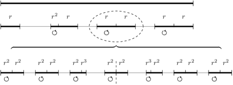
Figure 1. The structure of $E_{\mathcal{S}}$ in Example 1.3

Example 1.3.

Let $\mathcal{S}=\{S_{1},S_{2},\dots,S_{7}\}\in\mathrm{TDC}\cap\mathrm{OSC^{E}_{1}}(p,r)$, where $p=\sqrt{10}-3$, $r=1/10$ and

$$S_{1}\colon x\mapsto rx,\quad S_{2}\colon x\mapsto-r^{2}x+3r,\quad S_{3}\colon x\mapsto rx+3r,$$

$$S_{4}\colon x\mapsto-rx+6r,\quad S_{5}\colon x\mapsto rx+6r,\quad S_{6}\colon x\mapsto-rx+9r,\quad S_{7}\colon x\mapsto rx+9r.$$

See Figure 1. (In Figure 1, the symbol $\bm{\circlearrowleft}$ means that there is a minus sign in the contraction coefficient of the corresponding similarity. In geometry, this means a rotation by the angle $\pi$.) Then $p_{\mathcal{S}}=p=\sqrt{10}-3$ satisfying the equation $p^{2}+6p=1$, and Example 4.1 shows

$$I_{\mathcal{S}}=(2,p+1)=(2,\sqrt{10})=\bigl{\{}2a+b\sqrt{10}\colon a,b\in\mathbb{Z}\bigr{\}}.$$

One can check that $I_{\mathcal{S}}$ is not a principal ideal of the ring $\mathbb{Z}[p_{\mathcal{S}}]=\mathcal{O}_{10}$.

Let $\mathcal{T}\in\mathrm{TDC}\cap\mathrm{OSC^{E}_{1}}(p,r)$ satisfying the SSC with ratios $r^{2},r,r,r,r,r,r$. Then $p_{\mathcal{T}}=p=\sqrt{10}-3$, and by Example 1.1, $I_{\mathcal{T}}=\mathbb{Z}[p_{\mathcal{T}}]=\mathcal{O}_{10}$ is a principal ideal.

Theorem 1.3 implies that $E_{\mathcal{S}}\not\simeq E_{\mathcal{T}}$ and that either $E\simeq E_{\mathcal{S}}$ or $E\simeq E_{\mathcal{T}}$ for every self-similar set $E$ generated by IFS in $\mathrm{TDC}\cap\mathrm{OSC^{E}_{1}}(p,r)$. In this example, the relative positions of the small copies of self-similar sets do affect the Lipschitz equivalence.

We close this subsection with a necessary and sufficient condition for the IFS family $\mathrm{TDC}\cap\mathrm{OSC^{E}_{1}}(p,r)\neq\emptyset$.

Proposition 1.1.

The IFS family $\mathrm{TDC}\cap\mathrm{OSC^{E}_{1}}(p,r)\neq\emptyset$ if and only if $p,r\in(0,1)$ and there exist positive integers $\lambda_{1},\lambda_{2},\dots,\lambda_{N}$ with $\gcd(\lambda_{1},\dots,\lambda_{N})=1$ such that

$$p^{\lambda_{1}}+p^{\lambda_{2}}+\dots+p^{\lambda_{N}}=1.$$

Here we allow that $\lambda_{i}=\lambda_{j}$ for $i\neq j$.

1.3. Class number problem

In this subsection, we will discuss the Lipschitz class number of $\mathrm{TDC}\cap\mathrm{OSC^{E}_{1}}(p,r)$ by making use of Theorem 1.3. This problem is closely related to the famous class number problems posed by Gauss in Articles 303 and 304 of Disquisitiones Arithmeticae of 1801.

Recall that the class number of an algebraic number field is defined to be the class number of the ring of all algebraic integers in it. We state some Gauss class number problems in the modern terminology.

Gauss class number conjecture.

The number of imaginary quadratic fields $\mathbb{Q}(\sqrt{D})$ $(D<0)$ which have a given class number $n$ is finite.

This conjecture was solved by Heilbronn in 1934. Gauss further posed the following problem.

Gauss class number problem.

For small $n$, determine all $D<0$ such that the class number of $\mathbb{Q}(\sqrt{D})$ equals $n$.

Watkins [43] gave the solution for $n\leq 100$ in 2004. As a special case,

Gauss class number one problem for imaginary quadratic fields.

There are only nine imaginary quadratic fields $\mathbb{Q}(\sqrt{D})$ $(D<0)$ with class number one. They are

$$D\in\{-1,-2,-3,-7,-11,-19,-43,-67,-163\}.$$

This conjecture was solved by Baker [1] and Stark [40] independently in 1967. For the contrasting case of real quadratic fields, Gauss conjecture

Gauss class number one problem for real quadratic fields.

There are infinitely many real quadratic fields $\mathbb{Q}(\sqrt{D})$ $(D>0)$ with class number one.

This conjecture is still open. We do not even yet know whether there are infinitely many algebraic number fields (of arbitrary degree) with class number one.

Like the Gauss class number problems, we can pose the Lipschitz class number problem.

Question 1.

For a given integer $n>0$, determine all $p,r$ such that $h_{\mathrm{L}}(p,r)=n$.

Theorem 1.3 says that $h_{\mathrm{L}}(p,r)=n$ if and only if $\mathrm{TDC}\cap\mathrm{OSC^{E}_{1}}(p,r)\neq\emptyset$ (see Proposition 1.1) and $h(\mathbb{Z}[p])=n$. However, from the Gauss class number problems, we know that, in algebraic number theory, it is very difficult to determine all the algebraic numbers $p$ such that the ring $\mathbb{Z}[p]$ has a given class number $n$. In other words, it seems very hard to solve Question 1 by making use of algebraic number theory. A natural question is: can we obtain some results on Question 1 by analyzing the geometrical structure of self-similar sets directly? Such results, if obtained, might lead to deeper understanding of the Gauss class number problems. Of course, this is also very difficult. We don’t know how to do it so far.

1.4. More results on principal ideal

The simplest case of Theorem 1.3 is that the ring $\mathbb{Z}[p]$ is a principal ideal domain.

Theorem 1.4.

Suppose that $\mathcal{S},\mathcal{T}\in\mathrm{TDC}\cap\mathrm{OSC^{E}_{1}}(p,r)$. If $\mathbb{Z}[p]$ is a principal ideal domain, then $E_{\mathcal{S}}\simeq E_{\mathcal{T}}$.

Remark 1.5.

Like the SSC, in this case the relative positions of the small copies of self-similar sets do not affect the Lipschitz equivalence.

The simplest example of $\mathbb{Z}[p]$ to be a principal ideal domain is that $p=1/N$ for integers $N\geq 2$. Given $\mathcal{S}=\{S_{1},\dots,S_{N}\}\in\mathrm{TDC}\cap\mathrm{OSC^{E}_{1}}$ with the $N$ ratios are all equal to $r$, the ring related to $\mathcal{S}$ is just $\mathbb{Z}[1/N]$. This leads to the following theorem.

Theorem 1.5.

Suppose $E\subset\mathbb{R}^{d}$ and $E^{\prime}\subset\mathbb{R}^{d^{\prime}}$ are totally disconnected self-similar sets satisfying the open set condition, if both $E$ and $E^{\prime}$ are generated by $N$ contracting similarities with the same ratio $r$, then $E$ and $E^{\prime}$ are Lipschitz equivalent.

Remark 1.6.

Theorem 1.5 generalizes many known results on the Lipschitz equivalence of self-similar sets (see Section 2.4), although it is only a very special corollary of Theorem 1.3.

On the other hand, it is natural to think that a self-similar set has the simplest geometrical structure if it is Lipschitz equivalent to a self-similar set satisfying the SSC. If the set is generated by an IFS $\mathcal{S}\in\mathrm{TDC}\cap\mathrm{OSC^{E}_{1}}$, by Theorem 1.1 and Example 1.1, this is equivalent to that the ideal $I_{\mathcal{S}}$ is a principle ideal. Let $\mathrm{PI}$ denote the set of all IFS $\mathcal{S}\in\mathrm{TDC}\cap\mathrm{OSC^{E}_{1}}$ such that the ideal $I_{\mathcal{S}}$ is a principal ideal. It follows from Theorem 1.1 that

Theorem 1.6.

Suppose that $\mathcal{S},\mathcal{T}\in\mathrm{PI}$, then $E_{\mathcal{S}}\simeq E_{\mathcal{T}}$ if and only if

1. $\operatorname{\dim_{H}}E_{\mathcal{S}}=\operatorname{\dim_{H}}E_{\mathcal{T}}$;

2. $\log r_{\mathcal{S}}/\log r_{\mathcal{T}}\in\mathbb{Q}$;

3. $\mathbb{Z}[p_{\mathcal{S}}]=\mathbb{Z}[p_{\mathcal{T}}]$.

The point is that the condition $I_{\mathcal{S}}=aI_{\mathcal{T}}$ in Theorem 1.1 is equivalent to $\mathbb{Z}[p_{\mathcal{S}}]=\mathbb{Z}[p_{\mathcal{T}}]$ provided that $I_{\mathcal{S}}$ and $I_{\mathcal{T}}$ are both principle ideals. In fact, under the assumption of being principle ideal, $I_{\mathcal{S}}=aI_{\mathcal{T}}$ is equivalent to $\mathbb{Z}[p_{\mathcal{S}}]=b\mathbb{Z}[p_{\mathcal{T}}]$ for some $b\in\mathbb{R}$. Then observe that $b\in\mathbb{Z}[p_{\mathcal{S}}]$ since $1\in\mathbb{Z}[p_{\mathcal{T}}]$, and so $b\mathbb{Z}[p_{\mathcal{S}}]\subset\mathbb{Z}[p_{\mathcal{S}}]=b\mathbb{Z}[p_{\mathcal{T}}]$, i.e., $\mathbb{Z}[p_{\mathcal{S}}]\subset\mathbb{Z}[p_{\mathcal{T}}]$. By symmetry we have $\mathbb{Z}[p_{\mathcal{S}}]=\mathbb{Z}[p_{\mathcal{T}}]$. However, in general $I_{\mathcal{S}}=aI_{\mathcal{T}}$ is not equivalent to $\mathbb{Z}[p_{\mathcal{S}}]=\mathbb{Z}[p_{\mathcal{T}}]$, see Example 1.4.

Example 1.4.

Let $p_{\mathcal{S}}=\sqrt{10}-3$ be the positive solution of the equation $p_{\mathcal{S}}^{2}+6p_{\mathcal{S}}=1$ and $p_{\mathcal{T}}=37\sqrt{10}-117$ the positive solution of the equation $p_{\mathcal{T}}^{2}+234p_{\mathcal{T}}=1$. Then $\mathbb{Z}[p_{\mathcal{S}}]=\mathbb{Z}[\sqrt{10}]\neq\mathbb{Z}[p_{\mathcal{S}}]=\mathbb{Z}[37\sqrt{10}]$. Let $I_{\mathcal{S}}=I_{\mathcal{T}}=37(\sqrt{10}\mathbb{Z}+2\mathbb{Z})$. One can check that $I_{\mathcal{S}}$ is an ideal of $\mathbb{Z}[p_{\mathcal{S}}]$ and $I_{\mathcal{T}}$ is an ideal of $\mathbb{Z}[p_{\mathcal{T}}]$. Thus, $I_{\mathcal{S}}=I_{\mathcal{T}}$ but $\mathbb{Z}[p_{\mathcal{S}}]\neq\mathbb{Z}[p_{\mathcal{T}}]$.

A natural question arises:

Question 2.

For what IFS $\mathcal{S}\in\mathrm{TDC}\cap\mathrm{OSC^{E}_{1}}$, is the ideal $I_{\mathcal{S}}$ a principal ideal?

We remark that Example 1.1 says that $\mathrm{PI}$ contains all IFS $\mathcal{S}\in\mathrm{TDC}\cap\mathrm{OSC^{E}_{1}}$ satisfying the SSC. It is also obviously that $\mathcal{S}\in\mathrm{PI}$ if $\mathbb{Z}[p_{\mathcal{S}}]$ is a principle ideal domain. We further give another partial answer to Question 2. An IFS $\mathcal{S}$ on $\mathbb{R}^{d}$ is said to be orthogonal homogeneous if there is a $d\times d$ orthogonal matrix $\bm{A}$ such that each $S_{i}\in\mathcal{S}$ has the form $S_{i}\colon x\mapsto r_{i}\bm{A}x+b_{i}$ with $r_{i}\in(0,1)$. In other words, the similarities in $\mathcal{S}$ have the same orthogonal part but their ratios may be different. We say an IFS $\mathcal{S}$ satisfies the convex open set condition (COSC) if $\mathcal{S}$ satisfies the OSC with a convex open set. Let

(1.1) $$\mathscr{S}:=\Bigl{\{}\mathcal{S}\in\mathrm{TDC}\cap\mathrm{OSC^{E}_{1}}\colon\text{$\mathcal{S}$ satisfies the COSC}\\ \text{and is orthogonal homogeneous}\Bigr{\}}.$$

Theorem 1.7.

For every $\mathcal{S}\in\mathscr{S}$, we have $I_{\mathcal{S}}=\mathbb{Z}[p_{\mathcal{S}}]$. As a result, $\mathscr{S}\subset\mathrm{PI}$.

Remark 1.7.

We don’t know whether Theorem 1.7 is still true if we drop the COSC. On the other hand, Example 1.3 and 4.2 implies that the condition that $\mathcal{S}$ is orthogonal homogeneous can not be relaxed too much.

Remark 1.8.

Under the commensurable case, Theorem 1.6 and 1.7 extend the results in [38, 48] in a very general setting for IFSs on $\mathbb{R}^{d}$ ($d\geq 1$), see Section 2.4.

The paper is organized as follows. In Section 2, we review some known results about the Lipschitz equivalence of self-similar sets and present some new results on the non-commensurable case, including Theorem 2.2 and 2.3. Section 3 concerns the algebraic properties of measure root. As a result, we give the proof of Proportion 1.1. Section 4 devoted to the proof of Theorem 1.3 and 1.7. This is based on some techniques of computing the ideal of IFS, see Theorem 4.2 and 4.3. Section 5 introduces the notions of blocks decomposition, interior blocks and measure polynomials. This section also prove some basic results, such as the finiteness of the measure polynomials (Proposition 5.1) and the cardinality of boundary blocks and interior blocks (Lemma 5.7, 5.8 and 5.9). All of this are fundamental to our study. Section 6 discusses the main ideas behind the proof of Theorem 1.1, including the cylinder structure (Definition 6.3), the dense island structure (Definition 6.5), the measure linear property (Definition 6.7) and the suitable decomposition (Definition 6.8). We conclude this section with Lemma 6.3, which is the tool to construct the same cylinder structure. The proof of Theorem 1.1 is presented in Section 7 and 8. By making use of cylinder structure and dense island structure, we first prove the whole self-similar set is Lipschitz equivalent to interior blocks of it (Proposition 7.1), then deal with the Lipschitz equivalence between interior blocks of different self-similar sets (Proposition 8.1). Thus the proof of Theorem 1.1 is complete. Finally, we study the non-commensurable case and give the proofs of Theorem 2.2 and 2.3 in Section 9.

2. Geometrical structure of Self-similar Sets

2.1. About self-similar sets

Self-similar sets in Euclidean spaces are fundamental objects in fractal geometry. However, we do not know much about them.

Given an IFS $\mathcal{S}=\{S_{i}\}_{i=1}^{N}$ consisting of contracting similarities $\mathcal{S}=\{S_{i}\}_{i=1}^{N}$ on $\mathbb{R}^{d}$, Hutchinson [23] showed that there is a unique nonempty compact set $E_{\mathcal{S}}\subset\mathbb{R}^{d}$, called self-similar set, such that

$$E_{\mathcal{S}}=\bigcup_{i=1}^{N}S_{i}(E_{\mathcal{S}}).$$

Conversely, given a self-similar set $E$, it is not easy to determine all the IFSs which generate $E$, even under some reasonable additional conditions. This is why we state our results by IFSs rather than self-similar sets. This problem is rather fundamental and has some relationship with the Lipschitz equivalence problem of self-similar sets. In fact, if two IFSs generate the same self-similar set, they must satisfy the conditions necessary to the Lipschitz equivalence. It is somewhat surprising that there is little known about the generating IFSs of a given self-similar set. We refer to [12, 19] for detailed study of this problem.

Another basic problem is to determine the dimension of self-similar sets. In general this problem is very difficult. A open conjecture of Furstenberg says that $\operatorname{\dim_{H}}E_{\lambda}=1$ for any $\lambda$ irrational, where $E_{\lambda}=E_{\lambda}/3\cup(E_{\lambda}/3+\lambda/3)\cup(E_{\lambda}/3+2/3)$. Although the IFSs involved are rather sample, the conjecture remained open from 1970s until settled by Hochman [22] very recently, see also [24, 37, 42]. We know much more about the dimension of self-similar sets if some separation conditions hold. Such conditions control the overlaps between small copies of self-similar set. The OSC, which means the overlaps are small, was introduced by Moran [33]. For IFSs on Euclidean spaces, it is well known from Hutchinson [23] that if $\mathcal{S}$ satisfies the OSC, then $\operatorname{\dim_{H}}E_{\mathcal{S}}$ equals the similarity dimension $s$ (the unique positive solution of $\sum_{i=1}^{N}r_{i}^{s}=1$) and the Hausdorff measure $\mathcal{H}^{s}(E_{\mathcal{S}})>0$. Moreover, Bandt and Graf [2] and Schief [39] proved that

$$\text{SOSC}\Leftrightarrow\text{OSC}\Leftrightarrow\mathcal{H}^{s}(E_{\mathcal{S}})>0.$$

Although there are various conditions which equivalent to the OSC obtained by [2, 33, 39], in general it is not known how to determine whether a given IFS satisfies the OSC. We refer to [3, 4] for more studies on the OSC. Another well studied separation condition is the weak separation condition (WSP), which extends the OSC while allowing overlaps on the iteration, see [8, 26, 53].

If one want to know more about the geometrical structure of self-similar sets, the information of dimension is not enough, which only tells us about the size of sets. It is natural to think that the self-similar sets in the same Lipschitz equivalence class have the same geometrical structure. In this sense, our result is a step towards the well-understanding of the geometrical structure of self-similar sets satisfying the OSC. In the remainder of this section, we review some known results about Lipschitz equivalence of self-similar sets in Euclidean spaces and generalize almost all of them by making use of our new results. For other related works on Lipschitz equivalence, see [9, 13, 29, 45, 46, 50, 52].

2.2. The SSC case

When the self-similar sets satisfy the SSC, their geometrical structure are clear since there are no overlaps between the small copies $S_{i}(E_{\mathcal{S}})$. But the problem of Lipschitz equivalence in this case is rather difficult. It is not hard to see that, in the SSC case, the algebraic properties of the ratios of the self-similar sets completely determine whether or not they are Lipschitz equivalent. However, we do not yet know completely what algebraic properties affect the Lipschitz equivalence.

Cooper and Pignataro [6] studied order-preserving bi-Lipschitz mappings between self-similar subsets of $\mathbb{R}^{1}$ and proved the measure linear property (see Section 6.2). Falconer and Marsh [14] obtained two necessary conditions in terms of algebraic properties of ratios. Based on the ideas in [6, 14], Rao, Ruan and Wang [35] completely characterize the Lipschitz equivalence for several special kinds of self-similar sets satisfying the SSC. Some sufficient and necessary conditions on the Lipschitz equivalence in the SSC case were obtained in Xi [47], Llorente and Mattila [27] and Deng and Wen et al. [11]. But these conditions are not based on the algebraic properties of ratios and so it is impossible to verify them for given IFSs.

Our results substantially improves the study of the SSC case. By Theorem 1.6 and Example 1.1, we find the complete Lipschitz invariants in terms of algebraic properties of ratios under the commensurable condition.

Theorem 2.1.

Suppose that $\mathcal{S},\mathcal{T}$ both satisfy the SSC and the ratios of them are both commensurable. Then $E_{\mathcal{S}}\simeq E_{\mathcal{T}}$ if and only if

1. $\operatorname{\dim_{H}}E_{\mathcal{S}}=\operatorname{\dim_{H}}E_{\mathcal{T}}$;

2. $\log r_{\mathcal{S}}/\log r_{\mathcal{T}}\in\mathbb{Q}$;

3. $\mathbb{Z}[p_{\mathcal{S}}]=\mathbb{Z}[p_{\mathcal{T}}]$.

We remark that the Conditions (ii) and (iii) are independent, see the following two examples.

Example 2.1.

Let $\mathcal{S}$ be an IFS satisfying the SSC with ratios $3^{-1}$, $3^{-1}$, $3^{-2}$ and $3^{-2}$, and $\mathcal{T}$ an IFS satisfying the SSC with ratios

$$\underbrace{3^{-3},\dots,3^{-3}}_{20},\underbrace{3^{-6},\dots,3^{-6}}_{8}.$$

Then $p_{\mathcal{S}}=\frac{\sqrt{3}-1}{2}$ is the positive solution of the equation $2p_{\mathcal{S}}^{2}+2p_{\mathcal{S}}=1$ and $p_{\mathcal{T}}=\frac{3\sqrt{3}-5}{4}$ is the positive solution of the equation $8p_{\mathcal{T}}^{2}+20p_{\mathcal{T}}=1$. We have $\operatorname{\dim_{H}}E_{\mathcal{S}}=\operatorname{\dim_{H}}E_{\mathcal{T}}$,

$$\frac{\log p_{\mathcal{S}}}{\log p_{\mathcal{T}}}=\frac{1}{3}\in\mathbb{Q}\quad\text{and}\quad\mathbb{Q}(p_{\mathcal{S}})=\mathbb{Q}(p_{\mathcal{T}})=\mathbb{Q}(\sqrt{3}),$$

but

$$\mathbb{Z}[p_{\mathcal{S}}]=\mathbb{Z}[\sqrt{3},\frac{1}{2}]\neq\mathbb{Z}[3\sqrt{3},\frac{1}{2}]=\mathbb{Z}[p_{\mathcal{T}}].$$

Example 2.2.

Let $p_{\mathcal{S}}=\frac{\sqrt{5}-1}{4}$ be the positive solution of the equation $4p_{\mathcal{S}}^{2}+2p_{\mathcal{S}}=1$ and $p_{\mathcal{T}}=\frac{\sqrt{5}-2}{2}$ the positive solution of the equation $4p_{\mathcal{T}}^{2}+8p_{\mathcal{T}}=1$. Then

$$\mathbb{Z}[p_{\mathcal{S}}]=\mathbb{Z}[p_{\mathcal{T}}]=\mathbb{Z}[\sqrt{5},\frac{1}{2}],\quad\text{but}\ \log p_{\mathcal{S}}/\log p_{\mathcal{T}}\notin\mathbb{Q}$$

since $p_{\mathcal{T}}=4p_{\mathcal{S}}^{3}$.

2.3. The non-commensurable case

It is interesting to compare Theorem 2.1 with Falconer and Marsh’s classic result in [14]. Without assuming the commensurable condition, they obtained some necessary conditions for $E_{\mathcal{S}}\simeq E_{\mathcal{T}}$.

Theorem (Falconer and Marsh [14]).

Suppose that $\mathcal{S},\mathcal{T}$ both satisfy the SSC and $r_{1},\dots,r_{n}$ are ratios of $\mathcal{S}$, $t_{1},\dots,t_{m}$ are ratios of $\mathcal{T}$. The following conditions are necessary for $E_{\mathcal{S}}\simeq E_{\mathcal{T}}$.

1. $\operatorname{\dim_{H}}E_{\mathcal{S}}=\operatorname{\dim_{H}}E_{\mathcal{T}}$;

2. there exist positive integers $u,v$ such that

   $$\operatorname{sgp}(r_{1}^{u},\dots,r_{n}^{u})\subset\operatorname{sgp}(t_{1},\dots,t_{m}),\ \operatorname{sgp}(t_{1}^{v},\dots,t_{m}^{v})\subset\operatorname{sgp}(r_{1},\dots,r_{n}),$$

   where $\operatorname{sgp}(a_{1},\dots,a_{n})$ denotes the multiplicative sub-semigroup of positive real numbers generated by $a_{1},\dots,a_{n}$;

3. $\mathbb{Q}(r_{1}^{s},\dots,r_{n}^{s})=\mathbb{Q}(t_{1}^{s},\dots,t_{m}^{s})$, where $s=\operatorname{\dim_{H}}E_{\mathcal{S}}=\operatorname{\dim_{H}}E_{\mathcal{T}}$.

If we assume the commensurable condition, then the Condition (ii) in Theorem 2.1 is equivalent to the Condition (ii) in Falconer and Marsh’s theorem. While the Condition (iii) in Theorem 2.1 is strictly stronger than the Condition (iii) in Falconer and Marsh’s theorem. In fact, let $\mathcal{S}$ and $\mathcal{T}$ be as in Example 2.1, then $\mathcal{S}$ and $\mathcal{T}$ satisfy all the conditions in Falconer and Marsh’s theorem. However, Condition (iii) of Theorem 2.1 says that the self-similar sets $E_{\mathcal{S}}$ and $E_{\mathcal{T}}$ are not Lipschitz equivalent.

This observation inspires the following theorem. For positive numbers $a_{1},\dots,a_{n}$, let $\mathbb{Z}^{+}[a_{1},\dots,a_{n}]$ denotes the smallest set that contains $a_{1},\dots,a_{n}$ and all positive integers, and is closed under addition and multiplication. In other words,

(2.1) $$\mathbb{Z}^{+}[a_{1},\dots,a_{n}]=\bigl{\{}P(a_{1},\dots,a_{n})\colon\\ \text{$P$ is a polynomial with positive integer coefficients}\bigr{\}}.$$

Theorem 2.2.

Let $\mathcal{S}$ and $\mathcal{T}$ be two IFSs satisfying the SSC. Suppose that $\mathcal{S}\simeq\mathcal{T}$ and $\operatorname{\dim_{H}}E_{\mathcal{S}}=\operatorname{\dim_{H}}E_{\mathcal{T}}=s$. Then

(2.2) $$\mathbb{Z}^{+}[r_{1}^{s},\dots,r_{n}^{s}]=\mathbb{Z}^{+}[t_{1}^{s},\dots,t_{m}^{s}],$$

where $r_{1},\dots,r_{n}$ are the ratios of $\mathcal{S}$ and $t_{1},\dots,t_{m}$ the ratios of $\mathcal{T}$.

Remark 2.1.

Theorem 2.2 strengthens the condition (iii) in Falconer and Marsh’s theorem. For this, note that $\mathbb{Z}^{+}[r_{1}^{s},\dots,r_{n}^{s}]=\mathbb{Z}^{+}[t_{1}^{s},\dots,t_{m}^{s}]$ implies $\mathbb{Z}[r_{1}^{s},\dots,r_{n}^{s}]=\mathbb{Z}[t_{1}^{s},\dots,t_{m}^{s}]$, and the latter implies $\mathbb{Q}(r_{1}^{s},\dots,r_{n}^{s})=\mathbb{Q}(t_{1}^{s},\dots,t_{m}^{s})$.

Remark 2.2.

Under the commensurable condition, if we assume that $\operatorname{\dim_{H}}E_{\mathcal{S}}=\operatorname{\dim_{H}}E_{\mathcal{T}}=s$ and the Condition (ii) in Theorem 2.1, then the Condition (iii) in Theorem 2.1 is equivalent to (2.2), see Lemma 3.1(e).

For convenience of further discussion, we introduce some notations. Let $\mathcal{S}$ be an IFS consisting of contracting similarities with ratios $r_{1},\dots,r_{n}$. Write

(2.3) $$\operatorname{sgp}\mathcal{S}=\operatorname{sgp}(r_{1},\dots,r_{n})\quad\text{and}\quad\mathbb{Z}^{+}[\mathcal{S}]=\mathbb{Z}^{+}[r_{1}^{s},\dots,r_{n}^{s}],$$

where $s=\operatorname{\dim_{H}}E_{\mathcal{S}}$. We call two multiplicative sub-semigroup $G_{1}$ and $G_{2}$ of $(0,1)$ are equivalent, denoted by $G_{1}\sim G_{2}$, if there exist two positive integers $u$ and $v$ such that $g_{1}^{u}\in G_{2}$ for all $g_{1}\in G_{1}$ and $g_{2}^{v}\in G_{1}$ for all $g_{2}\in G_{2}$. With these notations, we can rewrite the above necessary conditions as: if $E_{\mathcal{S}}\simeq E_{\mathcal{T}}$, then

1. $\operatorname{\dim_{H}}E_{\mathcal{S}}=\operatorname{\dim_{H}}E_{\mathcal{T}}$;

2. $\operatorname{sgp}\mathcal{S}\sim\operatorname{sgp}\mathcal{T}$;

3. $\mathbb{Z}^{+}[\mathcal{S}]=\mathbb{Z}^{+}[\mathcal{T}]$.

From Theorem 2.1, Theorem 2.2 and Remark 2.2, one might expect that the above necessary conditions are also sufficient for $E_{\mathcal{S}}\simeq E_{\mathcal{T}}$. Unfortunately, it turns out that these conditions are far from being sufficient. Indeed, we can find infinitely many IFSs satisfying the SSC such that any two of them satisfy above conditions (i), (ii) and (iii), but are not Lipschitz equivalent (Example 2.4). This fact implies that the difference between the commensurable case and the non-commensurable case is essential and that the problem for the non-commensurable case is much more difficult. This is also why we cannot drop the commensurable assumption in Theorem 1.1. Among many difficulties, the lack of some finiteness result like Proposition 5.1 in the non-commensurable case may be the biggest obstacle. How to settle the problem for the non-commensurable case is still not clear.

The insufficiency of the conditions (i), (ii) and (iii) follows from a new criterion for the Lipschitz equivalence. To state it, we need some more notations.

Let $\mathcal{S}$ be an IFS consisting of contracting similarities. For every multiplicative sub-semigroup $G$ of $(0,1)$, write

$$\mathcal{S}^{G}=\bigl{\{}S\in\mathcal{S}\colon(r\cdot\operatorname{sgp}\mathcal{S})\cap G\neq\emptyset,\ \text{where $r$ is the ratio of~{}$S$}\bigr{\}}.$$

Example 2.3.

Let $\mathcal{S}=\{S_{1},S_{2},S_{3},S_{4}\}$. The corresponding ratios

$$r_{1}=a,\quad r_{2}=a^{2},\quad r_{3}=ab,\quad r_{4}=b,$$

where $a,b\in(0,1)$ such that $\log a/\log b\notin\mathbb{Q}$. Then $\operatorname{sgp}\mathcal{S}$ is the multiplicative semigroup generated by $a$ and $b$. Let $G_{1}$ be the multiplicative semigroup generated by $a$, $G_{2}$ the multiplicative semigroup generated by $b$, and $G_{3}$ the multiplicative semigroup generated by $ab$. Then

$$\mathcal{S}^{G_{1}}=\{S_{1},S_{2}\},\quad\mathcal{S}^{G_{2}}=\{S_{4}\},\quad\mathcal{S}^{G_{3}}=\mathcal{S}.$$

To simplify notation, we write $\mathcal{S}\simeq\mathcal{T}$ instead of $E_{\mathcal{S}}\simeq E_{\mathcal{T}}$. When the IFS $\mathcal{T}$ is empty or contains only one similarity $S$, we keep the conventions that $\mathcal{S}\simeq\emptyset$ if and only if $\mathcal{S}=\emptyset$ and that $\mathcal{S}\simeq\{S\}$ if and only if $\mathcal{S}$ also contains only one similarity.

Theorem 2.3.

Let $\mathcal{S}$ and $\mathcal{T}$ be two IFSs satisfying the SSC. Then $\mathcal{S}\simeq\mathcal{T}$ if and only if $\mathcal{S}^{G}\simeq\mathcal{T}^{G}$ for all multiplicative sub-semigroups $G$ of $(0,1)$.

It follows from Theorem 2.3 that

Example 2.4.

Let $\mathcal{S}$ be an IFS satisfying the SSC with ratios $1/9$ and $4/9$, then $\operatorname{\dim_{H}}E_{\mathcal{S}}=1/2$. Let $\mathcal{S}_{1}=\mathcal{S}$; $\mathcal{S}_{2}$ an IFS satisfying the SSC with ratios $1/81$, $1/81$, $1/81$ and $4/9$; …; $\mathcal{S}_{n}$ an IFS satisfying the SSC with ratios

$$\underbrace{9^{-n},\dots,9^{-n}}_{3^{n-1}},4/9;$$

and so on. Then we have

1. $\operatorname{\dim_{H}}E_{\mathcal{S}_{1}}=\operatorname{\dim_{H}}E_{\mathcal{S}_{2}}=\dots=\operatorname{\dim_{H}}E_{\mathcal{S}_{n}}=\dots=1/2$,

2. $\operatorname{sgp}\mathcal{S}_{1}\sim\operatorname{sgp}\mathcal{S}_{2}\sim\dots\sim\operatorname{sgp}\mathcal{S}_{n}\sim\cdots$,

3. $\mathbb{Z}^{+}[\mathcal{S}_{1}]=\mathbb{Z}^{+}[\mathcal{S}_{2}]=\dots=\mathbb{Z}^{+}[\mathcal{S}_{n}]=\dots=\mathbb{Z}^{+}[1/3]$,

but $\mathcal{S}_{i}\not\simeq\mathcal{S}_{j}$ whenever $i\neq j$ since $\operatorname{\dim_{H}}E_{\mathcal{S}_{n}^{G}}=\frac{n-1}{2n}$, where $G$ is the multiplicative semigroup generated by $1/9$.

Using the same idea, we have the following more general result.

Proposition 2.1.

Let $\mathcal{S}$ be an IFS satisfying the SSC and $\operatorname{\dim_{H}}E_{\mathcal{S}}=s$. Suppose that one of the ratios of $\mathcal{S}$, say $r$, satisfies

• $\mathcal{S}^{G}\neq\mathcal{S}$, where $G$ is the multiplicative semigroup generated by $r$;

• there exist positive integers $\lambda_{1}$, $\lambda_{2}$, …, $\lambda_{m}$ such that

  $$r^{\lambda_{1}}+r^{\lambda_{2}}+\dots+r^{\lambda_{m}}=1.$$

Then there exist infinitely many IFS $\mathcal{S}_{1}$, $\mathcal{S}_{2}$, …satisfying the SSC such that for each $n\geq 1$,

1. $\operatorname{\dim_{H}}E_{\mathcal{S}_{n}}=s$,

2. $\operatorname{sgp}\mathcal{S}_{n}\sim\operatorname{sgp}\mathcal{S}$,

3. $\mathbb{Z}^{+}[\mathcal{S}_{n}]=\mathbb{Z}^{+}[\mathcal{S}]$,

but $\mathcal{S}_{i}\not\simeq\mathcal{S}_{j}$ whenever $i\neq j$.

Remark 2.3.

Note that, if we assume the commensurable condition, then the Conditions (i), (ii) and (iii) in Proposition 2.1 ensure that there are only one Lipschitz equivalence class in the SSC case (Theorem 2.1), or there are only finitely many Lipschitz equivalence classes in the OSC case (Theorem 1.3). However, Proposition 2.1 says that such finiteness result does not hold without the commensurable condition. In other word, the difference between the commensurable case and the non-commensurable case is essential.

2.4. The OSC case

If the SSC does not hold, the situation is much more complicated. Unlike the SSC case, generally, the geometrical structure depends not only on the algebraic properties of the ratios, but also on the relative positions of the small copies of self-similar sets due to the occurrence of the overlaps. In fact, we know very little about the geometrical structure of self-similar sets with overlaps. This is a fundamental but extremely difficult problem in fractal geometry. Here we only discuss some known results about Lipschitz equivalence in the OSC case.

Wen and Xi [44] studied the self-similar arcs, a kind of connected self-similar sets satisfying the OSC. They constructed two self-similar arcs of the same Hausdorff dimension, which are not Lipschitz equivalent. This means that the Hausdorff dimension is not enough to determine the Lipschitz equivalence in this case. In general, more Lipschitz invariants other than Hausdorff dimension remain unknown for the self-similar sets with non-trivial connected component. In fact, we still have no efficient method to investigate such self-similar sets.

In the OSC case, we do know more if the self-similar sets satisfy the totally disconnectedness condition (TDC). One reason is that the geometrical structure of the totally disconnected self-similar sets satisfying the OSC is similar to that of self-similar sets satisfying the SSC, and so we can make use of some ideas appearing in the study of the SSC case. Up to now all known results in the OSC and the TDC case are some generalized versions of the $\{1,3,5\}$-$\{1,4,5\}$ problem. Let

$$E_{1,3,5}=(E_{1,3,5}/5)\cup(E_{1,3,5}/5+2/5)\cup(E_{1,3,5}/5+4/5),$$

$$E_{1,4,5}=(E_{1,4,5}/5)\cup(E_{1,4,5}/5+3/5)\cup(E_{1,4,5}/5+4/5).$$

Figure 2. {1,3,5}-{1,4,5} problem posed by David and Semmes

The two sets are called $\{1,3,5\}$-set and $\{1,4,5\}$-set, respectively (see Figure 2). David and Semmes [9] asked whether $E_{1,3,5}$ and $E_{1,4,5}$ are Lipschitz equivalent, and the question is called the $\{1,3,5\}$-$\{1,4,5\}$ problem. Rao, Ruan and Xi [36] gave an affirmative answer to this problem by the method of using graph-directed system (Definition 4.1) to investigate the self-similar sets. So far all further developments depend on this method more or less.

Figure 3. {1,3,5}-{1,4,5} problem with different ratios

Xi and Ruan [48] studied generalized $\{1,4,5\}$-sets in the line (see Figure 3). This is a version of {1,3,5}-{1,4,5} problem with different ratios. Given $r_{1},r_{2},r_{3}\in(0,1)$ with $r_{1}+r_{2}+r_{3}<1$, let $\mathcal{S}=\{S_{1},S_{2},S_{3}\}$, where

$$S_{1}\colon x\mapsto r_{1}x,\quad S_{2}\colon x\mapsto r_{2}x+(1-r_{2}-r_{3}),\quad S_{3}\colon x\mapsto r_{3}x+(1-r_{3}).$$

Let $\mathcal{T}$ be an IFS satisfying the SSC with ratios $r_{1}$, $r_{2}$ and $r_{3}$. They showed that

$$E_{\mathcal{S}}\simeq E_{\mathcal{T}}\Longleftrightarrow\log r_{1}/\log r_{3}\in\mathbb{Q}.$$

Recently, Ruan, Wang and Xi [38] further study this problem for IFSs containing more than three similarities. Although the IFSs studied by [38, 48] are allowed to have non-commensurable ratios, their settings, which only consider IFSs on $\mathbb{R}^{1}$ and require an open interval to satisfy the OSC and some other additional conditions, are very special. The method of [38, 48], depending heavily on the special settings, sheds no light on how to settle the problem for the non-commensurable case in general. Under the assumption that the ratios are commensurable, Theorem 1.6 and 1.7 extend their results in a very general setting for IFSs on $\mathbb{R}^{d}$ ($d\geq 1$).

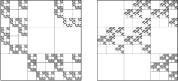
Figure 4. {1,3,5}-{1,4,5} problem in higher dimensional spaces

The authors [49] consider the {1,3,5}-{1,4,5} problem in $\mathbb{R}^{d}$ (see Figure 4) and showed that if the two self-similar sets

$$E_{A}=\bigcup_{a\in A}N^{-1}(E_{A}+a),\quad E_{B}=\bigcup_{b\in B}N^{-1}(E_{B}+b)$$

are totally disconnected, where $A,B\subset\{0,\dots,N-1\}^{d}$, then $E_{A}\simeq E_{B}$ if and only if $\operatorname{card}A=\operatorname{card}B$. Recently, Luo and Lau [28] and Deng and He [10] also studied the IFSs with equal ratios in more general setting than [36, 49] and proved some special cases of Theorem 1.5.

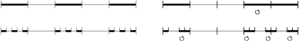
Figure 5. {1,3,5}-{1,4,5} problem with rotation

The authors [51] also proved a rotation version of {1,3,5}-{1,4,5} problem (see Figure 5). Let $S_{1}\colon x\mapsto x/5$, $S_{2}\colon x\mapsto(-x+4)/5$ and $S_{3}\colon x\mapsto(x+4)/5$. The self-similar set $E_{1,-4,5}=\bigcup_{i=1}^{3}S_{i}(E_{1,-4,5})$ is called the $\{1,-4,5\}$-set. Then $E_{1,-4,5}\simeq E_{1,4,5}\simeq E_{1,3,5}$. (In Figure 5, the symbol $\bm{\circlearrowleft}$ means that there is a minus sign in the contraction coefficient of the corresponding similarity. In geometry, this means a rotation by the angle $\pi$.)

As we see, the method of using graph-directed system can deal with various versions of the $\{1,3,5\}$-$\{1,4,5\}$ problem. But this method cannot give a general result for the Lipschitz equivalence problem of self-similar sets since it is in general very hard or even impossible to find a suitable graph-directed system for a given family of self-similar sets. In other word, only very special self-similar sets can be studied by using of graph-directed system.

In this paper, we introduce the blocks to study the self-similar sets and replace the graph-directed system by the interior blocks (see Section 5.1). This new and powerful method leads to deeper insights into geometrical structure of self-similar sets than the method of the graph-directed system. Consequently, we are able to generalize almost all of known results in the OSC and the TDC case. In fact, all the results in [10, 28, 36, 49, 51] are very special cases of Theorem 1.5, which is only a very special corollary of Theorem 1.3. While Theorem 1.6 and 1.7 also generalize the results in [38, 48] under the commensurable case. More important, we think this new method is also useful for the further study on Lipschitz equivalence and other related problems.

3. The Algebraic Properties of Measure Root

This section concerns the algebraic properties of measure root. As a result, we give the proof of Proposition 1.1.

The following lemma is the collection of some algebraic properties of measure root. These properties may be known, we include the proof only for the self-containedness since we don’t find appropriate references (note that $\mathbb{Z}[p]$ is in general not a Dedekind domain).

Lemma 3.1.

Let $p\in(0,1)$. Suppose that there exist positive integers $\lambda_{1},\lambda_{2},\dots,\lambda_{N}$ with $\gcd(\lambda_{1},\dots,\lambda_{N})=1$ such that

$$p^{\lambda_{1}}+p^{\lambda_{2}}+\dots+p^{\lambda_{N}}=1.$$

Then we have the following conclusions.

1. $p^{-1}$ is an algebraic integer and $p^{-1}\in\mathbb{Z}[p]$.

2. The quotient ring $\mathbb{Z}[p]/I$ is finite for every nonzero ideal $I$.

3. For each nonzero ideal $I$ of $\mathbb{Z}[p]$, there exists a positive integer $\ell$ such that $1-p^{\ell}\in I$.

4. $\mathbb{Z}[p]$ is noetherian, i.e., every ideal is finitely generated.

5. For each positive number $a\in\mathbb{Z}[p]$, there exists a polynomial $P$ with positive integer coefficients such that $a=P(p)$. In other words,

   $$\{a>0\colon a\in\mathbb{Z}[p]\}=\mathbb{Z}^{+}[p],$$

   where $\mathbb{Z}^{+}[p]$ is defined by (2.1).

6. Let $a_{1},\dots,a_{m}$ be positive numbers and $I=(a_{1},\dots,a_{m})$ the ideal of $\mathbb{Z}[p]$ generated by $a_{1},\dots,a_{m}$. Then, for each positive number $a\in I$, there exist positive numbers $b_{1},\dots,b_{m}\in\mathbb{Z}[p]$ such that

   $$a=a_{1}b_{1}+a_{2}b_{2}+\dots+a_{m}b_{m}.$$

7. $h(\mathbb{Z}[p])\leq h(\mathbb{Z}[p^{-1}])$.

8. $h(\mathcal{O}_{p})\leq h(\mathbb{Z}[p^{-1}])$, where $\mathcal{O}_{p}$ denotes the ring of all algebraic integers in the field $\mathbb{Q}(p)$.

We remark that the inequalities in Lemma 3.1(g) and (h) may be strict, see Example 3.1 and 3.2. We need the following fact.

Fact 3.1.

The class number $h(\mathbb{Z}[\sqrt{n}\,])>1$ if the nonzero integer $n$ is not square free (i.e., $m^{2}\mid n$ for some integer $m>1$). For this, one can check that the ideal $(m,\sqrt{n})$ is not a principle ideal, where $m$ is a prime number such that $m^{2}\mid n$.

Example 3.1.

Let $p=(\sqrt{10}-3)/2$ be the solution of $4p^{2}+12p=1$. Then

$$h(\mathbb{Z}[p])=h(\mathbb{Z}[\sqrt{10},\tfrac{1}{2}])=1<h(\mathbb{Z}[p^{-1}])=h(\mathbb{Z}[2\sqrt{10}]).$$

To see that $h(\mathbb{Z}[\sqrt{10},\tfrac{1}{2}])=1$, observe that the mapping

$$\pi\colon I\to I^{*}=\{2^{-\ell}\alpha\colon\alpha\in I,\ell\geq 0\}$$

from the nonzero ideal $I$ of $\mathbb{Z}[\sqrt{10}]$ to the nonzero ideal $I^{*}$ of $\mathbb{Z}[\sqrt{10},\tfrac{1}{2}]$ is a surjection, and that $I=aJ$ implies $I^{*}=aJ^{*}$. Then since a nonzero ideal $I$ of $\mathbb{Z}[\sqrt{10}]$ is either a principle ideal or belongs to the same ideal class of $(2,\sqrt{10})$, it follows from $\pi(2,\sqrt{10})=\mathbb{Z}[\sqrt{10},\tfrac{1}{2}]$ that $h(\mathbb{Z}[\sqrt{10},\tfrac{1}{2}])=1$.

Example 3.2.

Let $p=5\sqrt{2}-7$ be the solution of $p^{2}+14p=1$. Then

$$h(\mathcal{O}_{p})=h(\mathbb{Z}[\sqrt{2}])=1<h(\mathbb{Z}[p^{-1}])=h(\mathbb{Z}[5\sqrt{2}]).$$

We remark that in Example 3.1, $h(\mathbb{Z}[p])=1<h(\mathcal{O}_{p})=h(\mathbb{Z}[\sqrt{10}])=2$, while in Example 3.2, $h(\mathcal{O}_{p})=1<h(\mathbb{Z}[p])=h(\mathbb{Z}[5\sqrt{2}])$.

The remainder of this section is devoted to the proof of Lemma 3.1 and Proposition 1.1. We begin with a technical lemma.

Lemma 3.2.

Let

$$\bm{\Xi}=\begin{pmatrix}\xi_{1}&1&0&\ldots\ldots\ldots\ldots&0\\ \xi_{2}&0&1&0&\ldots\ldots\ldots&0\\ \xi_{3}&0&0&1&0&\ldots\ldots&0\\ \vdots&\vdots&\vdots&\vdots&\vdots&\vdots&\vdots&\vdots\\ \vdots&\vdots&\vdots&\vdots&\vdots&\vdots&\vdots&\vdots\\ \xi_{n-2}&0&\ldots\ldots\ldots&0&1&0\\ \xi_{n-1}&0&\ldots\ldots\ldots\ldots&0&1\\ \xi_{n}&0&\ldots\ldots\ldots\ldots\ldots&0\\ \end{pmatrix}$$

be an $n\times n$ matrix, where $\xi_{1},\xi_{2},\dots,\xi_{n}$ are nonnegative integers. Let $\lambda_{1},\dots,\lambda_{m}$ be all the indexes such that $\xi_{\lambda_{i}}>0$. If $\gcd(\lambda_{1},\dots,\lambda_{m})=1$ and $n\in\{\lambda_{1},\dots,\lambda_{m}\}$, i.e., $\xi_{n}>0$, then the matrix $\bm{\Xi}$ is primitive. Moreover, let $p$ be the unique positive solution of the equation $\xi_{1}p+\xi_{2}p^{2}+\dots+\xi_{n}p^{n}=1$ and $\bm{p}=(1,p,\dots,p^{n})$, then

$$\bm{p}\bm{\Xi}=p^{-1}\bm{p}.$$

In other word, the value $p^{-1}$ is the Perron-Frobenius eigenvalue of $\bm{\Xi}$ and the vector $\bm{p}$ is the corresponding left-hand Perron-Frobenius eigenvector.

In what follows, $\bm{A}\geq\bm{B}$ means that each $a_{ij}\geq b_{ij}$ and $\bm{A}>\bm{B}$ that each $a_{ij}>b_{ij}$ for arbitrary matrices $\bm{A}=(a_{ij})$ and $\bm{B}=(b_{ij})$.

Proof.

The equality $\bm{p}\bm{\Xi}=p^{-1}\bm{p}$ is obvious. It remains to show that the matrix $\bm{\Xi}$ is primitive. Let $\bm{A}_{ij}$ be the $n\times n$ matrix such that the $(i,j)$-entry of $\bm{A}_{ij}$ is $1$ and all other entries are zero. Let $\bm{B}=(b_{ij})$ be the $n\times n$ matrix as

$$b_{ij}=\begin{cases}1,&i+1\equiv j\pmod{n};\\ 0,&\text{otherwise}.\end{cases}$$

It follows from the meanings of $\lambda_{1},\dots,\lambda_{m}$ that

$$\bm{\Xi}\geq\bm{B}+\sum_{\lambda_{i}\neq n}\bm{A}_{\lambda_{i}1}.$$

Since $\gcd\{\lambda_{1},\lambda_{2},\dots,\lambda_{m}\}=1$ and $n\in\{\lambda_{1},\lambda_{2},\dots,\lambda_{m}\}$, there exist positive integers $l_{i}$ and $l$ such that

$$\sum_{\lambda_{i}\neq n}l_{i}\cdot\lambda_{i}=ln+1.$$

Observe that $\bm{B}^{k-1}\bm{A}_{k1}=\bm{A}_{11}$ and $\bm{B}^{n}$ is the identity matrix. We have

$$\biggl{(}\bm{B}+\sum_{\lambda_{i}\neq n}\bm{A}_{\lambda_{i}1}\biggr{)}^{ln+1}\geq\bm{B}^{ln+1}+\prod_{\lambda_{i}\neq n}(\bm{B}^{\lambda_{i}-1}\bm{A}_{\lambda_{i}1})^{l_{i}}=\bm{B}+\bm{A}_{11}.$$

Finally, a straightforward computation reveals that $(\bm{B}+\bm{A}_{11})^{2n-3}>\bm{0}$. ∎

The following lemma is a well-known property of the primitive matrix.

Lemma 3.3.

Let $\bm{\Xi}$, $p$ and $\bm{p}$ be as in Lemma 3.2. Suppose that $\bm{q}$ is the right-hand Perron-Frobenius eigenvector of $\bm{\Xi}$ such that $\bm{p}\cdot\bm{q}=1$. Then

$$\lim_{k\to\infty}p^{k}\bm{\Xi}^{k}=\bm{q}\cdot\bm{p}.$$

Now we are able to prove Lemma 3.1 and Proposition 1.1.

Proof of Lemma 3.1.

(a) It is obvious.

(b) First observe that $\mathbb{Z}[p]/(m)$ is finite for every nonzero integer $m$. It remains to show that each nonzero ideal $I$ contains a nonzero integer. Pick a nonzero number $a\in I$. By (a), for $\ell$ large enough, $p^{-\ell}a\in I$ is a algebraic integer. Thus for a fixed such $\ell$, we can find a polynomial $P$ with integer coefficients such that $P(p^{-\ell}a)\in I$ is a nonzero integer.

(c) By (b), we can find two integers $\ell_{2}>\ell_{1}>0$ with $p^{\ell_{1}}-p^{\ell_{2}}\in I$. We have $1-p^{\ell_{2}-\ell_{1}}\in I$ since $p^{-1}\in\mathbb{Z}[p]$ by (a).

(d) Suppose on the contrary that $I$ is an ideal that is not finitely generated. Then the quotient group $I/(a)$ is infinite for all $a\in I$, which contradicts (b) since $I/(a)\subset\mathbb{Z}[p]/(a)$.

(e) Suppose that

$$p^{\lambda_{1}}+p^{\lambda_{2}}+\dots+p^{\lambda_{N}}=\xi_{1}p+\xi_{2}p^{2}+\dots+\xi_{n}p^{n},$$

where $\xi_{n}>0$. Let $\bm{\Xi}$ be the matrix as in Lemma 3.2. Since $\gcd(\lambda_{1},\dots,\lambda_{N})=1$, the conditions of Lemma 3.2 are fulfilled. Let $\bm{p}$ and $\bm{q}$ be the Perron-Frobenius eigenvectors as in Lemma 3.3. Since $a\in\mathbb{Z}[p]$ is positive, there exist $\ell\geq 0$ and a column vector $\bm{a}=(a_{1},a_{2},\dots,a_{n})^{T}$ with integer entries such that $a=p^{\ell}\bm{p}\cdot\bm{a}>0$. Recall that $p^{-1}$ and $\bm{p}$ are the eigenvalue and the eigenvector of the matrix $\bm{\Xi}$, respectively. And so $a=p^{\ell+k}\bm{p}\bm{\Xi}^{k}\bm{a}$ for all $k\geq 0$. By Lemma 3.3,

$$p^{k}\bm{\Xi}^{k}\bm{a}\to\bm{q}\cdot(\bm{p}\cdot\bm{a})>\bm{0}\quad\text{as $k\to\infty$}.$$

This implies that $\bm{\Xi}^{k}\bm{a}>\bm{0}$ for sufficiently large $k$. Thus, Conclusion (e) follows.

(f) We prove this by induction on $m$. The case $m=1$ is obvious. Now suppose this is true for $m-1$, let $a\in(a_{1},\dots,a_{m})$ be a positive number. We have $a=a_{1}b^{\prime}_{1}+\dots+a_{m}b^{\prime}_{m}$ for some $b^{\prime}_{1},\dots,b^{\prime}_{m}\in\mathbb{Z}[p]$. Suppose without loss of generality that $b^{\prime}_{m}>0$. By (c), we can find a positive integer $\ell$ such that $1-p^{\ell}\in(a_{1},\dots,a_{m-1})$. Pick $k$ large enough such that $a-a_{m}b^{\prime}_{m}p^{k\ell}>0$. The proof is completed by the induction assumption since

$$0<a-a_{m}b^{\prime}_{m}p^{k\ell}=a-a_{m}b^{\prime}_{m}+a_{m}b^{\prime}_{m}(1-p^{k\ell})\in(a_{1},\dots,a_{m-1}).$$

(g) For each nonzero ideal $I$ of $\mathbb{Z}[p]$, write $I^{*}=I\cap\mathbb{Z}[p^{-1}]$, then $I^{*}$ is a nonzero ideal of $\mathbb{Z}[p^{-1}]$. It suffices to show the fact that if $I^{*}=aJ^{*}$ for some $a\in\mathbb{R}$, then $I=aJ$, where $I$ and $J$ are two nonzero ideals of $\mathbb{Z}[p]$. Indeed, for each $b\in J$, there exists an integer $\ell$ with $bp^{-\ell}\in J^{*}$, so $abp^{-\ell}\in aJ^{*}=I^{*}$. Thus $ab\in I$, i.e., $aJ\subset I$. By symmetric, $a^{-1}I\subset J$ and so $I=aJ$.

(h) Recall that $p^{-1}$ is an algebraic integer and that $\mathbb{Q}(p)=\mathbb{Q}(p^{-1})$. Together with the fact that $\mathcal{O}_{p}$ is a finitely generated $\mathbb{Z}$-module, we know that there exists a positive integer $m$ such that $m\mathcal{O}_{p}\subset\mathbb{Z}[p^{-1}]$. For each nonzero ideal $I$ of $\mathcal{O}_{p}$, write $I^{*}=mI$, then $I^{*}$ is a nonzero ideal of $\mathbb{Z}[p^{-1}]$. It is obviously that $aI^{*}=J^{*}$ if and only if $aI=J$, where $I$ and $J$ are two nonzero ideals of $\mathcal{O}_{p}$. Therefore, $h(\mathcal{O}_{p})\leq h(\mathbb{Z}[p^{-1}])$. ∎

Proof of Proposition 1.1.

Suppose first that there is an IFS $\mathcal{S}\in\mathrm{TDC}\cap\mathrm{OSC^{E}_{1}}(p,r)$. By the meanings of $p,r$, we can assume that the ratios of $\mathcal{S}$ are $r^{\lambda_{1}},r^{\lambda_{2}},\dots,r^{\lambda_{N}}$, where $\gcd(\lambda_{1},\dots,\lambda_{N})=1$. Then we have

$$p^{\lambda_{1}}+p^{\lambda_{2}}+\dots+p^{\lambda_{N}}=1.$$

The conclusion that $p,r\in(0,1)$ is obvious.

Conversely, fix an integer $\ell>0$ such that $r^{\ell}<1/2$ and $1-p^{\ell}-p^{\ell+1}>0$. By Lemma 3.1(e), there exist nonnegative integers $\ell_{1},\dots,\ell_{m}$ such that

$$p^{-\ell}(1-p^{\ell}-p^{\ell+1})=p^{\ell_{1}}+p^{\ell_{2}}+\dots+p^{\ell_{m}}.$$

Let $\mathcal{S}$ be an IFS satisfying the OSC and consisting of $m+2$ similarities with ratios $r^{\ell}$, $r^{\ell+1}$, $r^{\ell+\ell_{1}},r^{\ell+\ell_{2}},\dots,r^{\ell+\ell_{m}}$. Since all the ratios are less than $1/2$, such IFS does exist on $\mathbb{R}^{d}$ with $2^{d}\geq m+2$. For example, let $\mathcal{S}=\{S_{1},\dots,S_{m+2}\}$ with

$$S_{1} \colon x\mapsto r^{\ell}x+(\underbrace{0,\dots,0,0}_{d})/2, S_{2} \colon x\mapsto r^{\ell+1}x+(\underbrace{0,\dots,0,1}_{d})/2,$$

$$S_{3} \colon x\mapsto r^{\ell+\ell_{1}}x+(\underbrace{0,\dots,1,0}_{d})/2, S_{4} \colon x\mapsto r^{\ell+\ell_{2}}x+(\underbrace{0,\dots,1,1}_{d})/2,$$

$$\dots\dots \dots\dots$$

Then $\mathcal{S}$ satisfies the OSC with the open set $(0,1)^{d}$. Also note that $\gcd(\ell,\ell+1)=1$, so we have $r_{\mathcal{S}}=r$ and $p_{\mathcal{S}}=p$. Therefore, $\mathcal{S}\in\mathrm{TDC}\cap\mathrm{OSC^{E}_{1}}(p,r)\neq\emptyset$. ∎

4. The Ideal of IFS

This section is devoted to the proofs of Theorem 1.3 and Theorem 1.7, which are closely related to the problem of determining the ideal of IFS in $\mathrm{TDC}\cap\mathrm{OSC^{E}_{1}}$. The difficult is that there is no general method to determine such ideals. For our purpose, we consider the problem in two special cases: the self-similar set has the graph-directed structure and the self-similar set generated by IFSs in $\mathscr{S}$, where $\mathscr{S}$ is defined by (1.1).

4.1. The graph-directed structure

The key point of the proof of Theorem 1.3 is the following theorem.

Theorem 4.1.

Suppose that $\mathrm{TDC}\cap\mathrm{OSC^{E}_{1}}(p,r)\neq\emptyset$. Then for each nonzero ideal $I$ of the ring $\mathbb{Z}[p]$, there exists an IFS $\mathcal{S}\in\mathrm{TDC}\cap\mathrm{OSC^{E}_{1}}(p,r)$ such that $I_{\mathcal{S}}=I$.

We make use of the graph-directed sets to prove Theorem 4.1. For convenience, we recall the definition of graph-directed sets (see [30]).

Definition 4.1 (graph-directed sets).

Let $G=(\mathcal{V},\mathcal{E})$ be a directed graph with vertex set $\mathcal{V}$ and directed-edge set $\mathcal{E}$. Suppose that for each edge $e\in\mathcal{E}$, there is a corresponding similarity $S_{e}\colon\mathbb{R}^{d}\to\mathbb{R}^{d}$ of ratio $r_{e}\in(0,1)$.

The graph-directed sets on $G$ with the similarities $\{S_{e}\}_{e\in\mathcal{E}}$ are defined to be the unique nonempty compact sets $\{E_{i}\}_{i\in\mathcal{V}}$ satisfying

(4.1) $$E_{i}=\bigcup_{j\in\mathcal{V}}\bigcup_{e\in\mathcal{E}_{i,j}}S_{e}(E_{j})\qquad\text{for $i\in\mathcal{V}$},$$

where $\mathcal{E}_{i,j}$ is the set of edges staring at $i$ and ending at $j$. In particular, if (4.1) is a disjoint union for each $i\in\mathcal{V}$, we call $\{E_{i}\}_{i\in\mathcal{V}}$ are dust-like graph-directed sets on $(\mathcal{V},\mathcal{E})$.

If the self-similar set $E$ has the graph-directed structure, we can determine its ideal easily. Let $\mathcal{S}\in\mathrm{TDC}\cap\mathrm{OSC^{E}_{1}}(p,r)$. Suppose that $E_{\mathcal{S}}$ is one of the dust-like graph-directed sets $\{E_{i}\}_{i\in\mathcal{V}}$ on $G=(\mathcal{V},\mathcal{E})$, and that for all $e\in\mathcal{E}$, $\log r_{e}/\log r\in\mathbb{N}$. Without loss of generality, we also suppose that $\mathcal{V}=\{0,1,\dots,n\}$ and $E_{\mathcal{S}}=E_{0}$. Let $\mathcal{E}_{i,j}^{k}$ denote the set of sequences of $k$ edges $(e_{1},e_{2},\dots,e_{k})$ which form a directed path from vertex $i$ to vertex $j$. Let $O$ be an open set of $\mathcal{S}$ satisfying the SOSC. We use $\mathcal{V}_{O}$ to denote the set of vertexes $i$ such that there exists $(e_{1},e_{2},\dots,e_{k})\in\mathcal{E}_{0,i}^{k}$ for some $k\geq 1$ satisfying

$$S_{e_{1}}\circ S_{e_{2}}\circ\dots\circ S_{e_{k}}(E_{i})\subset O.$$

Theorem 4.2.

The ideal $I_{\mathcal{S}}$ is generated by $\{\mathcal{H}^{s}(E_{i})/\mathcal{H}^{s}(E_{\mathcal{S}})\colon i\in\mathcal{V}_{O}\}$, where $s=\operatorname{\dim_{H}}E_{\mathcal{S}}$.

The proof of Theorem 4.2 will be given in Section 5.3 since it requires a basic fact about the ideal of IFS (Remark 5.6). We give an example here.

Example 4.1.

Let $\mathcal{S}$ be as in Example 1.3. Let $E_{0}=E_{\mathcal{S}}$, $E_{1}=-rE_{\mathcal{S}}\cup E_{\mathcal{S}}$ and $E_{2}=-E_{\mathcal{S}}+E_{\mathcal{S}}$. It is easy to check that $E_{0}$, $E_{1}$ and $E_{2}$ forms a family of graph-directed sets. Let $O=(0,1)$, then $\mathcal{V}_{O}=\{1,2\}$. By Theorem 4.2,

$$I_{\mathcal{S}}=(\mathcal{H}^{s}(E_{1})/\mathcal{H}^{s}(E_{0}),\mathcal{H}^{s}(E_{2})/\mathcal{H}^{s}(E_{0}))=(p+1,2).$$

By Theorem 4.2, we are able to give the proof of Theorem 4.1.

Proof of Theorem 4.1.

Fix a nonzero ideal $I$ of $\mathbb{Z}[p]$. By Lemma 3.1(c), there exists a positive integer $\ell$ such that $1-p^{\ell}\in I$. We can further require that $r^{\ell}<1/6$ since $1-p^{k\ell}\in I$ for all $k\geq 1$. By Lemma 3.1(d), we can choose positive numbers $a_{1},a_{2},\dots,a_{m}\in\mathbb{Z}[p]$ such that $I=(a_{1},\dots,a_{m})$. By Lemma 3.1(f), there exist positive numbers $b_{1},\dots,b_{m}\in I$ such that

(4.2) $$1-p^{\ell}=a_{1}b_{1}+\dots+a_{m}b_{m}.$$

By Lemma 3.1(e), for $1\leq i\leq m$, there exist nonnegative integers $u_{i,j}$ ($1\leq j\leq N_{i}$) and positive integers $v_{i,j}$ with $r^{v_{i,j}}<1/6$ ($1\leq j\leq M_{i}$) such that

(4.3) $$a_{i} =p^{u_{i,1}}+p^{u_{i,2}}+\dots+p^{u_{i,N_{i}}},$$

$$b_{i} =p^{v_{i,1}}+p^{v_{i,2}}+\dots+p^{v_{i,M_{i}}}.$$

We can further require that

(4.4) $$u_{1,1}+1=u_{1,2}$$

since there exists a nonnegative integer $u$ such that $a_{1}-p^{u}-p^{u+1}>0$, then set $u_{1,1}=u$, $u_{2,1}=u+1$ and apply Lemma 3.1(e) to $a_{1}-p^{u}-p^{u+1}$. Finally, choose a positive integer $d$ such that

(4.5) $$2^{d}\geq\max(N_{1},N_{2},\dots,N_{m})\quad\text{and}\quad 2^{d}\geq M_{1}+M_{2}+\dots+M_{m}.$$

Now we are ready to construct the desired IFS $\mathcal{S}$. In the remainder of this proof, we use $\bm{x}$ and $\bm{y}$ to denote the points in $\mathbb{R}^{d}$. For $\Lambda\subset\{1,2,\dots,d\}$, define an isometric mapping $T_{\Lambda}\colon\mathbb{R}^{d}\to\mathbb{R}^{d}$ by

(4.6) $$(T_{\Lambda}\bm{x})_{i}=\begin{cases}x_{i},&i\notin\Lambda,\\ -x_{i},&i\in\Lambda,\end{cases}\quad\text{for $\bm{x}=(x_{1},\dots,x_{d})\in\mathbb{R}^{d}$}.$$

Since $2^{d}\geq\max(N_{1},\dots,N_{m})$, for each $i\in\{1,2,\dots,m\}$, we can choose distinct

$$\Lambda_{i,1},\Lambda_{i,2}\dots,\Lambda_{i,N_{i}}\subset\{1,\dots,d\},$$

and then define an IFS $\mathcal{T}_{i}$ as

(4.7) $$\mathcal{T}_{i}=\bigl{\{}r^{u_{i,1}}T_{\Lambda_{i,1}},r^{u_{i,2}}T_{\Lambda_{i,2}},\dots,r^{u_{i,N_{i}}}T_{\Lambda_{i,N_{i}}}\bigr{\}}.$$

Let

$$Y=\bigl{\{}\bm{y}=(y_{1},\dots,y_{d})\in\mathbb{R}^{d}\colon\text{$y_{i}=1/3$ or $2/3$ for $i=1,\dots,d$}\}.$$

Since $2^{d}\geq M_{1}+\dots+M_{m}$, we can choose distinct points $\bm{y}_{i,j}\in Y$ for $1\leq i\leq m$ and $1\leq j\leq M_{i}$. Define a contracting similarity $S_{0}\colon\bm{x}\mapsto r^{\ell}\bm{x}$ on $\mathbb{R}^{d}$ and IFSs

(4.8) $$\mathcal{S}_{i,j}=\bigl{\{}r^{v_{i,j}}T+\bm{y}_{i,j}\colon T\in\mathcal{T}_{i}\bigr{\}}$$

for $1\leq i\leq m$, $1\leq j\leq M_{i}$. Finally, define

$$\mathcal{S}=\{S_{0}\}\cup\bigcup_{i=1}^{m}\bigcup_{j=1}^{M_{i}}\mathcal{S}_{i,j}.$$

It remains to show that $\mathcal{S}\in\mathrm{TDC}\cap\mathrm{OSC^{E}_{1}}(p,r)$ and $I_{\mathcal{S}}=I$.

We first prove that $\mathcal{S}\in\mathrm{OSC^{E}_{1}}(p,r)$. Note that the ratios of $\mathcal{S}$ are

$$r^{\ell}\quad\text{and}\quad r^{u_{i,j}+v_{i,j^{\prime}}}\ (1\leq i\leq m,1\leq j\leq N_{i},1\leq j^{\prime}\leq M_{i}).$$

By (4.4), we have $r_{\mathcal{S}}=r$. By (4.2) and (4.3), we have $p_{\mathcal{S}}=p$. We will show that $\mathcal{S}$ satisfies the OSC for the open set $(0,1)^{d}$. Note that the ratios of $\mathcal{S}$ are all less than $1/6$ since $r^{\ell}<1/6$, $r^{v_{i,j}}<1/6$ and $u_{i,j}\geq 0$. And so $S_{0}(0,1)^{d}\subset(0,1/6)^{d}$; $S(0,1)^{d}\subset(-1/6,1/6)^{d}+\bm{y}_{i,j}$ for $S\in\mathcal{S}_{i,j}$. Therefore, $S(0,1)^{d}\subset(0,1)^{d}$ for all $S\in\mathcal{S}$. On the other hand, for distinct $S,S^{\prime}\in\mathcal{S}$, we need to show $S(0,1)^{d}\cap S^{\prime}(0,1)^{d}=\emptyset$. There are three cases to consider.

Case 1:

One of $S,S^{\prime}$ is $S_{0}$. Then there exists some $\bm{y}\in Y$ such that

$$S(0,1)^{d}\cap S^{\prime}(0,1)^{d}\subset(0,1/6)^{d}\cap\bigl{(}(-1/6,1/6)^{d}+\bm{y}\bigr{)}=\emptyset.$$

Case 2:

$S\in\mathcal{S}_{i,j}$ and $S^{\prime}\in\mathcal{S}_{i^{\prime},j^{\prime}}$ with $(i,j)\neq(i^{\prime},j^{\prime})$. Then the corresponding $\bm{y}_{i,j},\bm{y}_{i^{\prime},j^{\prime}}\in Y$ are distinct. And so

$$S(0,1)^{d}\cap S^{\prime}(0,1)^{d}\subset\bigl{(}(-1/6,1/6)^{d}+\bm{y}_{i,j}\bigr{)}\cap\bigl{(}(-1/6,1/6)^{d}+\bm{y}_{i^{\prime},j^{\prime}}\bigr{)}=\emptyset.$$

Case 3:

$S,S^{\prime}\in\mathcal{S}_{i,j}$. By the definition of $\mathcal{S}_{i,j}$, we have $S(0,1)^{d}\cap S^{\prime}(0,1)^{d}=\emptyset$.

This completes the proof of $\mathcal{S}\in\mathrm{OSC^{E}_{1}}(p,r)$.

Let $E_{0}=E_{\mathcal{S}}$ be the self-similar set generated by $\mathcal{S}$ and $E_{i}=\bigcup_{T\in\mathcal{T}_{i}}T(E_{0})$ for $1\leq i\leq m$. Define $S_{i,j}\colon x\mapsto r^{v_{i,j}}x+\bm{y}_{i,j}$ for $1\leq i\leq m$, $1\leq j\leq M_{i}$. The proof of $\mathcal{S}\in\mathrm{TDC}$ and $I_{\mathcal{S}}=I$ is based on the fact that the sets $\{E_{i}\}_{i=0}^{m}$ are dust like graph-directed sets. Indeed, we have

(4.9) $$E_{0}=S_{0}(E_{0})\cup\bigcup_{i=1}^{m}\bigcup_{j=1}^{M_{i}}S_{i,j}(E_{i}),$$

and for $1\leq i\leq m$,

$$E_{i}=\bigcup_{T\in\mathcal{T}_{i}}T(E_{0})=\bigcup_{T\in\mathcal{T}_{i}}T\circ S_{0}(E_{0})\cup\bigcup_{T\in\mathcal{T}_{i}}\bigcup_{i^{\prime}=1}^{m}\bigcup_{j=1}^{M_{i^{\prime}}}T\circ S_{i^{\prime},j}(E_{i^{\prime}})\\ =\bigcup_{T\in\mathcal{T}_{i}}S_{0}\circ T(E_{0})\cup\bigcup_{T\in\mathcal{T}_{i}}\bigcup_{i^{\prime}=1}^{m}\bigcup_{j=1}^{M_{i^{\prime}}}T\circ S_{i^{\prime},j}(E_{i^{\prime}})$$

since $T\circ S_{0}=S_{0}\circ T$ for $T\in T_{i}$. It follows from $E_{i}=\bigcup_{T\in\mathcal{T}_{i}}T(E_{0})$ that

(4.10) $$E_{i}=S_{0}(E_{i})\cup\bigcup_{T\in\mathcal{T}_{i}}\bigcup_{i^{\prime}=1}^{m}\bigcup_{j=1}^{M_{i^{\prime}}}T\circ S_{i^{\prime},j}(E_{i^{\prime}})\quad\text{for $1\leq i\leq m$}.$$

We will show that all the unions in (4.9) and (4.10) are disjoint. By the definition of $\mathcal{S}$, we know that $E_{0}\subset[0,1]^{d}$, $E_{0}\setminus(0,1)^{d}=\{\bm{0}\}$ and $E_{i}\subset(-1,1)^{d}$ for all $1\leq i\leq m$. Note that the ratios of $S_{0}$ and $S_{i,j}$ are $r^{\ell}$ and $r^{v_{i,j}}$, all less than $1/6$. This means

$$S_{0}(E_{0})\subset[0,1/6]^{d},\quad S_{i,j}(E_{i})\subset(-1/6,1/6)^{d}+\bm{y}_{i,j}.$$

Recall that $\bm{y}_{i,j}\in Y$, we have

$$\bigcup_{i=1}^{m}\bigcup_{j=1}^{M_{i}}S_{i,j}(E_{i})\subset(1/6,5/6)^{d},$$

and

(4.11) $$S_{i,j}(E_{i})\cap S_{i^{\prime},j^{\prime}}(E_{i^{\prime}})=\emptyset\quad\text{when $(i,j)\neq(i^{\prime},j^{\prime})$},$$

since $\bm{y}_{i,j}\neq\bm{y}_{i^{\prime},j^{\prime}}$. Therefore, the unions in (4.9) are disjoint. For the unions in (4.10), observe that, for $1\leq i\leq m$ and distinct $T,T^{\prime}\in\mathcal{T}_{i}$, $T(0,1)^{d}\cap T^{\prime}[0,1]^{d}=\emptyset$ by the definition of $\mathcal{T}_{i}$. There are two results follow from the observation. The first is

$$\bigcup_{i^{\prime}=1}^{m}\bigcup_{j=1}^{M_{i^{\prime}}}T\circ S_{i^{\prime},j}(E_{i^{\prime}})\cap\bigcup_{i^{\prime}=1}^{m}\bigcup_{j=1}^{M_{i^{\prime}}}T^{\prime}\circ S_{i^{\prime},j}(E_{i^{\prime}})\subset T(1/6,5/6)^{d}\cap T^{\prime}(1/6,5/6)^{d}=\emptyset$$

for distinct $T,T^{\prime}\in\mathcal{T}_{i}$. The second is, for $T\in\mathcal{T}_{i}$, $1\leq i^{\prime}\leq m$ and $1\leq j\leq M_{i^{\prime}}$,

$$T\circ S_{i^{\prime},j}(E_{i^{\prime}})\cap S_{0}(E_{i})=T\circ S_{i^{\prime},j}(E_{i^{\prime}})\cap\bigcup_{T^{\prime}\in\mathcal{T}_{i}}T^{\prime}\circ S_{0}(E_{0})\\ =T\circ S_{i^{\prime},j}(E_{i^{\prime}})\cap T\circ S_{0}(E_{0})=\emptyset$$

since $S_{i^{\prime},j}(E_{i^{\prime}})\cap S_{0}(E_{0})=\emptyset$. It follows from the two results and (4.11) that the unions in (4.10) are also disjoint. Thus, we have proved that the sets $\{E_{i}\}_{i=0}^{m}$ are dust like graph-directed sets, and so $\mathcal{S}\in\mathrm{TDC}$ follows.

Finally, we turn to prove that $I_{\mathcal{S}}=I$ by making use of Theorem 4.2. Let $O=(0,1)^{d}$, then $\mathcal{V}_{O}=\{1,2,\dots,m\}$. For $1\leq i\leq m$, we have

$$\mathcal{H}^{s}(E_{i})=\sum_{T\in\mathcal{T}_{i}}\mathcal{H}^{s}(T(E_{0}))=(p^{u_{i,1}}+p^{u_{i,2}}+\dots+p^{u_{i,N_{i}}})\mathcal{H}^{s}(E_{0})=a_{i}\mathcal{H}^{s}(E_{0})$$

by (4.3) and (4.7). Therefore, we have $I_{\mathcal{S}}=(a_{1},\dots,a_{m})=I$. ∎

Figure 6. The structure of $E_{\mathcal{S}}$ in Example 4.2

Example 4.2.

Let $r=1/10$ and $p=\sqrt{10}-3$ be the positive solution of the equation $p^{2}+6p=1$. Let $I=(2,\sqrt{10})$ be an ideal of the ring $\mathbb{Z}[p]=\mathbb{Z}[\sqrt{10}]$. It is worth noting that $I$ is not a principle ideal.

It follows from Proposition 1.1 that $\mathrm{TDC}\cap\mathrm{OSC^{E}_{1}}(p,r)\neq\emptyset$. We will construct an IFS $\mathcal{S}\in\mathrm{TDC}\cap\mathrm{OSC^{E}_{1}}(p,r)$ such that $I_{\mathcal{S}}=I$ according to the proof of Theorem 4.1.

Observe that $I=(2,p+1)$ and $1-p=p(p+1)+2p\cdot 2$. By (4.2), (4.3), (4.4) and (4.5), we may set

$$\begin{cases}a_{1}=1+p,\\ a_{2}=2=1+1,\end{cases}\quad\begin{cases}b_{1}=p,\\ b_{2}=2p=p+p,\end{cases}\begin{cases}\ell=1,\\ d=2.\end{cases}$$

By (4.6), (4.7) and (4.8), we may set

$$\mathcal{T}_{1}=\{T_{\emptyset},r\cdot T_{\{1,2\}}\},\quad\mathcal{T}_{2}=\{T_{\emptyset},T_{\{1\}}\},$$

$S_{0}=rT_{\emptyset}$ and

$$\mathcal{S}_{1,1}=\bigl{\{}rT_{\emptyset}+(2/3,2/3),r^{2}T_{\{1,2\}}+(2/3,2/3)\bigr{\}},$$

$$\mathcal{S}_{2,1}=\bigl{\{}rT_{\emptyset}+(2/3,1/3),rT_{\{1\}}+(2/3,1/3)\bigr{\}},$$

$$\mathcal{S}_{2,2}=\bigl{\{}rT_{\emptyset}+(1/3,2/3),rT_{\{1\}}+(1/3,2/3)\bigr{\}}.$$

Finally, let $\mathcal{S}=\{S_{0}\}\cup\mathcal{S}_{1,1}\cup\mathcal{S}_{2,1}\cup\mathcal{S}_{2,2}$, see Figure 6 for the corresponding self-similar set $E_{\mathcal{S}}$. By the proof of Theorem 4.1, we know that $I_{\mathcal{S}}=I$.

We also need the following special version of Jordan-Zassenhaus Theorem (see, e.g., [7]) to prove Theorem 1.3.

Jordan-Zassenhaus Theorem.

Suppose that $\alpha$ is an algebraic integer, then the class number $h(\mathbb{Z}[\alpha])$ is finite.

We remark that $\mathbb{Z}[\alpha]$ is in general not a Dedekind domain, so the conclusion on the finiteness of class number $h(\mathbb{Z}[\alpha])$ cannot be derived directly by the corresponding result of Dedekind domain.

Proof of Theorem 1.3.

By Theorem 1.2 and 4.1, we have $h_{\mathrm{L}}(p,r)=h(\mathbb{Z}[p])$ when $\mathrm{TDC}\cap\mathrm{OSC^{E}_{1}}(p,r)\neq\emptyset$. Then by Lemma 3.1(g), we have $h_{\mathrm{L}}(p,r)=h(\mathbb{Z}[p])\leq h(\mathbb{Z}[p^{-1}])$. Finally, since $p^{-1}$ is an algebraic integer (Lemma 3.1(a)), by the Jordan-Zassenhaus Theorem, the class number $h_{\mathrm{L}}(p,r)\leq h(\mathbb{Z}[p^{-1}])$ is finite. ∎

4.2. Principle ideal

Let $\mathcal{S}=\{S_{1},S_{2},\dots,S_{N}\}$ be an IFS satisfying the OSC. We write $\mathscr{O}_{\mathcal{S}}$ to denote all the open sets satisfying the OSC for the IFS $\mathcal{S}$ and $\partial_{\mathcal{S}}=E_{\mathcal{S}}\setminus\bigcup_{O\in\mathscr{O}_{\mathcal{S}}}O$, where $E_{\mathcal{S}}$ is the self-similar set generated by $\mathcal{S}$. Notice that $\partial_{\mathcal{S}}=\emptyset$ if and only if $\mathcal{S}$ satisfies the SSC. We say that a point $x\in\partial_{\mathcal{S}}$ is separated if there is a finite word $\bm{i}=i_{1}\dots i_{n}\in\{1,\dots,N\}^{n}$ such that

(4.12) $$S_{\bm{i}}(x)\notin\partial_{\mathcal{S}}\quad\text{and}\quad S_{\bm{i}}(x)\notin S_{\bm{j}}(E_{\mathcal{S}})$$

for every word $\bm{j}$ of the same length as $\bm{i}$ but $\bm{j}\neq\bm{i}$, where $S_{\bm{i}}=S_{i_{1}}\circ\dots\circ S_{i_{n}}$.

We need the following theorem to prove Theorem 1.7, which is also of interesting in itself.

Theorem 4.3.

Let $\mathcal{S}\in\mathrm{TDC}\cap\mathrm{OSC^{E}_{1}}$. If the points in $\partial_{\mathcal{S}}$ are all separated, then $I_{\mathcal{S}}=\mathbb{Z}[p_{\mathcal{S}}]$.

Proof.

For each $x\in\partial_{\mathcal{S}}$, let $\bm{i}_{x}$ be a word of finite length satisfying (4.12). Choose a compact subset $F_{x}\subset E_{\mathcal{S}}$ containing $x$ such that $E_{\mathcal{S}}\setminus F_{x}$ is also compact and $S_{\bm{i}_{x}}(F_{x})\cap S_{\bm{j}}(E_{\mathcal{S}})=\emptyset$ for every word $\bm{j}$ of same length as $\bm{i}_{x}$ but $\bm{j}\neq\bm{i}_{x}$. Such $F_{x}$ does exist since $E_{\mathcal{S}}$ is totally disconnected and $\bm{i}_{x}$ satisfies (4.12). We can further require $S_{\bm{i}_{x}}(F_{x})$ to be an interior separated set due to $S_{\bm{i}_{x}}(x)\notin\partial_{\mathcal{S}}$. Note that $F_{x}$ is also an open subset in the topology space $E_{\mathcal{S}}$. So $\{F_{x}\}_{x}$ is an open cover of the compact set $\partial_{\mathcal{S}}$, thus we have a finite sub-cover $F_{1}$, …, $F_{n}$ and the corresponding words $\bm{i}_{1}$, …, $\bm{i}_{n}$. Let

$$F^{*}_{0}=E_{\mathcal{S}}\setminus\bigcup_{k=1}^{n}F_{k},\quad F^{*}_{1}=F_{1},\quad F^{*}_{2}=F_{2}\setminus F_{1},\ldots,\quad F^{*}_{n}=F_{n}\setminus\bigcup_{k=1}^{n-1}F_{k}.$$

Then $\{F^{*}_{k}\}_{k=0}^{n}$ is a disjoint cover of $E_{\mathcal{S}}$. We claim that $\mu_{\mathcal{S}}(F^{*}_{k})\in I_{\mathcal{S}}$ for all $0\leq k\leq n$. Then

$$\sum_{k=0}^{n}\mu_{\mathcal{S}}(F^{*}_{k})=\mu_{\mathcal{S}}(E_{\mathcal{S}})=1\in I_{\mathcal{S}}.$$

Thus $I_{\mathcal{S}}=\mathbb{Z}[p_{\mathcal{S}}]$. It remains to prove the claim. For $1\leq k\leq n$, observe that $S_{\bm{i}_{k}}(F^{*}_{k})$ are all interior separated sets. And so $\mu_{\mathcal{S}}(F^{*}_{k})\in I_{\mathcal{S}}$ for $1\leq k\leq n$ since $p_{\mathcal{S}}^{-1}\in\mathbb{Z}[p_{\mathcal{S}}]$ (Lemma 3.1(a)). For $F^{*}_{0}$, since $F^{*}_{0}$ is compact and each point in $F^{*}_{0}$ can be covered by an interior separated set, we have $F^{*}_{0}$ is a finite union of interior separated sets. Thus the claim $\mu_{\mathcal{S}}(F^{*}_{0})\in I_{\mathcal{S}}$ follows. ∎

Proof of Theorem 1.7.

According to Theorem 4.3, we only need to prove that the points in $\partial_{\mathcal{S}}$ are all separated. For this, fix a point $x_{0}\in\partial_{\mathcal{S}}$. Let $F$ be an interior separated set. It is easy to see that, for $n$ large enough, there is a $\Lambda\subset\{1,\dots,N\}^{n}$ such that

$$F=\bigcup_{\bm{i}\in\Lambda}S_{\bm{i}}(E_{\mathcal{S}}).$$

Choose a word in $\Lambda$, say $\bm{i}^{*}$. If $S_{\bm{i}^{*}}(x_{0})\notin S_{\bm{j}}(E_{\mathcal{S}})$ for all $\bm{j}\in\Lambda$ and $\bm{j}\neq\bm{i}^{*}$, then $x_{0}$ is separated since $F$ is an interior separated set. Thus, the proof is completed. Otherwise, suppose that $S_{\bm{i}^{*}}(x_{0})\in S_{\bm{j}}(E_{\mathcal{S}})$ for some $\bm{j}$ other than $\bm{i}^{*}$. Let $O$ be the convex open set satisfying the OSC. Since $S_{\bm{i}^{*}}(O)\cap S_{\bm{j}}(O)=\emptyset$, by convexity, there is a liner function $H$ such that $H(x)<H(y)$ for all $x\in S_{\bm{i}^{*}}(O)$ and all $y\in S_{\bm{j}}(O)$. Since $S_{\bm{i}^{*}}(x_{0})\in\overline{S_{\bm{i}^{*}}(O)}\cap\overline{S_{\bm{j}}(O)}$, we have

$$H(S_{\bm{i}^{*}}(x_{0}))=\sup_{x\in S_{\bm{i}^{*}}(O)}H(x)=\max_{x\in S_{\bm{i}^{*}}(E_{\mathcal{S}})}H(x).$$

Since each $S\in\mathcal{S}$ has the form $S\colon x\mapsto r_{S}\bm{A}x+b_{S}$ with $r_{S}\in(0,1)$, we have

$$S_{\bm{i}}\colon x\mapsto r_{\bm{i}}\bm{A}^{n}x+b_{\bm{i}}\quad\text{for all $\bm{i}\in\Lambda$}.$$

It follows that

$$H(S_{\bm{i}}(x_{0}))=\sup_{x\in S_{\bm{i}}(O)}H(x)=\max_{x\in S_{\bm{i}}(E_{\mathcal{S}})}H(x)\quad\text{for all $\bm{i}\in\Lambda$}.$$

And so $H(S_{\bm{j}}(x_{0}))>H(S_{\bm{i}^{*}}(x_{0}))$. Now let $\Lambda_{1}$ denote the set of all $\bm{i}\in\Lambda$ such that $H(S_{\bm{i}}(x_{0}))>H(S_{\bm{i}^{*}}(x_{0}))$. We have

• $\Lambda_{1}\subsetneq\Lambda$ (since $\bm{i}^{*}\notin\Lambda_{1}$).

• For $\bm{i}\in\Lambda_{1}$, if $S_{\bm{i}}(x_{0})\in S_{\bm{j}}(E_{\mathcal{S}})$ for some $\bm{j}\in\Lambda$, then $\bm{j}\in\Lambda_{1}$ (since $H(S_{\bm{i}}(x_{0}))\leq H(S_{\bm{j}}(x_{0}))$).

Repeat the above argument with replacing $\Lambda$ by $\Lambda_{1}$, then either we find a word $\bm{i}^{*}\in\Lambda_{1}$ such that $S_{\bm{i}^{*}}(x_{0})\notin S_{\bm{j}}(E_{\mathcal{S}})$ for all $\bm{j}\in\Lambda_{1}$ but $\bm{j}\neq\bm{i}^{*}$, this means $x_{0}$ is separated, or we get a subset $\Lambda_{2}\subsetneq\Lambda_{1}$ such that for $\bm{i}\in\Lambda_{2}$, if $S_{\bm{i}}(x_{0})\in S_{\bm{j}}(E_{\mathcal{S}})$ for some $\bm{j}\in\Lambda_{1}$, then $\bm{j}\in\Lambda_{2}$. If the latter case happens, then we repeat the argument again. The process stops when we find a desired word $\bm{i}^{*}$ to show that $x_{0}$ is separated. This completes the proof since $\Lambda$ is finite. ∎

5. The Blocks Decomposition of Self-similar Sets

To understand the geometric structure of self-similar sets generated by IFSs $\mathcal{S}\in\mathrm{TDC}\cap\mathrm{OSC^{E}_{1}}$, we shall make use of the blocks decomposition. Indeed, the whole proof of our result is base on it.

In this section, we introduce the basic definitions of blocks decomposition and give some important properties. From now on, fix an $\mathcal{S}=\{S_{1},S_{2},\dots,S_{N}\}\in\mathrm{TDC}\cap\mathrm{OSC^{E}_{1}}$. For notational convenience, we will write $E_{\mathcal{S}}$, $\mu_{\mathcal{S}}$, $r_{\mathcal{S}}$ and $p_{\mathcal{S}}$ as $E$, $\mu$, $r$ and $p$, respectively. Let $r_{i}$ be the contraction ratio of $S_{i}$ for $1\leq i\leq N$ and $s=\operatorname{\dim_{H}}E$. Write

(5.1) $$\lambda_{i}=\log r_{i}/\log r\quad\text{and}\quad\lambda=\max_{1\leq i\leq N}\lambda_{i}-1.$$

Recall that $\gcd(\lambda_{1},\dots,\lambda_{N})=1$. For $\bm{i}=i_{1}i_{2}\dots i_{n}\in\{1,2,\dots,N\}^{n}$, write $\bm{i}^{-}=i_{1}i_{2}\dots i_{n-1}$ and

(5.2) $$S_{\bm{i}}=S_{i_{1}}\circ S_{i_{2}}\circ\dots\circ S_{i_{n}},\quad r_{\bm{i}}=r_{i_{1}}r_{i_{2}}\cdots r_{i_{n}},\quad p_{\bm{i}}=r_{\bm{i}}^{s}.$$

Define

(5.3) $$\mathcal{S}_{k}=\bigl{\{}S_{\bm{i}}\colon r_{\bm{i}}\leq r^{k}<r_{\bm{i}^{-}}\bigr{\}}.$$

5.1. The definition of blocks decomposition

Definition 5.1 (level-$k$ blocks decomposition).

The decomposition $E=\bigcup_{j=1}^{n_{k}}B_{k,j}$ is called the level-$k$ blocks decomposition of $E$ ($k\geq 0$), if each set

$$\bigl{\{}x\colon\operatorname{dist}(x,B_{k,j})<r^{k}|E|/2\bigr{\}}$$

is connected for $1\leq j\leq n_{k}$ and

$$\operatorname{dist}(B_{k,i},B_{k,j})\geq r^{k}|E|,\quad\text{for $i\neq j$},$$

where $|E|$ denotes the diameter of $E$. The set $B_{k,j}$ is called a level-$k$ block of $\mathcal{S}$. The family of all the level-$k$ blocks will be denoted by $\mathscr{B}_{k}$. Write $\mathscr{B}=\bigcup_{k\geq 0}\mathscr{B}_{k}$.

Remark 5.1.

For $B\in\mathscr{B}_{k}$, write $\mathcal{S}_{B}=\{S\in\mathcal{S}_{k}\colon S(E)\subset B\}$. According to above definition, it is easy to check that $B=\bigcup_{S\in\mathcal{S}_{B}}S(E)$.

We shall use the natural measure $\mu$ to describe the size of blocks. Notice that $r_{\bm{i}}\in\{r^{k},r^{k+1},\dots,r^{k+\lambda}\}$ for $S_{\bm{i}}\in\mathcal{S}_{k}$. This leads to the following definition.

Definition 5.2 (measure polynomial).

For $B\in\mathscr{B}_{k}$ and $0\leq\ell\leq\lambda$, write

$$\xi_{B,\ell}=\operatorname{card}\bigl{\{}S\in\mathcal{S}_{B}\colon\text{the ratio of $S$ is $r^{k+\ell}$}\bigr{\}}.$$

The polynomial

$$P_{B}\colon t\mapsto\xi_{B,0}+\xi_{B,1}t+\dots+\xi_{B,\lambda}t^{\lambda}$$

is called the measure polynomial of level-$k$ block $B$. Write

$$\mathcal{P}_{k}=\left\{P_{B}\colon B\in\mathscr{B}_{k}\right\}\quad\text{and}\quad\mathcal{P}=\bigcup_{k=0}^{\infty}\mathcal{P}_{k}.$$

Remark 5.2.

For $B\in\mathscr{B}_{k}$, we have $\mu(B)=p^{k}P_{B}(p)$. This is why we call $P_{B}$ the measure polynomial and $p$ the measure root of $\mathcal{S}$.

Remark 5.3.

The measure polynomial of a block $B$ depends not only on $B$ but also on the level of $B$ since the level of $B$ may be not unique. For example, let $\mathcal{S}=\{S_{1},S_{2}\}$ with $S_{1}\colon x\mapsto x/9$ and $S_{2}\colon x\mapsto x/3+2/3$. Then $r_{\mathcal{S}}=1/3$ and

$$\mathscr{B}_{1}=\bigl{\{}S_{1}(E_{\mathcal{S}}),S_{2}(E_{\mathcal{S}})\bigr{\}},\quad\mathscr{B}_{2}=\bigl{\{}S_{1}(E_{\mathcal{S}}),S_{2}\circ S_{1}(E_{\mathcal{S}}),S_{2}\circ S_{2}(E_{\mathcal{S}})\bigr{\}}.$$

Note that $S_{1}(E_{\mathcal{S}})\subset\mathscr{B}_{1}\cap\mathscr{B}_{2}$, so the level of $S_{1}(E_{\mathcal{S}})$ may be $1$ or $2$. Consequently, the measure polynomial of $S_{1}(E_{\mathcal{S}})$ may be $t\mapsto t$ for level-$1$ or $t\mapsto 1$ for level-$2$.

Now we introduce the definition of interior blocks, which is the key to our study.

Definition 5.3 (interior block).

For $k\geq 0$, $B\in\mathscr{B}_{k}$ is called a level-$k$ interior block if $\operatorname{dist}(B,O^{c})\geq r^{k}|E|$ for some open set $O$ satisfying the SOSC. While $B\in\mathscr{B}_{k}$ is called a level-$k$ boundary block if $B$ is not a level-$k$ interior block. Let $\mathscr{B}^{\circ}_{k}$ and $\mathscr{B}^{\partial}_{k}$ denote the family of all level-$k$ interior blocks and the family of all level-$k$ boundary blocks, respectively. Write

$$\mathscr{B}^{\circ}=\bigcup_{k\geq 0}\mathscr{B}^{\circ}_{k},\quad\mathcal{P}^{\circ}_{k}=\left\{P_{B}\colon B\in\mathscr{B}^{\circ}_{k}\right\},\quad\mathcal{P}^{\circ}=\bigcup_{k=0}^{\infty}\mathcal{P}^{\circ}_{k}.$$

Remark 5.4.

Suppose that $B\in\mathscr{B}^{\circ}_{k}$, then

1. for all level-$l$ blocks $A\subset B$, we have $A\in\mathscr{B}^{\circ}_{l}$;

2. suppose that $r_{\bm{i}}=r^{l}$, then $S_{\bm{i}}(B)\in\mathscr{B}^{\circ}_{k+l}$ and $P_{S_{\bm{i}}(B)}=P_{B}$.

For further study of blocks decomposition, we introduce some more notations.

Definition 5.4 (notations).

(a) Let $\mathscr{C}$ be a family of sets. Write

$$\bigsqcup\mathscr{C}=\bigcup_{C\in\mathscr{C}}C.$$

(b) Let $\mathscr{A}\subset\mathscr{B}_{l}$ be a nonempty family of level-$l$ blocks. For $k\geq 0$, write

$$\mathscr{B}_{k}(\mathscr{A})=\Bigl{\{}B\in\mathscr{B}_{l+k}\colon B\subset\bigsqcup\mathscr{A}\Bigr{\}}.$$

(c) Let $A\in\mathscr{B}_{l}$ be a level-$l$ block. For $k\geq 0$, write

$$\mathscr{B}^{\circ}_{k}(A)=\{B\in\mathscr{B}^{\circ}_{l+k}\colon B\subset A\},\quad\mathscr{B}^{\partial}_{k}(A)=\{B\in\mathscr{B}^{\partial}_{l+k}\colon B\subset A\}$$

and $\mathscr{B}_{k}(A)=\{B\in\mathscr{B}_{l+k}\colon B\subset A\}$.

The interior blocks have many advantages. The first is that, under the OSC, different small copies of the self-similar set may has overlaps, but the intersection of interior blocks in different small copies must be empty. The second is that blocks in an interior block are still interior blocks (see Remark 5.4(a)). This means that we recover a form of disjointness result for interior blocks. Therefore, the geometrical structure of interior blocks is like the self-similar sets satisfying the SSC in some sense. The last but not the least is the following lemma, which reveals the relationship between the measure polynomials of interior blocks and the ideal of $\mathcal{S}$.

Lemma 5.1.

Let $I$ be the ideal of $\mathbb{Z}[p]$ generated by $\{P(p)\colon P\in\mathcal{P}^{\circ}\}$, then $I=I_{\mathcal{S}}$.

Proof.

It follows from Remark 5.2 and $p^{-1}\in\mathbb{Z}[p]$ (Lemma 3.1(a)) that $I$ is just the ideal generated by $\{\mu(B)\colon B\in\mathscr{B}^{\circ}\}$. We have $I\subset I_{\mathcal{S}}$ since every interior block is an interior separated set. On the other hand, observe that each interior separated set can be written as a finite disjoint union of interior blocks, so $I_{\mathcal{S}}\subset I$ holds too. ∎

5.2. Finiteness of measure polynomials

This subsection devoted to the finiteness of the measure polynomials, which is the start point of our research. It follows from the totally disconnectedness of the self-similar set.

Proposition 5.1.

There are only finitely many measure polynomials for every IFS $\mathcal{S}\in\mathrm{TDC}\cap\mathrm{OSC^{E}_{1}}$.

We need some lemmas to prove Proposition 5.1. The first two, Lemma 5.2 and 5.3, are known facts in topology.

Lemma 5.2 ([18, §2.10.21]).

Let $X$ be a compact metric space and $\mathscr{K}(X)$ the set of all nonempty compact subset of $X$, then $\mathscr{K}(X)$ is compact under the Hausdorff metric.

Lemma 5.3 (see also [49]).

Let $\{F_{i}\}_{i=1}^{n}$ be a finite family of totally disconnected and compact subsets of a Hausdorff topology space, then $\bigcup_{i=1}^{n}F_{i}$ is also totally disconnected.

Lemma 5.4.

Suppose that $x\in\mathbb{R}^{d}$ and $k\geq 0$, then

$$M=\sup_{x,k}\operatorname{card}\bigl{\{}S\in\mathcal{S}_{k}\colon\operatorname{dist}\bigl{(}S(E),x\bigr{)}\leq r^{k}|E|\bigr{\}}<\infty.$$

Proof.

This is a simple consequence of the OSC. Let $O$ be an open set satisfying the OSC, then $\operatorname{dist}(O,E)=0$. And so $\operatorname{dist}\bigl{(}S(O),x\bigr{)}\leq 2r^{k}|E|$ for all $S\in\mathcal{S}_{k}$ such that $\operatorname{dist}\bigl{(}S(E),x\bigr{)}\leq r^{k}|E|$. It follows that

$$M\leq\frac{\mathcal{L}\bigl{(}U(0,2|E|+|O|)\bigr{)}}{r^{\lambda d}\mathcal{L}(O)}$$

since the diameter of $S(O)$ is not less than $r^{k+\lambda}|O|$. Here $\mathcal{L}$ denotes the Lebesgue measure and $U(x,\rho)$ the open ball of radius $\rho$ centered at $x$. ∎

Lemma 5.5.

Given $M\geq 1$. Let $\mathscr{F}$ be the family of all nonempty compact subsets $F$ of $\mathbb{R}^{d}$ such that

1. $F=\bigcup_{i=1}^{M}T_{i}(E)$, where each $T_{i}$ is a similar mapping with ratio lying in $\{1,r,\dots,r^{\lambda}\}$, we allow that $T_{i}=T_{j}$ for $i\neq j$;

2. $\operatorname{dist}\bigl{(}T_{i}(E),0\bigr{)}\leq|E|$ for $1\leq i\leq M$;

3. $0\in F$.

Then $\mathscr{F}$ is compact under the Hausdorff metric.

Proof.

By Lemma 5.2 and Condition (ii), it is sufficient to prove that $\mathscr{F}$ is closed. Suppose that $F_{i}=\bigcup_{j=1}^{M}T_{i,j}(E)\in\mathscr{F}$ and $F_{i}\to F$ under the Hausdorff metric, we shall show that $F\in\mathscr{F}$. Notice that the family of functions $T_{i,j}$ is equicontinuous. By the Arzela-Ascoli Theorem and Condition (ii), we can assume that $T_{i,j}$ converge to some continuous mapping $T_{i}$ under compact open topology as $j\to\infty$ for $1\leq i\leq M$ (that is, $T_{i,j}$ converge to $T_{i}$ uniformly on each compact set).

Now let $F^{*}=\bigcup_{i=1}^{M}T_{i}(E)$. It is not difficult to check that $F_{i}\to F^{*}$ and $F^{*}\in\mathscr{F}$, and so $F=F^{*}\in\mathscr{F}$. ∎

Lemma 5.6.

Let $\mathscr{F}$ be as in Lemma 5.5. For $F\in\mathscr{F}$, let $F_{\delta}=\{x\colon\operatorname{dist}(x,F)\leq\delta\}$ be the $\delta$-neighbourhood of $F$ and $F_{\delta,0}$ the connected component of $F_{\delta}$ containing $0$. Define

$$\Delta(F)=\sup\bigl{\{}\delta\geq 0\colon\text{$|x|<|E|$ for all $x\in F_{\delta,0}$}\bigr{\}},$$

where $|x|$ denotes the usually absolute value of $x\in\mathbb{R}^{d}$ and $|E|$ the diameter of $E$. Then $\Delta(F)>0$ for all $F\in\mathscr{F}$ and $\Delta$ is continuous on $\mathscr{F}$.

Proof.

We first show that $\Delta(F)>0$ for all $F$. Suppose otherwise that $\Delta(F)=0$ for some $F\in\mathscr{F}$. Then for every $\delta>0$, $F_{\delta,0}$ contains an $x_{\delta}$ with $|x_{\delta}|\geq|E|$. We can pick $\delta_{i}\to 0$ such that $F_{\delta_{i},0}\to F_{0}$ (under the Hausdorff metric) and $x_{\delta_{i}}\to x_{0}$ for some compact set $F_{0}$ and some point $x_{0}$ with $|x_{0}|\geq|E|$. It follows that $F_{0}$ is a connected component of $F$ containing two distinct points: $0$ and $x_{0}$. This contradicts the fact that $F$ is totally disconnected (by Lemma 5.3).

Next we claim that $|\Delta(F)-\Delta(G)|\leq\operatorname{\mathrm{d}_{H}}(F,G)$ for $F,G\in\mathscr{F}$, where $\operatorname{\mathrm{d}_{H}}$ denotes the Hausdorff metric, and so $\Delta$ is continuous. By the symmetry, it is sufficient to show that $\Delta(F)\leq\Delta(G)+\operatorname{\mathrm{d}_{H}}(F,G)$. Pick an $\delta>\Delta(G)$. Then $F_{\delta+\operatorname{\mathrm{d}_{H}}(F,G)}\supset G_{\delta}\supset G_{\delta,0}$ which contains an $x$ with $|x|\geq|E|$. So we have $\Delta(F)\leq\delta+\operatorname{\mathrm{d}_{H}}(F,G)$. Desired inequality follows from the arbitrary of $\delta$. ∎

Proof of Proposition 5.1.

We claim that there exists a positive integer $K$ such that for all $k\geq K$ and all $B\in\mathscr{B}_{k}$, we have $|B|\leq 2r^{k-K}|E|$. Assume this is true, pick an open set $O$ satisfying the OSC, we will show that $\sup_{P\in\mathcal{P}}P\bigl{(}\mathcal{L}(O)\bigr{)}<\infty$ ($\mathcal{L}$ denotes the Lebesgue measure), and so $\mathcal{P}$ must be finite.

Let $B\in\mathscr{B}_{k}$ with $k\geq K$. By the claim and Remark 5.1, we have $\bigl{|}\bigcup_{S\in\mathcal{S}_{B}}S(E)\bigr{|}=|B|\leq 2r^{k-K}|E|$. It follows from $E\subset\overline{O}$ (the closure of $O$) that

$$\biggl{|}\bigcup_{S\in\mathcal{S}_{B}}S(O)\biggr{|}\leq r^{k}\bigl{(}2r^{-K}|E|+2|O|\bigr{)}$$

since the diameter of $S(O)$ is not greater than $r^{k}|O|$ for $S\in\mathcal{S}_{B}$. Thus

$$P_{B}\bigl{(}\mathcal{L}(O)\bigr{)}=r^{-dk}\sum_{S\in\mathcal{S}_{B}}\mathcal{L}\bigl{(}S(O)\bigr{)}\leq\mathcal{L}\bigl{(}U(0,2r^{-K}|E|+2|O|)\bigr{)}.$$

This obviously implies that $\sup_{P\in\mathcal{P}}P\bigl{(}\mathcal{L}(O)\bigr{)}<\infty$.

It remains to verify our claim. Consider the family $\mathscr{F}$ in Lemma 5.5 with the constant $M$ being as in Lemma 5.4. By Lemma 5.6, we can find a positive integer $K$ such that

$$0<r^{K}|E|<\inf_{F\in\mathscr{F}}\Delta(F).$$

We will show this $K$ is desired. For this, let $B\in\mathscr{B}_{k}$ with $k\geq K$ and $x\in B$, consider the similar mapping $T\colon y\mapsto r^{K-k}(y-x)$. Let

$$F=\bigcup_{\begin{subarray}{c}S\in\mathcal{S}_{k-K}\\ \operatorname{dist}(T\circ S(E),0)\leq|E|\end{subarray}}T\circ S(E).$$

Then $F\in\mathscr{F}$ by Lemma 5.4. Thus $0=T(x)\in T(B)\subset F_{r^{K}|E|,0}\subset U(0,|E|)$. This means that $|B|\leq 2r^{k-K}|E|$. ∎

Remark 5.5.

From the proof of Proposition 5.1, we conclude that there exists a constant $\varpi>1$ such that for all $k\geq 0$ and all $B\in\mathscr{B}_{k}$,

$$\varpi^{-1}r^{k}|E|\leq|B|\leq\varpi r^{k}|E|.$$

5.3. The cardinality of blocks

In this subsection, we show that almost all blocks are interior blocks. This conclusion follows from two lemmas.

Lemma 5.7.

Let $\zeta(k)=\operatorname{card}\mathscr{B}^{\partial}_{k}$ be the number of all level-$k$ boundary blocks, then

$$\lim_{k\to\infty}p^{k}\cdot\zeta(k)=0.$$

Proof.

Let $O$ be an open set satisfying the SOSC. Write

$$\mathscr{B}^{O}_{k}=\bigl{\{}B\in\mathscr{B}_{k}\colon\operatorname{dist}(B,O^{c})\geq r^{k}|E|\bigr{\}},$$

then $\mathscr{B}^{O}_{k}\subset\mathscr{B}^{\circ}_{k}$. Notice that $p^{k}\cdot\zeta(k)\leq\bigl{(}\min_{P\in\mathcal{P}}P(p)\bigr{)}^{-1}\sum_{B\in\mathscr{B}^{\partial}_{k}}p^{k}P_{B}(p)$. By Remark 5.2,

$$\begin{split}\sum_{B\in\mathscr{B}^{\partial}_{k}}p^{k}P_{B}(p)&\leq\sum_{B\in\mathscr{B}_{k}\setminus\mathscr{B}^{O}_{k}}p^{k}P_{B}(p)=\sum_{B\in\mathscr{B}_{k}\setminus\mathscr{B}^{O}_{k}}\mu(B)\\ &=\mu\biggl{(}\bigcup_{B\in\mathscr{B}_{k}\setminus\mathscr{B}^{O}_{k}}B\biggr{)}\to\mu(E\setminus O)=0,\quad\text{as $k\to\infty$}.\qed\end{split}$$

Lemma 5.8.

Let $\zeta_{P}(k)=\operatorname{card}\{B\in\mathscr{B}^{\circ}_{k}\colon P_{B}=P\}$ be the number of all level-$k$ interior blocks which measure polynomial is $P$, then for each measure polynomial $P\in\mathcal{P}^{\circ}$,

$$\liminf_{k\to\infty}p^{k}\cdot\zeta_{P}(k)>0.$$

Proof.

For $\ell\in\{0,1,\dots,\lambda\}$ and $k\geq 1$, write

(5.4) $$\xi_{k,\ell}=\operatorname{card}\{S\in\mathcal{S}_{k}\colon\text{the ratio of $S$ is $r^{k+\ell}$}\}.$$

Let $\bm{\xi}_{k}=(\xi_{k,0},\xi_{k,1},\dots,\xi_{k,\lambda})^{T}$ and

(5.5) $$\bm{\Xi}=\begin{pmatrix}\xi_{1,0}&1&0&\ldots\ldots\ldots\ldots&0\\ \xi_{1,1}&0&1&0&\ldots\ldots\ldots&0\\ \xi_{1,2}&0&0&1&0&\ldots\ldots&0\\ \vdots&\vdots&\vdots&\vdots&\vdots&\vdots&\vdots&\vdots\\ \vdots&\vdots&\vdots&\vdots&\vdots&\vdots&\vdots&\vdots\\ \xi_{1,\lambda-2}&0&\ldots\ldots\ldots&0&1&0\\ \xi_{1,\lambda-1}&0&\ldots\ldots\ldots\ldots&0&1\\ \xi_{1,\lambda}&0&\ldots\ldots\ldots\ldots\ldots&0\\ \end{pmatrix}$$

be a $(\lambda+1)\times(\lambda+1)$ matrix. Then we have the following recursion formula.

(5.6) $$\bm{\xi}_{k+1}=\bm{\Xi}\bm{\xi}_{k},\qquad k\geq 1.$$

Note that $\mathcal{S}_{1}=\mathcal{S}$, and so

$$\xi_{1,0}p+\xi_{1,1}p^{2}+\dots+\xi_{1,\lambda}p^{\lambda+1}=p^{\lambda_{1}}+p^{\lambda_{2}}+\dots+p^{\lambda_{N}}=1,$$

where $\lambda_{i}$ are as in (5.1). Therefore, the matrix $\bm{\Xi}$ satisfies the conditions of Lemma 3.2. So $\bm{\Xi}$ is primitive and $p^{-1}$ is the Perron-Frobenius eigenvalue.

For $P\in\mathcal{P}^{\circ}$, there exists a level-$l$ interior block $B$ for some $l\geq 1$ such that $P_{B}=P$. It follows from Remark 5.4(b) that

$$\zeta_{P}(k)\geq\xi_{k-l,0}\quad\text{for $k>l$}.$$

Then this lemma follows from the recursion formula (5.6) and the fact that $p^{-1}$ is the Perron-Frobenius eigenvalue of the primitive matrix $\bm{\Xi}$. ∎

Remark 5.6.

Let $O$ and $\mathscr{B}^{O}_{k}$ be as in the proof of Lemma 5.7. From the proof of Lemma 5.7, we have

$$\lim_{k\to\infty}p^{k}\operatorname{card}(\mathscr{B}_{k}\setminus\mathscr{B}^{O}_{k})=0.$$

Together with Lemma 5.1, Lemma 5.7 and Lemma 5.8, we see that $I_{\mathcal{S}}$ can be generated by $\bigl{\{}\mu(B)\colon B\in\mathscr{B}^{O}_{k}\ \text{for some $k\geq 1$}\bigr{\}}$, where $O$ is an arbitrary open set satisfying the SOSC. This means that we need only find a specific open set satisfying the SOSC when we want to determine the ideal of an IFS.

The following lemma is a corollary of Lemma 5.7 and 5.8. Recall notations in Definition 5.4(c). For $k\geq 0$, define

$$\zeta^{\partial}(k)=\max_{B\in\mathscr{B}}\operatorname{card}\mathscr{B}^{\partial}_{k}(B)\quad\text{and}\quad\zeta^{\circ}(k)=\min_{B\in\mathscr{B},\,P\in\mathcal{P}^{\circ}}\operatorname{card}\bigl{\{}A\in\mathscr{B}^{\circ}_{k}(B)\colon P_{A}=P\bigr{\}}.$$

Lemma 5.9.

We have

$$\lim_{k\to\infty}p^{k}\zeta^{\partial}(k)=0\quad\text{and}\quad\liminf_{k\to\infty}p^{k}\zeta^{\circ}(k)>0.$$

Proof.

Let $B\in\mathscr{B}_{l}$ and $P_{B}$ the measure polynomial of $B$. Recall that $P_{B}(t)=\sum_{\ell=0}^{\lambda}\xi_{B,\ell}t^{\ell}$, where $\xi_{B,\ell}=\{S\in\mathcal{S}_{B}\colon\text{the ratio of~{}$S$ is $r^{l+\ell}$}\}$.

To prove the first limit, we use Remark 5.4(b) to obtain that, for $k>\lambda$,

$$\operatorname{card}\mathscr{B}^{\partial}_{k}(B)\leq\sum_{\ell=0}^{\lambda}\xi_{B,\ell}\zeta(k-\ell)\leq P_{B}(1)\sum_{\ell=0}^{\lambda}\zeta(k-\ell).$$

So for $k>\lambda$,

$$\zeta^{\partial}(k)\leq\max_{P\in\mathcal{P}}P(1)\sum_{\ell=0}^{\lambda}\zeta(k-\ell).$$

By Lemma 5.7, we have $\lim_{k\to\infty}p^{k}\zeta^{\partial}(k)=0$.

To prove the second limit, let $P\in\mathcal{P}^{\circ}$, also by Remark 5.4(b), we have,

$$\operatorname{card}\bigl{\{}A\in\mathscr{B}^{\circ}_{k}(B)\colon P_{A}=P\bigr{\}}\geq\sum_{\ell=0}^{\lambda}\xi_{B,\ell}\zeta_{P}(k-\ell)\geq\min_{0\leq\ell\leq\lambda}\zeta_{P}(k-\ell)$$

for $k>\lambda$. And so for $k>\lambda$,

$$\zeta^{\circ}(k)\geq\min_{0\leq\ell\leq\lambda,\,P\in\mathcal{P}^{\circ}}\zeta_{P}(k-\ell).$$

By Lemma 5.8, we have $\liminf_{k\to\infty}p^{k}\zeta^{\circ}(k)>0$. ∎

We close this subsection by the proof of Theorem 4.2.

Proof of Theorem 4.2.

Let $I$ denote the ideal generated by

$$\bigl{\{}\mathcal{H}^{s}(E_{i})/\mathcal{H}^{s}(E_{\mathcal{S}})\colon i\in\mathcal{V}_{O}\bigr{\}}.$$

Since the graph-directed sets $\{E_{i}\}_{i\in\mathcal{V}}$ are dust-like, the set $S_{e_{1}}\circ S_{e_{2}}\circ\dots\circ S_{e_{k}}(E_{i})\subset O$, where $(e_{1},e_{2},\dots,e_{k})\in\mathcal{E}_{0,i}^{k}$, is an interior separated set of $E_{\mathcal{S}}=E_{0}$. So the ideal $I_{\mathcal{S}}$ contains $\mu(S_{e_{1}}\circ\dots\circ S_{e_{k}}(E_{i}))$. By the condition that $\log r_{e}/\log r\in\mathbb{N}$ for all $e\in\mathcal{E}$, we have

$$\mu(S_{e_{1}}\circ\dots\circ S_{e_{k}}(E_{i}))=p^{\ell}\mathcal{H}^{s}(E_{i})/\mathcal{H}^{s}(E_{\mathcal{S}})$$

for some positive integer $\ell$. This means that $\mathcal{H}^{s}(E_{i})/\mathcal{H}^{s}(E_{\mathcal{S}})\in I_{\mathcal{S}}$ for all $i\in\mathcal{V}_{O}$ since $p^{-1}\in\mathbb{Z}[p]$ by Lemma 3.1(a). Thus we have $I\subset I_{\mathcal{S}}$.

Conversely, by Remark 5.6, we know that $I_{\mathcal{S}}$ is generated by

$$\bigl{\{}\mu(B)\colon B\in\mathscr{B}^{O}_{k}\ \text{for some $k\geq 1$}\bigr{\}}.$$

Fix a $B\in\bigcup_{k\geq 1}\mathscr{B}^{O}_{k}$. It follows from $B$ is a block that, for large enough positive integer $\ell$,

$$B=\bigcup_{i\in\mathcal{V}_{O}}\bigcup_{\begin{subarray}{c}(e_{1},\dots,e_{\ell})\in\mathcal{E}_{0,i}^{\ell}\\ S_{e_{1}}\circ\dots\circ S_{e_{\ell}}(E_{i})\subset B\end{subarray}}S_{e_{1}}\circ\dots\circ S_{e_{\ell}}(E_{i}).$$

We have $\mu(B)\in I$ since the above union is disjoint. And so $I_{\mathcal{S}}\subset I$. ∎

6. Main Ideas of the Proof

The most difficult part in our proof is the sufficient part of Theorem 1.1. It is rather tedious and technical, requiring delicate composition and decomposition of blocks. Although the proof is very complicated, the main ideas behind it is simple. This section is devoted to the introduction of these ideas.

6.1. Cylinder structure and dense island structure

It is usually very difficult to define bi-Lipschitz mappings between given sets. However, if these sets have some special structure, things become somewhat easy. In this paper, we make use of two special structures: the cylinder structure and the dense island structure.

Lemma 6.1 consider the Lipschitz equivalence between sets with structure of nested Cantor sets. We call this cylinder structure (Definition 6.3). Lemma 6.2 consider the dense island structure (Definition 6.5), which involves the idea of extension of bi-Lipschitz mapping. This idea is also used by Llorente and Mattila [27].

Definition 6.1.

A family of disjoint subsets of a set $F$ is called a partition of $F$ if the union of the family is $F$.

Definition 6.2.

Let $\mathscr{C}_{1}$ and $\mathscr{C}_{2}$ be two partitions of a set $F$. We say that $\mathscr{C}_{2}$ is finer than $\mathscr{C}_{1}$, denoted by $\mathscr{C}_{1}\prec\mathscr{C}_{2}$, if each set in $\mathscr{C}_{2}$ is a subset of some set in $\mathscr{C}_{1}$. This is equivalent to that each set in $\mathscr{C}_{1}$ is a union of some sets in $\mathscr{C}_{2}$.

Definition 6.3 (cylinder structure).

Let $F$ be a compact subset of a metric space. We say $F$ has $(\varrho,\iota)$-cylinder structure for $\varrho\in(0,1)$ and $\iota\geq 1$ if there exist families $\mathscr{C}_{k}$ for $k\geq 1$ such that

1. each $\mathscr{C}_{k}$ is a partition of $F$;

2. $\mathscr{C}_{1}\prec\mathscr{C}_{2}\prec\dots\prec\mathscr{C}_{k}\prec\mathscr{C}_{k+1}\prec\dotsb$;

3. for each $k\geq 1$,

   $$\iota^{-1}\varrho^{k} \leq|C|/|F|\leq\iota\varrho^{k} \qquad\text{for all $C\in\mathscr{C}_{k}$};$$

   $$\iota^{-1}\varrho^{k} \leq\operatorname{dist}(C_{1},C_{2})/|F| \qquad\text{for distinct $C_{1},C_{2}\in\mathscr{C}_{k}$};$$

   where $|\cdot|$ denotes the diameter.

The sets in $\mathscr{C}_{k}$ ($k\geq 1$) are called cylinders and the families $\mathscr{C}_{k}$ are called cylinder families.

Example 6.1.

Let $X=\{0,1\}^{\mathbb{N}}$ be the symbolic space with metric

$$\rho(x,y)=2^{-\inf\{k\colon x_{k}\neq y_{k}\}}$$

for $x=x_{1}x_{2}\dotsc$ and $y=y_{1}y_{2}\dotsc$. For each $k\geq 1$ and each word $w=w_{1}w_{2}\dots w_{k}$ of length $k$, define cylinder

$$[w]=\{x\in X\colon x_{1}x_{2}\dots x_{k}=w_{1}w_{2}\dots w_{k}\}.$$

Let $\mathscr{C}_{k}=\{[w]\colon\text{$w$ has length~{}$k$}\}$ for $k\geq 1$. We see that $X$ has $(1/2,1)$-cylinder structure.

Example 6.2.

Let $\mathcal{S}\in\mathrm{TDC}\cap\mathrm{OSC^{E}_{1}}$ and $\mathscr{C}_{k}=\mathscr{B}_{k}$. By the definition of blocks (Definition 5.1) and Remark 5.5, we know that the self-similar set $E_{\mathcal{S}}$ has $(r_{\mathcal{S}},\varpi_{\mathcal{S}})$-cylinder structure.

Definition 6.4.

Suppose that $F$ and $F^{\prime}$ have $(\varrho,\iota)$-cylinder structure with cylinder families $\mathscr{C}_{k}$ and $\mathscr{C}^{\prime}_{k}$, respectively. We say $F$ and $F^{\prime}$ have the same $(\varrho,\iota)$-cylinder structure if there exists a one-to-one mapping $\tilde{f}$ of $\bigcup_{k=1}^{\infty}\mathscr{C}_{k}$ onto $\bigcup_{k=1}^{\infty}\mathscr{C}^{\prime}_{k}$ such that

1. $\tilde{f}$ maps $\mathscr{C}_{k}$ onto $\mathscr{C}^{\prime}_{k}$ for all $k\geq 1$;

2. for $C_{1}\in\mathscr{C}_{k_{1}}$ and $C_{2}\in\mathscr{C}_{k_{2}}$, where $k_{1}<k_{2}$, we have $\tilde{f}(C_{1})\supset\tilde{f}(C_{2})$ if and only if $C_{1}\supset C_{2}$.

We call $\tilde{f}$ the cylinder mapping.

Lemma 6.1.

Suppose that $F$ and $F^{\prime}$ have the same $(\varrho,\iota)$-cylinder structure, then there is a bi-Lipschitz mapping $f$ of $F$ onto $F^{\prime}$ such that

$$\varrho\iota^{-2}\rho(x,y)/|F|\leq\rho(f(x),f(y))/|F^{\prime}|\leq\varrho^{-1}\iota^{2}\rho(x,y)/|F|\quad\text{for $x,y\in F$}.$$

Here $\rho$ denotes the metric. In particular, $F\simeq F^{\prime}$.

Proof.

We use the same notations as in Definition 6.4. For $x\in F$, there exists a unique $C_{k}\in\mathscr{C}_{k}$ for each $k\geq 1$ such that $x\in C_{k}$ since $F=\bigsqcup\mathscr{C}_{k}$ and the union is disjoint. Since $C_{1}\supset C_{2}\supset\dots\supset C_{k}\supset\dotsb$, we have

$$\tilde{f}(C_{1})\supset\tilde{f}(C_{2})\supset\dots\supset\tilde{f}(C_{k})\supset\dotsb.$$

Together with the fact that $|\tilde{f}(C_{k})|\to 0$ as $k\to\infty$, we know that there is a unique $x^{\prime}\in\bigcap_{k=1}^{\infty}\tilde{f}(C_{k})$. This leads to a mapping $f\colon F\to F^{\prime}$, $x\mapsto x^{\prime}$. It remains to show that $f$ is the desired mapping. For this, let $x,y\in F$. Then there exists a $k\geq 1$, $C\in\mathscr{C}_{k}$ and distinct $C_{x},C_{y}\in\mathscr{C}_{k+1}$ such that $x,y\in C$ and $x\in C_{x}$, $y\in C_{y}$. By the definition of $f$, we have $f(x),f(y)\in\tilde{f}(C)$ and $f(x)\in\tilde{f}(C_{x})$, $f(y)\in\tilde{f}(C_{y})$. It follows from the definition of quasi cylinder structure that

$$\iota^{-1}\varrho^{k+1}\leq\operatorname{dist}(C_{x},C_{y})/|F|\leq\rho(x,y)/|F|\leq|C|/|F|\leq\iota\varrho^{k},$$

$$\iota^{-1}\varrho^{k+1}\leq\operatorname{dist}(\tilde{f}(C_{x}),\tilde{f}(C_{y}))/|F^{\prime}|\leq\rho(f(x),f(y))/|F^{\prime}|\leq|\tilde{f}(C)|/|F^{\prime}|\leq\iota\varrho^{k}.$$

Thus, $f$ satisfies the inequality in this lemma. Finally, we have $f(F)=F^{\prime}$ since $f(F)$ is compact and dense in $F^{\prime}$. ∎

Recall that $\bigsqcup\mathscr{D}=\bigcup_{D\in\mathscr{D}}D$ for any family $\mathscr{D}$ of sets (Definition 5.4(a)).

Definition 6.5 (dense island structure).

Let $F$ be a compact set in a metric space. A subset $D$ of $F$ is called an $\iota$-island for $\iota>0$ if

$$|D|\leq\iota\operatorname{dist}(D,F\setminus D).$$

We say that $F$ has dense $\iota$-island structure if there exists a family $\mathscr{D}$ of disjoint $\iota$-islands of $F$ such that $\bigsqcup\mathscr{D}$ is dense in $F$.

Example 6.3.

Let $X=\{0,1\}^{\mathbb{N}}$ be the symbolic space with metric

$$\rho(x,y)=2^{-\inf\{k\colon x_{k}\neq y_{k}\}}$$

for $x=x_{1}x_{2}\dotsc$ and $y=y_{1}y_{2}\dotsc$. Then $X$ has dense $1/2$-island structure with families $\mathscr{D}=\{[0^{k}1]\colon k\geq 0\}$.

Definition 6.6.

Suppose that $F$ and $F^{\prime}$ have dense $\iota$-island structure with disjoint $\iota$-island families $\mathscr{D}$ and $\mathscr{D}^{\prime}$, respectively. We say that $F$ and $F^{\prime}$ have the same dense $\iota$-island structure if there exist a one-to-one mapping $\tilde{f}$ of $\mathscr{D}$ onto $\mathscr{D}^{\prime}$ and a constant $\tilde{L}>1$ such that

1. $\tilde{L}^{-1}\operatorname{dist}(D_{1},D_{2})/|F|\leq\operatorname{dist}(\tilde{f}(D_{1}),\tilde{f}(D_{2}))/|F^{\prime}|\leq\tilde{L}\operatorname{dist}(D_{1},D_{2})/|F|$ for each two distinct $\iota$-islands $D_{1},D_{2}\in\mathscr{D}$;

2. for each $\iota$-island $D\in\mathscr{D}$, there is a bi-Lipschitz mapping $f_{D}$ of $D$ onto $\tilde{f}(D)$ such that

   $$\tilde{L}^{-1}\rho(x,y)/|F|\leq\rho(f_{D}(x),f_{D}(y))/|F^{\prime}|\leq\tilde{L}\rho(x,y)/|F|\quad\text{for $x,y\in D$}.$$

   Here $\rho$ denotes the metric.

We call $\tilde{f}$ the island mapping.

Lemma 6.2.

Let $F$ and $F^{\prime}$ have dense $\iota$-island structure with the $\iota$-island families $\mathscr{D}$ and $\mathscr{D}^{\prime}$, respectively. If $F$ and $F^{\prime}$ have the same dense $\iota$-island structure with island mapping $\tilde{f}$ and constant $\tilde{L}$. Then there is a bi-Lipschitz mapping $f$ of $F$ onto $F^{\prime}$ such that

(6.1) $$L^{-1}\rho(x,y)/|F|\leq\rho(f(x),f(y))/|F^{\prime}|\leq L\rho(x,y)/|F|\quad\text{for $x,y\in F$}.$$

Here $L=(2\iota+1)\tilde{L}$. In particular, $F\simeq F^{\prime}$.

Proof.

Let $f$ be the one-to-one mapping of $\bigsqcup\mathscr{D}$ onto $\bigsqcup\mathscr{D}^{\prime}$ such that the restriction of $f$ to $D$ is just $f_{D}$, i.e., $f|_{D}=f_{D}$, for every $D\in\mathscr{D}$, where $f_{D}$ is as in Definition 6.6. We claim that $f$ and $L=(2\iota+1)\tilde{L}$ satisfies the inequality (6.1) for $x,y\in\bigsqcup\mathscr{D}$. For this, let $x,y\in\bigsqcup\mathscr{D}$. There are two cases. If $x,y\in D$ for some $D\in\mathscr{D}$, then $f$ satisfies the inequality (6.1) for $L=\tilde{L}$ since $f|_{D}=f_{D}$. Suppose otherwise that $x\in D_{x}$ and $y\in D_{y}$ for distinct $D_{x},D_{y}\in\mathscr{D}$. Then by the definition of $f$, $f(x)\in\tilde{f}(D_{x})$ and $f(y)\in\tilde{f}(D_{y})$. Therefore,

$$\operatorname{dist}(D_{x},D_{y})\leq\rho(x,y)\leq|D_{x}|+\operatorname{dist}(D_{x},D_{y})+|D_{y}|\leq(2\iota+1)\operatorname{dist}(D_{x},D_{y}),$$

$$\begin{split}\operatorname{dist}(\tilde{f}(D_{x}),\tilde{f}(D_{y}))\leq\rho(f(x),f(y))&\leq|\tilde{f}(D_{x})|+\operatorname{dist}(\tilde{f}(D_{x}),\tilde{f}(D_{y}))+|\tilde{f}(D_{y})|\\ &\leq(2\iota+1)\operatorname{dist}(\tilde{f}(D_{x}),\tilde{f}(D_{y})).\end{split}$$

Together with Condition (i) of Definition 6.6, we have

$$((2\iota+1)\tilde{L})^{-1}\rho(x,y)/|F|\leq\rho(f_{D}(x),f_{D}(y))/|F^{\prime}|\leq(2\iota+1)\tilde{L}\rho(x,y)/|F|.$$

A summary of the above two cases shows that $f$ and $L=(2\iota+1)\tilde{L}$ satisfy the inequality (6.1) for $x,y\in\bigsqcup\mathscr{D}$. Finally, note that $f$ can be extended to a bi-Lipschitz mapping from $F$ onto $F^{\prime}$ since $\bigsqcup\mathscr{D}$ and $\bigsqcup\mathscr{D}^{\prime}$ are dense in $F$ and $F^{\prime}$, respectively. We also denote this mapping by $f$. Then $f$ and $L$ satisfy the inequality (6.1) for $x,y\in F$. ∎

6.2. Measure linear

To make use of Lemma 6.1 and 6.2, we need to construct corresponding structure for given sets. The difficult is how to do it. An important observation obtained by Cooper and Pignataro [6] gives the key hint. This observation is called measure linear.

Definition 6.7 (measure linear).

Let $(X,\mu)$ and $(Y,\nu)$ be two measure spaces. A map $f\colon X\to Y$ is called measure linear if there is a constant $a>0$ such that for all $\mu$-measurable sets $A\subset X$, $f(A)$ is $\nu$-measurable and $\nu(f(A))=a\mu(A)$.

Let $f$ be a bi-Lipschitz mapping from a self-similar set $E$ onto another self-similar set. Cooper and Pignataro [6] showed that the restriction of $f$ to some small copy of $E$ is measure linear for $s$-dimensional Hausdorff measure, where $s=\operatorname{\dim_{H}}E$, provided that the two self-similar sets both satisfy the SSC (see Lemma 9.1). In fact, measure linear property also holds in our setting (see Lemma 8.1).

Inspired by the observation of measure linear, it is natural to require

(6.2) $$\mathcal{H}^{s}(\tilde{f}(C))/\mathcal{H}^{s}(C)=\mathcal{H}^{s}(F^{\prime})/\mathcal{H}^{s}(F)\quad\text{for all cylinders $C$}$$

in the construction of same cylinder structure for $F$ and $F^{\prime}$. In fact, this is just the case in the proofs of Lemma 7.2 and the sufficient part of Proposition 8.1. We remark that a cylinder mapping $\tilde{f}$ satisfying (6.2) induces a bi-Lipschitz mapping $f$ (as in the proofs of Lemma 6.1) such that $f$ is measure linear on the whole set $F$. We also remark that all the bi-Lipschitz mappings appearing in [10, 28, 36, 38, 48, 49] have the measure linear property on the whole set.

However, in many cases, e.g., the rotation version of {1,3,5}-{1,4,5} problem in [51], bi-Lipschitz mappings which are measure linear on the whole set do not exist. In other words, there only exist bi-Lipschitz mappings which are measure linear on subset. In fact, this is exactly what obtained by Cooper and Pignataro [6]. In such cases, we cannot construct the same cylinder structure by the inspiration of measure linear. This makes our proof much more complicated. In such cases, we must consider all the subsets on which some bi-Lipschitz mapping is measure linear. Falconer and Marsh [14] showed that the union of such subsets are dense in the whole set. This is why we introduce the dense island structure. Lemma 6.2 is our tool to deal with these cases, see the proofs of Lemma 7.3 and Proposition 7.1.

We close this subsection with an example in [51] to show that bi-Lipschitz mappings which are measure linear on whole set do not exist.

Example 6.4.

We consider the $\{1,3,5\}$-set and the $\{1,-4,5\}$-set (see Figure 5). Recall that the two sets are the self-similar sets such that

$$E_{1,3,5} =(E_{1,3,5}/5)\cup(E_{1,3,5}/5+2/5)\cup(E_{1,3,5}/5+4/5),$$

$$E_{1,-4,5} =(E_{1,-4,5}/5)\cup(-E_{1,-4,5}/5+4/5)\cup(E_{1,-4,5}/5+4/5).$$

It follows from Theorem 1.5 that $E_{1,3,5}\simeq E_{1,-4,5}$. But bi-Lipschitz mappings of $E_{1,3,5}$ onto $E_{1,-4,5}$ which are measure linear on $E_{1,3,5}$ do not exist.

Suppose on the contrary that $f$ is a such mapping. Then we have

$$\nu(f(A))=\mu(A)\quad\text{for all Borel sets $A\subset E_{1,3,5}$},$$

where $\mu$ and $\nu$ are the natural measure of $E_{1,3,5}$ and $E_{1,-4,5}$, respectively. Let $F=2E_{1,3,5}$, then rewrite

$$E_{1,-4,5}=(E_{1,-4,5}/5)\cup(F/5+3/5).$$

We say that $A$ is a small copy of a self-similar set $E$ if $A=S(E)$, where $S$ can be written as a composition of similarities in the IFS of $E$. Now let $A$ be a small copy of $E_{1,3,5}$ such that $f(A)\subset(F/5+3/5)$, then $\mu(A)=3^{-k}$ for some positive integer $k$ and

$$f(A)=(F_{1}\cup\dots\cup F_{n})/5+3/5\subset(F/5+3/5),$$

where $F_{i}$ is a small copy of $F$ for $1\leq i\leq n$. So for each $1\leq i\leq n$, there is a positive integer $k_{i}$ such that $\nu(F_{i})=2\cdot 3^{-k_{i}}$. Therefore,

$$\nu(f(A))=2\cdot 3^{-1}(3^{-k_{1}}+\dots+3^{-k_{n}})=\mu(A)=3^{-k}.$$

But this is impossible.

6.3. Suitable decomposition

In the construction of cylinder mapping satisfying (6.2), it is often required to decompose interior blocks into small parts with measures equal to given numbers. We call such decompositions the suitable decomposition (Definition 6.8). This subsection deals with the problem of the existence of suitable decomposition (Lemma 6.3).

We begin with the definition of suitable decomposition by using the notations in Definition 5.4.

Definition 6.8 (suitable decomposition).

Let $\mathscr{A}\subset\mathscr{B}_{l}$ be a nonempty family of level-$l$ blocks. We call

$$\mathscr{B}_{k}(\mathscr{A})=\bigcup_{i=1}^{n}\mathscr{A}_{i}$$

an order-$k$ suitable decomposition for positive numbers $a_{1},a_{2},\dots,a_{n}$, if $\mathscr{A}_{i}\cap\mathscr{A}_{j}=\emptyset$ for $i\neq j$ and

$$\mu\left(\bigsqcup\mathscr{A}_{i}\right)=\sum_{B\in\mathscr{A}_{i}}\mu(B)=a_{i}\quad\text{for $1\leq i\leq n$}.$$

Remark 6.1.

It is plain to observe that the existence of an order-$k$ suitable decomposition ensures the existence of an order-$K$ suitable decomposition for all $K\geq k$ since each level-$(l+k)$ block can be written as a disjoint union of some level-$(l+K)$ blocks.

Definition 6.9.

Let $\alpha_{1}$, $\alpha_{2}$, $\dots$, $\alpha_{\eta}$ be positive numbers and $\mathscr{A}\subset\mathscr{B}_{l}$ a nonempty family of level-$l$ blocks. We say that $a_{1}$, $a_{2}$, …, $a_{n}$ are $(\mathscr{A};\alpha_{1},\dots,\alpha_{\eta})$-suitable if

$$\sum_{i=1}^{n}a_{i}=\sum_{B\in\mathscr{A}}P_{B}(p)$$

and $a_{i}\in\{\alpha_{1},\dots,\alpha_{\eta}\}$ for all $i=1,2,\dots,n$.

Lemma 6.3.

Given positive numbers $\alpha_{1},\alpha_{2},\dots,\alpha_{\eta}\in I_{\mathcal{S}}$, there exists an integer $K\geq 1$ depending only on $\mathcal{S}$ and $\alpha_{1}$, $\dots$, $\alpha_{\eta}$ has the following property. For each ${l\geq 1}$, each nonempty family of level-$l$ interior blocks $\mathscr{A}\subset\mathscr{B}^{\circ}_{l}$ and each $(\mathscr{A};\alpha_{1},\dots,\alpha_{\eta})$-suitable sequence $a_{1},a_{2},\dots,a_{n}$, there is an order-$K$ suitable decomposition

$$\mathscr{B}_{K}(\mathscr{A})=\bigcup_{i=1}^{n}\mathscr{A}_{i}$$

for $p^{l}a_{1},\dots,p^{l}a_{n}$.

Lemma 6.3 ensures the measure linear property of bi-Lipschitz mapping in our proof. Before proving it, we present two technical lemmas.

Lemma 6.4.

Let $\alpha\in I_{\mathcal{S}}$ be a positive number. Then for each sufficiently large integer $\ell$, there exist integers $\gamma_{\ell,P}\geq 0$ for $P\in\mathcal{P}^{\circ}$ such that

$$\alpha=p^{\ell}\sum_{P\in\mathcal{P}^{\circ}}\gamma_{\ell,P}P(p).$$

Proof.

Let $I^{*}$ denotes the set of all the positive numbers $\alpha\in I_{\mathcal{S}}$ satisfying the property in the lemma. We claim that $p^{m}P(p)\in I^{*}$ for all integers $m$ and all $P\in\mathcal{P}^{\circ}$. For this, suppose that $P=P_{A}$ for some $A\in\mathscr{B}^{\circ}_{l}$. By Remark 5.2 and Remark 5.4(a), for all $k\geq 1$,

$$p^{m}P(p)=p^{m-l}\mu(A)=p^{m-l}\sum_{B\in\mathscr{B}_{k}(A)}\mu(B)=p^{m+k}\sum_{B\in\mathscr{B}^{\circ}_{k}(A)}P_{B}(p),$$

where $\mathscr{B}_{k}(A)=\{B\in\mathscr{B}_{l+k}\colon B\subset A\}$ and $\mathscr{B}^{\circ}_{k}(A)=\{B\in\mathscr{B}_{l+k}\colon B\subset A\}$. This means that $p^{m}P(p)\in I^{*}$. Now let $\alpha\in I_{\mathcal{S}}$ be a positive number, then by Lemma 5.1, Lemma 3.1(e) and (f), we have

$$\alpha=\sum_{P\in\mathcal{P}^{\circ}}b_{P}P(p),$$

where each $b_{P}$ can be written as $p^{m_{1}}+\dots+p^{m_{\kappa}}$ for some integers $m_{1}$, …, $m_{\kappa}$. Observe that $I^{*}+I^{*}\subset I^{*}$. This fact together with $p^{m}P(p)\in I^{*}$ yields $\alpha\in I^{*}$, and so $I^{*}=\{\alpha\in I_{\mathcal{S}}\colon\alpha>0\}$. ∎

Lemma 6.5.

Given positive numbers $\alpha_{1},\alpha_{2},\dots,\alpha_{\eta}$ and $\beta_{1},\beta_{2},\dots,\beta_{\tau}$, let $\Sigma_{\theta}$ be the set of all vectors $(\kappa_{1},\kappa_{2},\dots,\kappa_{\eta+\tau})$ with nonnegative integer entries such that

$$\kappa_{1}\alpha_{1}+\kappa_{2}\alpha_{2}+\dots+\kappa_{\eta}\alpha_{\eta}=\kappa_{\eta+1}\beta_{1}+\kappa_{\eta+2}\beta_{2}+\dots+\kappa_{\eta+\tau}\beta_{\tau}>\theta,$$

for $\theta\geq 0$. Suppose that $\Sigma_{0}\neq\emptyset$. Then there exists a constant $\theta>0$ such that each vector $(\kappa_{1},\kappa_{2},\dots,\kappa_{\eta+\tau})\in\Sigma_{\theta}$ can be written as the sun of two vectors in $\Sigma_{0}$, i.e., there exist $(\kappa^{\prime}_{1},\dots,\kappa^{\prime}_{\eta+\tau}),(\kappa^{\prime\prime}_{1},\dots,\kappa^{\prime\prime}_{\eta+\tau})\in\Sigma_{0}$ such that

$$\kappa_{i}=\kappa^{\prime}_{i}+\kappa^{\prime\prime}_{i},\quad\text{for}\ 1\leq i\leq\eta+\tau.$$

Proof.

Suppose to the contrary that such $\theta$ does not exist. So we can find a sequence of vectors $(\kappa^{(j)}_{1},\dots,\kappa^{(j)}_{\eta+\tau})\in\Sigma_{0}$ such that each vector $(\kappa^{(j)}_{1},\dots,\kappa^{(j)}_{\eta+\tau})$ can not be written as the sum of two vectors in $\Sigma_{0}$ and the sequences $\sum_{i=1}^{\eta}\kappa^{(j)}_{i}\alpha_{i}=\sum_{i=1}^{\tau}\kappa^{(j)}_{\eta+i}\beta_{i}$ are strictly increasing.

Now consider the sequence of nonnegative integer $\{\kappa_{1}^{(j)}\}$. If $\sup_{j}\kappa^{(j)}_{1}<\infty$, then there is a constant subsequence of $\{\kappa_{1}^{(j)}\}$; otherwise $\sup_{j}\kappa^{(j)}_{1}=\infty$, then there is a strictly increasing subsequence of $\{\kappa_{1}^{(j)}\}$. Therefore, by taking a subsequence, we can assume that $\{\kappa_{1}^{(j)}\}$ is either constant or strictly increasing. Applying the same argument, we can further assume that $\{\kappa_{i}^{(j)}\}$ is either constant or strictly increasing for $1\leq i\leq\eta+\tau$. But then $(\kappa^{(2)}_{1}-\kappa^{(1)}_{1},\dots,\kappa^{(2)}_{\eta+\tau}-\kappa^{(1)}_{\eta+\tau})\in\Sigma_{0}$ and

$$\kappa^{(2)}_{i}=(\kappa^{(2)}_{i}-\kappa^{(1)}_{i})+\kappa^{(1)}_{i},\qquad 1\leq i\leq\eta+\tau,$$

contradicting the fact that $(\kappa^{(2)}_{1},\dots,\kappa^{(2)}_{\eta+\tau})$ can not be written as the sum of two vectors in $\Sigma_{0}$. ∎

Proof of Lemma 6.3.

We begin with applying Lemma 6.5 by taking the $\alpha_{1},\dots,\alpha_{\eta}$ in Lemma 6.5 just as the given $\alpha_{1},\dots,\alpha_{\eta}$ and $\{\beta_{1},\dots,\beta_{\tau}\}=\{P(p)\colon P\in\mathcal{P}^{\circ}\}$. According to Lemma 6.5, we may assume that

(6.3) $$\sum_{B\in\mathscr{A}}P_{B}(p)=\sum_{i=1}^{n}a_{i}\leq\theta.$$

We shall prove the lemma for specified $\mathscr{A}$ and $a_{1},\dots,a_{n}$, and show that the constant $K$ depends only on the two sequences $P_{B}$ ($B\in\mathscr{A}$) and $a_{1},\dots,a_{n}$. Since there are only finitely many such two sequences under the assumption (6.3), the lemma follows.

Now fix $\mathscr{A}\subset\mathscr{B}^{\circ}_{l}$ and $a_{1},\dots,a_{n}$ with $a_{i}\in\{\alpha_{1},\dots,\alpha_{\eta}\}$ such that $\sum_{B\in\mathscr{A}}P_{B}(p)=\sum_{i=1}^{n}a_{i}$. We divide the proof into two steps.

In the first step, we consider a closely related decomposition of the family

$$\mathcal{S}_{\mathscr{A},k}=\Bigl{\{}S\in\mathcal{S}_{l+k}\colon S(E)\subset\bigsqcup\mathscr{A}\Bigr{\}},$$

where $\mathcal{S}_{l+k}$ is defined by (5.3). We will find a integer $K^{\prime}>0$, which depends on the two sequences $P_{B}$ ($B\in\mathscr{A}$) and $a_{1},\dots,a_{n}$, such that there is a decomposition

(6.4) $$\mathcal{S}_{\mathscr{A},K^{\prime}}=\bigcup_{i=1}^{n}\mathcal{A}_{i}$$

satisfying

(6.5) $$\sum_{S\in\mathcal{A}_{i}}\mu\bigl{(}S(E)\bigr{)}=p^{l}a_{i}\quad\text{for $1\leq i\leq n$}.$$

By Lemma 3.1(e), there exist an integer $K_{1}\geq 1$ and integers $a_{i,\ell}\geq 0$ such that

(6.6) $$a_{i}=p^{K_{1}}\sum_{\ell=0}^{\lambda}a_{i,\ell}p^{\ell}\quad\text{for}\ 1\leq i\leq n.$$

Here $\lambda$ is as in (5.1). Note that $K_{1}$ depends on $\alpha_{1},\dots,\alpha_{\eta}$ since $a_{i}\in\{\alpha_{1},\dots,\alpha_{\eta}\}$. Write $\bm{a}_{i}=\bigl{(}a_{i,0},\dots,a_{i,\lambda}\bigr{)}^{T}$ for $1\leq i\leq n$. Let $\bm{\Xi}$ be the matrix in (5.5) and $\bm{p}=(1,p,\dots,p^{\lambda})$. Recall that $\bm{\Xi}$ is primitive, $p^{-1}$ is the Perron-Frobenius eigenvalue of $\bm{\Xi}$ and $\bm{p}$ is the corresponding left-hand Perron-Frobenius eigenvector. Consequently, by (6.6),

$$a_{i}=p^{K_{1}}\bm{p}\bm{a}_{i}=p^{K_{1}+k}\bm{p}\bm{\Xi}^{k}\bm{a}_{i},\quad\text{for all $k\geq 0$}.$$

Write

$$b_{k,\ell}=\operatorname{card}\bigl{\{}S\in\mathcal{S}_{\mathscr{A},k}\colon\text{the ratio of $S$ is $r^{l+k+\ell}$}\bigr{\}}\quad\text{for $0\leq\ell\leq\lambda$},$$

and $\bm{b}=(b_{K_{1},0},\dots,b_{K_{1},\lambda})^{T}$. Then we have

$$\bm{p}\sum_{i=1}^{n}\bm{a}_{i}=p^{-K_{1}}\sum_{i=1}^{n}a_{i}=p^{-K_{1}}\sum_{B\in\mathscr{A}}P_{B}(p)=p^{-l-K_{1}}\sum_{B\in\mathscr{A}}\mu(B)=\bm{p}\bm{b}.$$

By Lemma 3.3, as $k\to\infty$,

$$p^{k}\bm{\Xi}^{k}\bm{a}_{i}\to(\bm{p}\cdot\bm{a}_{i})\bm{q}\ \text{for}\ 1\leq i\leq n\quad\text{and}\quad p^{k}\bm{\Xi}^{k}\bm{b}\to(\bm{p}\cdot\bm{b})\bm{q}.$$

It follows that there exists an integer $K_{2}>0$ such that

(6.7) $$\bm{\Xi}^{K_{2}}\sum_{i=1}^{n-1}\bm{a}_{i}<\bm{\Xi}^{K_{2}}\bm{b}.$$

Let $K^{\prime}=K_{1}+K_{2}$. Note that $K^{\prime}$ depends on the two sequences $P_{B}$ ($B\in\mathscr{A}$) and $a_{1},\dots,a_{n}$ since this holds for $K_{1}$ and $K_{2}$. We shall show that $K^{\prime}$ has the desired property.

Write $\bm{\Xi}^{K_{2}}\bm{a}_{i}=(a^{\prime}_{i,0},\dots,a^{\prime}_{i,\lambda})^{T}$ for $1\leq i\leq n-1$. By the definition of the matrix $\bm{\Xi}$, we have $\bm{\Xi}^{K_{2}}\bm{b}=(b_{K^{\prime},0},\dots,b_{K^{\prime},\lambda})^{T}$. It follows from (6.7) that

$$a^{\prime}_{1,\ell}+a^{\prime}_{2,\ell}+\dots+a^{\prime}_{n-1,\ell}<b_{K^{\prime},\ell}\quad\text{for $0\leq\ell\leq\lambda$}.$$

Note that $a^{\prime}_{i,\ell}\geq 0$ for $1\leq i\leq n$ and $0\leq\ell\leq\lambda$ since $a_{i,\ell}\geq 0$. Recall that

$$b_{K^{\prime},\ell}=\operatorname{card}\bigl{\{}S\in\mathcal{S}_{\mathscr{A},K^{\prime}}\colon\text{the ratio of $S$ is $r^{l+K^{\prime}+\ell}$}\bigr{\}}\quad\text{for $0\leq\ell\leq\lambda$}.$$

So there exist disjoint subsets $\mathcal{A}_{1},\dots,\mathcal{A}_{n-1}$ of $\mathcal{S}_{\mathscr{A},K^{\prime}}$ such that

$$\operatorname{card}\bigl{\{}S\in\mathcal{A}_{i}\colon\mu\bigl{(}S(E)\bigr{)}=p^{l+K^{\prime}+\ell}\bigr{\}}=a^{\prime}_{i,\ell}$$

for $1\leq i\leq n-1$ and $0\leq\ell\leq\lambda$. Write $\mathcal{A}_{n}=\mathcal{S}_{\mathscr{A},K^{\prime}}\setminus\bigcup_{i=1}^{n-1}\mathcal{A}_{i}$. We claim that the decomposition

$$\mathcal{S}_{\mathscr{A},K^{\prime}}=\bigcup_{i=1}^{n}\mathcal{A}_{i}$$

satisfying

$$\sum_{S\in\mathcal{A}_{i}}\mu\bigl{(}S(E)\bigr{)}=p^{l}a_{i}\quad\text{for $1\leq i\leq n$}.$$

In fact, for $1\leq i\leq n-1$,

$$\sum_{S\in\mathcal{A}_{i}}\mu\bigl{(}S(E)\bigr{)}=p^{l+K^{\prime}}\bm{p}\bm{\Xi}^{K_{2}}\bm{a}_{i}=p^{l+K_{1}}\bm{p}\bm{a}_{i}=p^{l}a_{i}.$$

And so

$$\sum_{S\in\mathcal{A}_{n}}\mu\bigl{(}S(E)\bigr{)}=\sum_{S\in\mathcal{S}_{\mathscr{A},K^{\prime}}}\mu\bigl{(}S(E)\bigr{)}-\sum_{i=1}^{n-1}\sum_{S\in\mathcal{A}_{i}}\mu\bigl{(}S(E)\bigr{)}\\ =\sum_{B\in\mathscr{A}}\mu(B)-p^{l}\sum_{i=1}^{n-1}a_{i}=p^{l}a_{n}.$$

In the second step, we will use the decomposition (6.4) to obtain a suitable decomposition. The idea is to approximate $\bigcup_{S\in\mathcal{A}_{i}}S(E)$ by $\bigcup_{S\in\mathcal{A}_{i}}\bigcup_{B\in\mathscr{B}^{\circ}_{k}}S(B)$, while the latter is a disjoint union of interior blocks (see Remark 5.4(b)).

For $1\leq i\leq n$, by (6.5),

$$\sum_{S\in\mathcal{A}_{i}}\biggl{(}\mu\bigl{(}S(E)\bigr{)}-\sum_{B\in\mathscr{B}^{\circ}_{k}}\mu\bigl{(}S(B)\bigr{)}\biggr{)}=\sum_{S\in\mathcal{A}_{i}}\sum_{B\in\mathscr{B}^{\partial}_{k}}\mu\bigl{(}S(B)\bigr{)}\\ =\sum_{S\in\mathcal{A}_{i}}\sum_{B\in\mathscr{B}^{\partial}_{k}}\mu\bigl{(}S(E)\bigr{)}\cdot\mu(B)=p^{l+k}a_{i}\sum_{B\in\mathscr{B}^{\partial}_{k}}P_{B}(p).$$

Note that $a_{i}P_{B}(p)>0$ and $a_{i}P_{B}(p)\in I_{\mathcal{S}}$ since $a_{i}\in I_{\mathcal{S}}$. By Lemma 6.4, we can further require that the positive integer $K^{\prime}$ in the first step also satisfies the condition that there exist integers $\gamma_{i,P_{B},P}\geq 0$ such that

$$a_{i}P_{B}(p)=p^{K^{\prime}}\sum_{P\in\mathcal{P}^{\circ}}\gamma_{i,P_{B},P}P(p)$$

for all $1\leq i\leq n$ and all $B\in\mathscr{B}^{\partial}_{k}$. Since $a_{i}\in\{\alpha_{1},\dots,\alpha_{\eta}\}$ and $P_{B}\in\mathcal{P}$, such $K^{\prime}$ depends on $\alpha_{1},\dots,\alpha_{\eta}$ and $\mathcal{S}$ rather than $k$ or $\mathscr{B}^{\partial}_{k}$. By above computation

(6.8) $$\sum_{S\in\mathcal{A}_{i}}\biggl{(}\mu\bigl{(}S(E)\bigr{)}-\sum_{B\in\mathscr{B}^{\circ}_{k}}\mu\bigl{(}S(B)\bigr{)}\biggr{)}=p^{l+K^{\prime}+k}\sum_{P\in\mathcal{P}^{\circ}}\sum_{B\in\mathscr{B}^{\partial}_{k}}\gamma_{i,P_{B},P}P(p).$$

Recall that $\sum_{i=1}^{n}a_{i}<\theta$, and so $n\leq\theta\max_{1\leq i\leq\eta}\alpha_{i}^{-1}$. Write

$$\gamma^{*}=\max_{i,P_{B},P}\gamma_{i,P_{B},P}.$$

By Lemma 5.7 and 5.8, there exists an integer $K_{3}>0$ relying on $\mathcal{S}$ and $\alpha_{1},\dots,\alpha_{\eta}$ such that for all $P\in\mathcal{P}^{\circ}$,

(6.9) $$\zeta_{P}(K_{3})\geq\gamma^{*}\zeta(K_{3})\theta\max_{1\leq i\leq\eta}\alpha_{i}^{-1}\geq n\gamma^{*}\zeta(K_{3})\geq\sum_{i=1}^{n}\sum_{B\in\mathscr{B}^{\partial}_{K_{3}}}\gamma_{i,P_{B},P}.$$

For $1\leq i\leq n$ and $P\in\mathcal{P}^{\circ}$, write

$$\mathscr{A}^{\prime}_{i}=\bigl{\{}S(B)\colon S\in\mathcal{A}_{i},B\in\mathscr{B}^{\circ}_{K_{3}}\bigr{\}}\quad\text{and}\quad\Upsilon_{i,P}=\sum_{B\in\mathscr{B}^{\partial}_{K_{3}}}\gamma_{i,P_{B},P}.$$

Now we consider $\mathscr{A}^{\prime}_{1}$, $\mathscr{A}^{\prime}_{2}$, …, $\mathscr{A}^{\prime}_{n-1}$, which are families consisting of interior blocks. Equality (6.8) says that, for each $P\in\mathcal{P}^{\circ}$ and each $1\leq i\leq n-1$, if we can find $\Upsilon_{i,P}$ many level-$(l+K^{\prime}+K_{3})$ interior blocks $B$ such that $P_{B}=P$, and add them to $\mathscr{A}^{\prime}_{i}$, then $\mu(\bigsqcup\mathscr{A}^{\prime}_{i})$ is just equal to $p^{l}a_{i}$. So we need to find such many interior blocks outside of $\mathscr{A}^{\prime}_{1}$, $\mathscr{A}^{\prime}_{2}$, …, $\mathscr{A}^{\prime}_{n-1}$.

It follows from (6.7) that

$$a^{\prime}_{1,0}+a^{\prime}_{2,0}+\dots+a^{\prime}_{n-1,0}<b_{K^{\prime},0}.$$

According to the definition of $\mathcal{A}_{i}$, the above inequality implies that $\mathcal{A}_{n}$ contains at least one $S$, say $S^{*}$, whose ratio is $r^{l+K^{\prime}}$. By Remark 5.4(b) and the definition of $\zeta_{P}$, we know that, for each $P\in\mathcal{P}^{\circ}$, the family $\bigl{\{}S^{*}(B)\colon B\in\mathscr{B}^{\circ}_{K_{3}}\bigr{\}}$ contains $\zeta_{P}(K_{3})$ many level-$(l+K^{\prime}+K_{3})$ interior blocks $B$ such that $P_{B}=P$. Then inequality (6.9) implies that there exist disjoint subfamilies $\mathscr{A}^{\prime\prime}_{1}$, …, $\mathscr{A}^{\prime\prime}_{n-1}$ of $\bigl{\{}S^{*}(B)\colon B\in\mathscr{B}^{\circ}_{K_{3}}\bigr{\}}$ such that

$$\operatorname{card}\{B\in\mathscr{A}^{\prime\prime}_{i}\colon P_{B}=P\}=\Upsilon_{i,P}\quad\text{for $1\leq i\leq n-1$ and $P\in\mathcal{P}^{\circ}$}.$$

Since $S^{*}\in\mathcal{A}_{n}$, the families $\mathscr{A}^{\prime}_{1}$, …, $\mathscr{A}^{\prime}_{n-1}$, $\mathscr{A}^{\prime\prime}_{1}$, …, $\mathscr{A}^{\prime\prime}_{n-1}$ are disjoint.

Notice that, for $B\in\bigcup_{i=1}^{n-1}\mathscr{A}^{\prime}_{i}$, the level of $B$ is at most $l+K^{\prime}+K_{3}+\lambda$; while for all $B\in\bigcup_{i=1}^{n-1}\mathscr{A}^{\prime\prime}_{i}$ the level of $B$ is $l+K^{\prime}+K_{3}$. Let $K=K^{\prime}+K_{3}+\lambda$, then $K$ depends on $\mathcal{S}$ and $\alpha_{1}$, …, $\alpha_{\eta}$. Define

$$\mathscr{A}_{i}=\Bigl{\{}B\in\mathscr{B}_{K}(\mathscr{A})\colon B\subset\bigsqcup\mathscr{A}^{\prime}_{i}\cup\bigsqcup\mathscr{A}^{\prime\prime}_{i}\Bigr{\}}\quad\text{for $1\leq i\leq n-1$},$$

and $\mathscr{A}_{n}=\mathscr{B}_{K}(\mathscr{A})\setminus\bigcup_{i=1}^{n-1}\mathscr{A}_{i}$. Then $\mathscr{B}_{K}(\mathscr{A})=\bigcup_{i=1}^{n}\mathscr{A}_{i}$ is a suitable decomposition, since

$$\sum_{B\in\mathscr{A}_{i}}\mu(B)=\sum_{B\in\mathscr{A}^{\prime}_{i}\cup\mathscr{A}^{\prime\prime}_{i}}\mu(B)=\sum_{S\in\mathcal{A}_{i}}S(E)=p^{l}a_{i}$$

for $1\leq i\leq n-1$ due to (6.8), and so $\sum_{B\in\mathscr{A}_{n}}\mu(B)=p^{l}a_{n}$. ∎

7. Interior Blocks and the Whole Set

Fix an $\mathcal{S}=\{S_{1},S_{2},\dots,S_{N}\}\in\mathrm{TDC}\cap\mathrm{OSC^{E}_{1}}$. For notational convenience, we denote $E_{\mathcal{S}}$, $\mu_{\mathcal{S}}$, $r_{\mathcal{S}}$ and $p_{\mathcal{S}}$ shortly by $E$, $\mu$, $r$ and $p$, respectively. We also use notations as in Definition 5.4.

The aim of this section is to prove the following proposition.

Proposition 7.1.

We have $B_{0}\simeq E$ for all interior blocks $B_{0}$.

Let us say something about the proof of Proposition 7.1. Example 6.4 implies that, in some cases, it is impossible to construct the same cylinder structure for $E$ and $B_{0}$ under the guidance of measure linear property. Fortunately, we find that $E$ and $B_{0}$ have the same dense island structure. And so Proposition 7.1 follows from Lemma 6.2. The difficult is how to define the islands and the bi-Lipschitz mapping $f_{D}$ between two islands $D$ and $\tilde{f}(D)$. The results in Section 5.3 say that almost all blocks are interior blocks. So it is natural to define the islands to be the finite unions of interior blocks. This means that we need consider the bi-Lipschitz mappings between two finite unions of interior blocks. We do this in Section 7.1, and then give the proof of Proposition 7.1 in Section 7.2.

7.1. The Lipschitz equivalence of interior blocks

For $A\in\mathscr{B}_{l}$ and $\mathscr{A}\subset\mathscr{B}_{l}$ ($l\geq 0$), recall that $\bigsqcup\mathscr{A}=\bigcup_{A\in\mathscr{A}}A$,

$$\mathscr{B}_{k}(A)=\bigl{\{}B\in\mathscr{B}_{l+k}\colon B\subset A\bigr{\}}\quad\text{and}\quad\mathscr{B}_{k}(\mathscr{A})=\left\{B\in\mathscr{B}_{l+k}\colon B\subset\bigsqcup\mathscr{A}\right\}.$$

Definition 7.1.

Let $\mathscr{A}$ be a nonempty family of interior blocks. We say that $\mathscr{A}$ has $(A;l,k)$-structure if $A\in\mathscr{B}_{l}$ is a level-$l$ block and $\mathscr{A}\subset\mathscr{B}_{k}^{\circ}(A)$.

Lemma 7.1.

For each $k_{0}\geq 1$, there exists a constant $L$ depending only on $k_{0}$ with the following property. Let $\mathscr{A}$ and $\mathscr{A}^{\prime}$ be two nonempty families of interior blocks such that $\mathscr{A}$ has $(A;l_{1},k_{1})$-structure and $\mathscr{A}^{\prime}$ has $(A^{\prime};l_{2},k_{2})$-structure, where $\max(k_{1},k_{2})\leq k_{0}$. Then there is a bi-Lipschitz mapping $f\colon\bigsqcup\mathscr{A}\to\bigsqcup\mathscr{A}^{\prime}$ such that

$$L^{-1}r^{-l_{1}}|x-y|\leq r^{-l_{2}}|f(x)-f(y)|\leq Lr^{-l_{1}}|x-y|\quad\text{for}\ x,y\in\bigsqcup\mathscr{A}.$$

In particular, we have $\bigsqcup\mathscr{A}\simeq\bigsqcup\mathscr{A}^{\prime}$ for any two nonempty families of interior blocks.

The proof of Lemma 7.1 is based on two special cases, Lemma 7.2 and 7.3.

Lemma 7.2.

For every $k_{0}\geq 1$, there exists a constant $L$ depending only on $k_{0}$ with the following property. Let $\mathscr{A}$ and $\mathscr{A}^{\prime}$ be two nonempty families of interior blocks such that $\mathscr{A}$ has $(A;l_{1},k_{1})$-structure and $\mathscr{A}^{\prime}$ has $(A^{\prime};l_{2},k_{2})$-structure, where $\max(k_{1},k_{2})\leq k_{0}$. If

$$\sum_{B\in\mathscr{A}}P_{B}(p)=\sum_{B\in\mathscr{A}^{\prime}}P_{B}(p),$$

then there is a bi-Lipschitz mapping $f\colon\bigsqcup\mathscr{A}\to\bigsqcup\mathscr{A}^{\prime}$ such that

$$L^{-1}r^{-l_{1}}|x-y|\leq r^{-l_{2}}|f(x)-f(y)|\leq Lr^{-l_{1}}|x-y|\quad\text{for}\ x,y\in\bigsqcup\mathscr{A}.$$

Proof.

Let $F=\bigsqcup\mathscr{A}$ and $F^{\prime}=\bigsqcup\mathscr{A}^{\prime}$. We shall show that $F$ and $F^{\prime}$ have the same cylinder structure, then this lemma follows from Lemma 6.1. For this, we make use of Lemma 6.3 to define a cylinder mapping satisfying (6.2). Take the positive numbers $\alpha_{1},\dots,\alpha_{\eta}$ in Lemma 6.3 to be $\{P(p)\colon P\in\mathcal{P}^{\circ}\}$ and $K$ the corresponding integer constant. The cylinder families $\mathscr{C}_{k}$ and $\mathscr{C}^{\prime}_{k}$ are defined as follows. Define $\mathscr{C}_{1}=\mathscr{A}$ and

$$\begin{cases}\mathscr{C}_{k}=\mathscr{B}_{(k-1)K}(\mathscr{A})&\text{for $k$ is odd};\\ \mathscr{C}^{\prime}_{k}=\mathscr{B}_{(k-1)K}(\mathscr{A}^{\prime})&\text{for $k$ is even}.\end{cases}$$

	$k=1$	$k=2$	$k=3$	$k=4$	$k=5$	$k=6$	…
$\mathscr{C}_{k}$:	$\mathscr{A}$		$\mathscr{B}_{2K}(\mathscr{A})$		$\mathscr{B}_{4K}(\mathscr{A})$		…
$\mathscr{C}^{\prime}_{k}$:		$\mathscr{B}_{K}(\mathscr{A}^{\prime})$		$\mathscr{B}_{3K}(\mathscr{A}^{\prime})$		$\mathscr{B}_{5K}(\mathscr{A}^{\prime})$	…

It remains to define $\mathscr{C}_{k}$ for $k$ is even, $\mathscr{C}^{\prime}_{k}$ for $k$ is odd and the cylinder mapping $\tilde{f}$.

We begin with the definition of $\mathscr{C}^{\prime}_{1}$ by making use of Lemma 6.3. Since $P_{B}\in\mathcal{P}^{\circ}$ for all $B\in\mathscr{C}_{1}=\mathscr{A}$ and

$$\sum_{B\in\mathscr{C}_{1}}P_{B}(p)=\sum_{B\in\mathscr{A}}P_{B}(p)=\sum_{B\in\mathscr{A}^{\prime}}P_{B}(p),$$

we know that the sequence $\{P_{B}(p)\colon B\in\mathscr{C}_{1}\}$ are $(\mathscr{A}^{\prime};\alpha_{1},\dots,\alpha_{\eta})$-suitable by Definition 6.9, where $\{\alpha_{1}\dots,\alpha_{\eta}\}=\{P(p)\colon P\in\mathcal{P}^{\circ}\}$. Since $\mathscr{A}^{\prime}\subset\mathscr{B}_{k_{2}}^{\circ}(A^{\prime})\subset\mathscr{B}_{l_{2}+k_{2}}^{\circ}$, by Lemma 6.3, for positive numbers $\{p^{l_{2}+k_{2}}P_{B}(p)\colon B\in\mathscr{C}_{1}\}$, there is a suitable decomposition

$$\mathscr{B}_{K}(\mathscr{A}^{\prime})=\bigcup_{B\in\mathscr{C}_{1}}\mathscr{C}_{B}$$

such that

$$\sum_{B^{\prime}\in\mathscr{C}_{B}}\mu(B^{\prime})=p^{l_{2}+k_{2}}P_{B}(p)\quad\text{for all $B\in\mathscr{C}_{1}=\mathscr{A}$}.$$

Define

$$\mathscr{C}^{\prime}_{1}=\left\{\bigsqcup\mathscr{C}_{B}\colon B\in\mathscr{C}_{1}\right\},$$

and $\tilde{f}\colon\mathscr{C}_{1}\to\mathscr{C}^{\prime}_{1}$ by $\tilde{f}(B)=\bigsqcup\mathscr{C}_{B}$. It is easy to see that $\mathscr{C}^{\prime}_{1}\prec\mathscr{C}^{\prime}_{2}=\mathscr{B}_{K}(\mathscr{A}^{\prime})$. We also have that

$$p^{-l_{1}-k_{1}}\mu(B)=p^{-l_{2}-k_{2}}\mu(\tilde{f}(B))\quad\text{for all $B\in\mathscr{C}_{1}$},$$

since $p^{-l_{2}-k_{2}}\mu(\tilde{f}(B))=p^{-l_{2}-k_{2}}\sum_{B^{\prime}\in\mathscr{C}_{B}}\mu(B^{\prime})=P_{B}(p)=p^{-l_{1}-k_{1}}\mu(B)$.

Now suppose that the cylinder families $\mathscr{C}_{1}$, …, $\mathscr{C}_{k-1}$, $\mathscr{C}^{\prime}_{1}$, …, $\mathscr{C}^{\prime}_{k-1}$ and the cylinder mapping $\tilde{f}$ have been defined such that $\tilde{f}$ maps $\mathscr{C}_{j}$ onto $\mathscr{C}^{\prime}_{j}$ for $1\leq j\leq k-1$ and

(7.1) $$p^{-l_{1}-k_{1}}\mu(C)=p^{-l_{2}-k_{2}}\mu(\tilde{f}(C))\quad\text{for all $C\in\bigcup_{j=1}^{k-1}\mathscr{C}_{j}$}.$$

We shall define $\mathscr{C}_{k}$, $\mathscr{C}^{\prime}_{k}$ and $\tilde{f}\colon\mathscr{C}_{k}\to\mathscr{C}^{\prime}_{k}$. Suppose without loss of generality that $k$ is even, then $\mathscr{C}^{\prime}_{k}=\mathscr{B}_{(k-1)K}(\mathscr{A}^{\prime})$. We consider the suitable decomposition of $\mathscr{B}_{K}(B_{0})$ for each $B_{0}\in\mathscr{C}_{k-1}=\mathscr{B}_{(k-2)K}(\mathscr{A})$. By (7.1),

$$\sum_{\begin{subarray}{c}B^{\prime}\subset\tilde{f}(B_{0})\\ B^{\prime}\in\mathscr{C}^{\prime}_{k}\end{subarray}}P_{B^{\prime}}(p)=p^{-l_{2}-k_{2}-(k-1)K}\mu(\tilde{f}(B_{0}))\\ =p^{-l_{1}-k_{1}-(k-1)K}\mu(B_{0})=\sum_{B\in\mathscr{B}_{K}(B_{0})}P_{B}(p).$$

And so the sequence $\{P_{B^{\prime}}(p)\colon B^{\prime}\subset\tilde{f}(B_{0}),B^{\prime}\in\mathscr{C}^{\prime}_{k}\}$ are $\{\mathscr{B}_{K}(B_{0});\alpha_{1},\dots,\alpha_{\eta}\}$-suitable by Definition 6.9, where $\{\alpha_{1}\dots,\alpha_{\eta}\}=\{P(p)\colon P\in\mathcal{P}^{\circ}\}$. By Lemma 6.3, for positive numbers

$$\Bigl{\{}p^{l_{1}+k_{1}+(k-1)K}P_{B^{\prime}}(p)\colon B^{\prime}\subset\tilde{f}(B_{0}),B^{\prime}\in\mathscr{C}^{\prime}_{k}\Bigr{\}},$$

there is a suitable decomposition

(7.2) $$\mathscr{B}_{K}(\mathscr{B}_{K}(B_{0}))=\mathscr{B}_{2K}(B_{0})=\bigcup_{\begin{subarray}{c}B^{\prime}\subset\tilde{f}(B_{0})\\ B^{\prime}\in\mathscr{C}^{\prime}_{k}\end{subarray}}\mathscr{C}_{B^{\prime}}$$

such that

$$\sum_{B\in\mathscr{C}_{B^{\prime}}}\mu(B)=p^{l_{1}+k_{1}+(k-1)K}P_{B^{\prime}}(p)\quad\text{for all $B^{\prime}\in\mathscr{C}^{\prime}_{k}$ and $B^{\prime}\subset\tilde{f}(B_{0})$}.$$

Indeed, we obtain $\mathscr{C}_{B^{\prime}}$ for all $B^{\prime}\in\mathscr{C}^{\prime}_{k}$ by above argument since for every $B^{\prime}\in\mathscr{C}^{\prime}_{k}$, there is a unique $B_{0}\in\mathscr{C}_{k-1}$ such that $B^{\prime}\subset\tilde{f}(B_{0})$. Then we define

$$\mathscr{C}_{k}=\left\{\bigsqcup\mathscr{C}_{B^{\prime}}\colon B^{\prime}\in\mathscr{C}^{\prime}_{k}\right\}$$

and $\tilde{f}\colon\mathscr{C}_{k}\to\mathscr{C}^{\prime}_{k}$ by $\tilde{f}\left(\bigsqcup\mathscr{C}_{B^{\prime}}\right)=B^{\prime}$. By (7.2), we know that

$$\mathscr{B}_{(k-2)K}(\mathscr{A})=\mathscr{C}_{k-1}\prec\mathscr{C}_{k}\prec\mathscr{C}_{k+1}=\mathscr{B}_{kK}(\mathscr{A}).$$

We also have $p^{-l_{1}-k_{1}}\mu(C)=p^{-l_{2}-k_{2}}\mu(\tilde{f}(C))$ for all $C\in\mathscr{C}_{k}$. If $k$ is odd, we can define $\mathscr{C}_{k}$, $\mathscr{C}^{\prime}_{k}$ and $\tilde{f}\colon\mathscr{C}_{k}\to\mathscr{C}^{\prime}_{k}$ by a similar argument. Thus, by induction on $k$, we finally obtain all the cylinder families $\mathscr{C}_{k}$, $\mathscr{C}^{\prime}_{k}$ and the cylinder mapping $\tilde{f}$.

To prove $F=\bigsqcup\mathscr{A}$ and $F^{\prime}=\bigsqcup\mathscr{A}^{\prime}$ have the same cylinder structure, it remains to compute the constants $\varrho$ and $\iota$. Since $F\subset A\in\mathscr{B}_{l_{1}}$ and $F$ contains at least one level-$(l_{1}+k_{1})$ interior block, by Remark 5.5, we have

$$\varpi^{-1}r^{l_{1}+k_{1}}|E|\leq|F|\leq\varpi r^{l_{1}}|E|.$$

Let $C,C_{1},C_{2}\in\mathscr{C}_{k}$, where $C_{1}$ and $C_{2}$ are distinct. If $k$ is odd, then $\mathscr{C}_{k}=\mathscr{B}_{(k-1)K}(\mathscr{A})\subset\mathscr{B}_{l_{1}+k_{1}+(k-1)K}^{\circ}$, by Remark 5.5 and the definition of blocks (Definition 5.1), we have

$$\varpi^{-1}r^{l_{1}+k_{1}+(k-1)K}|E| \leq|C|\leq\varpi r^{l_{1}+k_{1}+(k-1)K}|E|;$$

$$r^{l_{1}+k_{1}+(k-1)K}|E| \leq\operatorname{dist}(C_{1},C_{2}).$$

If $k$ is even, then by the definition of $\mathscr{C}_{k}$, we know that $\mathscr{B}_{(k-2)K}(\mathscr{A})=\mathscr{C}_{k-1}\prec\mathscr{C}_{k}\prec\mathscr{C}_{k+1}=\mathscr{B}_{kK}(\mathscr{A})$. And so

$$\varpi^{-1}r^{l_{1}+k_{1}+kK}|E| \leq|C|\leq\varpi r^{l_{1}+k_{1}+(k-2)K}|E|;$$

$$r^{l_{1}+k_{1}+kK}|E| \leq\operatorname{dist}(C_{1},C_{2}).$$

As a summary, $F$ has the $(\varrho,\iota)$-cylinder structure for $\varrho=r^{K}$ and $\iota=\varpi^{2}r^{-k_{0}-2K}$, (recall that $k_{0}\geq\max(k_{1},k_{2})$). A similar argument shows that $F^{\prime}$ also has the $(\varrho,\iota)$-cylinder structure for $\varrho=r^{K}$ and $\iota=\varpi^{2}r^{-k_{0}-2K}$. Then by the cylinder mapping $\tilde{f}$, we know that $F$ and $F^{\prime}$ have the same $(\varrho,\iota)$-cylinder structure. Therefore, by Lemma 6.1, there is a bi-Lipschitz mapping $f$ such that

$$\varrho\iota^{-2}|x-y|/|F|\leq|f(x)-f(y)|/|F^{\prime}|\leq\varrho^{-1}\iota^{2}|x-y|/|F|\quad\text{for distinct $x,y\in F$}.$$

It is easy to check that

$$\varpi^{-2}r^{l_{1}-l_{2}+k_{0}}\leq|F|/|F^{\prime}|\leq\varpi^{2}r^{l_{1}-l_{2}-k_{0}}.$$

Therefore, we have

$$L^{-1}r^{-l_{1}}|x-y|\leq r^{-l_{2}}|f(x)-f(y)|\leq Lr^{-l_{1}}|x-y|\quad\text{for}\ x,y\in F=\bigsqcup\mathscr{A},$$

where $L=\varrho^{-1}\iota^{2}\varpi^{2}r^{-k_{0}}=\varpi^{6}r^{-3k_{0}-5K}$ depends only on $k_{0}$ since $\varpi$ and $K$ are all constants related to the IFS $\mathcal{S}$. ∎

Lemma 7.3.

For each $k_{0}\geq 1$, there exists a constant $L$ depending only on $k$ with the following property. Let $\mathscr{A}$ and $\mathscr{A}^{\prime}$ be two nonempty families of interior blocks such that $\mathscr{A}$ has $(A;l_{1},k_{1})$-structure and $\mathscr{A}^{\prime}$ has $(A^{\prime};l_{2},k_{2})$-structure, where $\max(k_{1},k_{2})\leq k_{0}$. If all interior blocks in $\mathscr{A}\cup\mathscr{A}^{\prime}$ have the same measure polynomial, then there is a bi-Lipschitz mapping $f\colon\bigsqcup\mathscr{A}\to\bigsqcup\mathscr{A}^{\prime}$ such that

$$L^{-1}r^{-l_{1}}|x-y|\leq r^{-l_{2}}|f(x)-f(y)|\leq Lr^{-l_{1}}|x-y|\quad\text{for}\ x,y\in\bigsqcup\mathscr{A}.$$

Proof.

It suffices to prove the lemma in the case that $\mathscr{A}$ or $\mathscr{A}^{\prime}$ consists of only one interior block. If this is true, for general $\mathscr{A}$ and $\mathscr{A}^{\prime}$, pick $B\in\mathscr{A}$, then by the assumption, there are constant $L$ and bi-Lipschitz mappings $f_{1}\colon B\to\bigsqcup\mathscr{A}$, $f_{2}\colon B\to\bigsqcup\mathscr{A}^{\prime}$ satisfying the condition in the lemma. Thus $f_{2}\circ f_{1}^{-1}\colon\bigsqcup\mathscr{A}\to\bigsqcup\mathscr{A}^{\prime}$ satisfies

$$L^{-2}r^{-l_{1}}|x-y|\leq r^{-l_{2}}|f_{2}\circ f_{1}^{-1}(x)-f_{1}\circ f_{0}^{-1}(y)|\leq L^{2}r^{-l_{1}}|x-y|.$$

And so the lemma holds for the general case. Thus we need only to prove the case that $\mathscr{A}=\{B_{1}\}$, $\mathscr{A}^{\prime}=\{B^{\prime}_{1},\dots,B^{\prime}_{m}\}$ and $P_{B_{1}}=P_{B^{\prime}_{1}}\dots=P_{B^{\prime}_{m}}=P_{0}$ for some $m>1$. (If $m=1$, this follows from Lemma 7.2.)

By Lemma 5.9, there exists an integer $\ell$ such that

$$\zeta^{\circ}(\ell)\geq p^{-k_{0}}\frac{\max_{P\in\mathcal{P}}P(p)}{\min_{P\in\mathcal{P}}P(p)}.$$

Since

$$mp^{l_{2}+k_{0}}P_{0}(p)\leq mp^{l_{2}+k_{2}}P_{0}(p)=\sum_{i=1}^{m}\mu(B^{\prime}_{i})\leq\mu(A^{\prime})\leq p^{l_{2}}P_{A^{\prime}}(p),$$

we have

$$m\leq p^{-k_{0}}\frac{\max_{P\in\mathcal{P}}P(p)}{\min_{P\in\mathcal{P}}P(p)}\leq\zeta^{\circ}(\ell).$$

This means that, for every $B\in\mathscr{B}$ and every $P\in\mathcal{P}^{\circ}$, $\mathscr{B}_{\ell}(B)$ contains at least $m$ interior blocks whose measure polynomial is $P$. Notice that the constant $\ell$ depends on $k_{0}$ rather than $m$.

Let $F=B_{0}$ and $F^{\prime}=\bigcup_{i=1}^{m}B^{\prime}_{i}$. We shall show that $F$ and $F^{\prime}$ have the same dense $\iota$-island structure. Then the lemma follows from Lemma 6.2. For this, we need to define $\iota$-island families $\mathscr{D}$, $\mathscr{D}^{\prime}$, the island mapping $\tilde{f}$ and bi-Lipschitz mappings $f_{D}$ for each $D$.

By the property of $\ell$, we have that both $\mathscr{B}_{\ell}(B_{1})$ and $\mathscr{B}_{\ell}(B^{\prime}_{1})$ contain at least $m$ interior blocks, say, $B^{(1)}_{1}$, …, $B^{(1)}_{m}$ and $B^{\prime(1)}_{1}$, …, $B^{\prime(1)}_{m}$, respectively, whose measure polynomial are all $P_{0}$. By induction, suppose that $B^{(j)}_{1}$, …, $B^{(j)}_{m}$ and $B^{\prime(j)}_{1}$, …, $B^{\prime(j)}_{m}$ have been defined for $j=1,\dots,k-1$. We define $B^{(k)}_{1}$, …, $B^{(k)}_{m}$ and $B^{\prime(k)}_{1}$, …, $B^{\prime(k)}_{m}$ to be $m$ interior blocks in $\mathscr{B}_{\ell}(B^{(k-1)}_{1})$ and $\mathscr{B}_{\ell}(B^{\prime(k-1)}_{1})$, respectively, whose measure polynomial are all $P_{0}$. For convenience, we also write

$$B^{(0)}_{1}=B_{1}\quad\text{and}\quad B^{\prime(0)}_{i}=B^{\prime}_{i}\ \text{for $i=1,\dots,m$}.$$

For $k\geq 1$, define

$$\mathscr{A}^{(k)}_{1}=\{B^{(k)}_{2},\dots,B^{(k)}_{m}\},\quad\mathscr{A}^{(k)}_{2}=\mathscr{B}_{\ell}(B^{(k-1)}_{1})\setminus\{B^{(k)}_{1},\dots,B^{(k)}_{m}\},$$

$$\mathscr{A}^{\prime(k)}_{1}=\{B^{\prime(k-1)}_{2},\dots,B^{\prime(k-1)}_{m}\},\quad\mathscr{A}^{\prime(k)}_{2}=\mathscr{B}_{\ell}(B^{\prime(k-1)}_{1})\setminus\{B^{\prime(k)}_{1},\dots,B^{\prime(k)}_{m}\},$$

and

$$D^{(k)}_{1}=\bigsqcup\mathscr{A}^{(k)}_{1},\quad D^{(k)}_{2}=\bigsqcup\mathscr{A}^{(k)}_{2},\quad\mathscr{D}=\bigcup_{k=1}^{\infty}\left\{D^{(k)}_{1},D^{(k)}_{2}\right\},$$

$$D^{\prime(k)}_{1}=\bigsqcup\mathscr{A}^{\prime(k)}_{1},\quad D^{\prime(k)}_{2}=\bigsqcup\mathscr{A}^{\prime(k)}_{2},\quad\mathscr{D}^{\prime}=\bigcup_{k=1}^{\infty}\left\{D^{\prime(k)}_{1},D^{\prime(k)}_{2}\right\}.$$

Observe that there are $x$ and $x^{\prime}$ such that

$$F\setminus\bigsqcup\mathscr{D}=\bigcap_{k=1}^{\infty}B^{(k)}_{1}=\{x\}\quad\text{and}\quad F^{\prime}\setminus\bigsqcup\mathscr{D}^{\prime}=\bigcap_{k=1}^{\infty}B^{\prime(k)}_{1}=\{x^{\prime}\},$$

so $\bigsqcup\mathscr{D}$ and $\bigsqcup\mathscr{D}^{\prime}$ are both dense in $F$ and $F^{\prime}$, respectively. For $k\geq 1$, $\mathscr{A}^{(k)}_{1},\mathscr{A}^{(k)}_{2}\subset\mathscr{B}_{\ell}(B^{(k-1)}_{1})\subset\mathscr{B}^{\circ}_{l_{1}+k_{1}+k\ell}$; $\mathscr{A}^{\prime(k+1)}_{1},\mathscr{A}^{\prime(k)}_{2}\subset\mathscr{B}_{\ell}(B^{\prime(k-1)}_{1})\subset\mathscr{B}^{\circ}_{l_{2}+k_{2}+k\ell}$ and $\mathscr{A}^{\prime(1)}_{1}\subset\mathscr{B}^{\circ}_{k_{2}}(A^{\prime})\subset\mathscr{B}^{\circ}_{l_{2}+k_{2}}$. By Remark 5.5, for $k\geq 1$

$$\varpi^{-1}r^{l_{1}+k_{1}+k\ell}|E|\leq|D^{(k)}_{1}|,|D^{(k)}_{2}|\leq\varpi r^{l_{1}+k_{1}+(k-1)\ell}|E|,$$

$$\varpi^{-1}r^{l_{2}+k_{2}+k\ell}|E|\leq|D^{\prime(k+1)}_{1}|,|D^{\prime(k)}_{2}|\leq\varpi r^{l_{2}+k_{2}+(k-1)\ell}|E|,$$

$$\varpi^{-1}r^{l_{2}+k_{2}}|E|\leq|D^{\prime(1)}_{1}|\leq\varpi r^{l_{2}}|E|.$$

By the definition of blocks (Definition 5.1), for $k\geq 1$,

$$r^{l_{1}+k_{1}+k\ell}|E|\leq\operatorname{dist}(D^{(k)}_{i},F\setminus D^{(k)}_{i}),\quad i=1,2;$$

$$r^{l_{2}+k_{2}+(k-1)\ell}|E|\leq\operatorname{dist}(D^{\prime(k)}_{1},F^{\prime}\setminus D^{\prime(k)}_{1});$$

$$r^{l_{2}+k_{2}+k\ell}|E|\leq\operatorname{dist}(D^{\prime(k)}_{2},F^{\prime}\setminus D^{\prime(k)}_{2}).$$

As a summary, we see that both $F$ and $F^{\prime}$ have dense $\iota$-island structure (Definition 6.5) for $\iota=\varpi r^{-k_{0}-2\ell}$, (recall that $\max(k_{1},k_{2})\leq k_{0}$).

Now define the island mapping $\tilde{f}\colon\mathscr{D}\to\mathscr{D}^{\prime}$ by $\tilde{f}(D^{(k)}_{i})=D^{\prime(k)}_{i}$ for $k\geq 1$ and $i=1,2$. To show that $F$ and $F^{\prime}$ have the same dense $\iota$-island structure, we shall verify the conditions of Definition 6.6.

For Condition (i), note that $D^{(k)}_{i},D^{(k^{\prime})}_{j}\subset B^{(k-1)}_{1}$ for $1\leq k\leq k^{\prime}$; $D^{\prime(k)}_{i},D^{\prime(k^{\prime})}_{j}\subset B^{\prime(k-2)}_{1}$ for $2\leq k\leq k^{\prime}$ and $D^{\prime(1)}_{i},D^{\prime(k^{\prime})}_{j}\subset A^{\prime}$. Together with the definition of blocks (Definition 5.1), we have

$$r^{l_{1}+k_{1}+k\ell}|E|\leq\operatorname{dist}(D^{(k)}_{i},D^{(k^{\prime})}_{j})\leq\varpi r^{l_{1}+k_{1}+(k-1)\ell}|E|\quad\text{for $k\geq 1$},$$

$$r^{l_{2}+k_{2}+k\ell}|E|\leq\operatorname{dist}(D^{\prime(k)}_{i},D^{\prime(k^{\prime})}_{j})\leq\varpi r^{l_{2}+k_{2}+(k-2)\ell}|E|\quad\text{for $k\geq 2$},$$

$$r^{l_{2}+k_{2}+\ell}|E|\leq\operatorname{dist}(D^{(1)}_{i},D^{(k^{\prime})}_{j})\leq\varpi r^{l_{2}}|E|.$$

Since $F=B_{0}\in\mathscr{B}^{\circ}_{l_{1}+k_{1}}$ and $F^{\prime}=\bigcup_{i=1}B^{\prime}_{i}\subset A^{\prime}\in\mathscr{B}_{l_{2}}$, where $B^{\prime}_{i}\in\mathscr{B}^{\circ}_{l_{2}+k_{2}}$, by Remark 5.5,

$$\varpi^{-1}r^{l_{1}+k_{1}}|E|\leq|F|\leq\varpi r^{l_{1}+k_{1}}|E|,$$

$$\varpi^{-1}r^{l_{2}+k_{2}}|E|\leq|F^{\prime}|\leq\varpi r^{l_{2}}|E|.$$

By the definition of $\tilde{f}$, for distinct $D_{1},D_{2}\in\mathscr{D}$,

$$L_{1}^{-1}\operatorname{dist}(D_{1},D_{2})/|F|\leq\operatorname{dist}(\tilde{f}(D_{1}),\tilde{f}(D_{2}))/|F^{\prime}|\leq L_{1}\operatorname{dist}(D_{1},D_{2})/|F|,$$

where $L_{1}=\varpi^{3}r^{-k_{0}-2\ell}$.

For Condition (ii) of Definition 6.6, we use Lemma 7.2 to obtain $f_{D}$ for each $D$. Observe that, for $k\geq 1$,

$$\sum_{B\in\mathscr{A}^{(k)}_{1}}P_{B}(p)=\sum_{B\in\mathscr{A}^{\prime(k)}_{1}}P_{B}(p)=(m-1)P_{0}(p),$$

$$\sum_{B\in\mathscr{A}^{(k)}_{2}}P_{B}(p)=\sum_{B\in\mathscr{A}^{\prime(k)}_{2}}P_{B}(p)=(p^{-\ell}-(m-1))P_{0}(p);$$

and $\mathscr{A}^{(k)}_{1}$, $\mathscr{A}^{(k)}_{2}$ have $(B^{(k-1)}_{1};l_{1}+k_{1}+(k-1)\ell,\ell)$-structure; $\mathscr{A}^{\prime(k+1)}_{1}$, $\mathscr{A}^{\prime(k)}_{2}$ have $(B^{\prime(k-1)}_{1};l_{2}+k_{2}+(k-1)\ell,\ell)$-structure for $k\geq 1$; $\mathscr{A}^{\prime(1)}_{1}$ has $(A^{\prime};l_{2},k_{2})$-structure. By Lemma 7.2, there are $L_{2}>1$ and bi-Lipschitz mappings $f_{D}$ of $D$ onto $\tilde{f}(D)$ for each $D\in\mathscr{D}$, such that

$$L_{2}^{-1}r^{-l_{1}}|x-y|\leq r^{-l_{2}}|f_{D}(x)-f_{D}(y)|\leq L_{2}r^{-l_{1}}|x-y|\quad\text{for $x,y\in D$}.$$

Here $L_{2}$ depends on $\ell$ and $k_{0}$, so finally depends on $k_{0}$. Note that

(7.3) $$\varpi^{-2}r^{l_{1}-l_{2}+k_{0}}\leq|F|/|F^{\prime}|\leq\varpi^{2}r^{l_{1}-l_{2}-k_{0}}.$$

This means that $f_{D}$ satisfy the Condition (ii) of Definition 6.6 for $L_{3}=L_{2}\varpi^{2}r^{-k_{0}}$. Therefore, $f_{D}$ and $\tilde{L}=\max(L_{1},L_{3})$ satisfy the conditions of Definition 6.6. It follows that $F$ and $F^{\prime}$ have the same dense $\iota$-island structure with $\iota=\varpi r^{-k_{0}-2\ell}$.

Finally, by Lemma 6.2, there is a bi-Lipschitz mapping $f$ of $F$ onto $F^{\prime}$ such that

$$L_{4}^{-1}\rho(x,y)/|F|\leq\rho(f(x),f(y))/|F^{\prime}|\leq L_{4}\rho(x,y)/|F|\quad\text{for $x,y\in F$}.$$

Here $L_{4}=(2\iota+1)\tilde{L}$ depends on $k_{0}$. Together with inequality (7.3), the lemma follows. ∎

Proof of Lemma 7.1.

By Lemma 5.9, there is an integer $\ell$ depends only on the IFS $\mathcal{S}$ such that for all $B\in\mathscr{B}$ and all $P\in\mathcal{P}^{\circ}$, the family $\mathscr{B}_{\ell}(B)$ contain at least one block whose measure polynomial is $P$.

Now for each $P\in\mathcal{P}^{\circ}$, write

$$\mathscr{C}_{P}=\left\{B\in\mathscr{B}_{\ell}(\mathscr{A})\colon P_{B}=P\right\}\quad\text{and}\quad\mathscr{D}_{P}=\left\{B\in\mathscr{B}_{\ell}(\mathscr{A}^{\prime})\colon P_{B}=P\right\}$$

Then $\mathscr{C}_{p},\mathscr{D}_{P}\neq\emptyset$ and

$$\bigsqcup\mathscr{A}=\bigcup_{P\in\mathcal{P}^{\circ}}\bigsqcup\mathscr{C}_{P},\quad\bigsqcup\mathscr{A}^{\prime}=\bigcup_{P\in\mathcal{P}^{\circ}}\bigsqcup\mathscr{D}_{P}.$$

By Lemma 7.3, for each $P\in\mathcal{P}^{\circ}$, there is a bi-Lipschitz mapping $f_{P}\colon\bigsqcup\mathscr{C}_{P}\to\bigsqcup\mathscr{D}_{P}$ such that

(7.4) $$L_{1}^{-1}r^{-l_{1}}|x-y|\leq r^{-l_{2}}|f_{P}(x)-f_{P}(y)|\leq L_{1}r^{-l_{1}}|x-y|\quad\text{for $x,y\in\bigsqcup\mathscr{C}_{P}$},$$

where constant $L_{1}$ depends on $k_{0}+\ell$, so finally depends only on $k_{0}$ and the IFS $\mathcal{S}$.

Let $f\colon\bigsqcup\mathscr{A}\to\bigsqcup\mathscr{A}^{\prime}$ be the bijection such that the restriction of $f$ to $\bigsqcup\mathscr{C}_{P}$ is $f_{P}$ for every $P\in\mathcal{P}^{\circ}$. We will show that $f$ is the desired bi-Lipschitz mapping. Let $x,y$ be two distinct points in $\bigsqcup\mathscr{A}$, there are two cases to consider.

Case 1. $x,y\in\bigsqcup\mathscr{C}_{P}$ for some $P\in\mathcal{P}^{\circ}$. Then $f$ and $x,y$ satisfy the inequality (7.4).

Case 2. $\{x,y\}\not\subset\mathscr{C}_{P}$ for all $P\in\mathcal{P}^{\circ}$. In this case, there are distinct $B_{x},B_{y}\in\mathscr{B}_{\ell}(\mathscr{A})$ such that $x\in B_{x}$ and $y\in B_{y}$. By the definition of $f$, there are distinct $B^{\prime}_{x},B^{\prime}_{y}\in\mathscr{B}_{\ell}(\mathscr{A}^{\prime})$ such that $f(x)\in B^{\prime}_{x}$ and $f(y)\in B^{\prime}_{y}$. Therefore, by Remark 5.5,

$$r^{l_{1}+k_{1}+\ell}|E|\leq\operatorname{dist}(B_{x},B_{y})\leq|x-y|\leq|A|\leq r^{l_{1}}\varpi|E|,$$

$$r^{l_{2}+k_{2}+\ell}|E|\leq\operatorname{dist}(B^{\prime}_{x},B^{\prime}_{y})\leq|f(x)-f(y)|\leq|A^{\prime}|\leq r^{l_{2}}\varpi|E|.$$

It follows from Case 1 and 2 that

$$L^{-1}r^{-l_{1}}|x-y|\leq r^{-l_{2}}|f(x)-f(y)|\leq Lr^{-l_{1}}|x-y|,$$

where constant $L=\max(L_{1},\varpi r^{-(k_{0}+\ell)})$ depends only on $k_{0}$. ∎

7.2. Proof of Proposition 7.1

Let $F=E$ and $F^{\prime}=B_{0}$. Suppose that $B_{0}$ is a level-$l$ interior block. We shall show that $F$ and $F^{\prime}$ have the same dense $\iota$-island structure. Then Proposition 7.1 follows from Lemma 6.2. For this, we need to define $\iota$-island families $\mathscr{D}$, $\mathscr{D}^{\prime}$, the island mapping $\tilde{f}$ and bi-Lipschitz mappings $f_{D}$ for each $D$. The key point behind our construction is that almost all blocks are interior blocks, see Lemma 5.7, 5.8 and 5.9.

By Lemma 5.9, there exists an integer $\ell>0$ such that

(7.5) $$\zeta^{\partial}(\ell)<\min_{B\in\mathscr{B}}\operatorname{card}\mathscr{B}_{\ell}(B).$$

Let $\mathscr{A}_{0}=\{E\}$ and $\mathscr{A}_{k}=\mathscr{B}^{\partial}_{k\ell}$ for $k\geq 1$. We first define a injection

$$\Gamma\colon\bigcup_{k=0}^{\infty}\mathscr{A}_{k}\to\bigcup_{k=0}^{\infty}\mathscr{B}_{k\ell}(B_{0})$$

such that

1. $\Gamma$ maps $\mathscr{A}_{k}$ into $\mathscr{B}_{k\ell}(B_{0})$ for all $k\geq 1$;

2. for $A_{1}\in\mathscr{A}_{k_{1}}$ and $A_{2}\in\mathscr{A}_{k_{2}}$, where $k_{1}\leq k_{2}$, we have $\Gamma(A_{1})\supset\Gamma(A_{2})$ if and only if $A_{1}\supset A_{2}$.

We do this by induction on $k$. When $k=0$, define $\Gamma(E)=B_{0}$. Now suppose that $\Gamma$ have been defined on $\mathscr{A}_{k}$. By Remark 5.4(a), $\mathscr{A}_{k+1}=\bigcup_{A\in\mathscr{A}_{k}}\mathscr{B}^{\partial}_{\ell}(A)$. So we need only to define $\Gamma$ on each $\mathscr{B}^{\partial}_{\ell}(A)$. Suppose that $\operatorname{card}\mathscr{B}^{\partial}_{\ell}(A)>0$, otherwise there is nothing more to do. By (7.5), we have

$$\operatorname{card}\mathscr{B}^{\partial}_{\ell}(A)<\operatorname{card}\mathscr{B}_{\ell}\bigr{(}\Gamma(A)\bigl{)}\quad\text{for all $A\in\mathscr{A}_{k}$}.$$

So there is a injection $\Gamma$ on $\mathscr{B}^{\partial}_{\ell}(A)$ such that $\Gamma(B)\in\mathscr{B}_{\ell}\bigr{(}\Gamma(A)\bigl{)}\subset\mathscr{B}_{(k+1)\ell}(B_{0})$ for all $B\in\mathscr{B}^{\partial}_{\ell}(A)$. Thus, we have finished the definition of $\Gamma$ on $\mathscr{A}_{k+1}$. It is easy to check Condition (a) and (b).

Then for $A\in\bigcup_{k=0}^{\infty}\mathscr{A}_{k}$, define

$$\mathscr{C}_{A}=\mathscr{B}^{\circ}_{\ell}(A)\quad\text{and}\quad\mathscr{C}^{\prime}_{A}=\bigl{\{}B^{\prime}\in\mathscr{B}_{\ell}\bigl{(}\Gamma(A)\bigr{)}\colon B^{\prime}\neq\Gamma(B)\ \text{for all $B\in\mathscr{B}^{\partial}_{\ell}(A)$}\bigr{\}}.$$

By (7.5), we have $\mathscr{C}_{A},\mathscr{C}^{\prime}_{A}\neq\emptyset$ for all $A\in\bigcup_{k=0}^{\infty}\mathscr{A}_{k}$. Let

$$D_{A}=\bigsqcup\mathscr{C}_{A}\quad\text{and}\quad D^{\prime}_{A}=\bigsqcup\mathscr{C}^{\prime}_{A}.$$

Define

$$\mathscr{D}=\biggl{\{}D_{A}\colon A\in\bigcup_{k=0}^{\infty}\mathscr{A}_{k}\biggr{\}}\quad\text{and}\quad\mathscr{D}^{\prime}=\biggl{\{}D^{\prime}_{A}\colon A\in\bigcup_{k=0}^{\infty}\mathscr{A}_{k}\biggr{\}}.$$

We shall show that both $F$ and $F^{\prime}$ have the dense $\iota$-island structure (Definition 6.5). First, it is easy to see that $\bigsqcup\mathscr{D}$ and $\bigsqcup\mathscr{D}^{\prime}$ are both dense in $F=E$ and $F^{\prime}=B_{0}$, respectively. Second, for $D_{A}\in\mathscr{D}$ and $D^{\prime}_{A}\in\mathscr{D}^{\prime}$ with $A\in\mathscr{A}_{k}=\mathscr{B}^{\partial}_{k\ell}$, we have $\mathscr{C}_{A}$ has $(A;k\ell,\ell)$-structure and $\mathscr{C}^{\prime}_{A}$ has $(\Gamma(A);k\ell+l,\ell)$-structure. So by Remark 5.5,

$$\varpi^{-1}r^{(k+1)\ell}|E|\leq|D_{A}|\leq\varpi r^{k\ell}|E|,$$

$$\varpi^{-1}r^{(k+1)\ell+l}|E|\leq|D^{\prime}_{A}|\leq\varpi r^{k\ell+l}|E|.$$

By the definition of blocks (Definition 5.1),

$$\operatorname{dist}(D_{A},F\setminus D_{A})\geq r^{(k+1)\ell}|E|,$$

$$\operatorname{dist}(D^{\prime}_{A},F^{\prime}\setminus D^{\prime}_{A})\geq r^{(k+1)\ell+l}|E|.$$

It follows that both $F$ and $F^{\prime}$ have the dense $\iota$-island structure for $\iota=\varpi r^{-\ell}$.

Now define the island mapping $\tilde{f}\colon\mathscr{D}\to\mathscr{D}^{\prime}$ by $\tilde{f}(D_{A})=D^{\prime}_{A}$ for $A\in\bigcup_{k=0}^{\infty}\mathscr{A}_{k}$. To show that $F$ and $F^{\prime}$ have the same dense $\iota$-island structure, we shall verify the conditions of Definition 6.6.

For Condition (i), we consider $D_{A_{1}}$ and $D_{A_{2}}$ for distinct $A_{1}\in\mathscr{A}_{k_{1}},A_{2}\in\mathscr{A}_{k_{2}}$, where $k_{1}\leq k_{2}$. There are two cases to consider.

Case 1. $A_{1}\supset A_{2}$. By the properties of $\Gamma$, we have $\Gamma(A_{1})\in\mathscr{B}_{k_{1}\ell}(B_{0})$ and $\Gamma(A_{1})\supset\Gamma(A_{2})$. Recall that $D_{A}=\bigsqcup\mathscr{C}_{A}$, $\mathscr{C}_{A}=\mathscr{B}^{\circ}_{\ell}(A)$ and $D^{\prime}_{A}=\bigsqcup\mathscr{C}^{\prime}_{A}$, $\mathscr{C}^{\prime}_{A}\subset\mathscr{B}^{\circ}_{\ell}(\Gamma(A))$. We have

$$r^{(k_{1}+1)\ell}|E|\leq\operatorname{dist}(D_{A_{1}},D_{A_{2}})\leq|A_{1}|\leq\varpi r^{k_{1}\ell}|E|,$$

$$r^{(k_{1}+1)\ell+l}|E|\leq\operatorname{dist}(D^{\prime}_{A_{1}},D^{\prime}_{A_{2}})\leq|\Gamma(A_{1})|\leq\varpi r^{k_{1}\ell+l}|E|.$$

Case 2. $A_{1}\cap A_{2}=\emptyset$. Then there are $k\geq 0$ and $B_{3}\in\mathscr{A}_{k}$ and $B_{1},B_{2}\in\mathscr{A}_{k+1}$ such that $A_{1}\cup A_{2}\subset B_{3}$, $A_{1}\subset B_{1}$, $A_{2}\subset B_{2}$ and $B_{1}\neq B_{2}$. By the properties of $\Gamma$, we have $\Gamma(B_{3})\in\mathscr{B}_{k\ell}(B_{0})$, $\Gamma(B_{1}),\Gamma(B_{2})\in\mathscr{B}_{(k+1)\ell}(B_{0})$, $\Gamma(A_{1})\cup\Gamma(A_{2})\subset\Gamma(B_{3})$, $\Gamma(A_{1})\subset\Gamma(B_{1})$, $\Gamma(A_{2})\subset\Gamma(B_{2})$ and $\Gamma(B_{1})\neq\Gamma(B_{2})$. And so

$$r^{(k+1)\ell}|E|\leq\operatorname{dist}(B_{1},B_{2})\leq\operatorname{dist}(D_{A_{1}},D_{A_{2}})\leq|B_{3}|\leq\varpi r^{k\ell}|E|,$$

$$r^{(k+1)\ell+l}|E|\leq\operatorname{dist}(\Gamma(B_{1}),\Gamma(B_{2}))\leq\operatorname{dist}(D^{\prime}_{A_{1}},D^{\prime}_{A_{2}})\leq|\Gamma(B_{3})|\leq\varpi r^{k\ell+l}|E|.$$

For the diameter of $F=E$ and $F^{\prime}=B_{0}$, recall that $B_{0}$ is a level-$l$ interior block. By Remark 5.5, we have

$$|F|=|E|\quad\text{and}\quad\varpi^{-1}r^{l}|E|\leq|F^{\prime}|\leq\varpi r^{l}|E|.$$

By the definition of $\tilde{f}$, for distinct $D_{1},D_{2}\in\mathscr{D}$,

$$L_{1}^{-1}\operatorname{dist}(D_{1},D_{2})/|F|\leq\operatorname{dist}(\tilde{f}(D_{1}),\tilde{f}(D_{2}))/|F^{\prime}|\leq L_{1}\operatorname{dist}(D_{1},D_{2})/|F|,$$

where $L_{1}=\varpi^{2}r^{-\ell}$.

For Condition (ii) of Definition 6.6, we use Lemma 7.1 to obtain $f_{D}$ for each $D$. Observe that, for $A\in\mathscr{A}_{k}$ with $k\geq 0$, $\mathscr{C}_{A}$ has $(A;k\ell,\ell)$-structure and $\mathscr{C}^{\prime}_{A}$ has $(\Gamma(A);k\ell+l,\ell)$-structure. Recall that $D_{A}=\bigsqcup\mathscr{C}_{A}$ and $D^{\prime}_{A}=\bigsqcup\mathscr{C}^{\prime}_{A}$. By Lemma 7.1, there are $L_{2}>1$ and bi-Lipschitz mappings $f_{D}$ of $D$ onto $\tilde{f}(D)$ for each $D\in\mathscr{D}$, such that

$$L_{2}^{-1}|x-y|\leq r^{-l}|f_{D}(x)-f_{D}(y)|\leq L_{2}|x-y|\quad\text{for $x,y\in D$}.$$

Here $L_{2}$ depends on $\ell$. Note that

(7.6) $$\varpi^{-1}r^{-l}\leq|F|/|F^{\prime}|\leq\varpi r^{-l}.$$

This means that $f_{D}$ satisfy the Condition (ii) of Definition 6.6 for $L_{3}=L_{2}\varpi$. Therefore, $f_{D}$ and $\tilde{L}=\max(L_{1},L_{2})$ satisfy the conditions of Definition 6.6. It follows that $F$ and $F^{\prime}$ have the same dense $\iota$-island structure with $\iota=\varpi r^{-\ell}$.

Finally, by Lemma 6.2, we have $E=F\simeq F^{\prime}=B_{0}$.

8. The proof of Theorem 1.1

This section is devoted to the proof of Theorem 1.1. To this end, we consider two IFS $\mathcal{S},\mathcal{T}\in\mathrm{TDC}\cap\mathrm{OSC^{E}_{1}}$. Throughout this section, we adopt the following notational conventions: $r_{\mathcal{S}}$, $I_{\mathcal{S}}$, $p$, $\mu$, $\mathcal{P}^{\circ}$, $\mathscr{A}^{\circ}$, $\mathscr{A}^{\circ}_{k}$ will denote the ratio root, the ideal, the measure root, the natural measure, the set of measure polynomials of interior blocks, the family of interior blocks and the family of level-$k$ interior blocks of $\mathcal{S}$, respectively; while $r_{\mathcal{T}}$, $I_{\mathcal{T}}$, $q$, $\nu$, $\mathcal{Q}^{\circ}$, $\mathscr{B}^{\circ}$, $\mathscr{B}^{\circ}_{k}$ will denote the ratio root, the ideal, the measure root, the natural measure, the set of measure polynomials of interior blocks, the family of interior blocks and the family of level-$k$ interior blocks of $\mathcal{T}$, respectively. For $A\in\mathscr{A}^{\circ}_{l}$ and $B\in\mathscr{B}^{\circ}_{l}$, we use $P_{A}$ and $Q_{B}$ to denote the corresponding measure polynomials. We also write

$$\mathscr{A}_{k}(A)=\bigl{\{}A^{\prime}\in\mathscr{A}_{l+k}\colon A^{\prime}\subset A\bigr{\}}\quad\text{and}\quad\mathscr{B}_{k}(B)=\bigl{\{}B^{\prime}\in\mathscr{B}_{l+k}\colon B^{\prime}\subset B\bigr{\}}.$$

By Proposition 7.1 and Lemma 7.1, Theorem 1.1 can be obtained from the following proposition.

Proposition 8.1.

Let $A_{0}\in\mathscr{A}^{\circ}$ and $B_{0}\in\mathscr{B}^{\circ}$ be two interior blocks of $\mathcal{S}$ and $\mathcal{T}$, respectively. Then $A_{0}\simeq B_{0}$ if and only if

1. $\operatorname{\dim_{H}}E_{\mathcal{S}}=\operatorname{\dim_{H}}E_{\mathcal{T}}$;

2. $\log r_{\mathcal{S}}/\log r_{\mathcal{T}}\in\mathbb{Q}$;

3. $I_{\mathcal{S}}=aI_{\mathcal{T}}$ for some $a\in\mathbb{R}$.

8.1. Necessity

This subsection is devoted to the proof of necessary part of Proposition 8.1. For this, we always assume that $A_{0}\in\mathscr{A}^{\circ}$, $B_{0}\in\mathscr{B}^{\circ}$ and $A_{0}\simeq B_{0}$. Fix a bi-Lipschitz mapping $f\colon A_{0}\to B_{0}$. The idea used in the proof of necessary part is similar to that given in [6, 14]. In particular, the following two lemmas are essentially the same as the corresponding results in [6, 14], see also Lemma 9.1 and 9.2.

Lemma 8.1 (measure linear, [6]).

There exists an interior block $A_{f}\subset A_{0}$ such that the restriction $f|_{A_{f}}\colon A_{f}\to f(A_{f})$ is measure linear, i.e., for any Borel subset $F\subset A_{f}$ with $\mu(F)>0$,

$$\frac{\mu(F)}{\nu(f(F))}=\frac{\mu(A_{f})}{\nu(f(A_{f}))}.$$

Lemma 8.2 ([14]).

There exists an integer $K_{f}$ such that for each interior block $A\subset A_{0}$, there are interior block $B_{A}\subset B_{0}$ and $\mathscr{B}_{A}\subset\mathscr{B}_{K_{f}}(B_{A})$ satisfying $f(A)=\bigsqcup\mathscr{B}_{A}\subset B_{A}$.

We omit the proofs of the above two lemmas, since the arguments are similar to those used in [6, 14]. We only remark that the proof of Lemma 8.1 requires the finiteness of measure polynomials (Proposition 5.1).

Now we turn to the proof of the necessity. Condition (i) is obviously necessary since $\operatorname{\dim_{H}}A_{0}=\operatorname{\dim_{H}}E_{\mathcal{S}}$ and $\operatorname{\dim_{H}}B_{0}=\operatorname{\dim_{H}}E_{\mathcal{T}}$.

For condition (ii), let $\mathscr{B}_{A}$ be as in Lemma 8.2 for all interior blocks $A\subset A_{0}$. By Proposition 5.1, there are only finitely many measure polynomials. It follows that the set

$$\biggl{\{}\sum_{B\in\mathscr{B}_{A}}Q_{B}(q)\colon\text{$A\subset A_{0}$ is an interior block}\biggr{\}}$$

is finite, where $Q_{B}$ is the measure polynomial of $B$. Together with Lemma 5.9, we know that there are two interior blocks $A_{1},A_{2}$ with the same measure polynomial $P$ such that $A_{2}\subsetneq A_{1}\subsetneq A_{f}$ and

$$\sum_{B\in\mathscr{B}_{A_{1}}}Q_{B}(q)=\sum_{B\in\mathscr{B}_{A_{2}}}Q_{B}(q),$$

where $A_{f}$ is as in Lemma 8.1 and $\mathscr{B}_{A_{1}},\mathscr{B}_{A_{2}}$ are as in Lemma 8.2. Suppose that $A_{1}$ is of level $k_{1}$, $A_{2}$ of level $k_{2}$ and $\mathscr{B}_{A_{1}}\subset\mathscr{B}^{\circ}_{l_{1}}$, $\mathscr{B}_{A_{2}}\subset\mathscr{B}^{\circ}_{l_{2}}$, then by Remark 5.2 and Lemma 8.1,

$$\frac{p^{k_{1}}P(p)}{q^{l_{1}}\sum_{B\in\mathscr{B}_{A_{1}}}Q_{B}(q)}=\frac{\mu(A_{1})}{\nu(f(A_{1}))}=\frac{\mu(A_{2})}{\nu(f(A_{2}))}=\frac{p^{k_{2}}P(p)}{q^{l_{2}}\sum_{B\in\mathscr{B}_{A_{2}}}Q_{B}(q)}.$$

This reduces to $p^{k_{2}-k_{1}}=q^{l_{2}-l_{1}}$. We have $\log r_{\mathcal{S}}/\log r_{\mathcal{T}}\in\mathbb{Q}$ since $k_{1}\neq k_{2}$, $l_{1}\neq l_{2}$ and $p=r_{\mathcal{S}}^{s}$, $q=r_{\mathcal{T}}^{s}$, where $s=\operatorname{\dim_{H}}E_{\mathcal{S}}=\operatorname{\dim_{H}}E_{\mathcal{T}}$.

For condition (iii), let $A_{f}$ be as in Lemma 8.1, set

$$\frac{\mu(A_{f})}{\nu(f(A_{f}))}=a,$$

we need to show that $I_{\mathcal{S}}=aI_{\mathcal{T}}$. By Lemma 6.4 and symmetry, it suffices to prove that $p^{l}P(p)\in aI_{\mathcal{T}}$ for all $l\geq 0$ and all $P\in\mathcal{P}^{\circ}$. By condition (ii), we can assume that $p^{m}=q^{n}$ for two positive integers $m$ and $n$. It follows from Lemma 5.9 that there are positive integer $k$ and interior block $A\in\mathscr{A}^{\circ}_{km+l}$ such that $A\subset A_{f}$ and $P_{A}=P$. Thus

$$p^{l}P(p)=p^{-km}\mu(A)=a\cdot q^{-kn}\nu(f(A))\in aI_{\mathcal{T}}$$

since $q^{-1}\in\mathbb{Z}[q]$ and $f(A)$ is an interior separated set.

8.2. Sufficiency

In this subsection, we will prove the sufficient part.

Lemma 8.3.

Let $\alpha\in I_{\mathcal{S}}$ be a positive number, then there exist integer $l$ and $\mathscr{C}\subset\mathscr{B}^{\circ}_{k}$ for some $k\geq 0$ such that

$$\alpha=p^{l}\sum_{B\in\mathscr{C}}\mu(B).$$

Proof.

By Lemma 6.4, there exist integers $k_{1}$ and $\gamma_{P}\geq 0$ such that

$$\alpha=p^{k_{1}}\sum_{P\in\mathcal{P}^{\circ}}\gamma_{P}P(p).$$

By Lemma 5.8, there exists an integer $k_{2}>k_{1}$ such that

$$\zeta_{P}(k_{2})\geq\gamma_{P}\quad\text{for all $P\in\mathcal{P}^{\circ}$}.$$

So there exists $\mathscr{C}\in\mathscr{B}^{\circ}_{k_{2}}$ such that

$$\sum_{B\in\mathscr{C}}\mu(B)=p^{k_{2}}\sum_{P\in\mathcal{P}^{\circ}}\gamma_{P}P(p)=p^{k_{2}-k_{1}}\alpha.$$

The proof is completed by taking $l=k_{1}-k_{2}$. ∎

It follows from the conditions and Lemma 8.3 that there exist $\mathscr{C}\subset\mathscr{A}^{\circ}_{l}$ and $\mathscr{C}^{\prime}\in\mathscr{B}^{\circ}_{l^{\prime}}$ for some positive integer $l,l^{\prime}$ such that $p^{l}=q^{l^{\prime}}$ and

(8.1) $$\sum_{A\in\mathscr{C}}\mu(A)=a\sum_{B\in\mathscr{C}^{\prime}}\nu(B).$$

We will show that $\bigsqcup\mathscr{C}\simeq\bigsqcup\mathscr{C}^{\prime}$, this conclusion together with Lemma 7.1 implies $A_{0}\simeq B_{0}$. The proof of $\bigsqcup\mathscr{C}\simeq\bigsqcup\mathscr{C}^{\prime}$ is similar to the proof of Lemma 7.2.

Let $F=\bigsqcup\mathscr{C}$ and $F^{\prime}=\bigsqcup\mathscr{C}^{\prime}$. We shall show that $F$ and $F^{\prime}$ have the same cylinder structure, then this lemma follows from Lemma 6.1. For this, we make use of Lemma 6.3 to define a cylinder mapping satisfying (6.2). In Lemma 6.3, take the IFS to be $\mathcal{S}$ and the constants $\{\alpha_{i}\}$ to be $\{aQ(q)\colon Q\in\mathcal{Q}^{\circ}\}$, suppose that the corresponding integer is $K$. Use Lemma 6.3 again by taking the IFS to be $\mathcal{T}$ and the constants $\{\alpha_{i}\}$ to be $\{a^{-1}P(p)\colon P\in\mathcal{P}^{\circ}\}$, suppose that the corresponding integer is $K^{\prime}$. By Remark 6.1 and $\log r_{\mathcal{S}}/\log r_{\mathcal{T}}\in\mathbb{Q}$, we can further require that $p^{K}=q^{K^{\prime}}$.

The cylinder families $\mathscr{C}_{k}$ and $\mathscr{C}^{\prime}_{k}$ are defined as follows. Define $\mathscr{C}_{1}=\mathscr{C}$ and

$$\begin{cases}\mathscr{C}_{k}=\mathscr{A}_{(k-1)K}(\mathscr{C})&\text{for $k$ is odd};\\ \mathscr{C}^{\prime}_{k}=\mathscr{B}_{(k-1)K^{\prime}}(\mathscr{C}^{\prime})&\text{for $k$ is even}.\end{cases}$$

	$k=1$	$k=2$	$k=3$	$k=4$	$k=5$	$k=6$	…
$\mathscr{C}_{k}$:	$\mathscr{C}$		$\mathscr{A}_{2K}(\mathscr{C})$		$\mathscr{A}_{4K}(\mathscr{C})$		…
$\mathscr{C}^{\prime}_{k}$:		$\mathscr{B}_{K^{\prime}}(\mathscr{C}^{\prime})$		$\mathscr{B}_{3K^{\prime}}(\mathscr{C}^{\prime})$		$\mathscr{B}_{5K^{\prime}}(\mathscr{C}^{\prime})$	…

It remains to define $\mathscr{C}_{k}$ for $k$ is even, $\mathscr{C}^{\prime}_{k}$ for $k$ is odd and the cylinder mapping $\tilde{f}$.

We begin with the definition of $\mathscr{C}^{\prime}_{1}$ by making use of Lemma 6.3. By (8.1) and $p^{l}=q^{l^{\prime}}$,

$$a^{-1}\sum_{A\in\mathscr{C}_{1}}P_{A}(p)=a^{-1}\sum_{A\in\mathscr{C}}P_{A}(p)=\sum_{B\in\mathscr{C}^{\prime}}Q_{B}(q).$$

Since $P_{A}\in\mathcal{P}^{\circ}$ for all $A\in\mathscr{C}_{1}=\mathscr{C}$, we know that the sequence $\{a^{-1}P_{A}(p)\colon A\in\mathscr{C}_{1}\}$ are $(\mathscr{C}^{\prime};\alpha_{1},\dots,\alpha_{\eta})$-suitable by Definition 6.9, where

$$\{\alpha_{1}\dots,\alpha_{\eta}\}=\{a^{-1}P(p)\colon P\in\mathcal{P}^{\circ}\}.$$

Since $\mathscr{C}^{\prime}\subset\mathscr{B}_{l^{\prime}}$, by Lemma 6.3, for positive numbers $\{q^{l^{\prime}}a^{-1}P_{A}(p)\colon A\in\mathscr{C}_{1}\}$, there is a suitable decomposition

$$\mathscr{B}_{K^{\prime}}(\mathscr{C}^{\prime})=\bigcup_{A\in\mathscr{C}_{1}}\mathscr{C}^{\prime}_{A}$$

such that

$$\sum_{B\in\mathscr{C}^{\prime}_{A}}\nu(B)=q^{l^{\prime}}a^{-1}P_{A}(p)\quad\text{for all $A\in\mathscr{C}_{1}=\mathscr{C}$}.$$

Define

$$\mathscr{C}^{\prime}_{1}=\left\{\bigsqcup\mathscr{C}^{\prime}_{A}\colon A\in\mathscr{C}_{1}\right\},$$

and $\tilde{f}\colon\mathscr{C}_{1}\to\mathscr{C}^{\prime}_{1}$ by $\tilde{f}(A)=\bigsqcup\mathscr{C}^{\prime}_{A}$. It is easy to see that $\mathscr{C}^{\prime}_{1}\prec\mathscr{C}^{\prime}_{2}=\mathscr{B}_{K^{\prime}}(\mathscr{C}^{\prime})$. We also have that

$$\mu(A)=a\nu(\tilde{f}(A))\quad\text{for all $A\in\mathscr{C}_{1}$},$$

since $a\nu(\tilde{f}(A))=a\sum_{B\in\mathscr{C}^{\prime}_{A}}\nu(B)=q^{l^{\prime}}P_{A}(p)=p^{l}P_{A}(p)=\mu(A)$.

Now suppose that the cylinder families $\mathscr{C}_{1}$, …, $\mathscr{C}_{k-1}$, $\mathscr{C}^{\prime}_{1}$, …, $\mathscr{C}^{\prime}_{k-1}$ and the cylinder mapping $\tilde{f}$ have been defined such that $\tilde{f}$ maps $\mathscr{C}_{j}$ onto $\mathscr{C}^{\prime}_{j}$ for $1\leq j\leq k-1$ and

(8.2) $$\mu(C)=a\nu(\tilde{f}(C))\quad\text{for all $C\in\bigcup_{j=1}^{k-1}\mathscr{C}_{j}$}.$$

We shall define $\mathscr{C}_{k}$, $\mathscr{C}^{\prime}_{k}$ and $\tilde{f}\colon\mathscr{C}_{k}\to\mathscr{C}^{\prime}_{k}$. Suppose without loss of generality that $k$ is even, then $\mathscr{C}^{\prime}_{k}=\mathscr{B}_{(k-1)K^{\prime}}(\mathscr{C}^{\prime})$. We consider the suitable decomposition of $\mathscr{A}_{K}(A_{0})$ for each $A_{0}\in\mathscr{C}_{k-1}=\mathscr{A}_{(k-2)K}(\mathscr{C})$. Recall that $p^{l}=q^{l^{\prime}}$ and $p^{K}=q^{K^{\prime}}$, by (8.2),

$$\sum_{\begin{subarray}{c}B\subset\tilde{f}(A_{0})\\ B\in\mathscr{C}^{\prime}_{k}\end{subarray}}aQ_{B}(q)=aq^{-l^{\prime}-(k-1)K^{\prime}}\nu(\tilde{f}(A_{0}))=p^{-l-(k-1)K}\mu(A_{0})=\sum_{A\in\mathscr{A}_{K}(A_{0})}P_{A}(p).$$

And so the sequence $\{aQ_{B}(q)\colon B\subset\tilde{f}(A_{0}),B\in\mathscr{C}^{\prime}_{k}\}$ are $\{\mathscr{A}_{K}(A_{0});\alpha_{1},\dots,\alpha_{\eta}\}$-suitable by Definition 6.9, where $\{\alpha_{1}\dots,\alpha_{\eta}\}=\{aQ(q)\colon Q\in\mathcal{Q}^{\circ}\}$. By Lemma 6.3, for positive numbers

$$\Bigl{\{}p^{l+(k-1)K}aQ_{B}(q)\colon B\subset\tilde{f}(A_{0}),B\in\mathscr{C}^{\prime}_{k}\Bigr{\}},$$

there is a suitable decomposition

(8.3) $$\mathscr{A}_{K}(\mathscr{A}_{K}(A_{0}))=\mathscr{A}_{2K}(A_{0})=\bigcup_{\begin{subarray}{c}B\subset\tilde{f}(A_{0})\\ B\in\mathscr{C}^{\prime}_{k}\end{subarray}}\mathscr{C}_{B}$$

such that

$$\sum_{A\in\mathscr{C}_{B}}\mu(A)=p^{l+(k-1)K}aQ_{B}(q)\quad\text{for all $B\in\mathscr{C}^{\prime}_{k}$ and $B\subset\tilde{f}(A_{0})$}.$$

Indeed, we obtain $\mathscr{C}_{B}$ for all $B\in\mathscr{C}^{\prime}_{k}$ by above argument since for every $B\in\mathscr{C}^{\prime}_{k}$, there is a unique $A_{0}\in\mathscr{C}_{k-1}$ such that $B\subset\tilde{f}(A_{0})$. Then we define

$$\mathscr{C}_{k}=\left\{\bigsqcup\mathscr{C}_{B}\colon B\in\mathscr{C}^{\prime}_{k}\right\}$$

and $\tilde{f}\colon\mathscr{C}_{k}\to\mathscr{C}^{\prime}_{k}$ by $\tilde{f}\left(\bigsqcup\mathscr{C}_{B}\right)=B$. By (8.3), we know that

$$\mathscr{A}_{(k-2)K}(\mathscr{C})=\mathscr{C}_{k-1}\prec\mathscr{C}_{k}\prec\mathscr{C}_{k+1}=\mathscr{A}_{kK}(\mathscr{C}).$$

We also have $\mu(C)=a\nu(\tilde{f}(C))$ for all $C\in\mathscr{C}_{k}$. If $k$ is odd, we can define $\mathscr{C}_{k}$, $\mathscr{C}^{\prime}_{k}$ and $\tilde{f}\colon\mathscr{C}_{k}\to\mathscr{C}^{\prime}_{k}$ by a similar argument. Thus, by induction on $k$, we finally obtain all the cylinder families $\mathscr{C}_{k}$, $\mathscr{C}^{\prime}_{k}$ and the cylinder mapping $\tilde{f}$.

To prove $F=\bigsqcup\mathscr{C}$ and $F^{\prime}=\bigsqcup\mathscr{C}^{\prime}$ have the same cylinder structure, it remains to compute the constants $\varrho$ and $\iota$. Since $\mathscr{C}$ contains at least one level-$l$ interior block, by Remark 5.5, we have

$$\varpi_{\mathcal{S}}^{-1}r_{\mathcal{S}}^{l}|E_{\mathcal{S}}|\leq|F|\leq|E_{\mathcal{S}}|.$$

Let $C,C_{1},C_{2}\in\mathscr{C}_{k}$, where $C_{1}$ and $C_{2}$ are distinct. If $k$ is odd, then $\mathscr{C}_{k}=\mathscr{A}_{(k-1)K}(\mathscr{C})\subset\mathscr{A}_{l+(k-1)K}^{\circ}$, by Remark 5.5 and the definition of blocks (Definition 5.1), we have

$$\varpi_{\mathcal{S}}^{-1}r_{\mathcal{S}}^{l+(k-1)K}|E_{\mathcal{S}}| \leq|C|\leq\varpi_{\mathcal{S}}r_{\mathcal{S}}^{l+(k-1)K}|E_{\mathcal{S}}|;$$

$$r_{\mathcal{S}}^{l+(k-1)K}|E_{\mathcal{S}}| \leq\operatorname{dist}(C_{1},C_{2}).$$

If $k$ is even, then by the definition of $\mathscr{C}_{k}$, we know that $\mathscr{A}_{(k-2)K}(\mathscr{C})=\mathscr{C}_{k-1}\prec\mathscr{C}_{k}\prec\mathscr{C}_{k+1}=\mathscr{A}_{kK}(\mathscr{C})$. And so

$$\varpi_{\mathcal{S}}^{-1}r_{\mathcal{S}}^{l+kK}|E_{\mathcal{S}}| \leq|C|\leq\varpi_{\mathcal{S}}r_{\mathcal{S}}^{l+(k-2)K}|E_{\mathcal{S}}|;$$

$$r_{\mathcal{S}}^{l+kK}|E_{\mathcal{S}}| \leq\operatorname{dist}(C_{1},C_{2}).$$

As a summary, $F$ has the $(\varrho_{1},\iota_{1})$-cylinder structure for $\varrho_{1}=r_{\mathcal{S}}^{K}$ and $\iota_{1}=\varpi_{\mathcal{S}}^{2}r_{\mathcal{S}}^{-l-2K}$. A similar argument shows that $F^{\prime}$ also has the $(\varrho_{2},\iota_{2})$-cylinder structure for $\varrho_{2}=r_{\mathcal{T}}^{K^{\prime}}$ and $\iota_{2}=\varpi_{\mathcal{T}}^{2}r_{\mathcal{S}}^{-l^{\prime}-2K^{\prime}}$. Recall that $r_{\mathcal{S}}^{K}=r_{\mathcal{T}}^{K^{\prime}}$. Then by the cylinder mapping $\tilde{f}$, we know that $F$ and $F^{\prime}$ have the same $(\varrho,\iota)$-cylinder structure for $\varrho=\varrho_{1}=\varrho_{2}$ and $\iota=\max(\iota_{1},\iota_{2})$.

Finally, by Lemma 6.1, we have $\bigsqcup\mathscr{C}=F\simeq F^{\prime}=\bigsqcup\mathscr{C}^{\prime}$.

9. The Non-Commensurable Case

9.1. Proof of Theorem 2.2

Let $\mathcal{S}=\{S_{1},S_{2}\dots,S_{N}\}$ of ratios $r_{1},r_{2}\dots,r_{N}$ and $\mathcal{T}=\{T_{1},T_{2}\dots,T_{M}\}$ of ratios $t_{1},t_{2}\dots,t_{M}$ be two IFSs satisfying the SSC. For convenience, write $E=E_{\mathcal{S}}$ and $F=E_{\mathcal{T}}$. We also use the following notations:

$$E_{\bm{i}} =S_{i_{1}}\circ\dots\circ S_{i_{n}}(E),\qquad r_{\bm{i}} =r_{i_{1}}r_{i_{2}}\cdots r_{i_{n}},$$

$$F_{\bm{j}} =T_{j_{1}}\circ\dots\circ T_{j_{m}}(F),\qquad t_{\bm{j}} =t_{j_{1}}t_{j_{2}}\cdots t_{j_{m}},$$

where $\bm{i}=i_{1}i_{2}\dots i_{n}\in\{1,\dots,N\}^{n}$ and $\bm{j}=j_{1}j_{2}\dots j_{m}\in\{1,\dots,M\}^{m}$.

Suppose that $E\simeq F$ and $\operatorname{\dim_{H}}E=\operatorname{\dim_{H}}F=s$. Let $f$ be a bi-Lipschitz mapping from $E$ onto $F$. We need two known lemmas.

Lemma 9.1 (measure linear, [6]).

There is an $E_{\mathbf{i}}$ such that $f|_{E_{\mathbf{i}}}$ is measure linear, i.e., for all Borel subsets $A\subset E_{\mathbf{i}}$ with $\mathcal{H}^{s}(A)>0$, we have

$$\frac{\mathcal{H}^{s}(A)}{\mathcal{H}^{s}(f(A))}=\frac{\mathcal{H}^{s}(E_{\mathbf{i}})}{\mathcal{H}^{s}(f(E_{\mathbf{i}}))}.$$

Lemma 9.2 ([14]).

There exists a positive integer $K$ dependent on $f$ such that for each word $\bm{i}$ of finite length, there exist a subset $\Lambda\subset\{1,\dots,M\}^{K}$ and a word $\bm{j}$ of finite length such that

$$f(E_{\bm{i}})=\bigcup_{\bm{j}^{*}\in\Lambda}F_{\bm{jj}^{*}}.$$

Proof of Theorem 2.2.

By symmetry, it suffices to prove that $t_{j}^{s}\in\mathbb{Z}^{+}[r_{1}^{s},\dots,r_{N}^{s}]$ for each $j$. Let $E_{\mathbf{i}}$ be as in Lemma 9.1. By Lemma 9.2, we have

$$f(E_{\mathbf{i}})=\bigcup_{\bm{j}^{*}\in\Lambda}F_{\mathbf{j}\bm{j}^{*}}\quad\text{for some $\Lambda\subset\{1,\dots,M\}^{K}$}.$$

For each $j\in\{1,\dots,M\}$, there is a set $\Lambda_{j}$ consisting of finite many words of finite length such that

$$f^{-1}\biggl{(}\bigcup_{\bm{j}^{*}\in\Lambda}F_{\mathbf{j}\bm{j}^{*}j}\biggr{)}=\bigcup_{\bm{i}^{*}\in\Lambda_{j}}E_{\mathbf{i}\bm{i}^{*}}.$$

Applying Lemma 9.1 with $A=\bigcup_{\bm{i}^{*}\in\Lambda_{j}}E_{\mathbf{i}\bm{i}^{*}}$, we have

$$\frac{\mathcal{H}^{s}(E_{\mathbf{i}})}{\mathcal{H}^{s}(f(E_{\mathbf{i}}))}=\frac{\mathcal{H}^{s}(A)}{\mathcal{H}^{s}(f(A))}=\frac{\mathcal{H}^{s}\bigl{(}\bigcup_{\bm{i}^{*}\in\Lambda_{j}}E_{\mathbf{i}\bm{i}^{*}}\bigr{)}}{\mathcal{H}^{s}\bigl{(}\bigcup_{\bm{j}^{*}\in\Lambda}F_{\mathbf{j}\bm{j}^{*}j}\bigr{)}}=\frac{\mathcal{H}^{s}(E_{\mathbf{i}})\cdot\sum_{\bm{i}^{*}\in\Lambda_{j}}r_{\bm{i}^{*}}^{s}}{\mathcal{H}^{s}(f(E_{\mathbf{i}}))\cdot t_{j}^{s}}.$$

This means $t_{j}^{s}=\sum_{\bm{i}^{*}\in\Lambda_{j}}r_{\bm{i}^{*}}^{s}$, and so $t_{j}^{s}\in\mathbb{Z}^{+}[r_{1}^{s},\dots,r_{N}^{s}]$. ∎

9.2. Proof of Theorem 2.3

With notations as in the proof of Theorem 2.2. We need a lemma obtained by Rao, Ruan and Wang [35], which is a corollary of Lemma 9.1 and 9.2. Fix a bi-Lipschitz mapping $f$ of $E$ onto $F$. Let $E_{\mathbf{i}}$ be as in Lemma 9.1. According to Lemma 9.2, for each word $\bm{i}$ of finite length, there are a subset $\Lambda\subset\{1,\dots,M\}^{K}$ and a word $\bm{j}$ of finite length such that

(9.1) $$f(E_{\mathbf{i}\bm{i}})=\bigcup_{\bm{j}^{*}\in\Lambda}F_{\bm{j}\bm{j}^{*}}.$$

Lemma 9.3 ([35]).

The set $\bigl{\{}\mathcal{H}^{s}(E_{\mathbf{i}\bm{i}})/\mathcal{H}^{s}(F_{\bm{j}})\colon\text{$\bm{i}$ and $\bm{j}$ satisfy~{}\eqref{eq:fEii}}\bigr{\}}$ is finite.

Let $G\subset(0,1)$ be a multiplicative semigroup. For $\bm{i}=i_{1}i_{2}\dots i_{n}\in\{1,\dots,N\}^{n}$ and $\bm{j}=j_{1}j_{2}\dots j_{m}\in\{1,\dots,M\}^{m}$, define

$$\operatorname{card}_{G}\bm{i}=\operatorname{card}\{k\colon S_{i_{k}}\notin\mathcal{S}^{G}\}\quad\text{and}\quad\operatorname{card}_{G}\bm{j}=\operatorname{card}\{k\colon T_{j_{k}}\notin\mathcal{T}^{G}\}.$$

As a corollary of Lemma 9.3, we have

Lemma 9.4.

$\sup\bigl{\{}\operatorname{card}_{G}\bm{j}\colon\text{$\bm{i}$ and $\bm{j}$ satisfy~{}\eqref{eq:fEii} and $\operatorname{card}_{G}\bm{i}=0$}\bigr{\}}<\infty$.

Proof.

Write $\operatorname{card}_{l}\bm{j}=\operatorname{card}\{k\colon j_{k}=l\}$ for $1\leq l\leq M$, $\operatorname{card}_{l}\bm{i}=\operatorname{card}\{k\colon i_{k}=l\}$ for $1\leq l\leq N$. If this lemma is not true, we can find a sequence $(\bm{i}_{k},\bm{j}_{k})_{k\geq 1}$ such that for all $k\geq 1$,

• $\bm{i}_{k}$ and $\bm{j}_{k}$ satisfy (9.1) and $\operatorname{card}_{G}\bm{i}_{k}=0$;

• $\operatorname{card}_{G}\bm{j}_{k}<\operatorname{card}_{G}\bm{j}_{k+1}$;

If $\sup_{k}\operatorname{card}_{1}\bm{i}_{k}=\infty$, by choosing a subsequence, we can assume that $\operatorname{card}_{1}\bm{i}_{k}<\operatorname{card}_{1}\bm{i}_{k+1}$; otherwise, $\sup_{k}\operatorname{card}_{1}\bm{i}_{k}<\infty$, by choosing a subsequence, we can assume that $\operatorname{card}_{1}\bm{i}_{k}$ is equal to a constant for all $k$. In both cases, we can require that $\operatorname{card}_{1}\bm{i}_{k}\leq\operatorname{card}_{1}\bm{i}_{k+1}$. Repeating the same argument, we can further require that for all $k\geq 1$,

• $\operatorname{card}_{l}\bm{i}_{k}\leq\operatorname{card}_{l}\bm{i}_{k+1}$ for $1\leq l\leq N$.

• $\operatorname{card}_{l}\bm{j}_{k}\leq\operatorname{card}_{l}\bm{j}_{k+1}$ for $1\leq l\leq M$.

We shall show that

$$\frac{\mathcal{H}^{s}(E_{\mathbf{i}\bm{i}_{a}})}{\mathcal{H}^{s}(F_{\bm{j}_{a}})}\neq\frac{\mathcal{H}^{s}(E_{\mathbf{i}\bm{i}_{b}})}{\mathcal{H}^{s}(F_{\bm{j}_{b}})}\quad\text{whenever $a\neq b$}.$$

This contradicts Lemma 9.3, and so the lemma follows. To verify the inequality, suppose $a<b$, we have

$$\left(\frac{\mathcal{H}^{s}(E_{\mathbf{i}\bm{i}_{a}})}{\mathcal{H}^{s}(F_{\bm{j}_{a}})}\biggm{/}\frac{\mathcal{H}^{s}(E_{\mathbf{i}\bm{i}_{b}})}{\mathcal{H}^{s}(F_{\bm{j}_{b}})}\right)^{1/s}=\frac{t_{\bm{j}_{b}}/t_{\bm{j}_{a}}}{r_{\bm{i}_{b}}/r_{\bm{i}_{a}}}=\frac{t_{1}^{\beta_{1}}t_{2}^{\beta_{2}}\cdots t_{M}^{\beta_{M}}}{r_{1}^{\alpha_{1}}r_{2}^{\alpha_{2}}\cdots r_{N}^{\alpha_{N}}}:=\frac{\varphi}{\phi},$$

where $\alpha_{l}=\operatorname{card}_{l}\bm{i}_{b}-\operatorname{card}_{l}\bm{i}_{a}\geq 0$ ($1\leq l\leq N$) and $\beta_{l}=\operatorname{card}_{l}\bm{j}_{b}-\operatorname{card}_{l}\bm{j}_{a}\geq 0$ ($1\leq l\leq M$). Suppose that $T_{1},\dots,T_{\ell}\notin\mathcal{T}^{G}$ and $T_{\ell+1},\dots,T_{M}\in\mathcal{T}^{G}$, then

$$\operatorname{card}_{G}\bm{j}=\operatorname{card}_{1}\bm{j}+\operatorname{card}_{2}\bm{j}+\dots+\operatorname{card}_{\ell}\bm{j}.$$

Since

$$\beta_{1}+\dots+\beta_{\ell}=\sum_{l=1}^{\ell}(\operatorname{card}_{l}\bm{j}_{b}-\operatorname{card}_{l}\bm{j}_{a})=\operatorname{card}_{G}\bm{j}_{b}-\operatorname{card}_{G}\bm{j}_{a}>0,$$

we may assume that $\beta_{1}>0$. Then $\varphi/t_{1}\in\operatorname{sgp}\mathcal{T}$. It follows from $\operatorname{card}_{G}\bm{i}_{a}=\operatorname{card}_{G}\bm{i}_{b}=0$ that there exists a $g\in\operatorname{sgp}\mathcal{S}$ such that $\phi g\in G$. Since $\operatorname{sgp}\mathcal{S}\sim\operatorname{sgp}\mathcal{T}$, there exists a positive integer $u$ such that $g^{u}\in\operatorname{sgp}\mathcal{T}$. Therefore,

$$\varphi^{u}g^{u}=t_{1}\cdot\bigl{(}t_{1}^{u-1}(\varphi/t_{1})^{u}g^{u}\bigr{)}\in t_{1}\cdot\operatorname{sgp}\mathcal{T}.$$

Notice that $(t_{1}\cdot\operatorname{sgp}\mathcal{T})\cap G=\emptyset$ since $T_{1}\notin\mathcal{T}^{G}$. Therefore, $\varphi^{u}g^{u}\notin G$. Together with $\phi^{u}g^{u}\in G$, we have $\phi\neq\varphi$. The desired inequality follows. ∎

To prove Theorem 2.3, we also need the following theorem obtained independently by Llorente and Mattila [27] and Deng and Wen et. al. [11].

Theorem ([11, 27]).

Let $E$ and $F$ be two self-similar sets satisfying the SSC. Then $E\simeq F$ if and only if there exist bi-Lipschitz mappings $f_{1}$ and $f_{2}$ such that $f_{1}\colon E\to f_{1}(E)\subset F$ and $f_{2}\colon F\to f_{2}(F)\subset E$.

Proof of Theorem 2.3.

First note that we have $\mathcal{S}^{G}=\mathcal{S}$ and $\mathcal{T}^{G}=\mathcal{T}$ when $G=(0,1)$. So we only need to show that $\mathcal{S}\simeq\mathcal{T}$ implies $\mathcal{S}^{G}\simeq\mathcal{T}^{G}$. Now fix a multiplicative sub-semigroup $G\subset(0,1)$. By the above theorem and symmetry, it remains to find a bi-Lipschitz mapping $f_{1}$ such that $f_{1}\colon E_{\mathcal{S}^{G}}\to f_{1}(E_{\mathcal{S}^{G}})\subset E_{\mathcal{T}^{G}}$.

According to Lemma 9.4, we can find $\bm{i}_{0},\bm{j}_{0}$ satisfying (9.1) and $\operatorname{card}_{G}\bm{i}_{0}=0$ such that

$$\operatorname{card}_{G}\bm{j}_{0}=\sup\bigl{\{}\operatorname{card}_{G}\bm{j}\colon\text{$\bm{i}$ and $\bm{j}$ satisfy~{}\eqref{eq:fEii} and $\operatorname{card}_{G}\bm{i}=0$}\bigr{\}}<\infty.$$

We shall show that $f\circ S_{\mathbf{i}\bm{i}_{0}}(E_{\mathcal{S}^{G}})\subset T_{\bm{j}_{0}}(E_{\mathcal{T}^{G}})$, where $f$ is the fixed bi-Lipschitz mapping of $E$ onto $F$. Then taking $f_{1}=T_{\bm{j}_{0}}^{-1}\circ f\circ S_{\mathbf{i}\bm{i}_{0}}$, we have $f_{1}(E_{\mathcal{S}^{G}})\subset E_{\mathcal{T}^{G}}$ and the proof is complete.

Let $x\in E_{\mathcal{S}^{G}}$ and $\bm{i}_{k}$ be the unique word of length $k$ satisfying $x\in S_{\bm{i}_{k}}(E_{\mathcal{S}^{G}})$ for each $k\geq 1$, then $\operatorname{card}_{G}\bm{i}_{k}=0$. For each $k\geq 1$, let $\bm{j}_{k}$ satisfies

$$f(E_{\mathbf{i}\bm{i}_{0}\bm{i}_{k}})=\bigcup_{\bm{j}^{*}\in\Lambda_{k}}F_{\bm{j}_{k}\bm{j}^{*}},\quad\text{where $\Lambda_{k}\subset\{1,\dots,M\}^{K}$.}$$

Note that

$$f(E_{\mathbf{i}\bm{i}_{0}})=\bigcup_{\bm{j}^{*}\in\Lambda}F_{\bm{j}_{0}\bm{j}^{*}}\quad\text{for some $\Lambda\subset\{1,\dots,M\}^{K}$}$$

since $\bm{i}_{0}$ and $\bm{j}_{0}$ satisfy (9.1). So we can write $\bm{j}_{k}=\bm{j}_{0}\bm{j}^{\prime}_{k}$ for each $k\geq 1$. Since $\operatorname{card}_{G}\bm{i}_{0}\bm{i}_{k}=0$ and $\operatorname{card}_{G}\bm{j}_{0}$ is maximal, we have $\operatorname{card}_{G}\bm{j}^{\prime}_{k}=0$ for each $k\geq 1$. This means $f\circ S_{\mathbf{i}\bm{i}_{0}}(x)\in T_{\bm{j}_{0}}(E_{\mathcal{T}^{G}})$, and so $f\circ S_{\mathbf{i}\bm{i}_{0}}(E_{\mathcal{S}^{G}})\subset T_{\bm{j}_{0}}(E_{\mathcal{T}^{G}})$. ∎

Acknowledgement

The authors are grateful to Ka-Sing Lau for his active interest about our results and his enthusiasm to help us improve the manuscript. We also thank Zhiying Wen and Zhixiong Wen for their valuable comments and suggestions. The second author is indebted to Dejun Feng for his invitation to the Chinese University of Hong Kong. Part of this work was done during the visit. The second author is also glad to express his deep gratitude to Min Wu and Jihua Ma for their constant encouragement.

References

- [1] A. Baker. Linear forms in the logarithms of algebraic numbers. IV. Mathematika, 15:204–216, 1968.
- [2] Christoph Bandt and Siegfried Graf. Self-similar sets. VII. A characterization of self-similar fractals with positive Hausdorff measure. Proc. Amer. Math. Soc., 114(4):995–1001, 1992.
- [3] Christoph Bandt, Nguyen Viet Hung, and Hui Rao. On the open set condition for self-similar fractals. Proc. Amer. Math. Soc., 134(5):1369–1374, 2006.
- [4] Christoph Bandt and Hui Rao. Topology and separation of self-similar fractals in the plane. Nonlinearity, 20(6):1463–1474, 2007.
- [5] Mario Bonk. Quasiconformal geometry of fractals. In International Congress of Mathematicians. Vol. II, pages 1349–1373. Eur. Math. Soc., Zürich, 2006.
- [6] Daryl Cooper and Thea Pignataro. On the shape of Cantor sets. J. Differential Geom., 28(2):203–221, 1988.
- [7] Charles W. Curtis and Irving Reiner. Representation theory of finite groups and associative algebras. Pure and Applied Mathematics, Vol. XI. Interscience Publishers, a division of John Wiley & Sons, New York-London, 1962.
- [8] M. Das and G. A. Edgar. Finite type, open set conditions and weak separation conditions. Nonlinearity, 24(9):2489–2503, 2011.
- [9] Guy David and Stephen Semmes. Fractured fractals and broken dreams, volume 7 of Oxford Lecture Series in Mathematics and its Applications. The Clarendon Press Oxford University Press, New York, 1997. Self-similar geometry through metric and measure.
- [10] GuoTai Deng and XingGang He. Lipschitz equivalence of fractal sets in . Sci. China Math., 55(10):2095–2107, 2012.
- [11] Juan Deng, Zhi-Ying Wen, Ying Xiong, and Li-Feng Xi. Bilipschitz embedding of self-similar sets. J. Anal. Math., 114:63–97, 2011.
- [12] Qi-Rong Deng and Ka-Sing Lau. On the equivalence of homogeneous iterated function systems. preprint.
- [13] K. J. Falconer and D. T. Marsh. Classification of quasi-circles by Hausdorff dimension. Nonlinearity, 2(3):489–493, 1989.
- [14] K. J. Falconer and D. T. Marsh. On the Lipschitz equivalence of Cantor sets. Mathematika, 39(2):223–233, 1992.
- [15] Kenneth Falconer. Techniques in fractal geometry. John Wiley & Sons Ltd., Chichester, 1997.
- [16] Kenneth Falconer. Fractal geometry. John Wiley & Sons Inc., Hoboken, NJ, second edition, 2003. Mathematical foundations and applications.
- [17] Benson Farb and Lee Mosher. A rigidity theorem for the solvable Baumslag-Solitar groups. Invent. Math., 131(2):419–451, 1998. With an appendix by Daryl Cooper.
- [18] Herbert Federer. Geometric measure theory. Die Grundlehren der mathematischen Wissenschaften, Band 153. Springer-Verlag New York Inc., New York, 1969.
- [19] De-Jun Feng and Yang Wang. On the structures of generating iterated function systems of Cantor sets. Adv. Math., 222(6):1964–1981, 2009.
- [20] Dorian Goldfeld. Gauss’s class number problem for imaginary quadratic fields. Bull. Amer. Math. Soc. (N.S.), 13(1):23–37, 1985.
- [21] Misha Gromov. Metric structures for Riemannian and non-Riemannian spaces. Modern Birkhäuser Classics. Birkhäuser Boston Inc., Boston, MA, english edition, 2007. Based on the 1981 French original, With appendices by M. Katz, P. Pansu and S. Semmes, Translated from the French by Sean Michael Bates.
- [22] M. Hochman. On self-similar sets with overlaps and inverse theorems for entropy. ArXiv e-prints, December 2012.
- [23] John E. Hutchinson. Fractals and self-similarity. Indiana Univ. Math. J., 30(5):713–747, 1981.
- [24] Richard Kenyon. Projecting the one-dimensional Sierpinski gasket. Israel J. Math., 97:221–238, 1997.
- [25] Serge Lang. Algebraic number theory, volume 110 of Graduate Texts in Mathematics. Springer-Verlag, New York, second edition, 1994.
- [26] Ka-Sing Lau and Sze-Man Ngai. Multifractal measures and a weak separation condition. Adv. Math., 141(1):45–96, 1999.
- [27] Marta Llorente and Pertti Mattila. Lipschitz equivalence of subsets of self-conformal sets. Nonlinearity, 23:875–882, 2010.
- [28] J. J. Luo and K.-S. Lau. Lipschitz equivalence of self-similar sets and hyperbolic boundaries. ArXiv e-prints, May 2012.
- [29] Pertti Mattila and Pirjo Saaranen. Ahlfors-David regular sets and bilipschitz maps. Ann. Acad. Sci. Fenn. Math., 34(2):487–502, 2009.
- [30] R. Daniel Mauldin and S. C. Williams. Hausdorff dimension in graph directed constructions. Trans. Amer. Math. Soc., 309(2):811–829, 1988.
- [31] R. A. Mollin and H. C. Williams. On a determination of real quadratic fields of class number one and related continued fraction period length less than . Proc. Japan Acad. Ser. A Math. Sci., 67(1):20–25, 1991.
- [32] R. A. Mollin and H. C. Williams. On real quadratic fields of class number two. Math. Comp., 59(200):625–632, 1992.
- [33] P. A. P. Moran. Additive functions of intervals and Hausdorff measure. Proc. Cambridge Philos. Soc., 42:15–23, 1946.
- [34] Jürgen Neukirch. Algebraic number theory, volume 322 of Grundlehren der Mathematischen Wissenschaften [Fundamental Principles of Mathematical Sciences]. Springer-Verlag, Berlin, 1999. Translated from the 1992 German original and with a note by Norbert Schappacher, With a foreword by G. Harder.
- [35] Hui Rao, Huo-Jun Ruan, and Yang Wang. Lipschitz equivalence of Cantor sets and algebraic properties of contraction ratios. Trans. Amer. Math. Soc., 364(3):1109–1126, 2012.
- [36] Hui Rao, Huo-Jun Ruan, and Li-Feng Xi. Lipschitz equivalence of self-similar sets. C. R. Math. Acad. Sci. Paris, 342(3):191–196, 2006.
- [37] Hui Rao and Zhi-Ying Wen. A class of self-similar fractals with overlap structure. Adv. in Appl. Math., 20(1):50–72, 1998.
- [38] H.-J. Ruan, Y. Wang, and L.-F. Xi. Lipschitz equivalence of self-similar sets with touching structures. ArXiv e-prints, July 2012.
- [39] Andreas Schief. Separation properties for self-similar sets. Proc. Amer. Math. Soc., 122(1):111–115, 1994.
- [40] H. M. Stark. A complete determination of the complex quadratic fields of class-number one. Michigan Math. J., 14:1–27, 1967.
- [41] H. M. Stark. The Gauss class-number problems. In Analytic number theory, volume 7 of Clay Math. Proc., pages 247–256. Amer. Math. Soc., Providence, RI, 2007.
- [42] Grzegorz Świa̧tek and J. J. P. Veerman. On a conjecture of Furstenberg. Israel J. Math., 130:145–155, 2002.
- [43] Mark Watkins. Class numbers of imaginary quadratic fields. Math. Comp., 73(246):907–938 (electronic), 2004.
- [44] Zhi-Ying Wen and Li-Feng Xi. Relations among Whitney sets, self-similar arcs and quasi-arcs. Israel J. Math., 136:251–267, 2003.
- [45] Li-Feng Xi. Lipschitz equivalence of self-conformal sets. J. London Math. Soc. (2), 70(2):369–382, 2004.
- [46] Li-Feng Xi. Quasi-Lipschitz equivalence of fractals. Israel J. Math., 160:1–21, 2007.
- [47] Li-Feng Xi. Lipschitz equivalence of dust-like self-similar sets. Math. Z., 266(3):683–691, 2010.
- [48] Li-feng Xi and Huo-jun Ruan. Lipschitz equivalence of generalized - self-similar sets. Sci. China Ser. A, 50(11):1537–1551, 2007.
- [49] Li-Feng Xi and Ying Xiong. Self-similar sets with initial cubic patterns. C. R. Math. Acad. Sci. Paris, 348:15–20, 2010.
- [50] Li-Feng Xi and Ying Xiong. Lipschitz equivalence of fractals generated by nested cubes. Math. Z., 271(3):1287–1308, 2012.
- [51] Ying Xiong and Li Feng Xi. Lipschitz equivalence of self-similar sets satisfying the open set condition. Chinese J. Contemp. Math., 33(1):1–16, 2012.
- [52] Ying Xiong and Lifeng Xi. Lipschitz equivalence of graph-directed fractals. Studia Math., 194(2):197–205, 2009.
- [53] Martin P. W. Zerner. Weak separation properties for self-similar sets. Proc. Amer. Math. Soc., 124(11):3529–3539, 1996.