Deeply Virtual Compton Scattering at a Proposed High-Luminosity Electron-Ion Collider

Abstract

Several observables for the deeply virtual Compton scattering process have been simulated in the kinematic regime of a proposed Electron-Ion Collider to explore the possible impact of such measurements for the phenomenological access of generalized parton distributions. In particular, emphasis is given to the transverse distribution of sea quarks and gluons and how such measurements can provide information on the angular momentum sum rule. The exact lepton energy loss dependence for the unpolarized $t$-differential electroproduction cross section, needed for a Rosenbluth separation, is also reported.

1 Introduction

During the last decade the collaborations at the Hadron Electron Ring Accelerator (HERA) and the Thomas Jefferson National Accelerator Facility (JLAB) spent lately significant effort to measure exclusive processes such as the electroproduction of a real photon (a process known as deeply virtual Compton scattering (DVCS) Adloff:2001cn ; Chekanov:2003ya ; Aktas:2005ty ; Aaron:2007ab ; Chekanov:2008vy ; Aaron:2009ac ; Airapetian:2006zr ; Airapetian:2008aa ; Airapetian:2009aa ; Airapetian:2010ab ; Airapetian:2011uq ; Airapetian:2012pg ; Airapetian:2012mq ; Chen:2006na ; Girod:2007aa ; Gavalian:2008aa ; Munoz_Camacho:2006hx ; Mazouz:2007aa ), vector mesons (VM) $\rho^{0}$ Aidetal96a ; Breetal98 ; Adletal99 ; Breetal99 ; Adletal02 ; Aaretal09 ; Cheetal07 ; Airapetian:2000ni ; Airapetian:2010dh ; Hadjidakis:2004zm ; Morrow:2008ek , $\phi$ Deretal96a ; Adletal97 ; Adletal00a ; Cheetal05 ; Aaretal09 ; Borissov:2001fq ; Santoro:2008ai , $\omega$ Breetal00 ; Morand:2005ex , $J/\psi$ Breetal98 ; Adloff:1999zs ; Cheetal04 ; Aktetal05 , $\Upsilon$ Adletal00 ; Chekanov:2009zz ; Abramowicz:2011fa , and the pseudoscalar meson $\pi^{+}$ Airapetian:2007aa ; Horn:2007ug ; Blok:2008jy in the deeply virtual region in which the virtuality ${\cal Q}^{2}\gtrsim 1\operatorname{GeV}^{2}$ of the exchanged space-like photon allows to resolve the internal structure of the proton. The HERA collider experiments Adloff:2001cn ; Chekanov:2003ya ; Aktas:2005ty ; Aaron:2007ab ; Chekanov:2008vy ; Aaron:2009ac . found that the exclusive cross sections grow with increasing energy $W$, where the effective “pomeron” intercept is larger and the slope parameter smaller than for the soft pomeron trajectory Donnachie:1983hf , introduced to describe elastic (anti-)proton-proton high energy scattering. Moreover, the exponential $t$-slope parameter as a function of the scale ${\cal Q}^{2}+M^{2}_{\rm VM}$ was determined by fitting the $t$-dependence of the cross section for exclusive vector meson production and DVCS Abramowicz:2011fa , which makes loose contact to the idea of imaging the proton content Ralston:2001xs .

Various phenomenological and theoretical descriptions for these exclusive processes have been proposed and utilized. In the high-energy region it is popular to understand these processes in terms of the pomeron picture DonLan98 , perturbative high-energy QCD BalLip78 ; KurLipFad77 , the color dipole picture MuePat94 ; Muea94 , or in terms of the color glass condensate approach McLerran:1994vd ; Iancu:2000hn . In the deeply virtual regime exclusive processes provide an important tool in accessing the generalized parton distributions (GPDs) Mueller:1998fv ; Radyushkin:1996nd ; Ji:1996nm , bridging thereby the high and medium energy regions. GPDs also enter in the hand bag model approach Radyushkin:1998rt ; Diehl:1998kh ; Goloskokov:2005sd , which allows to describe observables that in the perturbative GPD approach are considered as non-factorizable contributions that cannot be perturbatively treated. In all these approaches the underlying mechanism is a $t$-channel exchange with different degrees of freedom.

Based on factorization theorems Collins:1996fb ; Collins:1998be , GPDs offer a partonic interpretation of these processes, where unobserved transverse degrees of freedom are integrated out. Thereby, these universal functions, defined in terms of matrix elements of quark and gluon operators or, alternatively, as a non-diagonal overlap of light-cone wave functions Diehl:1998kh ; Diehl:2000xz ; Brodsky:2000xy , encode the non-perturbative aspects of the nucleon. Because of their fundamental QCD definition, a whole framework is built up around GPDs, various aspects of the GPD framework are reviewed in Diehl:2003ny ; Belitsky:2005qn . In particular, GPDs provide an access to the transverse spatial distribution of patrons Burkardt:2000za ; Die02 ; KogSop70 , and appear in the gauge invariant decomposition of the nucleon spin in terms of quark and gluon degrees of freedom Ji:1996ek .

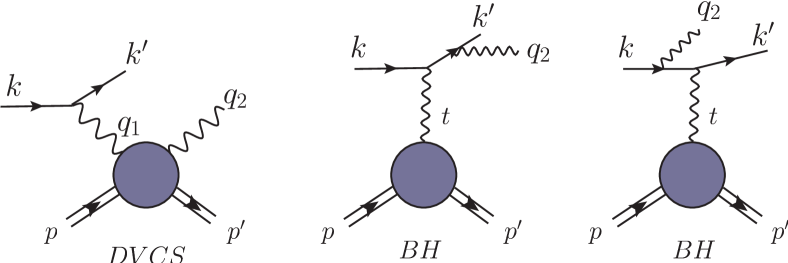
Figure 1: Amplitudes contributing to the photon leptoproduction cross section in leading order approximation of QED: the DVCS amplitude (left) while the remaining two diagrams (middle and right) represent the Bethe-Heitler amplitudes, parameterized by hadronic electromagnetic form factors.

Phenomenologically, exclusive electroproduction of a real photon, DVCS, diagrammatically depicted in Fig. 1 (left), is the golden channel to constrain GPDs as it is theoretically clean and the phase of its amplitude can be measured using the interference with the Bethe-Heitler (BH) amplitude (see Fig. 1 middle/right). Besides that, the measurement of Compton scattering observables, even at rather low photon virtuality, is important since it provides insight into the fundamental Compton scattering process in the virtual regime. Since the virtual Compton process contains twelve helicity amplitudes (or equivalently twelve complex Compton form factors (CFFs) Belitsky:2001ns ), their disentanglement is already an experimental challenge. The measurement of CFFs should be considered a primary task, as important as the measurement of electromagnetic nucleon form factors. In return, the (partial) disentanglement of the various CFFs offers then a phenomenologically much simpler and cleaner access to GPDs.

Based on present phenomenological GPD knowledge, Monte Carlo simulations, and GPD fitting routines, we explore in our studies here both the DVCS process and the access to the spatial transverse distribution of quarks and gluons at a proposed Electron-Ion Collider (EIC). The much more general physics case of this suggested high-luminosity collider with a dedicated detector for exclusive channels in the medium to high energy regime of lepton-nucleon and lepton-nuclei scattering is described in Accardi:2012hwp .

The rest of this article is organized as follows: in Sect. 2 we introduce the theory elements, needed for the access of GPDs from DVCS observables, including also, for the unpolarized case, the exact dependence of a (reduced) $t$-differential photon electroproduction cross section on the electron energy loss variable $y$. Furthermore, we give a short overview of existing DVCS measurements. In Sect. 3 we describe the planned EIC at its different stages and the Monte Carlo simulation technique used in the generation of EIC DVCS pseudo-data. In Sect. 4 we shortly introduce three GPD models which are then utilized to provide predictions for the $t$-differential DVCS cross section, single spin and lepton charge DVCS asymmetries at different EIC kinematics. In Sect. 5 we discuss the access of GPD $H$ and $E$ at the final stage of EIC by using the DVCS cross section and single transverse proton spin asymmetry. Furthermore, we quantify the implications of such measurements for the imaging of the proton and comment on the qualitative aspects of such measurements for the spin sum rule. Finally, we summarize and conclude in Sect. 6.

2 Deeply virtual Compton scattering

The differential photon electroproduction cross section is five-fold and consists of the sum of the BH amplitude squared, DVCS amplitude squared, and the interference (INT) terms, where the latter is charge odd:

$$\frac{d\sigma^{ep\to ep\gamma}}{dx_{\rm B}dtd{\cal Q}^{2}d\phi d\varphi}=\frac{d\sigma^{ep\to ep\gamma,\mbox{\tiny BH}}(F_{1},F_{2})}{dx_{\rm B}dtd{\cal Q}^{2}d\phi d\varphi}\pm\frac{d\sigma^{ep\to ep\gamma,\mbox{\tiny INT}}(F_{1},F_{2},{\cal F})}{dx_{\rm B}dtd{\cal Q}^{2}d\phi d\varphi}+\frac{d\sigma^{ep\to ep\gamma,\mbox{\tiny(D)VCS}}({\cal F},{\cal F}^{\ast})}{dx_{\rm B}dtd{\cal Q}^{2}d\phi d\varphi}\,.$$ (1)

Here the $+(-)$ sign is valid for electron (positron) beam, $x_{\rm B}$ is the common Bjorken scaling variable, $\phi$ is the azimuthal angle between lepton and hadron scattering planes, and $\varphi=\Phi-\phi$, where $\Phi(\equiv\phi_{S})$ is the angle between the lepton scattering plane and a possible transverse spin component of the incoming proton at rest. We adopt in the following the frame conventions of Belitsky:2001ns (virtual photon momentum is counter-along the $z$-direction and $x$-component of the incoming electron momentum is positive). To the leading order (LO) in the electromagnetic fine structure constant $\alpha_{\rm em}=\frac{e^{2}}{4\pi}\approx\frac{1}{137},$ and neglecting the electron mass, the three terms on the r.h.s. of (1) are exactly known in terms of the electromagnetic Pauli form factor $F_{1}(t)$ and the Dirac form factor $F_{2}(t)$, parameterizing the BH amplitude, and a set of twelve photon helicity dependent CFFs ${\cal F}_{ab}(x_{\rm B},t,{\cal Q}^{2})$, parameterizing the DVCS amplitude, see Fig. 1. These CFFs are labeled by the helicities of the incoming $a\in\{+,0,-\}$ and outgoing photon $b\in\{+,-\}$ and they are called

$${\cal F}_{ab}\in\{{\cal H}_{ab},{\cal E}_{ab},\widetilde{\cal H}_{ab},\widetilde{\cal E}_{ab}\}\quad\mbox{with}\quad{\cal F}_{0-}={\cal F}_{0+}\,,\quad{\cal F}_{+-}={\cal F}_{-+}\,,$$ (2)

more details can be found in Belitsky:2010jw ; Belitsky:2012ch . Analogously to the Dirac and Pauli form factor $F_{1}$ and $F_{2}$ (axial and pseudo-scalar form factors $F_{A}$ and $F_{P}$), the CFFs ${\cal H}(\widetilde{\cal H})$ and ${\cal E}(\widetilde{\cal E})$ ) are associated with conserved proton helicity amplitudes and helicity flipped ones, respectively.

The three separate terms of the differential electroproduction cross section (1) can be expanded w.r.t. harmonics of the azimuthal angle $\phi$,

$$\frac{d\sigma^{ep\to ep\gamma,\mbox{\tiny BH}}(F_{1},F_{2})}{dx_{\rm B}dtd{\cal Q}^{2}d\phi d\varphi}=\frac{\alpha_{\rm em}^{3}}{16\,\pi^{2}\,{{\cal Q}}^{4}}\,\frac{x_{\rm B}^{-1}(1+\epsilon^{2})^{-5/2}}{t\,{\cal P}_{1}(\phi,y){\cal P}_{2}(\phi,y)}\left\{\sum_{n=0}^{2}c^{\mbox{\tiny BH}}_{n}\cos{(n\phi)}+s^{\mbox{\tiny BH}}_{1}\sin{(\phi)}\!\right\},\\$$ (3)

$$\frac{d\sigma^{ep\to ep\gamma,\mbox{\tiny INT}}(F_{1},F_{2})}{dx_{\rm B}dtd{\cal Q}^{2}d\phi d\varphi}=\frac{\alpha_{\rm em}^{3}}{16\,\pi^{2}\,{{\cal Q}}^{4}}\,\frac{y^{-1}(1+\epsilon^{2})^{-1/2}}{t{\cal P}_{1}(\phi,y){\cal P}_{2}(\phi,y)}\left\{\!c^{\mbox{\tiny INT}}_{0}+\sum_{n=1}^{3}\left[c_{n}^{\mbox{\tiny INT}}\cos(n\phi)+s_{n}^{\mbox{\tiny INT}}\sin(n\phi)\right]\!\right\},\\$$ (4)

$$\frac{d\sigma^{ep\to ep\gamma,\mbox{\tiny VCS}}({\cal F},{\cal F}^{\ast})}{dx_{\rm B}dtd{\cal Q}^{2}d\phi d\varphi}=\frac{\alpha_{\rm em}^{3}}{16\,\pi^{2}\,{{\cal Q}}^{4}}\,\frac{x_{\rm B}(1+\epsilon^{2})^{-1/2}}{{\cal Q}^{2}}\left\{\!c^{\mbox{\tiny VCS}}_{0}+\sum_{n=1}^{2}\left[c^{\mbox{\tiny VCS}}_{n}\cos(n\phi)+s^{\mbox{\tiny VCS}}_{n}\sin(n\phi)\right]\!\right\}.$$ (5)

Here $1/({\cal P}_{1}(\phi,y){\cal P}_{2}(\phi,y))$ are (rescaled) BH propagators, defined in (32) of Belitsky:2001ns , the energy loss

$$y=\frac{1}{x_{\rm B}}\frac{{\cal Q}^{2}}{s-M_{p}^{2}}$$ (6)

of the electron depends for fixed $x_{\rm B}$ and ${\cal Q}^{2}$ on the center-of-mass (c.o.m.) energy squared $s$, and, finally, we used the shorthand $\epsilon\equiv 2x_{\rm B}M_{p}/{\cal Q}$. Moreover, all of the Fourier coefficients $c_{n}^{\cdots}$ and $s_{n}^{\cdots}$ depend on the polarization vectors of the protons. The explicit expressions for an incoming polarized nucleon has been presented in Belitsky:2012ch , where for transverse polarization the coefficients can be further decomposed in $\cos(\varphi)$ and $\sin(\varphi)$ harmonics. Note that if one reduces the five-fold cross section (1) to a four-fold one by integrating over $\varphi$, the $\varphi$-harmonics drop out and the remaining unpolarized and longitudinally polarized parts of the expressions (3–5) are multiplied by a factor $2\pi$. The knowledge of the coefficients in the BH term (3) is limited only by the knowledge of the proton form factors $F_{1}(t)$ and $F_{2}(t)$. The coefficients of the interference (4) and (D)VCS term (5) are linear and bi-linear in the CFFs, respectively. We emphasize that electromagnetic corrections will enter in all three terms. So far such $\alpha_{\rm em}/\pi$-proportional corrections are only partially taken into account in radiative correction procedures.

Adopting the discussion of Belitsky:2001ns , we can state that an over-complete set of observables exist and that at least in principle their experimental measurements would allow to extract the real and imaginary parts of all twelve CFFs (2). Loosely speaking, in the deeply virtual regime the first harmonics in the interference term are dominant, i.e., proportional to $1/{\cal Q}^{3}$, and are governed by twist-two associated CFFs (or GPDs), while the constant and second harmonics are kinematical suppressed by $1/{\cal Q}$ and arise in leading order of perturbative QCD from both twist-two and twist-three associated CFFs (or GPDs). The third harmonics are counted as leading twist contributions, however, they arise in next-to-leading order (NLO) of perturbative QCD from gluon transversity GPDs. A rather analogous counting scheme holds for the zeroth, first, and second harmonics of the DVCS term, where, compared to the interference term, an additional kinematical factor $1/{\cal Q}$ appears. Because of this mismatch in twist and power counting, some care is needed.

In the rest of this Sect. 2 we consider: in Sect. 2.1, the $y$-dependence of the $\phi$-integrated electroproduction cross section (1) for an unpolarized proton and in Sect. 2.2 we point out that the relation of helicity CFFs to GPDs can be systematically improved. In Sect. 2.3 we give a short overview of existing DVCS measurements and make a loose contact to CFF/GPD phenomenology.

2.1 Rosenbluth separation of electroproduction cross section

It would be very desirable to decompose the photon electroproduction cross section (1) into its different parts (3–5). In an experimental setup in which both electrons and positrons are available, the charge-odd interference term (4) and the charge-even part, given as sum of BH and DVCS cross sections (3,5), can be obviously separated from each other by forming the difference and sum of electron and positron cross sections. Having only an electron beam at hand, it remains so far unclear to what extent a variation of c.o.m. energy (or electron/proton beam energy) allows for a Rosenbluth separation, which is expected to be much more intricate than in the case of elastic form factors or deeply inelastic scattering (DIS) structure functions. We recall that in these cases two form factor combinations (or structure functions) enter the unpolarized cross sections; however, both of them arise from transversely or longitudinally polarized photon exchanges and are thus accompanied with a different $y(x_{\rm B},{\cal Q}^{2},s)$ dependence, which varies for fixed $x_{\rm B}$ and ${\cal Q}^{2}$ with the c.o.m. energy $\sqrt{s}$, see (6), i.e., with the beam energy (or energies).

Having the exact analytic expressions of Belitsky:2012ch in mind, it looks hopeless to employ a Rosenbluth separation directly to the five-fold (or four-fold) cross section (1). Thus, it is more appropriate to project first on the azimuthal angle harmonics, where, however, the $\phi$- and $y$-dependencies of the BH propagators should be treated in such a way that the final result is most appropriate for the analyzes of experimental data. Including these propagators in the integral, as done in Belitsky:2001ns , provides a truncated Fourier series and allows for a rather simple power counting scheme; however, these Fourier coefficients will not have a simple $y$-dependence. Alternatively, one may stick to the standard Fourier coefficients, e.g., calculated from

$$\int_{-\pi}^{\pi}\!d\phi\,\cos{(n\phi)}\,\frac{d\sigma^{ep\to ep\gamma}}{dx_{\rm B}dtd{\cal Q}^{2}d\phi}\quad\mbox{for}\quad n=0,1,2,3,\cdots,$$ (7)

where the DVCS cross section only contributes to the first three lowest coefficients. In the following we will first consider only the lowest harmonic, i.e., $n=0$, which has a surprisingly simple and obvious $y$-dependence.

Let us first introduce a formally defined $t$-differential “photoproduction” cross section. It is obtained by integrating the four-fold electroproduction cross section over the azimuthal angle $\phi$, multiplying it with an infinitesimal electron phase space element, and dividing it by a flux factor,

$$\frac{d\sigma^{\mbox{\tiny TOT}}(x_{\rm B},t,{\cal Q}^{2}|y)}{dt} \equiv \frac{1}{\Gamma(x_{\rm B},{\cal Q}^{2}|y)}\int_{-\pi}^{\pi}\!d\phi\,\frac{d\sigma^{ep\to ep\gamma}(x_{\rm B},t,{\cal Q}^{2}|y)}{dtd\phi dx_{\rm B}d{\cal Q}^{2}}\times dx_{\rm B}d{\cal Q}^{2}$$

$$= \frac{d\sigma^{\mbox{\tiny\rm BH}}(x_{\rm B},t,{\cal Q}^{2}|y)}{dt}\pm\frac{d\sigma^{\mbox{\tiny\rm INT}}(x_{\rm B},t,{\cal Q}^{2}|y)}{dt}+\frac{d\sigma^{\mbox{\tiny\rm DVCS}}(x_{\rm B},t,{\cal Q}^{2}|y)}{dt}\,,$$

where as before the positive (negative) sign of the interference term refers to an electron (positron) beam. For the virtual photon flux we adopt the Hand convention Hand:1963bb by taking

$$\Gamma(x_{\rm B},{\cal Q}^{2}|y)=\frac{\alpha_{\rm em}}{2\pi}\frac{y^{2}}{1-\varepsilon(y)}\frac{1-x_{\rm B}}{x_{\rm B}{\cal Q}^{2}}\quad\mbox{with}\quad\varepsilon(y)=\frac{1-y-\frac{\epsilon^{2}y^{2}}{4}}{1-y+\frac{y^{2}}{2}+\frac{\epsilon^{2}y^{2}}{4}}$$ (9)

where $\varepsilon(y)$ is the ratio of longitudinal and transverse photon flux.

The $y$-dependence of the three terms in (2.1) and the explicit expressions for the Fourier coefficients can be evaluated from (3–5) . Thereby, the DVCS cross section is the most simplest one and given by the constant harmonic in (5), which is further specified in (36) of Belitsky:2012ch . The BH cross section can also be analytically calculated, where due to the $\phi$-dependence of the BH propagators also higher $\phi$ harmonics that arise from the interference of photon helicity flip amplitudes, specified in (35-37) of Belitsky:2001ns , enter. Thereby, the integration over the azimuthal angle $\phi$ generates a characteristic $y$-dependent function that stems from the product $1/({\cal P}_{1}(\phi,y){\cal P}_{2}(\phi,y))$ of BH propagators. Consequently, this function inherits the $u$-channel pole of one BH propagator at

$$y=y_{\rm col}\quad\mbox{with}\quad y_{\rm col}=\frac{{\cal Q}^{2}+t}{{\cal Q}^{2}+x_{\rm B}t}\,,$$

where the real photon and incoming electron momenta are collinear. In the following we present results for the region $y<y_{\rm col}$, in which this characteristic function reads:

$$\frac{1}{\left[1+\frac{t}{{\cal Q}^{2}}-y\frac{t}{{\cal Q}^{2}}(1-x_{\rm B})\right]\left[1+\frac{t}{{\cal Q}^{2}}-y\left(1+\frac{x_{\rm B}t}{{\cal Q}^{2}}\right)\right]}=\frac{\left(1+\frac{x_{\rm B}t}{{\cal Q}^{2}}\right)^{-1}}{\left[1+\frac{t}{{\cal Q}^{2}}-y\frac{t}{{\cal Q}^{2}}(1-x_{\rm B})\right]\left[y_{\rm col}-y\right]}.$$ (10)

The interference term is the most intricate one, since various CFF combinations, which have different $y$-dependencies, enter in the harmonics and due to the BH propagators all of them will contribute to the $\phi$-integrated interference term. Utilizing the exact results, given in (66,67,69) and appendix B.1 of Belitsky:2012ch , it can be shown that due to the $\phi$ integration the transverse CFFs ${\cal F}_{-+}$ disappear. Moreover, the $y$-dependent factor (10), arising from the BH propagators, cancel exactly in all remaining expressions and we also find a unique $y$-dependence for the net result. We also emphasize that the dominant first harmonic gets suppressed by $1/{\cal Q}$ and cancels a contribution in the constant term, yielding a result that is proportional to $x_{\rm B}^{2}$. Finally, we add that the CFFs $\widetilde{\cal E}_{++}$ and $\widetilde{\cal E}_{0+}$ are absent in the unpolarized interference term.

Let us skip here further details and quote the new results for the moderate/small-$x_{\rm B}$ region:

$$\frac{d\sigma^{\rm BH}}{dt}=\frac{4\pi\alpha_{\rm em}^{2}y^{2}}{-t{\cal Q}^{2}(1+\epsilon^{2})}\,\frac{\left[1-\frac{2x_{\rm B}t}{{\cal Q}^{2}-t}\,\varepsilon(y)\right]\frac{(-1)\widetilde{K}^{2}({\cal Q}^{2}-t)}{t({\cal Q}^{2}+t)(1-x_{\rm B})}\left[F_{1}^{2}(t)-\frac{t}{4M_{p}^{2}}F_{2}^{2}(t)\right]+{\cal O}(x_{\rm B}^{2})}{\left[1+\frac{t}{{\cal Q}^{2}}-y\frac{t}{{\cal Q}^{2}}(1-x_{\rm B})\right]\left[1+\frac{t}{{\cal Q}^{2}}-y\left(1+\frac{x_{\rm B}t}{{\cal Q}^{2}}\right)\right]},\\$$ (11)

$$\frac{d\sigma^{\mbox{\tiny\rm INT}}}{dt}=\frac{4\pi\alpha_{\rm em}^{2}\,y(2-y)}{{\cal Q}^{4}(1+\epsilon^{2})(2-2y+y^{2}+\frac{\epsilon^{2}y^{2}}{2})}\;\frac{x_{\rm B}^{2}}{1-x_{\rm B}}\Re{\rm e}\,{\cal C}({\cal F}_{++}|{\cal F}_{0+})\,,\phantom{\Bigg{|}}\\$$ (12)

$$\frac{d\sigma^{\mbox{\tiny\rm VCS}}}{dt}=\frac{\pi\alpha_{\rm em}^{2}}{{\cal Q}^{4}\sqrt{1+\epsilon^{2}}}\,\frac{x_{\rm B}^{2}}{1-x_{\rm B}}\left[{\cal C}({\cal F}_{++},{\cal F}_{++}^{\ast})+{\cal C}({\cal F}_{-+},{\cal F}_{-+}^{\ast})+\varepsilon(y)\,{\cal C}({\cal F}_{0+},{\cal F}^{\ast}_{0+})\right],$$ (13)

where the bi-linear ${\cal C}$-coefficient of the (D)VCS term is given in (45) of Belitsky:2012ch and the linear ${\cal C}$-coefficient of the interference term reads

$${\cal C}({\cal F}_{++}|{\cal F}_{0+})=\left[F_{1}(t){\cal H}_{++}-\frac{t}{4M^{2}}F_{2}(t){\cal E}_{++}-\left\{F_{1}(t)+F_{2}(t)\right\}\widetilde{\cal H}_{++}\right]\!(x_{\rm B},t,{\cal Q}^{2})+{\cal O}(x_{\rm B})\,.$$ (14)

Note that here the longitudinal helicity CFFs are suppressed by an additional $x_{\rm B}$ factor. From the equations (11-13) one immediately reads off the well-known canonical scaling and the characteristic $y$ hierarchy of the BH, interference, and DVCS term, given by

$$\frac{d\sigma^{\mbox{\tiny BH}}}{dt}\propto\frac{y^{2}}{-t{\cal Q}^{2}}\,,\qquad\frac{d\sigma^{\mbox{\tiny INT}}}{dt}\propto\frac{y}{{\cal Q}^{4}}\,,\quad\mbox{and}\quad\frac{d\sigma^{\mbox{\tiny DVCS}}}{dt}\propto\frac{1}{{\cal Q}^{4}}\,,$$

respectively. A few further comments about the variable dependencies are in order.

• $y$-dependencies

The power behavior in $y$ of the BH, interference, and DVCS term is modified. More precisely, we have for these three terms the hierarchy

$$\frac{y^{2}}{\left[1+\frac{t}{{\cal Q}^{2}}-y\frac{t}{{\cal Q}^{2}}(1-x_{\rm B})\right]\left[1+\frac{t}{{\cal Q}^{2}}-y\left(1+\frac{x_{\rm B}t}{{\cal Q}^{2}}\right)\right]}\,,\qquad\frac{y(2-y)}{2-2y+y^{2}+\frac{\epsilon^{2}y^{2}}{2}}\,,\qquad 1,$$ (15)

where both the BH and DVCS term is further separated into transverse and longitudinal parts. The latter is proportional to the polarization parameter $\varepsilon(y)$, which, however, in DVCS kinematics appears to be power suppressed. The additional $y$-dependence of the BH term, cf. (10), depends on both the $t/{\cal Q}^{2}$ ratio and $x_{\rm B}$. At $y=0$ and in the vicinity of $y_{\rm col}$ it has the values

$$\frac{1}{\left(1+\frac{t}{{\cal Q}^{2}}\right)^{2}}\sim 1\quad\mbox{and}\quad\frac{1}{\left(1+\frac{t}{{\cal Q}^{2}}\right)\left(1-\frac{t}{{\cal Q}^{2}}+\frac{2x_{\rm B}t}{{\cal Q}^{2}}\right)}\,\frac{1}{y_{\rm col}-y}\sim\frac{1}{1-y}\,,$$ (16)

respectively. In the DVCS kinematics this function can be approximated by $1/(1-y)$. The additional $y$-dependence of the interference term (12) is given by the rather mild concave function

$$\frac{2-y}{2-2y+y^{2}+\frac{\epsilon^{2}y^{2}}{2}}\approx\frac{2-y}{2-2y+y^{2}}\,,$$

which takes the value one at both endpoints $y\in\{0,\approx\!\!1\}$ and has a maximum of $\approx 1.21$ at $y\approx 0.59$.

• $t$-dependence of the BH cross section

The kinematical factor $\widetilde{K}^{2}/(-t)$ in the BH cross section (11) is proportional to $(t-t_{\rm min})/t$ and, hence, it vanishes at the phase space boundary $t\to t_{\rm min}$. Thereby, the BH cross section (11) remains finite and is proportional to $x_{\rm B}^{2}/(-t_{\rm min})$. If we have the region $-t_{\rm min}\ll-t$ in mind, where $-t_{\rm min}\sim x_{\rm B}^{2}M_{p}^{2}$ vanishes at small $x_{\rm B}$, we will loosely say that the BH cross section is proportional to $1/(-t)$. We add that in this $t$-region and for $x_{\rm B}\lesssim 0.05$ the approximation (11) works on the level of one percent and better.

• small-$x_{\rm B}$ region

At small $x_{\rm B}$ the CFF behavior is governed by a possible “pomeron” exchange, which yields that even $x_{\rm B}\times{\cal F}(x_{\rm B},t,{\cal Q}^{2})$ may grow for decreasing $x_{\rm B}$ values. Taking the limit $x_{\rm B}\to 0$ for the kinematical factors of (11–13) yields for $-t_{\rm min}\ll-t$ the rather accurate kinematic expressions

$$\frac{d\sigma^{\rm BH}}{dt} \!\approx\! \frac{4\pi\alpha_{\rm em}^{2}}{-t{\cal Q}^{2}}\;\frac{y^{2}\left[F_{1}^{2}(t)-\frac{t}{4M_{p}^{2}}F_{2}^{2}(t)\right]}{\left[y_{\rm col}-y\right]\left[1+(1-y)\frac{t}{{\cal Q}^{2}}\right]}\quad\mbox{for}\quad y<y_{\rm col}\approx 1+\frac{t}{{\cal Q}^{2}}\sim 1,$$ (17)

$$\frac{d\sigma^{\rm DVCS}}{dt} \!\approx\! \frac{\pi\alpha_{\rm em}^{2}}{{\cal Q}^{4}}x_{\rm B}^{2}\left[{\cal C}({\cal F}_{++},{\cal F}_{++}^{\ast})+{\cal C}({\cal F}_{-+},{\cal F}_{-+}^{\ast})+\varepsilon(y)\,{\cal C}({\cal F}_{0+},{\cal F}^{\ast}_{0+})\right],$$ (18)

where

$$x_{\rm B}^{2}\,{\cal C}({\cal F},{\cal F}^{\ast})\approx\left[\left|x_{\rm B}{\cal H}\right|^{2}-\frac{t}{4M^{2}_{p}}\left|x_{\rm B}{\cal E}\right|^{2}+\left|x_{\rm B}\widetilde{\cal H}\right|^{2}-\frac{t}{4M^{2}_{p}}\left|x_{\rm B}\overline{\cal E}\right|^{2}\right]\!\left(x_{\rm B},t,{\cal Q}^{2}\right)$$ (19)

with the new notation

$$\overline{\cal E}(x_{\rm B},t,{\cal Q}^{2})\approx\frac{x_{\rm B}}{2-x_{\rm B}}\widetilde{\cal E}(x_{\rm B},t,{\cal Q}^{2})\,.$$ (20)

The interference term is suppressed w.r.t. DVCS cross section by an additional factor $x_{\rm B}\,y$ and can be safely neglected. As one immediately realizes from these rather accurate kinematic approximations, the BH cross section (17) is kinematically enhanced at small $-t$ and suppressed at small $y$ values. However, most important is that the DVCS cross section (18) in the small-$x_{\rm B}$ region grows with decreasing $x_{\rm B}$, caused by an effective “pomeron” exchange in the $t$-channel. Thus, even the relative kinematical $-t(1-y)/{\cal Q}^{2}y^{2}$ suppression of the DVCS cross section w.r.t. BH one can be overcome. Moreover, the DVCS signal can be further experimentally enhanced by an upper $y$ cut. However, it should be kept in mind that the ratio of DVCS cross section to the BH one depends on the competing interplay of $x_{\rm B}$, ${\cal Q}^{2}$, and $t$ dependencies. In particular, if the DVCS cross section falls off much faster with increasing $-t$ than the electromagnetic form factor $F_{1}(t)$, like in the case of the often assumed exponential $t$-dependence, the ratio of DVCS cross section to BH one can become very small at larger $-t$ values.

Finally, let us quote the $y$-dependence of the $t$-differential cross section (2.1) in the most obvious manner for general DVCS kinematics ${\cal Q}^{2}>-t$ and $y<y_{\rm col}$:

$$\frac{d\sigma^{\mbox{\tiny TOT}}}{dt}=\frac{y^{2}\left[\frac{d\sigma_{\rm T}^{\mbox{\tiny BH}}}{dt}+\varepsilon(y)\frac{d\sigma_{\rm L}^{\mbox{\tiny BH}}}{dt}\right]}{\left(1-y\frac{(1-x_{\rm B})t}{{\cal Q}^{2}+t}\right)\left(\frac{{\cal Q}^{2}+t}{{\cal Q}^{2}+x_{\rm B}t}-y\right)}\pm\frac{y\left(1-\frac{y}{2}\right)\sqrt{1+\epsilon^{2}}}{1-y+\frac{y^{2}}{2}+\frac{\epsilon^{2}y^{2}}{4}}\,\frac{d\sigma_{\rm T}^{\mbox{\tiny INT}}}{dt}+\frac{d\sigma_{\rm T}^{\mbox{\tiny DVCS}}}{dt}+\varepsilon(y)\frac{d\sigma_{\rm L}^{\mbox{\tiny DVCS}}}{dt}\,.$$ (21)

The reduced BH cross section $d\sigma_{\rm T}^{\mbox{\tiny BH}}/dt+\varepsilon(y)d\sigma_{\rm L}^{\mbox{\tiny BH}}/dt$ for the smaller-$x_{\rm B}$ region, the reduced interference term $d\sigma_{\rm T}^{\mbox{\tiny INT}}/dt$, and the DVCS cross section $d\sigma_{\rm T}^{\mbox{\tiny DVCS}}/dt+\varepsilon(y)d\sigma_{\rm L}^{\mbox{\tiny DVCS}}/dt$ can be read off from (11), (12), and (13), respectively. Note that the $y$-dependent factor in front of the interference term is given by a transverse photon flux asymmetry,

$$\frac{y\left(1-\frac{y}{2}\right)\sqrt{1+\epsilon^{2}}}{1-y+\frac{y^{2}}{2}+\frac{\epsilon^{2}y^{2}}{4}}=\frac{{\cal L}_{--}-{\cal L}_{++}}{{\cal L}_{--}+{\cal L}_{++}}.$$

Depending on the kinematics, the application of the formula (21) is two-fold. In the case that the subtraction of the BH cross section can be reliably done, the measurement of this subtracted cross section at three different beam energies allows in principle to separate the longitudinal DVCS cross section, transverse DVCS cross section, and the interference term. One may also utilize the $y$-dependence to cross-check experimentally if a BH-subtraction procedure is well understood.

2.2 Relating DVCS observables to GPDs

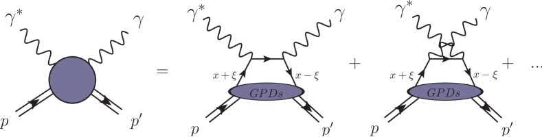
Figure 2: Factorization of the DVCS amplitude to leading order in perturbative QCD and to leading twist-two accuracy. This yields equation (24) that expresses CFFs (filled circle) in terms of GPDs (filled ellipse).

GPDs, denoted here generically as

$$F(x,\eta=\xi,t,\mu^{2})\quad\mbox{with}\quad F\in\{H,E,\widetilde{H},\widetilde{E}\}\,,$$

are intricate functions that, besides depending on the partonic momentum fraction $x$ and the momentum transfer squared $t$, depend also on the $t$-channel longitudinal momentum fraction $\eta$, called skewness (often denoted by $\xi$ in the literature), and on the factorization scale $\mu^{2}$. The unpolarized parton GPDs are called $H$ and $E$ Ji:1998pc , where the former (latter) GPD can be loosely associated with a proton helicity (non)conserved distribution. Analogous nomenclature is used for the polarized parton GPDs $\widetilde{H}$ and $\widetilde{E}$ Ji:1998pc . GPDs have certain spectral properties Mueller:1998fv ; Radyushkin:1997ki and so their $x$-moments are polynomials of certain order in $\eta$, with lowest moments being equal to elastic nucleon form factors. In the forward limit ($t\to 0$, $\eta\to 0$) $H$ ($\widetilde{H}$) reduce to the unpolarized (polarized) Parton Distribution Functions (PDFs), commonly called $(\Delta)q$ and $(\Delta)g$ for quarks and gluon, respectively. Furthermore, in the region $|x|>\eta$, where a parton is exchanged in the $s$-channel, GPDs are constrained by positivity conditions Martin:1997wy ; Pire:1998nw ; Radyushkin:1998es ; Ji:1998pc ; Diehl:2000xz , which can be viewed in their most general form as a consequence of a wave function overlap representation Pobylitsa:2002iu ; Pobylitsa:2002vw ; Pobylitsa:2002vi . However, this GPD property is exact only to LO accuracy. To our best knowledge, no attempt has been undertaken to derive positivity constraints for the $\eta=x$ case. This implies that existing positivity constraints mostly do not apply for the phenomenological description of deeply virtual processes. However, as we will see below, they are important constraints for GPD models, e.g., as used by us in Sect. 5.2 for the purpose of extrapolation from the $\eta=x$ to the $\eta=0$ case.

DVCS observables can be exactly evaluated in terms of the helicity CFFs (2). To express them in terms of GPDs in a systematically improvable manner, it is maybe appropriate to utilize a conventionally defined GPD-inspired CFF basis, such as the one introduced in Belitsky:2001ns :

$${\cal F}\in\{{\cal H},{\cal E},\widetilde{\cal H},\widetilde{\cal E},{\cal H}_{3},{\cal E}_{3},\widetilde{\cal H}_{3},\widetilde{\cal E}_{3},{\cal H}_{\rm T},{\cal E}_{\rm T},\widetilde{\cal H}_{\rm T},\widetilde{\cal E}_{\rm T}\}\,.$$ (22)

Here, the CFFs ${\cal H},{\cal E},\widetilde{\cal H}$, and $\widetilde{\cal E}$ are associated with twist-two GPDs $F\in\{H,E,\widetilde{H},\widetilde{E}\}$ and govern the photon helicity non-flip DVCS amplitude, i.e., at leading twist-two accuracy we have

$${\cal F}_{++}(x_{\rm B},t,{\cal Q}^{2})={\cal F}(x_{\rm B},t,{\cal Q}^{2})+{\cal O}(1/{\cal Q}^{2})\quad\mbox{for}\quad{\cal F}\in\{{\cal H},{\cal E},\widetilde{\cal H},\widetilde{\cal E}\}.$$ (23)

It is ensured by the factorization theorem Collins:1998be ; Radyushkin:1997ki ; Ji:1998xh that these four dominant CFFs arise from the convolution of twist-two GPDs with hard coefficients, which are perturbatively calculable as a series in the strong coupling constant $\alpha_{s}$. Presently, these coefficients are known to NLO accuracy in the standard minimal subtraction scheme Belitsky:1997rh ; Mankiewicz:1997bk ; Ji:1997nk ; Ji:1998xh ; Belitsky:1999hf ; Pire:2011st and to next-to-next-to-leading order (NNLO) accuracy in a special scheme Mue05a ; KumMuePasSch06 . To LO they are calculated from the handbag diagram, depicted in Fig. 2, yielding the convolution formula

$${\cal F}(x_{\rm B},t,{\cal Q}^{2})\stackrel{{\scriptstyle\rm LO}}{{=}}\sum\limits_{i}\int_{-1}^{1}\!dx\left[\frac{e^{2}_{i}}{\xi-x-i\epsilon}\mp\{x\rightarrow-x\}\right]F_{i}(x,\xi,t,\mu^{2})\;\;\mbox{for}\;\;{\cal F}\in\left\{{{\cal H},{\cal E}\atop\widetilde{\cal H},\widetilde{\cal E}}\right\},$$ (24)

where $e_{i}$ are the fractional quark charges. The variable $\xi\sim x_{\rm B}/(2-x_{\rm B})$ is a conventionally defined Bjorken-like scaling variable, equated to the longitudinal momentum fraction in the $t$-channel, and $\mu^{2}\sim{\cal Q}^{2}$ being the factorization scale. Note the conventional dependence as function of this scaling variable is in the orders of $O(1/{\cal Q}^{2})$. It further reduces if one takes into account kinematic corrections, evaluated to twist-four accuracy at LO in $\alpha_{s}$ Braun:2011zr ; Braun:2011dg ; Braun:2012bg ; Braun:2012hq . As is well known, the ambiguity in setting the factorization scale diminishes in higher orders of perturbation theory as long as the perturbative corrections to the GPD evolution are consistently taken into account. Moreover, as long as we consider only the DVCS process, the perturbative order to which we describe its amplitude can be mainly understood as a convention (in a DVCS scheme, like in the DIS scheme, only the perturbatively predicted evolution would alter, if we would switch, e.g., from LO to NLO). In the minimal subtraction scheme the evolution kernels are known to NLO accuracy Belitsky:1999hf . We also recall the fact, well known from unpolarized DIS, that the absence of gluon GPDs in the LO convolution equations (24) does not imply that these GPDs are absent from a LO description; they drive the evolution of the sea quarks.

The CFFs ${\cal H}_{3},{\cal E}_{3},\widetilde{\cal H}_{3}$, and $\widetilde{\cal E}_{3}$ are expressed by twist-three GPDs, containing information on three-parton correlation functions, and enter into the photon helicity longitudinal-transversal flip amplitude, which reads to twist-three and LO in $\alpha_{s}$ accuracy as

$${\cal F}_{0+}(x_{\rm B},t,{\cal Q}^{2})=-\frac{\sqrt{2}\widetilde{K}}{{\cal Q}\sqrt{1+\epsilon^{2}}\left(2-x_{\rm B}+\frac{x_{\rm B}t}{{\cal Q}^{2}}\right)}\left[x_{\rm B}{\cal F}+{\cal F}_{3}\right](x_{\rm B},t,{\cal Q}^{2})+{\cal O}\left(1/{\cal Q}^{2}\right)+{\cal O}(\alpha_{s})\,,\quad$$ (25)

where

$$\widetilde{K}=\sqrt{-(1-x_{\rm B})\left(\!1+\frac{x_{\rm B}t}{{\cal Q}^{2}}\!\right)t-\left(\!1+\frac{t}{{\cal Q}^{2}}\!\right)^{2}x_{\rm B}^{2}M_{p}^{2}}$$ (26)

is a kinematical factor that vanishes at the minimal value of $-t$. The CFFs ${\cal H}_{\rm T},{\cal E}_{\rm T},\widetilde{\cal H}_{\rm T}$, and $\widetilde{\cal E}_{\rm T}$ are the dominant contributions to the transverse helicity flip DVCS amplitude, which, at leading twist accuracy, arises from the transversely polarized gluon GPDs that are perturbatively Belitsky:2000jk and power suppressed Kivel:2001rw ; Braun:2012bg ; Braun:2012hq . Consequently, we have

$${\cal F}_{-+}(x_{\rm B},t,{\cal Q}^{2})={\cal F}_{\rm T}(x_{\rm B},t,{\cal Q}^{2})+{\cal O}\left(1/{\cal Q}^{2}\right)\quad\mbox{with}\quad{\cal F}_{\rm T}(x_{\rm B},t,{\cal Q}^{2})={\cal O}(\alpha_{s})\,.$$ (27)

If not stated otherwise, in the following we work for convenience to twist-two and LO accuracy, where we take four light quarks and we adopt the conventions

$$\xi=\frac{x_{\rm B}}{2-x_{\rm B}}\quad\mbox{and}\quad\mu^{2}={\cal Q}^{2}\,.$$ (28)

With these approximations GPD phenomenology can be drastically simplified. Namely, the convolution formula (24) tells us that the imaginary parts of the four dominant CFFs are given by the GPDs on the cross-over line $x=\xi$,

$$\Im{\rm m}{\cal F}(x_{\rm Bj},t,{\cal Q}^{2}) \stackrel{{\scriptstyle\rm LO}}{{=}} \pi F(\xi,\xi,t,{\cal Q}^{2})\,,\quad F\in\{H,E,\widetilde{H},\widetilde{E}\}\,.$$ (29)

Furthermore, by means of the GPD spectral property one obtains from (24) a dispersion integral representation for the real parts of these CFFs Teryaev:2005uj ,

$$\Re{\rm e}\!\left\{\!{\cal H}\atop{\cal E}\!\right\}\!(x_{\rm Bj},t,{\cal Q}^{2}) \stackrel{{\scriptstyle\rm LO}}{{=}} {\rm PV}\!\int_{0}^{1}\!dx\,\frac{2x}{\xi^{2}-x^{2}}\!\left\{\!H\atop E\!\right\}\!(x,x,t,{\cal Q}^{2})\mp{\cal C}(t,{\cal Q}^{2})\,,$$ (30)

$$\Re{\rm e}\!\left\{\!\widetilde{\cal H}\atop\widetilde{\cal E}\!\right\}\!(x_{\rm Bj},t,{\cal Q}^{2}) \stackrel{{\scriptstyle\rm LO}}{{=}} {\rm PV}\!\int_{0}^{1}\!dx\,\frac{2}{\xi^{2}-x^{2}}\!\left\{\!\xi\widetilde{H}\atop x^{2}\widetilde{E}\!\right\}\!(x,x,t,{\cal Q}^{2})+\frac{1}{\xi}\left\{\!0\atop\widetilde{\cal C}(t,{\cal Q}^{2})\!\right\}\,.$$ (31)

Here ${\cal D}=-{\cal C}$, entering in (30) as subtraction term, is given as convolution of the so called $D$-term contribution (introduced in Polyakov:1999gs to complete GPD polynomiality in one possible manner), which can be extracted for a given GPD. Note that the dispersion relation for $\widetilde{\cal E}$ is over-subtracted and that the subtraction constant $\widetilde{\cal C}(t,{\cal Q}^{2})$ contains a pion pole contribution. This pole contribution can be calculated rather analogously to the $D$-term, e.g., from the suggested parameterizations Mankiewicz:1998kg ; Frankfurt:1999xe or from extraction using a Regge-inspired GPD parametrization Bechler:2009me . Since in this approximated framework at fixed photon virtuality only the GPDs at the cross-over line $x=\xi$ and two subtraction constants enter, GPD phenomenology is drastically simplified.

2.3 Present status of DVCS measurements and GPD analyzes

Let us first consider experiments which have only an electron beam available. The three parts of the electroproduction cross section (1) contribute, depending on the kinematics, with different strength to the various harmonics. One can remove the BH cross section (3), taken to LO accuracy in $\alpha_{\rm em}$, by measuring the cross section differences for single spin flip observables, e.g., the beam-helicity difference $\Delta_{\rm LU}$

$$\frac{d\Delta_{\rm LU}}{dx_{\rm B}dtd{\cal Q}^{2}d\phi}=\frac{1}{2}\left[\frac{d\sigma^{\rightarrow}}{dx_{\rm B}dtd{\cal Q}^{2}d\phi}-\frac{d\sigma^{\leftarrow}}{dx_{\rm B}dtd{\cal Q}^{2}d\phi}\right],$$ (32)

and analogously for a longitudinally ($\Delta_{\rm UL}$) and transversely ($\Delta_{\rm UT}$) polarized proton target. These observables are expanded in terms of odd harmonics. In fixed target kinematics they are mainly dominated by the $\sin(\phi)$ and/or $\sin(\varphi)\cos(\phi)$ harmonics of the interference term (4), giving access to the imaginary part of four twist-two associated CFF combinations, see (47–50) below. However, the DVCS term (5), suppressed in these observables by $1/{\cal Q}^{2}$, may also contribute to some extent. We add that in double spin flip experiments the BH cross section (3) also enters, however its $\cos(\phi)$ harmonic can be quite small, which may allow the access to the $\cos(\phi)$ harmonic of the interference term, i.e., three combinations of twist-two associated CFF combinations.

Unpolarized electroproduction and electron-helicity dependent cross section measurements at rather large $x_{\rm B}$ and small $-t$ have been performed with small uncertainties by the Hall A collaboration at JLAB Munoz_Camacho:2006hx . The measured cross section differences (32) is compatible with various GPD model predictions, see Munoz_Camacho:2006hx ; Polyakov:2008xm ; Kroll:2012sm . In the unpolarized case, however, the measurements at four different $-t$ values, at ${\cal Q}^{2}=2.3\,\operatorname{GeV}^{2}$ and rather large $x_{\rm B}=0.36$ indicate that the DVCS cross section at these kinematics is much larger and drops much faster with growing $-t$ than expected from common GPD models. As explained in Sect. 2.1, at small $x_{\rm B}$ (large $W$) the “pomeron” behavior leads to the DVCS amplitude outgrowing the BH amplitude and as a result of the $\phi$-integration, the interference term is negligibly small in this region. Therefore, at the H1 Adloff:2001cn ; Aktas:2005ty ; Aaron:2007ab ; Aaron:2009ac and ZEUS Chekanov:2003ya ; Chekanov:2008vy collider experiments the DVCS cross section has been accessed by subtracting the BH cross section. Thereby, the subtraction method has been checked experimentally, since in some parts of the kinematic phase space the BH cross section dominates and Monte Carlo simulations can be directly confronted with measurements. The size of the cross section was predicted by a simple model FraFreStr98 and can be at NLO also described with standard GPD models, however, not at LO Freund:2001hd ; Guzey:2008ys . A simple flexible GPD model allows to describe the HERA collider data at LO, NLO, and NNLO, which allows to quantify GPD reparametrization effects Kumericki:2009uq .

In some experiments only asymmetries, less affected by possible normalization problems, are measurable. Having only an electron beam at hand one can access the interference term with single spin flip experiments by polarizing the electron beam longitudinally (electron beam-helicity asymmetry)

$$A_{\rm LU}=\left(\frac{d\sigma^{\rightarrow}}{dx_{\rm B}dtd{\cal Q}^{2}d\phi}-\frac{d\sigma^{\leftarrow}}{dx_{\rm B}dtd{\cal Q}^{2}d\phi}\right)\Big{/}\left(\frac{d\sigma^{\rightarrow}}{dx_{\rm B}dtd{\cal Q}^{2}d\phi}+\frac{d\sigma^{\leftarrow}}{dx_{\rm B}dtd{\cal Q}^{2}d\phi}\right),$$ (33)

and analogous equations hold true for single spin flip asymmetries with longitudinally ($A_{\rm UL}$) or transversely ($A_{\rm UT}$) polarized nucleons and unpolarized electron beams. Here, the squared BH term in the numerator will drop out again at LO accuracy in $\alpha_{\rm em}$ and the squared DVCS term will yield some contamination, while the normalization is governed by all three terms of the unpolarized cross section (1). In addition to longitudinal proton spin asymmetry measurements at HERMES Airapetian:2010ab and CLAS Chen:2006na , electron beam-helicity asymmetries were measured at CLAS Girod:2007aa ; Gavalian:2008aa .

The HERA experiments had both electrons and positrons beams available, which allowed to access the interference term via the beam charge asymmetry

$$A_{\rm C}=\left(\frac{d\sigma^{+}}{dx_{\rm B}dtd{\cal Q}^{2}d\phi}-\frac{d\sigma^{-}}{dx_{\rm B}dtd{\cal Q}^{2}d\phi}\right)\Big{/}\left(\frac{d\sigma^{+}}{dx_{\rm B}dtd{\cal Q}^{2}d\phi}+\frac{d\sigma^{-}}{dx_{\rm B}dtd{\cal Q}^{2}d\phi}\right),$$ (34)

where the numerator is entirely given by the interference term, however, the normalization depends also on the DVCS squared term. This asymmetry has been measured by the HERMES collaboration Airapetian:2006zr , where the correlation between the lowest and first harmonics, predicted in Belitsky:2001ns , was confirmed. The beam charge asymmetry was measured also by the H1 collaboration Aaron:2009ac at large $W$ (small $x_{\rm B}$) where, however, this observable (as well as the $t$-differential cross section and the longitudinal spin asymmetry) is dominated by the CFF $\cal H$ and uncertainties are large. Hence, the CFF $\cal E$, giving access to sea quark and gluon GPD $E$ that enters Ji‘s angular momentum sum rule, could not be revealed at small $x$.

The HERMES collaboration provided the most complete measurement of thirty-four DVCS asymmetries, where a missing-mass event selection method was employed. This includes also a partial interference/DVCS decomposition for asymmetries measured with a transversely polarized Airapetian:2008aa and unpolarized Airapetian:2009aa proton target. However, since the normalization depends on the unpolarized DVCS cross section and both statistical and systematical uncertainties are rather large, a full disentanglement of twist-two related CFFs and an access to the twist-three sector could not be achieved. In particular, GPD $E$ cannot be accessed from these measurements in a GPD model unbiased manner.

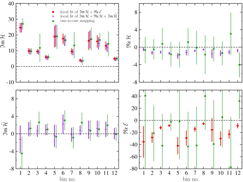
Figure 3: Results of least-squares fits in two scenarios with only a small number of CFFs locally fitted to data separately for each of 12 HERMES bins. First, with only $\Im{\rm m}\mathcal{H}$ and $\Re{\rm e}\mathcal{E}$ fitted (red diamonds) and, second, with $\Im{\rm m}\mathcal{H}$, $\Re{\rm e}\mathcal{H}$ and $\Im{\rm m}\widetilde{\mathcal{H}}$ (purple pluses). For comparison, result of a one-to-one mapping procedure is also shown (green stars).

This large set of DVCS observables, measured by HERMES in twelve kinematical bins (some are measured in 18 bins), allows for a local extraction of CFFs. Since experimental uncertainties are rather large for most of the observables, one may still rely on the hypothesis of twist-two dominance and extract the twist-two associated CFFs by maps Belitsky:2001ns , by least-squares fits Guidal:2008ie ; Guidal:2009aa ; Guidal:2010ig ; Guidal:2010de , or neural networks Kumericki:2011rz . To avoid a misinterpretation of experimental measurements, these local methods should be utilized with care. In particular, differences exist between the view points of random variable map and regression methods, see Fig. 3. A one-to-one map of eight twist-two dominated asymmetries into the space of CFFs reveals that only the imaginary part of the CFF $\cal H$ significantly differs from zero while its real part and the imaginary part of CFF $\widetilde{\cal H}$ are relative small. All other twist-two dominated CFFs have large uncertainties and are compatible with zero Kumericki:2013br . By means of the LO approximation (29) the results for the imaginary parts can now be viewed as GPDs on the cross-over line, while the dispersion relations (30, 31) may in principle be utilized as sum rules to constrain the GPDs on parts of the cross-over line that are outside of the accessible kinematics Kumericki:2008di . We add that so far no attempt has been made to access photon helicity flip contributions, related to twist-three and transversity GPDs. However, the smallness of higher harmonics is compatible with the hypothesis of twist-two dominance.

Certainly, the partonic interpretation of DVCS measurements, the inclusion of the ${\cal Q}^{2}$ evolution, perturbative corrections, kinematic corrections Braun:2011zr ; Braun:2011dg , and the access to three-parton correlations Belitsky:2000vx ; Belitsky:2001ns requires a global analysis with flexible GPD models. Having measurements over a wide ${\cal Q}^{2}$ range allows, through evolution, to reveal the GPD away from the cross-over line. This is used for the description of the DVCS cross section measurements at small $x_{\rm B}$, whereas for fixed target kinematics the ${\cal Q}^{2}$ lever arm is small and evolution effects are relatively weak (for an example study see Kumericki:2011zc ).

In a first step of a global DVCS analysis, unpolarized proton data were employed in GPD fits Kumericki:2009uq ; KumMueWeb ; Kumericki:2011zc . Thereby, the world data set could be described with $\chi^{2}/{\rm d.o.f.}\approx 1$, using the KM10 model. Nevertheless, in such a fit the four CFFs ${\cal H},{\cal E},\widetilde{\cal H},\widetilde{\cal E}$ cannot be disentangled and, partially for this reason, even the dominant ${\cal H}$ suffers from larger uncertainties, see Fig. 4. Below we will also employ the model KM10a, which has also a good $\chi^{2}/{\rm d.o.f.}\approx 1$ fit to the data set, but ignores the Hall A cross section measurements. Including polarized proton data in a global fit could certainly help to disentangle CFFs even better. In a more recent fit, given in Kumericki:2013br , we found that the KM model, designed for the unpolarized case, describes even such a set of DVCS data with $\chi^{2}/{\rm d.o.f.}\approx 1.6$, where most of the tension is due to the four unpolarized cross section measurements of Hall A collaboration. We emphasize that this tension can have different origins, e.g., it is maybe prudent to still consider the possibility that the experimental issue of exclusivity plays a role in most of the world data. For instance, beam spin asymmetry measurements from the HERMES collaboration with a complete event reconstruction yields an increase of their size, softening, thereby, the tension between measurements and standard GPD predictions Airapetian:2012pg ; Kroll:2012sm . ¿From present DVCS data, we can certainly state that GPD $H$ plays the dominant role, some phenomenological constraints for GPD $\widetilde{H}$ can be obtained, and proton helicity flip GPDs $E$ and $\widetilde{E}$ remain unconstrained. Let us add that present GPD phenomenology includes also deeply virtual meson production, in first place in the hand-bag model approach Goloskokov:2007nt ; Goloskokov:2008ib ; Goloskokov:2009ia ; Goloskokov:2011rd and was started in the perturbative factorization framework with flexible GPD models Bechler:2009me ; Meskauskas:2011aa . So far a reasonable description of the considered deeply virtual meson production channels and DVCS, currently explored on the level of LO accuracy, can be reached Kumericki:2011zc ; Meskauskas:2011aa ; Kroll:2012sm except for the large-$x_{\rm B}$ region.

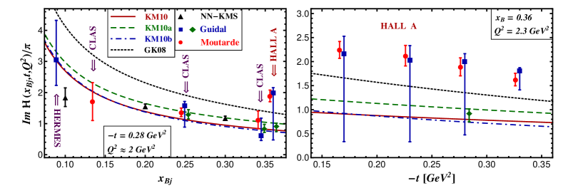
Figure 4: $\Im{\rm m}{\cal H}/\pi$ obtained from DVCS observables with different strategies: hybrid model fits KM10 (solid) KM10a (dashed), KM10b (dash-dotted) [Hall A cross section data are neglected], GK07 model from DVEM (dotted) Goloskokov:2007nt , seven-fold CFF fit Guidal:2008ie ; Guidal:2009aa with boundary conditions (squares), $\cal H$, $\widetilde{\cal H}$ CFF fit Guidal:2010ig (diamonds), smeared conformal partial wave model fit Moutarde:2009fg within $H$ GPD (circles). The triangles result from neural network fit Kumericki:2011rz .

As pointed out and illustrated in Figs. 3 and 4, present DVCS measurements provide some limited information on GPDs and future precision measurements are required to pin them down. New fixed target experiments are planned at COMPASS-II with a polarized muon beam, extending the HERMES kinematics to lower $x_{\rm B}$, and JLAB-12 GeV will bridge the gap between the kinematics of the present JLAB experiments’ to the HERMES experiment, see Fig. 5. Moreover, a high luminosity machine in the collider mode with polarized electron and proton or ion beams has been proposed Accardi:2012hwp and will be introduced in the next Section.

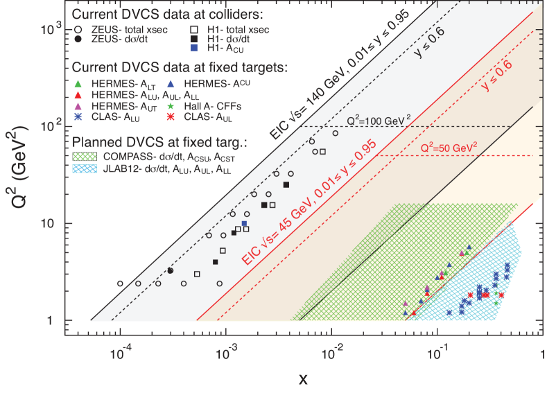
Figure 5: The kinematic reach in $x-{\cal Q}^{2}$ for existing DVCS measurements from H1/ZEUS, HERMES, CLAS and Hall A, as well as planned ones at COMPASS II and JLAB@12GeV, and the proposed EIC.

3 The EIC project and Monte Carlo simulation

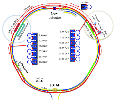
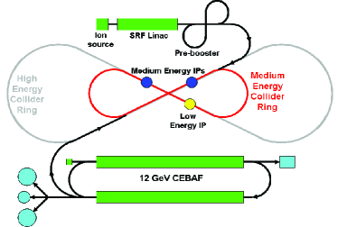
Figure 6: The Layout of the two proposed EIC machines: eRHIC (left) and ELIC (right).

In order to open a new window into a kinematic regime that allows the systematic study of quarks and gluons, EIC is designed to provide a wide range in c.o.m. energies, polarized lepton and light ions beams and heavy ion beams, all at a very high luminosity Accardi:2012hwp . This creates an unprecedented opportunity for discovery and precision measurements, and would allow us to study the momentum and space-time distribution of gluons and sea quarks in nucleons and nuclei EIC11 ; Accardi:2012hwp . The main requirements for an EIC machine are:

• Highly polarized ($>70\%$) electron and proton/light ion beams;

• Ion beams from deuteron to heaviest nuclei (uranium, lead);

• Variable center of mass energy, ranging from about $20\operatorname{GeV}$ up to $150\operatorname{GeV}$;

• Collision luminosity $\sim 10^{33-34}\,{\rm cm}^{-2}{\rm s}^{-1}$.

Two independent designs for a future EIC have evolved, eRHIC and ELIC, both using part of already available infrastructure and facilities (see chapter 5 in Accardi:2012hwp ). At Brookhaven National Laboratory (BNL) the eRHIC design (Figure 6 left) utilizes a new electron beam facility based on an Energy Recovery LINAC (ERL) to be built inside the RHIC tunnel to collide with RHICs high-energy polarized proton and nuclear beams. At JLAB the ELIC design (Figure 6 right) employs a new electron and ion collider ring complex together with the $12\operatorname{GeV}$ upgraded CEBAF, now under construction, to achieve similar collision parameters. The kinematic phase space achievable at an EIC for electron-proton collisions is shown in Fig. 5 and compared to existing DVCS data and planned future experiments. At an EIC it will be possible to study DVCS measuring, for the first time simultaneously and with high accuracy, both differential cross section and spin and charge asymmetries in a kinematic range that extends from large $x_{\rm B}$, typical for fixed target experiments, down to small $x_{\rm B}$, typical for the HERA collider experiments.

The present study is based on the eRHIC version of an EIC and its new dedicated detector, designed to fulfill the requirements for the golden experiments at an EIC and thus being simultaneously highly efficient for inclusive, semi-inclusive and exclusive reactions. The eRHIC expected luminosity for $ep$ collisions as a function of the beam-energy is shown in Figure 7. At eRHIC the full range of proton-beam energies will be at hand from the early beginning of operations, whereas the energy of the new electron-beam will be initially at $5-10\operatorname{GeV}$ (stage I) and will be later upgraded to higher energies up to $20-30\operatorname{GeV}$ (stage II). The newly designed eRHIC detector, shown in Fig. 7, will have the following properties:

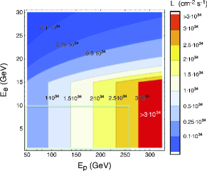
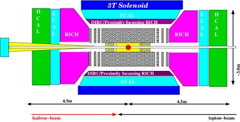
Figure 7: Left: the expected luminosity at the eRHIC collider as a function of the beam-energy configuration for $ep$ collisions. Right: a sketch of the eRHIC detector.

• Wide acceptance $-5<\eta<5$ for both the scattered lepton and the produced hadrons;

• The same rapidity coverage in electromagnetic calorimetry and tracking;

• High electron track finding/reconstruction efficiency, capability to discriminate two electromagnetic clusters down to a difference of $1$ degree of polar angle in the rear endcap electromagnetic calorimeter and good precision for momentum (energy) reconstruction;

• Particle identification to separate electrons and hadrons as well as pions, kaons and protons over a momentum range of $0.5\operatorname{GeV}$ to $10\operatorname{GeV}$ for rapidities between -1 to 1 and $0.5\operatorname{GeV}$ to $80\operatorname{GeV}$ for $1<|\eta|<3$;

• Good vertex resolution;

• High acceptance for forward going protons and neutrons from exclusive reactions as well as from heavy ion breakup (Roman Pots and Zero Degree Calorimeter will be part of the detector).

• Low material budget to reduce electron bremsstrahlung and to achieve good resolution in the reconstruction of all the kinematic variables.

• Very small low scattering angle forward scattered electron tagger ($Q^{2}<0.1$ GeV²)

The Monte Carlo (MC) generator used in the present study is MILOU PerSchFav04 , which simulates both the DVCS and the BH (initial and final state radiation) processes together with their interference term. It is explicitly noted that the case of the incoming electron radiating a photon before the actual DVCS process can also be simulated. It is based on the code by Freund/McDermott Freund:2002qf ; Freund:2003qs , which utilizes the approximations described in Belitsky:2001ns , and is tuned to H1 and ZEUS measurements. The DVCS amplitude is evaluated in a GPD-inspired framework to NLO accuracy Belitsky:1997rh ; Mankiewicz:1997bk ; Ji:1997nk ; Ji:1998xh , including the NLO GPD evolution Belitsky:1999hf , by a routine, which provides tables of CFFs. The real and imaginary parts of CFFs then are used to calculate the cross sections for DVCS, BH and their interference term. The $t$-dependence of the DVCS amplitude is introduced as an exponential, i.e., the DVCS cross section reads

$$\frac{d\sigma^{\rm DVCS}(W,t,{\cal Q}^{2})}{dt}\propto\exp\left\{B({\cal Q}^{2})t\right\},$$

with the exponential $t$-slope parameter $B({\cal Q}^{2})$ being constant or having a logarithmic ${\cal Q}^{2}$-dependence. The MILOU code has been slightly modified from its original version as described in Appendix A.

The simulations used for our studies are based on the following MILOU options:

• The slope $B({\cal Q}^{2})=5.6\,\operatorname{GeV}^{-2}$ is set to be constant.

• CFFs tables are generated from a GPD model to NLO and twist-two accuracy.

• Proton dissociation background, $ep\rightarrow e\gamma Y$, has not been included in the simulation.

To our best knowledge, the first two choices guarantee that a pure and consistent GPD framework is utilized in the MILOU simulations, see Diehl:2007jb and footnote 6.

The DVCS and BH processes have been simulated according to the following selection criteria:

• ${\cal Q}^{2}\geq 1\operatorname{GeV}^{2}$; $10^{-5}<x_{\rm B}<10^{-1}$; binned logarithmically in 4 ${\cal Q}^{2}$- and 5 $x_{\rm B}$-bins per decade and in several $|t|$-bins; the bins in ${\cal Q}^{2}$ are: $1.0<{\cal Q}^{2}<1.78\operatorname{GeV}^{2}$; $1.78<{\cal Q}^{2}<3.16\operatorname{GeV}^{2}$; $3.16<{\cal Q}^{2}<5.62\operatorname{GeV}^{2}$; $5.62<{\cal Q}^{2}<10\operatorname{GeV}^{2}$; $10<{\cal Q}^{2}<17.78\operatorname{GeV}^{2}$.

• Detector acceptance criteria: $0.01<y<0.85$ for the asymmetries, $0.01<y<0.60$ for the cross sections and $|\eta|<5.0$ for the scattered electron and produced photon, and the scattered proton acceptance: $0.03<|t|<1.5\operatorname{GeV}^{2}$ (proton detected in the roman pots);

• BH rejection criteria applied for the cross section measurement: em-clusters-energy $>1\operatorname{GeV}$; $\theta_{el}-\theta_{\gamma}>0\,{\rm rad}$. In the case of a DVCS event with initial state radiation, the radiated photon is emitted collinear to the incoming lepton beam, which means it remains undetected and leads to a mis-reconstruction of the kinematic variables, i.e. $Q^{2}$ and $x$, of the process. Thus, the ISR has been taken into account in the simulation and it can be shown that only 15% of the events radiate a photon carrying more than 2% of the incoming electron energy. These events can be nicely corrected to Born level using MC simulations.

The ${\cal Q}^{2}$ and $x_{\rm B}$ range is within the phase space reachable with an EIC/eRHIC. The electron and proton beam-energy configuration considered for the present study are: $5\times 100\operatorname{GeV}^{2}$, $5\times 250\operatorname{GeV}^{2}$ (for stage I) and $20\times 250\operatorname{GeV}^{2}$ (an example for stage II).

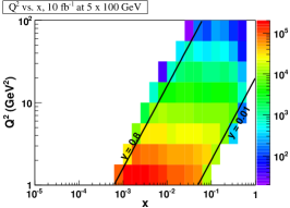
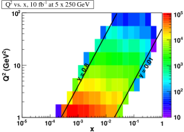
Figure 8: The distribution of statistics in each $\{{\cal Q}^{2},x_{\rm B}\}$ bin for eRHIC stage I (left and middle) and stage II (right) at a luminosity of $10\,{\rm fb}^{-1}$.

For the purpose of DVCS cross section measurements it is important to remove from the signal the background coming from the BH events. The latter is a QED process, well known to an uncertainty of the order of 3% coming from the uncertainty on the proton form factors. It can be subtracted from the signal by means of a MC technique. Thus, especially at a high luminosity machine like eRHIC where systematic uncertainties will dominate the measurements, it is important to minimize the BH contribution, particularly at low c.o.m. energy, where BH tends to dominate over the DVCS (see Sect. 2.1). The fraction of BH events has been estimated using a MC sample containing both DVCS and BH processes. The BH contamination was investigated for each $\{{\cal Q}^{2},x_{\rm B},t\}$ bin as a function of the electron energy loss $y$. After all BH suppression criteria have been applied it was found that at large c.o.m. energies the BH contamination grows from negligible (at low-$y$) to about 70% at $y\sim 0.6$ allowing for a safe BH subtraction, whereas for lower c.o.m. energies the BH contamination grows faster with $y$ and can be dominant depending on the bin; nevertheless most of the statistics at this low c.o.m. energy is contained in the safe region $y<0.3$.

Figure 8 compares the distribution of the statistics per bin for the eRHIC beam-energy configurations $5\times 100\operatorname{GeV}^{2}$, $5\times 250\operatorname{GeV}^{2}$ (both reachable at a stage I) and $20\times 250\operatorname{GeV}^{2}$ (available at a stage II), considering an integrated luminosity of $\sim 10\,{\rm fb}^{-1}$. The results shown in the present paper are based on simulated data samples corresponding to an integrated luminosity of $100\,{\rm fb}^{-1}$ for the $20\times 250\operatorname{GeV}^{2}$ configuration and $10\,{\rm fb}^{-1}$ for the $5\times 100\operatorname{GeV}^{2}$ configuration, both corresponding to approximately 1 year of data taking at eRHIC assuming a 50% operational efficiency. The data samples generated for the propose of measuring the differential cross section only contain the DVCS process whereas samples containing DVCS, BH, and their interference term have been generated for measurements of different single spin asymmetries.

All the generated events have been smeared according to expected momentum and angular resolutions. The statistical uncertainty for the differential cross section can be at small values of $-t$ as low as few percent; the same is true for the uncertainty for the extracted slope parameter $B$. This implies that the measurement is actually limited by systematics. For the purposes of the present work, a systematic uncertainty of 5% has been assumed, based on the experience at HERA and the expected coverage and technology improvements of the new detector at eRHIC. The overall systematic uncertainty, due to the uncertainty on the measurement of luminosity, is not considered for this paper as it simply affects the normalization of the cross section measurement.

4 Selected DVCS observables at EIC

As explained in Sect. 2, the isolation of CFFs is a rather intricate task, which can be only achieved by measuring a complete set of observables. However, we have also seen that photon helicity flip contributions, which are suppressed in DVCS kinematics, are not traceable in the present world data set. Hence, we restrict ourselves to four twist-two associated CFFs to study the physics case of DVCS measurements at a suggested eRHIC, giving emphasis to twist-two dominated observables. As motivated in Sect. 3, we choose two scenarios: one with a relatively low and another with a high c.o.m. energy, corresponding to the beam configurations

$$E_{e}\times E_{p}=5\times 100\operatorname{GeV}^{2}\quad\mbox{and}\quad E_{e}\times E_{p}=20\times 250\operatorname{GeV}^{2}.$$

For future DVCS measurements at $5\times 100\operatorname{GeV}^{2}$ it is maybe expected that the description of precise data in this region of transition to the small-$x_{\rm B}$ physics requires rather complex GPD models, which are not needed for the description of the present DVCS data. For the higher energy case it is expected that valence quark contributions are negligibly small and non-negligible CFFs

$$x_{\rm B}\times{\cal H}\quad\mbox{and potentially}\quad x_{\rm B}\times{\cal E}$$

are governed by an effective “pomeron” exchange in the $t$-channel, associated with both sea quarks and gluon contributions, and that they (moderately) grow with decreasing $x_{\rm B}$. Thereby, almost nothing is known about the CFF $\cal E$, which, as pointed out in Sect. 2.3, is not accessible from present DVCS measurements in neither the collider nor the fixed target mode. The available theoretical/phenomenological guidance is not yet fully trustworthy. On one hand a “pomeron” coupling to proton helicity non-conserved quantities such as the CFF $\cal E$ is phenomenologically not established, see Ref. Don05 and references therein. On the other hand a pomeron like behavior for the CFF $\cal E$ is perturbatively predicted by GPD evolution. A separate study on the access of GPD $E$ as well as the transverse spatial distribution of sea quarks and gluons at stage II will be presented in Sect. 5, which without additional information or assumptions is hard to achieve for EIC measurements at low beam energies.

We expect that the remaining two twist-two associated CFFs if multiplied with $x_{\rm B}$,

$$x_{\rm B}\times\widetilde{\cal H}\quad\mbox{and}\quad x_{\rm B}\times\overline{\cal E}\approx x_{\rm B}\times\frac{x_{\rm B}}{2-x_{\rm B}}\widetilde{\cal E},$$

go to zero in the small-$x_{\rm B}$ region. Note, however, that in contrast to the CFF ${\cal H}$, Regge phenomenology provides no clear guidance for their small-$x_{\rm B}$ behavior. The phenomenological situation is analogous to the polarized DIS function $g_{1}$ (GPD $\widetilde{H}$ embeds the polarized PDF $\Delta q$). We emphasize that these essentially unknown contributions may play a role at the stage I kinematics.

To cover possible scenarios, we employ in our studies three hybrid models, where sea quark and gluonic components of CFFs $\cal H$ and $\cal E$ are based on GPD models that include the perturbative evolution, while their valence quarks and remaining GPDs are treated with dispersion relations as described in Sect. 2.2 . Two of the models are pinned down from global fits to the world data of unpolarized DVCS measurements, which are described very well, despite having rather different partonic content. We now list the models and describe their main properties.

• KM10 describes the world data set of DVCS measurements using an unpolarized proton target. It contains the twist-two GPDs $H$ and $\widetilde{H}$, while the real part of helicity-flip CFFs $\cal E$ and $\widetilde{\cal E}$ are only given by subtraction constants in the dispersion relation (related to so-called $D$-term and pion pole contribution, respectively). Both GPD $\widetilde{H}$ and the (real) CFF $\widetilde{\cal E}$ are rather large and they are considered as effective degrees of freedom that allow to describe the unpolarized cross section measurements from the Hall A collaboration Munoz_Camacho:2006hx .

• KM10a is analogous to the KM10 model; however, the Hall A cross section measurements are not well described. In this model the GPD $H$ is the dominant one, $\widetilde{H}$ is set to zero, and $\widetilde{\cal E}$ contains only the pion pole, which is accounted in the standard way Mankiewicz:1998kg ; Frankfurt:1999xe .

• AFKM12 is a flexible GPD model for the small-$x$ region, specifically designed for the present study. It contains besides the sea quark and gluon GPDs $H^{\rm sea}$ and $H^{\rm G}$ also a flexible small-$x$ parametrization of GPDs $E^{\rm sea}$ and $E^{\rm G}$. All of these GPDs include a “pomeron” behavior, which can be individually adjusted at the input scale. The normalization of $E$-type GPDs is controlled by the anomalous magnetic moment of sea quarks $\kappa^{\rm sea}=1.5$, which is fixed to be positive and rather large. The parton polarized GPDs $\widetilde{H}$ and $\widetilde{E}$ are set to zero.

Our small-$x$ GPD models are set up in terms of (conformal) GPD moments rather than in $x$-space, at the input scale ${\cal Q}^{2}=4\operatorname{GeV}^{2}$ for four light quarks. They yield, similarly to other GPD models, the following effective functional form of CFFs:

$$\left\{{\cal H}\atop{\cal E}\right\}(x_{\rm B},t,{\cal Q}^{2})\sim\pi\left[i-\cot\left(\frac{\pi\alpha(t,{\cal Q}^{2})}{2}\right)\right]\xi^{-\alpha(t,{\cal Q}^{2})}\left\{h_{\alpha}\atop e_{\alpha}\right\}(t,{\cal Q}^{2})\,,$$ (35)

which resembles a Regge phenomenological ansatz with a linear “pomeron” trajectory

$$\alpha(t)=\alpha(t=0)+\alpha^{\prime}t.$$ (36)

In the KM10 and KM10a models a dipole parametrization $\left(1-\frac{t}{M^{2}}\right)^{-2}$ for the residual $t$-dependency was taken, while the AFKM12 model alternatively relies, as in the MILOU simulation, on an exponential ansatz $e^{bt}$. The boundary value of the residue $h_{\alpha}$ at $t=0$ depends on both the momentum fractions $N^{i}({\cal Q}^{2})$, carried by the unpolarized parton type $i$, and the skewness effect, parameterized in terms of two model parameters $s^{i}_{2}$ and $s^{i}_{4}$, which control both the normalization of the CFFs and their ${\cal Q}^{2}$ evolution; a detailed discussion is given in Kumericki:2007mh ; Kumericki:2009uq ; doi:10.1142/S201019451100167X . Analogously, we parameterize in the AFKM12 model the GPD $E$ with an independent set of parameters, however, here the momentum fractions $N^{i}({\cal Q}^{2})$ are replaced by the partonic gravitomagnetic moments ${\cal B}^{i}=N^{i}\kappa^{i}$, parameterized at the input scale by the product of the momentum fraction $N^{i}$ and the anomalous magnetic moments $\kappa^{i}$. The momentum and gravitomagnetic sum rules are utilized to fix the gluonic momentum fraction and gravitomagnetic moment, respectively. From a DIS fit the PDF-related parameters were found Kumericki:2009uq ,

$$N^{\rm sea}=0.152\,,\quad\alpha^{\rm sea}=\alpha_{E}^{\rm sea}=1.158\,,\quad\alpha^{\rm G}=\alpha_{E}^{\rm G}=1.247\,,$$ (37)

which we, for simplicity, also adopt for GPD $E$ in the AFKM12 model. Some other relevant model parameters are listed in Tab. 1, where, again for simplicity, we equate the Regge slope parameters of GPD $H$ and the residue slope parameter for GPD $E$ with those of GPD $H$,

$$\alpha^{\prime~{}{\rm G}}=\alpha^{\prime~{}{\rm sea}}\,\quad b^{\rm sea}_{E}=b^{\rm sea}\,,\quad b^{\rm G}_{E}=b^{\rm G}\,.$$ (38)

Finally, we specify the remaining GPDs on the cross-over line and the form of subtraction constants, where the CFFs are calculated from (29, 30, 31).

AmodelA	$\alpha^{\prime~{}{\rm sea}}$	$\kappa^{\rm sea}$	$\alpha_{E}^{\prime~{}{\rm sea}}$	$\alpha_{E}^{\prime~{}{\rm G}}$	$(M^{\rm sea})^{2}$	$(M^{\rm G})^{2}$	$b^{\rm sea}$	$b^{\rm G}$
KM10 ​​(a)	0.15	0.0	–	–	0.51(0.52)	0.7	–	–
AFKM12	0.10	1.5	0.02	0.05	–	–	2.8	2.0

end

AmodelA	$r$	$b$	$M$	$c$	$M_{c}$	$\widetilde{r}$	$\widetilde{b}$	$\widetilde{M}$	$r_{\pi}$	$M_{\pi}$
KM10 i	0.620	0.404	4.	8.777	0.975	7.759	2.050	0.884	3.536	4.020
KM10a	0.884	0.400	1.5	1.722	2.000	0.000	–	–	cf. PenPolGoe99	cf. PenPolGoe99

Table 1: Some selected model parameters for unpolarized sea quark and gluon GPDs (upper table), valence $H$ and $\widetilde{H}$ GPDs as well as for subtraction constants (lower table), where squared mass parameters are given in $\operatorname{GeV}^{2}$ and slope parameters $\alpha^{\prime}$ and $B$ in $\operatorname{GeV}^{-2}$.

Only the target helicity conserved GPDs on the cross-over line are modeled

$$H^{\rm val}(x,x,t) = \frac{1.35\,r}{1+x}\left(\frac{2x}{1+x}\right)^{-\alpha(t)}\left(\frac{1-x}{1+x}\right)^{b}\left(1-\frac{1-x}{1+x}\frac{t}{M^{\rm val}}\right)^{-1}\,,$$ (39)

$$\widetilde{H}(x,x,t) = \frac{0.6\,\widetilde{r}}{1+x}\left(\frac{2x}{1+x}\right)^{-\alpha(t)}\left(\frac{1-x}{1+x}\right)^{\widetilde{b}}\left(1-\frac{1-x}{1+x}\frac{t}{\widetilde{M}}\right)^{-1}\,.$$ (40)

Here, the skewness effect is parameterized by the ratios

$$r=\lim_{x\to 0}\frac{H(x,x,0)}{H(x,0,0)}\quad\mbox{and}\quad\widetilde{r}=\lim_{x\to 0}\frac{\widetilde{H}(x,x,0)}{\widetilde{H}(x,0,0)}\,,$$

$\alpha(t)=0.43+0.85\,t/{\rm GeV}^{2}$, $b$ ($\widetilde{b}$) controls the $x\to 1$ limit, $M^{\rm val}$ ( $\widetilde{M}$) the residual $t$-dependence, where $q(x)=H(x,0,0)$ ($\Delta q(x)=\widetilde{H}(x,0,0)$) are unpolarized (polarized) reference PDFs, e.g., the LO parametrization of Alekhin:2002fv (GehSti95 ). The subtraction constant is normalized by $c$ ($r_{\pi}$) and the cut-off mass $M_{c}$ ($M_{\pi}$) controls the $t$-dependence:

$${\cal C}(t)=\frac{c}{\left(1-\frac{t}{M_{c}^{2}}\right)^{2}}\,,\qquad\widetilde{\cal C}(t)=\frac{2.164\,r_{\pi}}{(m_{\pi}^{2}-t)\left(1-\frac{t}{M_{\pi}^{2}}\right)^{2}}\,,$$ (41)

where $m_{\pi}\approx 0.14\operatorname{GeV}$ is the pion mass and the normalization factor $2.164$ in the pion pole contribution matches the residue of the $t=m_{\pi}^{2}$ pole from the pseudo scalar form factor $2g_{A}M_{p}^{2}/(1+m_{\pi}^{2}/M_{\pi}^{2})$ with $M_{\pi}=1.17\operatorname{GeV}$. Note, however, that in the GPD framework the normalization of the pion pole contribution remains unknown. In the KM10a model we use the pion pole parametrization of PenPolGoe99 . More explanations on these simple parameterizations can be found in Kumericki:2009uq . The parameters of the KM10 and KM10a models are listed in Tab. 1.

In the remainder we illuminate the richness of a possible experimental DVCS program at an suggested EIC. Thereby, we will concentrate on observables that are dominated by twist-two associated CFFs. In Sect. 4.1 we restrict ourselves to the unpolarized cross section and in Sect. 4.2 to single spin asymmetry measurements. In Sect. 4.3 we will comment on further DVCS related measurements, which are interesting on their own, and we shortly discuss the use of an unpolarized positron beam to disentangle photon helicity non-flip contributions from longitudinal-transverse helicity ones.

4.1 Cross section measurements at stage I

As emphasized in Sect. 2.1, the separation of the measurable electroproduction cross section (2.1) into its three parts in the most model independent way and/or with a minimal set of assumptions is an important goal. So far the extraction of the $t$-differential DVCS cross section, entering in (2.1), has been only reached in the small-$x_{\rm B}$ and $0.1\operatorname{GeV}^{2}\leq-t\leq 0.8\operatorname{GeV}^{2}$ region by the H1 and ZEUS collaborations. Thereby, the subtraction method

$$\frac{d\sigma^{\mbox{\tiny DVCS}}(x_{\rm B},t,{\cal Q}^{2})}{dt}\simeq\frac{d\sigma^{\mbox{\tiny TOT}}(x_{\rm B},t,{\cal Q}^{2})}{dt}-\frac{d\sigma^{\mbox{\tiny BH}}(x_{\rm B},t,{\cal Q}^{2})}{dt},$$ (42)

was utilized, where the interference term could be safely neglected and the BH cross section was simulated. The latter was cross-checked experimentally in the BH dominated phase space region.

To understand whether such a subtraction procedure would be also reliable in the EIC kinematics and whether one can improve this method by utilizing the variable beam energy option, we consider first the generic dependence of the $t$-differential cross section (2.1) on its variables. According to what was explained in Sect. 2.1, for smaller value of $-t\gg-t_{\rm min}\approx x_{\rm B}^{2}M_{p}^{2}$ and large $y$ the BH cross section dominates, since it is enhanced by the kinematical prefactor $y^{2}/(-t{\cal Q}^{2})$. On the other hand in the limit $y\to 0$ both the BH cross section and the interference term drop out, where $\varepsilon(y=0)=1$ and, thus, the sum of the transverse and longitudinal DVCS cross sections can be accessed, see (21). Moreover, the interference term (12) has the same canonical $1/{\cal Q}^{4}$ scaling as the DVCS cross section (13), however, it has an additional prefactor $x_{\rm B}\,y$. Restricting ourselves to the dominant CFF ${\cal H}$, we find that the ratio of interference term (12, 14) to the sum of BH (17) and DVCS (18) cross sections is estimated, for smaller-$x_{\rm B}$ values, to be

$$\frac{d\sigma^{\mbox{\tiny\rm INT}}}{d\sigma^{\mbox{\tiny\rm BH}}+d\sigma^{\mbox{\tiny\rm DVCS}}}\sim 2x_{\rm B}\sqrt{\frac{-(1-y)t}{{\cal Q}^{2}}}\,\frac{F_{1}(t)\,\sqrt{\frac{-t(1-y)}{4y^{2}{\cal Q}^{2}}}\,\Re{\rm e}\,x_{\rm B}{\cal H}(x_{\rm B},t,{\cal Q}^{2})}{F_{1}^{2}(t)-\frac{t}{4M_{p}^{2}}F_{2}^{2}(t)+\frac{-t(1-y)}{4y^{2}{\cal Q}^{2}}\left|x_{\rm B}{\cal H}(x_{\rm B},t,{\cal Q}^{2})\right|^{2}}\,.$$ (43)

Obviously, the suppression factor $2x_{\rm B}\sqrt{-(1-y)t/{\cal Q}^{2}}\lesssim x_{\rm B}$ (DVCS requires $-t\ll{\cal Q}^{2}$ ) makes this ratio small for EIC kinematics. Moreover, we expect from Regge arguments, consistent with phenomenological findings, that the real part of the dominant CFF ${\cal H}$ is in the small- and even moderate-$x_{\rm B}$ region much smaller than its imaginary part (at least for smaller values of $-t$, see the results from HERMES in Fig. 3). We conclude that in most of the stage I bins, given in Sect. 3, the interference term is negligible and we can simplify the $t$-differential cross section (21) to

$$\frac{d\sigma^{\mbox{\tiny TOT}}}{dt}\approx\frac{y^{2}\left[\frac{d\sigma_{\rm T}^{\mbox{\tiny BH,red}}}{dt}+\varepsilon(y)\frac{d\sigma_{\rm L}^{\mbox{\tiny BH,red}}}{dt}\right]}{\left(1-y\frac{(1-x_{\rm B})t}{{\cal Q}^{2}+t}\right)\left(\frac{{\cal Q}^{2}+t}{{\cal Q}^{2}+x_{\rm B}t}-y\right)}+\frac{d\sigma^{\mbox{\tiny\rm DVCS}}(y)}{dt}$$ (44)

with $\frac{d\sigma^{DVCS}(y)}{dt}=\frac{d\sigma_{T}^{DVCS}}{dt}+\varepsilon(y)\frac{d\sigma_{L}^{DVCS}}{dt}.$ The smallness of the interference term has been also seen in numerical GPD model calculations. Thereby, the use of the approximate equations in Belitsky:2001ns naturally yields only incomplete cancelations in the $\phi$-integrated interference term. This causes the ratio (43) to appear proportional to $(-t/{\cal Q}^{2})^{3/2}$ rather than to $x_{\rm B}\times(-t/{\cal Q}^{2})^{1/2}$. Nevertheless, also in the MILOU simulations, based on the approximate equations in Belitsky:2001ns , the interference term turns out to be negligibly small.

For an EIC experiment the equation (44) provides a further handle to cross-check experimentally the BH subtraction procedure. However, we expect that a Rosenbluth separation of the transverse and longitudinal DVCS cross section will be difficult to achieve in the small $-t$ region. To suppress the BH contribution a relatively small $y$ is needed, which also means that the variation of $\varepsilon(y)$, which functional dependence can be mimicked by a truncated Taylor expansion $\varepsilon(y)\approx 1-\frac{y^{2}}{2}-\frac{y^{3}}{2},$ is only small. Moreover, if we stick to the twist-two expansion of the DVCS amplitude, the longitudinal DVCS cross section in the small-$x_{\rm B}$ region will be expressed by twist-three associated CFFs and this cross section will be kinematical suppressed by a factor $\widetilde{K}^{2}/{\cal Q}^{2}\approx-t/{\cal Q}^{2}$, see (13), (25) and (25). On the other hand these behaviors may offer the possibility of access to the twist-three contribution at larger values of $-t$, which, in turn, allows the variation of $y$ over a larger region. However, such an access may only be possible if the $t$-dependence of CFFs, as compared to that of electromagnetic form factors, is rather flat.

The transverse DVCS cross section contains both non-flip and transverse flip helicity amplitudes, where the latter would be perturbatively suppressed by $(\alpha_{s}/2\pi)^{2}$ or $1/{\cal Q}^{2}$ corrections. Neglecting the suppressed photon helicity flip contributions and switching to the GPD-inspired CFF basis (22), we can approximately write the DVCS cross section for stage I kinematics as

$$\frac{d\sigma^{\mbox{\tiny\rm DVCS}}}{dt}\approx\frac{\pi\alpha_{\rm em}^{2}}{{\cal Q}^{4}}\left[\frac{\big{|}x_{\rm B}{\cal H}\big{|}^{2}}{\left(1-\frac{x_{\rm B}}{2}\right)^{2}}-\frac{t\,\big{|}x_{\rm B}{\cal E}\big{|}^{2}}{4M^{2}_{p}}+\frac{\big{|}x_{\rm B}\widetilde{\cal H}\big{|}^{2}}{\left(1-\frac{x_{\rm B}}{2}\right)^{2}}-\frac{t\,\big{|}x_{\rm B}\overline{\cal E}\big{|}^{2}}{4M^{2}_{p}}-\frac{x_{\rm B}\,\Re{\rm e}\,\widetilde{\cal H}\,\overline{\cal E}^{\ast}}{1-\frac{x_{\rm B}}{2}}\right]\!\left(x_{\rm B},t,{\cal Q}^{2}\right),\\$$

where the functional form arises from the exact $\cal C$-coefficients by neglecting kinematically suppressed contributions of order ${\cal O}(x_{\rm B}^{2})$ and ${\cal O}(x_{\rm B}t/{\cal Q}^{2})$. As somehow expected, in our numerical studies it turned out that the DVCS cross section (4.1) for the $5\times 100\operatorname{GeV}^{2}$ beam configuration is rather sensitive to the choice of GPD model. To some extent this is also true for higher c.o.m. energies in the large $-t$ region. In other words, a definite conclusion whether the subtraction method in these kinematics will be possible, cannot be taken without actual data.

As mentioned in Sect. 3, the eRHIC option allows also at stage I to increase the proton beam energy, for kinematical coverage see Fig. 8. To illustrate the energy dependence of the DVCS cross section, we consider its ratio to the measurable electroproduction cross section

$$\frac{d\sigma^{\mbox{\tiny\rm DVCS}}}{d\sigma^{\mbox{\tiny\rm TOT}}}=\frac{\int_{-\pi}^{\pi}\!d\phi\,\frac{d\sigma^{ep\to ep\gamma,\mbox{\tiny\rm DVCS}}}{dx_{\rm B}dtd{\cal Q}^{2}d\phi}}{\int_{-\pi}^{\pi}\!d\phi\,\frac{d\sigma^{ep\to ep\gamma}}{dx_{\rm B}dtd{\cal Q}^{2}d\phi}}\,.$$ (45)

Considering again the CFF $\cal H$ as the dominant one and sticking to the small-$x_{\rm B}$ approximation with $-t\gg t_{\rm min}$ and $y<y_{\rm col}\approx 1$, we can estimate this ratio as

$$\frac{d\sigma^{\mbox{\tiny\rm DVCS}}}{d\sigma^{\mbox{\tiny\rm TOT}}}\sim\frac{\frac{-t(1-y)}{4y^{2}{\cal Q}^{2}}\left|x_{\rm B}{\cal H}(x_{\rm B},t,{\cal Q}^{2})\right|^{2}}{F_{1}^{2}(t)-\frac{t}{4M_{p}^{2}}F_{2}^{2}(t)+\frac{-t(1-y)}{4y^{2}{\cal Q}^{2}}\left|x_{\rm B}{\cal H}(x_{\rm B},t,{\cal Q}^{2})\right|^{2}}\,.$$ (46)

Clearly, as long as we stay away from $-t_{\rm min}$, which is at EIC not reachable in the considered bins, this ratio will get very small at low $-t$ and its behavior at large $-t<{\cal Q}^{2}$ depends on the $-t$ drop-off of CFFs.

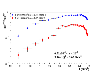
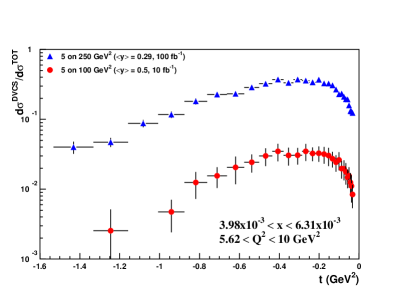
Figure 9: Cross section ratio (45) of the DVCS cross section to the photon electroproduction cross section (21) as function of $-t$ for two $x_{\rm B}-{\cal Q}^{2}$-bins and two different beam energy combinations.

In Fig. 9 we show the typical $t$-shape of this ratio for an exponential $t$-dependence at $5\times 100\operatorname{GeV}^{2}$ (circles) and $5\times 250\operatorname{GeV}^{2}$ (triangles) for two $\{x_{\rm B},{\cal Q}^{2}\}$-bins,

$$6.31\times 10^{-3}<x_{\rm B}<1.00\times 10^{-2} 3.16\operatorname{GeV}^{2}<{\cal Q}^{2}<5.62\operatorname{GeV}^{2}\mbox{ (left)}\,,$$ and

$$3.98\times 10^{-3}<x_{\rm B}<6.31\times 10^{-3} 5.62\operatorname{GeV}^{2}<{\cal Q}^{2}<10.0\operatorname{GeV}^{2}\mbox{ (right)}\,.$$ and

These results were simulated by MILOU, as described in Sect. 3. The statistical uncertainties are obtained including all the selection criteria to suppress the BH cross section also in the region where the DVCS cross section is extremely small. Clearly, the functional multi-variable dependencies, that are expected from the approximation (46), can be easily seen in the plots. In this specific GPD model, utilized in MILOU, the DVCS cross section is only accessible in a smaller set of $\{x_{\rm B},{\cal Q}^{2},t\}$-bins. However, as is clearly illustrated in Fig. 9, an increase of the proton beam energy from $100\operatorname{GeV}$ to $250\operatorname{GeV}$ allows to overcome such a potential limitation.

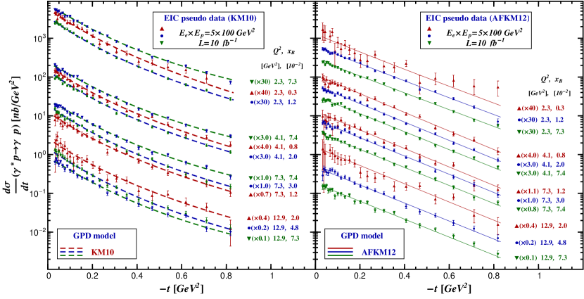
Figure 10: KM10 (left panel) and AFKM12 (right panel) model predictions of the differential DVCS cross section versus $-t$ for unpolarized beams with energies $E_{e}\times E_{p}=5\times 100\operatorname{GeV}^{2}$ and a luminosity of $10~{}{\rm fb}^{-1}$. The uncertainties of the EIC pseudo data contain statistical, 5% systematical, and uncertainties due to BH cross section subtraction, where for the latter a 3% uncertainty of the BH cross section has been assumed.

We take now the KM10 and AFKM12 predictions to illustrate that the DVCS cross section can be possibly obtained by a subtraction procedure (42) even at the low beam energy configuration $5\times 100\operatorname{GeV}^{2}$. Generally, these DVCS cross section predictions overshoot those of the MILOU simulations, on the other hand the KM10a model predictions are in agreement. Based on the MILOU simulations, described in Sect. 3, we obtain the statistical uncertainties for the model predictions by rescaling according to the ratios of the DVCS cross sections. All uncertainties (statistical, $5\%$ systematical, and subtraction uncertainty from a 3% error of the BH cross section) were added in quadrature and the predicted cross section for a kinematical point, given by the center of a three dimensional $\{x_{\rm B},{\cal Q}^{2},t\}$-bin, was assumed to be normally distributed.

In Fig. 10 we show the KM10 (left panel) and AFKM12 (right panel) model predictions for the DVCS cross section versus $-t$ for the $5\times 100\operatorname{GeV}^{2}$ beam energy configuration for four ${\cal Q}^{2}$ and three $x_{\rm B}$ bins. Apart from the different $t$-behavior, one notices model differences in the normalization at lower $-t$ values, in particular for the largest $x_{\rm B}$ values. One also realizes that in the KM10 model the cross section does not necessarily grow with decreasing $x_{\rm B}$ as it is the case for AFKM12 model (solid curves), containing only the sea quarks and gluon components of the CFFs $\cal H$ and $\cal E$. Both of these observations indicate that valence-like contributions to $\cal H$ and/or non-dominant CFFs can play a certain role at lower c.o.m. energies. In both panels the sizable uncertainties arise from the uncertainty of the BH cross section and, as expected, they appear for the low $x_{\rm B}$ bins, essentially, in the small $-t$ region and large $-t$ region. Note in Fig. 10 bins are not shown in which the DVCS cross section is entirely dominated by the subtraction uncertainties, i.e., we ignored bins with $y\gtrsim 0.25\cdots 0.4$. For values $-t>0.8\operatorname{GeV}^{2}$ (not shown) the uncertainties associated with the BH subtraction become also large, particularly for AFKM12 model which possesses an exponential $t$-dependence. We remind that all models, including MILOU, describe the H1/ZEUS DVCS cross sections measurements very well (see left panel of Fig. 13) for which the aforementioned contributions play a minor role.

Let us summarize the lessons for an unpolarized DVCS cross section measurement at rather low EIC energies. Certainly, it is safe to expect that the electroproduction cross sections, i.e., containing all three terms, are large enough to provide precise data, at present not available in this kinematical region of transition to small $x_{\rm B}$. Such data can be immediately included in global GPD fits; however, model assumptions will affect the partonic interpretation of such measurements. The isolation of the DVCS cross section is probably only feasible in a limited phase space (lower $y$ values, limited $-t$ values). Even in the case that this problem can be overcome by a (partial) Rosenbluth separation, the measurements would only provide a very qualitative insight in the transverse distribution of partons, since the separation of different CFF contributions is based on assumptions. Hence, a measurement of further observables is needed, which allows for a separation of the various CFFs contributions.

4.2 Single spin asymmetry measurements

Measuring the differences of spin-dependent cross sections (32) for unpolarized, longitudinally and transversely polarized protons allows the access of the imaginary part of CFFs in a much cleaner manner than utilizing asymmetries. In such measurements one may use harmonic analysis to access the imaginary parts of twist-two associated CFFs from the first odd harmonics, occurring from the interference of the BH and DVCS amplitudes. However, even these observables are contaminated by power-suppressed helicity flip contributions that stem from both the interference and DVCS squared term. The latter contamination can be eliminated if lepton beams of both charges are available, see discussion in the next section. This allows then for a harmonic analysis, aiming to isolate the imaginary parts of twist-two associated CFFs from the remaining ones. In this way one can separate to some extent twist-two, twist-three, and gluon transversity contributions. What is the best strategy to analyze a high quality data set, measured in an experiment where only an electron beam is available, is not so obvious at present. One may hope that, as in the case of unpolarized electroproduction cross section, considered in Sect. 2.1, a common Fourier analysis will finally yield some simplifications and may even allow to employ the Rosenbluth separation method to some extent.

For purpose of illustration we focus in the following on twist-two GPD model predictions for single spin asymmetries rather than on spin-dependent cross section differences (32). In Fig. 11 we show pseudo data that are generated using the KM10 model, and randomized according to the uncertainties as specified in Sect. 3 (rescaled statistical errors from MILOU simulations, $5\%$ systematical uncertainty on cross section level, $5\%$ normalization uncertainty for the polarization measurement). The error propagation from the $\phi$-dependent cross section to harmonic amplitudes was simply done by fitting. Note that the uncertainty for the projection asymptotically scales for the $N$ $\phi$-bins as $1/\sqrt{N}$, except for the zeroth harmonic for which scaling is $1/\sqrt{2N}$. We note that the polarization error should be treated as an overall normalization uncertainty, which, however, was not done here. Hence, the projections on the first harmonic in Fig. 11 have an additional normalization uncertainty, essentially given by the polarization uncertainty.

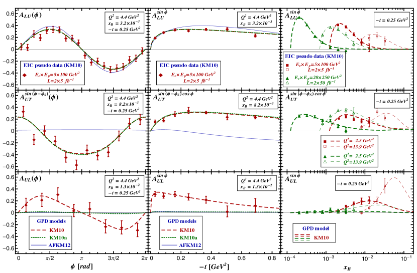
Figure 11: KM10 model predictions for DVCS single spin asymmetries: electron (47) [upper], transverse proton (48) [middle] and longitudinal proton (50) [lower] with $E_{e}\times E_{p}=5\times 100\operatorname{GeV}^{2}$ (diamonds,squares) and $E_{e}\times E_{p}=20\times 250\operatorname{GeV}^{2}$ (triangles) EIC settings. Asymmetries versus azimuthal angle $\phi$ for one selected bin ($x_{\rm B}=8.2\times 10^{-3},-t=0.25\operatorname{GeV}^{2},{\cal Q}^{2}=4.4\operatorname{GeV}^{2}$) at $5\times 100\operatorname{GeV}^{2}$ are shown in the left column for various GPD models: KM10 (dashed), KM10a (dotted), and AFKM12 (solid). In the middle column the $t$-dependence for the projection on the first non-vanishing harmonic is displayed for the same $x_{\rm B}$, ${\cal Q}^{2}$ and beam energy values. In the right column the $x_{\rm B}$-dependencies is shown for the KM10 model prediction at $-t=0.25\operatorname{GeV}^{2}$, two different ${\cal Q}^{2}$ values, ${\cal Q}^{2}=2.5\operatorname{GeV}^{2}$ (filled squares and triangles, thick curves) and ${\cal Q}^{2}=13.9\operatorname{GeV}^{2}$ (empty squares and triangles, thin curves), and two different choices of beam energies, $5\times 100\operatorname{GeV}^{2}$ (red) and $20\times 250\operatorname{GeV}^{2}$ (green).

The upper panels in Fig. 11 show for a proton beam the electron beam spin asymmetry (33) as function of the azimuthal angle $\phi$ for one selected bin with $5\times 100\operatorname{GeV}^{2}$ beam energies (left panel), its projection on the dominant first $\sin\phi$ harmonic,

$$A_{\rm LU}^{\sin\phi}\propto\frac{y\sqrt{1-y}}{2-2y+y^{2}}\sqrt{\frac{-t}{y^{2}{\cal Q}^{2}}}\times x_{\rm B}\,\Im{\rm m}\left[F_{1}{\cal H}-\frac{t}{4M_{p}^{2}}F_{2}{\cal E}+\frac{x_{\rm B}}{2}(F_{1}+F_{2})\widetilde{\cal H}\right](x_{\rm B},t,{\cal Q}^{2})+\cdots,$$ (47)

as function of $-t$ (middle panel), and versus $x_{\rm B}$ for a low ${\cal Q}^{2}=2.5\operatorname{GeV}^{2}$ and a high ${\cal Q}^{2}=13.9\operatorname{GeV}^{2}$ value (right panel). The asymmetry is dominated by helicity conserved CFF ${\cal H}$ and proportional to the electron energy loss $y$. Consequently, if $y$ is not too small, the asymmetry might be rather sizable over a large kinematical region, shown for $5\times 100\operatorname{GeV}^{2}$ (squares, thick curves) and $20\times 250\operatorname{GeV}^{2}$ (triangles, thin curves). The CFF $\cal E$ appears with a kinematic suppression factor $t/4M_{p}^{2}$, induced by a proton helicity flip, and remaining CFFs also contribute, which is in (47) indicated by the ellipsis that include also further kinematically suppressed contributions. Comparing the different predictions of the KM10 (dashed), KM10a (dotted), and AFKM12 (solid) models, one realizes that the contaminations of this asymmetry by other CFFs are in fact small. Our $\cal E$ enhanced model prediction only slightly differs from the other ones at $t\sim 0.5\,\operatorname{GeV}^{2}$. It is noted that for a neutron target the ${\cal H}$ contribution is suppressed by the accompanying Dirac form factor $F^{n}_{1}$ ($F_{1}^{n}(t=0)=0$), making this asymmetry sensitive to the CFF ${\cal E}$. However, in this case one expects a smaller single beam spin asymmetry that is also contaminated by other non-dominant CFF contributions.

A single spin asymmetry measurement with a transversely polarized proton beam, cf. (33), provides another handle on the imaginary part of the helicity-flip CFF ${\cal E}$. This asymmetry has in addition to the $\phi$ dependence a $\phi-\phi_{S}$ modulation. If the target spin in such a frame is perpendicular to the reaction plane (e.g., $\phi-\phi_{S}=\pi/2$), the asymmetry

$$A^{\sin(\phi-\phi_{S})\cos\phi}_{\rm UT}\propto\frac{\sqrt{1-y}}{2-y}\frac{-t}{2y\,M_{p}{\cal Q}}\times x_{\rm B}\Im{\rm m}\left[F_{2}{\cal H}-F_{1}{\cal E}+\frac{x_{\rm B}}{2}(F_{1}+F_{2})\overline{\cal E}\right](x_{\rm B},t,{\cal Q}^{2})+\cdots$$ (48)

is dominated by a linear combination of ${\cal H}$ and ${\cal E}$ CFFs. In the case that the target spin is aligned with the reaction plane (e.g., $\phi-\phi_{S}=0$) the asymmetry

$$A^{\cos(\phi-\phi_{S})\sin\phi}_{\rm UT}\propto\frac{\sqrt{1-y}}{2-y}\frac{-t}{2y\,M_{p}{\cal Q}}\times x_{\rm B}\Im{\rm m}\left[F_{2}\widetilde{\cal H}-F_{1}\overline{\cal E}\right](x_{\rm B},t,{\cal Q}^{2})+\cdots$$ (49)

is formally dominated by a linear combination of CFFs $\widetilde{\cal H}$ and $\overline{\cal E}$, cf. (20). In these asymmetries an additional relative kinematical factor $\sqrt{-t/4M_{p}^{2}}$ appears. The middle row in Fig. 11 shows the $\sin(\phi-\phi_{S})$ projection of the transverse proton beam spin asymmetry, which can also be rather large over a wide kinematical range. As in the case of the unpolarized cross section, discussed in the preceding section, this is caused by the fact that at smaller values of $x_{\rm B}$ the “pomeron” behavior in ${\cal H}$ overtakes the kinematical suppression factors, see dashed and dotted curves. We may assume that such a “pomeron” behavior is also contained in ${\cal E}$. For our choice of $\kappa^{\rm sea}=1.5$ the $\cal E$ contribution will mostly cancel the ${\cal H}$ contribution, see (48) where $F_{2}(t=0)\approx 1.79$. In contrast to the electron beam spin asymmetry, for a neutron target the asymmetry is now more sensitive to the helicity conserving CFF $\cal H$. For the $\cos(\phi-\phi_{S})$ projection of the transverse proton beam spin asymmetry (49) the common expectation is that the parity-odd CFFs $\widetilde{\cal H}$ and $\overline{\cal E}$ behave more gently at small $x_{\rm B}$ and, hence, we expect that this observable is small in the EIC kinematics (not shown).

Finally, we consider the longitudinally polarized proton beam spin asymmetry. Its projection on the dominant ${\sin\phi}$ harmonic reads

$$A^{\sin\phi}_{\rm UL}\propto\frac{\sqrt{1-y}}{2-y}\sqrt{\frac{-t}{y^{2}{\cal Q}^{2}}}\times x_{\rm B}\Im{\rm m}\left[F_{1}\widetilde{\cal H}-\left(\!\frac{x_{\rm B}}{2}F_{1}+\frac{t}{4M_{p}^{2}}F_{2}\!\right)\overline{\cal E}+\frac{x_{\rm B}}{2}(F_{1}+F_{2}){\cal H}\right]+\cdots.$$ (50)

It is sensitive to the imaginary part of CFF $\widetilde{\cal H}$ and $\overline{\cal E}$, and other CFFs might contribute as well. As already noted, one expects that here the dominant CFF $\widetilde{\cal H}$ behaves gently at small $x_{\rm B}$ and models that incorporate such a behavior predict a rather tiny asymmetry (dotted and solid lines). In contrast, in the KM10 model (dashed line), a rather big GPD $\widetilde{H}$ has been incorporated with a generic $1/\sqrt{x_{\rm B}}$ behavior at small $x_{\rm B}$. Hence, we get a sizable asymmetry for $5\times 100\operatorname{GeV}^{2}$ beam energies which is getting smaller at higher beam energies $20\times 250\operatorname{GeV}^{2}$, see lower row on Fig. 11. We emphasize again that not much is known about the small-$x_{\rm B}$ behavior of CFF $\widetilde{\cal H}$. We add that for a neutron target the asymmetry becomes sensitive to the CFF $\overline{\cal E}$.

Let us summarize the lessons from the approximated equations (47–50), quantified by numerics. The experimentally established ‘pomeron’ behavior of the CFF $\cal H$ predicts a large single beam spin and a large $\cos(\phi-\phi_{S})$ projection of the transverse proton beam spin asymmetry for the EIC kinematics. If $\cal E$ contains also a ‘pomeron’ behavior, the latter asymmetry can be weakened (amplified) for a positive (negative) imaginary part of $\cal E$. The remaining two single spin asymmetries cannot be predicted easily; however, based on common phenomenological/theoretical wisdom they are probably small. Let us note that the normalization of these asymmetries obviously depends also on the real part of the twist-two associated CFFs and the remaining eight ones. As advocated above, a measurement of cross section differences are not affected by this normalization uncertainty.

4.3 Further EIC opportunities

An EIC machine provides further opportunities for DVCS studies:

• Double spin flip experiments provide a handle on the real part of CFFs, however, in such measurements the spin-dependent BH cross section contributes.

• As demonstrated by the HERMES collaboration, having a positron beam at hand allows also to separate the interference and DVCS harmonics in single spin target experiments. Measuring spin-dependent cross sections in the charge odd sector (interference term) and the charge even sector allows to extract CFFs from experimental measurements, based on minimal assumptions.

• The large kinematical coverage of the proposed high-luminosity EIC (see Fig. 5) and the partial overlap with JLAB 12GeV kinematics raises the question: Can one utilize evolution, even at moderate $x_{\rm B}$ values, to access GPDs away from their cross-over line?

• Photon electroproduction off the neutron offers the possibility for a flavor separation.

• Photon electroproduction off nuclei is a mostly unexplored experimental field.

Below we will discuss a minimalistic version of the second point in more detail, namely, having an unpolarized positron beam at hand. Let us mention here that a study of GPD evolution was presented in Ref. Kumericki:2011zc , however, we may conclude here that a wide coverage in ${\cal Q}^{2}$ is extremely helpful in getting constraints on GPDs away from the cross-over line, however, a “measurement” of the GPD in the outer region certainly cannot be reached. DVCS on a “neutron target” is certainly needed for a GPD flavor decomposition. However, this program is more complicated than in DIS, since in the interference term the various CFFs are accompanied by nucleon form factors, see short discussions in the previous section. We will not discuss DVCS off nuclei, which is interesting in itself. It has been worked out theoretically for a spin-zero target, where one can adopt the equation from Belitsky:2000vk , and to some extent also for spin-one target Berger:2001zb ; Kirchner:2003wt ; Cano:2003ju , while the formalism for spin-1/2 nuclei can be adopted from the proton.

We should also emphasize the EIC opportunities for Compton scattering measurements below the deeply virtual regime.

• Quasi-real Compton scattering can be measured over a rather wide energy range in anti-tagged electron scattering experiments, where the VCS cross section is peaked at ${\cal Q}^{2}\sim 0$.

• We expect that at stage I binning of low photon virtualities, i.e., ${\cal Q}^{2}<1\operatorname{GeV}^{2}$, will be possible.

Such measurements will provide understanding on the transition from the deeply virtual to the quasi-real regime. This, in turn, is needed if radiative electromagnetic corrections to photon electroproduction are to be elaborated in a more complete manner than they presently are.

Finally, we should remind that other exclusive channels can be measured at EIC:

• Deeply virtual production of light vector mesons can be employed for a partial flavor separation of quark GPDs.

• $J/\Psi$ production gives naturally access to the gluon GPD.

• Also, experimental studies on deeply virtual production of pseudo scalar mesons, the production of two final meson states, time-like DVCS, and double DVCS may turn out to be feasible.

We would like to add that deeply virtual production of light vector mesons and DVCS measurements at HERA collider experiments can be simultaneously described with a GPD formalisms Meskauskas:2011aa ; Kroll:2012sm . Whether the measurements, listed in the last item above, are actually feasible at EIC, can only be stated in terms of models. Thereby, based on phenomenological knowledge of the dominant GPD $H$, cross sections for time-like Berger:2001xd ; Moutarde:2013qs and/or double Guidal:2002kt ; Belitsky:2002tf ; Belitsky:2003fj DVCS might be more or less realistically estimated, however, were not part of our studies.

4.3.1 Uses of an unpolarized positron beam

The isolation of the interference term, which contains the most valuable information on CFFs, is most easily done by forming charge asymmetries, which require a positron beam. We emphasize again, that the alternative Rosenbluth separation is expected to be more intricate and has not been so far either considered theoretically or explored experimentally (e.g., by the use of approximated expressions). Forming differences and sums of spin-dependent cross section measurements with both kinds of lepton beams allows to extract the pure interference and DVCS squared terms and might allow to quantify twist-three and gluon transversity effects. From such experiments one can extract the imaginary part of CFFs. Note that only an unpolarized positron beam is needed to perform such a program for the single proton spin asymmetries – of course, for the projection of the single electron spin asymmetry a polarized positron beam would be needed. In double spin flip measurements one can use the same procedure to access the real part of the CFFs. Although existing data indicate that twist-three effects are small, as it is expected based on kinematic factors, the twist-three related CFFs are not necessarily small. Surely, one needs very high precision data to extract non-dominant twist-two CFFs or twist-three related ones. However, even obtaining only an upper limit is important for a determination of the systematic uncertainties of the (dominant) twist-two CFFs.

Let us consider here only the lepton beam charge asymmetry (34) for an unpolarized proton. Its first harmonic is dominated by the real part of the twist-two related CFFs $\cal H$ and $\cal E$, rather analogous to equation (47) for the electron beam spin asymmetry,

$$A_{\rm C}^{\cos\phi}\propto\frac{\sqrt{1-y}}{2-y}\sqrt{\frac{-t}{y^{2}{\cal Q}^{2}}}\times x_{\rm B}\,\Re{\rm e}\left[F_{1}{\cal H}-\frac{t}{4M_{p}^{2}}F_{2}{\cal E}+\frac{x_{\rm B}}{2}(F_{1}+F_{2})\widetilde{\cal H}\right](x_{\rm B},t,{\cal Q}^{2})+\cdots\,.$$ (51)

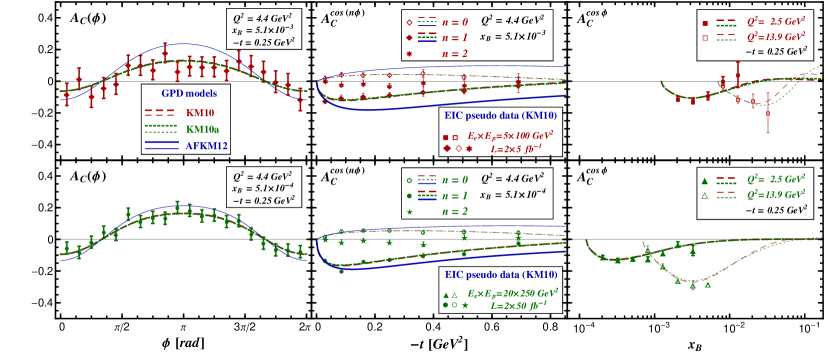
Figure 12: KM10 (dashed), KM10a (dotted), and AFKM12 (solid) model predictions for the DVCS lepton beam charge asymmetry (34, 51) with $E_{e}\times E_{p}=5\times 100\operatorname{GeV}^{2}$ (upper row) and $E_{e}\times E_{p}=20\times 250\operatorname{GeV}^{2}$ (lower row). Left column: $A_{\rm C}$ versus $\phi$ for $x_{\rm B}=5.1\times 10^{-3}$, ${\cal Q}^{2}=4.4~{}{\rm GeV}^{2}$, and $t=-0.25~{}{\rm GeV}^{2}$ (upper panel) and $x_{\rm B}=5.1\times 10^{-4}$, ${\cal Q}^{2}=4.4~{}{\rm GeV}^{2}$, and $t=-0.25~{}{\rm GeV}^{2}$ (lower panel). Middle column: $A_{\rm C}^{\cos(n\phi)}$ amplitudes versus $-t$ at same $x_{\rm B}$ and ${\cal Q}^{2}$ values for $n=1$ (filled diamonds and circles, thick curves), $n=0$ (empty diamonds and circles, thin curves), and $n=2$ (stars). Right column: Dominant amplitude $A_{\rm C}^{\cos(\phi)}$ versus $x_{\rm B}$ for ${\cal Q}^{2}=2.5\operatorname{GeV}^{2}$ (thick curves) and ${\cal Q}^{2}=13.9\operatorname{GeV}^{2}$ (thin curves) at $t=-0.25\operatorname{GeV}^{2}$.

It is shown in Fig. 12 that the GPD models predict a rather sizable lepton beam charge asymmetries for both $5\times 100\operatorname{GeV}^{2}$ (upper row) and $20\times 250\operatorname{GeV}^{2}$ (lower row) beam energies. As for the electron beam spin asymmetry (upper row on Fig. 11), the predictions from the KM10 (dashed curves) and KM10a (dotted curves) models are almost the same, illustrating that the CFF $\widetilde{\cal H}$ contribution is rather unimportant in this observable ($\widetilde{\cal E}$ drops exactly out here), while the small deviation of AFKM12 model (solid line) indicate some sensitivity to CFF $\cal E$. The sign of this asymmetry is governed by the effective ‘pomeron’ trajectory $\alpha^{\mathbb{P}}\gtrsim 1$. It has in the transition from the valence to the sea quark region a node (see upper right panel) with its position depending on $-t$. In the middle column we show besides the projection on the first even harmonic (filled diamonds and triangles) also the projection on the zeroth harmonic (empty diamonds and triangles), which is dominated by twist-two associated CFFs and, thus, (anti)correlated with the first harmonic. The second harmonic (stars) is sensitive to twist-three associated CFFs, which are set here to zero, and also depend on the twist-two associated CFFs. Therefore, the latter induce only a small deviation, compatible with zero within one standard deviation.

5 Partonic interpretation at small $x_{\rm B}$

Intensive GPD studies (up to NNLO accuracy) of small-$x_{\rm B}$ DVCS data measured by H1 and ZEUS collaborations have been performed, where it turned out that the functional form of the $t$-dependence cannot be pinned down and an access to the CFF $\cal E$ is not feasible when having only unpolarized DVCS cross section and the lepton beam charge asymmetry measurements Aaron:2009ac available Kumericki:2009uq . A high-luminosity EIC experiment with transversely polarized protons certainly provides the opportunity for precise measurements of CFFs and to explore their partonic interpretation in the small-$x_{\rm B}$ region, i.e., $x_{\rm B}<0.01$. As we argued in Sect. 4, the set of relevant twist-two associated CFFs is then reduced to $\cal H$ and $\cal E$ only, and, moreover, valence quark contributions can be safely neglected. From our discussion there it is also obvious that the former assumption, which is used now, can be experimentally cross-checked. We will also use the fact that the real parts of the remaining two CFFs is locally tied to their imaginary parts, see (35), which is implemented in our GPD model and is in fact a more general consequence of the dispersion relation and the effective ‘pomeron’ behavior. Hence, we can restrict ourselves to two observables, namely, the unpolarized DVCS cross section (4.1) and the single transverse proton beam asymmetry (48), which now simplify to

$$\frac{d\sigma^{\rm DVCS}}{dt}(x_{\rm B},t,{\cal Q}^{2}) \approx \frac{\pi\alpha^{2}x_{\rm B}^{2}}{{\cal Q}^{4}}\left[\left|{\cal H}\right|^{2}-\frac{t}{4M^{2}_{p}}\left|{\cal E}\right|^{2}\right]\left(x_{\rm B},t,{\cal Q}^{2}\right)\,,$$ (52)

$$A^{\sin(\phi-\phi_{S})\cos\phi}_{\rm UT} \propto \frac{\sqrt{1-y}}{2-y}\frac{-t}{2y\,M_{p}{\cal Q}}\times x_{\rm B}\Im{\rm m}\left[F_{2}{\cal H}-F_{1}{\cal E}\right](x_{\rm B},t,{\cal Q}^{2}).$$ (53)

In the partonic interpretation of DVCS data we are in the first place interested in the transverse distribution of sea quarks and gluons at small $x_{\rm B}$ for an unpolarized and for a transversely polarized proton. In Sec. 5.1 we explore by least-squares fitting the extraction of both GPD $H$ and $E$ from the aforementioned observables at stage II of an EIC. In Sect. 5.2 we present a detailed study of the extraction of transverse polarized parton distributions. We also perform there the Fourier transform of our GPD model fit results to the impact space, where experimental uncertainties are propagated and extrapolation errors are taken into account. Finally, in Sect. 5.3 we discuss the importance of such a measurement for the qualitative understanding of the proton spin decomposition.

5.1 Extraction of GPDs $H$ and $E$ from high energy EIC pseudo data

To illuminate how GPDs are experimentally constrained in the small-$x$ region at present, we will present here also new fits to the world DVCS data set at large $W$ (small $x_{\rm B}$) that includes the propagation of experimental uncertainties.

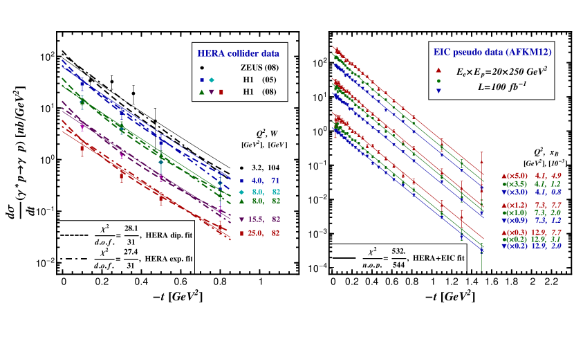
Figure 13: A model dependent extraction of GPD $H$ from cross section measurements of the H1/ZEUS collaborations (left) and from a combined fit that includes EIC pseudo data (right) with beam energies $E_{e}\times E_{p}=20\times 250\operatorname{GeV}^{2}$. The HERA collider data are taken from Chekanov:2008vy (circle), Aktas:2005ty (squares,diamonds), and Aaron:2009ac (triangle-up, triangle-down, rectangle).

At the HERA collider experiments H1 Adloff:2001cn ; Aktas:2005ty ; Aaron:2007ab ; Aaron:2009ac and ZEUS Chekanov:2003ya ; Chekanov:2008vy the unpolarized DVCS cross section could be measured at large $W$, $-t<1\,\operatorname{GeV}^{2}$, and with a large lever arm in ${\cal Q}^{2}$. Although $\sim 200$ data points were published, we only consider 35 as statistically independent. Apart from those for the differential cross section that are displayed on the left panel on Fig. 13 versus $-t$ we also included the following $t$-integrated cross section measurements from ZEUS

$$7.5\operatorname{GeV}^{2}\leq\left<{\cal Q}^{2}\right>\leq 85\operatorname{GeV}^{2} \left<W\right>=\phantom{0}89\operatorname{GeV}\;\mbox{\cite[cite]{\@@bibref{Authors Phrase1YearPhrase2}{Chekanov:2003ya}{\@@citephrase{(}}{\@@citephrase{)}}}},$$ (54)

$$7.5\operatorname{GeV}^{2}\leq\left<{\cal Q}^{2}\right>\leq 70\operatorname{GeV}^{2} \left<W\right>=104\operatorname{GeV}\;\mbox{\cite[cite]{\@@bibref{Authors Phrase1YearPhrase2}{Chekanov:2008vy}{\@@citephrase{(}}{\@@citephrase{)}}}}.$$

In our LO fits to these data we can only ask for the sea quark and gluonic components of GPD $H$, where both components can be separated to some extent due to the large ${\cal Q}^{2}$ lever arm Kumericki:2009uq . Since the experimental uncertainties are large, the functional form of the $-t$ dependence for sea quark (and gluon) GPD $H$ cannot be determined by $\chi^{2}/{\rm d.o.f.}\approx 1$ model fits, done here at LO with a dipole (dashed) or an exponential (dash-dotted) residual $t$-dependence. Thereby, also the “pomeron” slope parameter $\alpha^{\prime}$ for the sea quark (and gluon) content cannot be determined.

$H$	$N$	$\alpha$	$\alpha^{\prime}\;[\operatorname{GeV}^{-2}]$	$b\;[\operatorname{GeV}^{-2}]$	$s_{2}$	$s_{4}$
$p_{0}^{\rm sea}$	0.152	1.158	0.100	2.800	$\phantom{-}0.513$	$-0.210$
$p^{\rm sea}$	-	-	0.090	2.858	$\phantom{-}0.508$	$-0.208$
$\delta p^{\rm sea}$	-	-	0.009	0.035	$\phantom{-}0.038$	$\phantom{-}0.011$
$p_{0}^{\rm G}$	(0.448)	1.247	0.100	2.000	$-4.806$	$\phantom{-}1.864$
$p^{\rm G}$	-	-	0.063	2.086	$-4.739$	$\phantom{-}1.835$
$\delta p^{\rm G}$	-	-	0.088	0.163	$\phantom{-}0.212$	$\phantom{-}0.106$
$E$	$\kappa$	$\alpha$	$\alpha^{\prime}\;[\operatorname{GeV}^{-2}]$	$b\;[\operatorname{GeV}^{-2}]$	$s_{2}$	$s_{4}$
$p_{0}^{\rm sea}$	1.500	1.158	0.020	2.800	$\phantom{-}0.513$	$-0.210$
$p^{\rm sea}$	1.451	1.164	0.023	2.779	$\phantom{-}0.524$	$-0.213$
$\delta p^{\rm sea}$	0.307	0.005	0.012	0.049	$\phantom{-}0.104$	$\phantom{-}0.026$
$p_{0}^{\rm G}$	$(-0.51)$	1.247	0.050	2.000	$-4.806$	$\phantom{-}1.864$
$p^{\rm G}$	$(-0.49)$	1.295	0.001	1.961	$-4.687$	$\phantom{-}1.803$
$\delta p^{\rm G}$	$(0.06)$	0.216	0.252	1.092	$\phantom{-}0.048$	$\phantom{-}0.077$

Table 2: AFKM12 model parameters ($p_{0}$) and their fitted values ($p$) together with standard uncertainties ($\delta p$) for sea quarks (superscript ^sea) and gluon (superscript ^G) components of GPDs $H$ and $E$ at the input scale ${\cal Q}^{2}_{0}=4\operatorname{GeV}^{2}$. The values in parentheses are fixed by sum rules.

To explore the potential of the EIC measurements at stage II, we use in the following pseudo data for the unpolarized DVCS cross section (52) and the transverse target spin asymmetry (53) for the beam energies $20\times 250\operatorname{GeV}^{2}$, as specified in Sect. 3. Thereby, we utilized the flexible AFKM12 model, introduced in Sect. 4, in which GPD $H$ and $E$ have a different “pomeron” slope parameters, see $p_{0}$ values in Tab. 2, but the same residual $t$-dependencies. This choice guarantees that positivity conditions for GPDs at zero skewness are mostly satisfied EIC11Die . The experimental uncertainties were estimated as before (statistical uncertainties from the MILOU simulation, which are rescaled for the DVCS cross section, $5\%$ systematic uncertainty on cross section level, $3\%$ uncertainty of the BH cross section in the subtraction procedure (42), and $5\%$ beam polarization uncertainty). The exponential $t$-dependence of the CFFs drastically increases the subtraction uncertainty at large $-t$, and the net uncertainty in this region can become very large at larger $y$ values (lower $x_{\rm B}$ values in particular at low ${\cal Q}^{2}$), see right panel on Fig. 13. Since for the GPD $E$ we took a model with a positive $\kappa^{\rm sea}=1.5$, the transverse target asymmetry is becoming small. Fig. 14 shows the pseudo data for this asymmetry together with the model curve (solid), used to generate the asymmetry. Also shown is the prediction from an analogous model which, however, has a negative $\kappa^{\rm sea}=-1.5$ value (dashed curves) and one with vanishing CFF $\cal E$ (dash-dotted curves). Certainly, the predictions of all these three models are experimentally distinguishable.

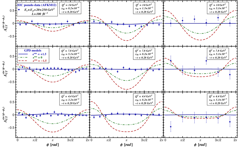
Figure 14: EIC pseudo data (diamonds) for the transverse target spin asymmetry (53) at beam energies $E_{e}\times E_{p}=20\times 250\operatorname{GeV}^{2}$ are shown together with AFKM12 GPD model predictions, where GPD $E^{\rm sea}$ is taken as large positive (solid), vanishing (dot-dashed), and large negative (dashed), respectively.

We performed a combined least-squares fit to the EIC pseudo data for the unpolarized DVCS cross section and the single transverse proton beam asymmetry together with the HERA collider measurements, shown in Fig. 13 and (54). Altogether we included $2732$ data points, where the EIC pseudo data were generated as specified above and contain 509 data points for the unpolarized cross section, obtained from 21 $\{{\cal Q}^{2},x_{\rm B}\}$-bins:

$$\phantom{0}3.16\operatorname{GeV}^{2}\leq{\cal Q}^{2}<\phantom{0}5.62\operatorname{GeV}^{2}\,, 2.5\times 10^{-4}\leq x_{\rm B}\leq 1.0\times 10^{-2}\;(8\;\mbox{bins}),$$

$$\phantom{0}5.62\operatorname{GeV}^{2}\leq{\cal Q}^{2}<10.00\operatorname{GeV}^{2}\,, 4.0\times 10^{-4}\leq x_{\rm B}\leq 1.0\times 10^{-2}\;(7\;\mbox{bins}),$$ (55)

$$10.00\operatorname{GeV}^{2}\leq{\cal Q}^{2}\leq 17.78\operatorname{GeV}^{2}\,, 6.3\times 10^{-4}\leq x_{\rm B}\leq 1.0\times 10^{-2}\;(6\;\mbox{bins}),$$

and 2188 data points for the single transverse beam spin asymmetry as function of $\phi$, obtained from 24 $\{{\cal Q}^{2},x_{\rm B}\}$-bins:

$$\phantom{0}3.16\operatorname{GeV}^{2}\leq{\cal Q}^{2}<\phantom{0}5.62\operatorname{GeV}^{2}\,, 1.58\times 10^{-4}\leq x_{\rm B}\leq 1.0\times 10^{-2}\;(9\;\mbox{bins}),$$

$$\phantom{0}5.62\operatorname{GeV}^{2}\leq{\cal Q}^{2}<10.00\operatorname{GeV}^{2}\,, 2.51\times 10^{-4}\leq x_{\rm B}\leq\;1.0\times 10^{-2}\;(8\;\mbox{bins}),$$ (56)

$$10.00\operatorname{GeV}^{2}\leq{\cal Q}^{2}\leq 17.78\operatorname{GeV}^{2}\,, 3.98\times 10^{-4}\leq x_{\rm B}\leq\;1.0\times 10^{-2}\;(7\;\mbox{bins}).$$

In the fit we released all 19 model parameters, which are partially correlated. In particular, the normalization factor $\kappa^{\rm sea}$ of GPD $E$ is strongly correlated to the skewness parameters $s_{i}$. Obviously, the hypothesis of a dipole $t$-dependence yields an unacceptably large $\chi^{2}/{\rm d.o.f.}$ value, while the exponential ansatz provided, as it should, almost the textbook value of one, $\chi^{2}/{\rm d.o.f.}=0.97$. The extracted parameters and their standard uncertainties are listed in Tab. 2. The slope parameter of $H^{\rm sea}$ can be well extracted with less than two standard deviations away from the input model parameter value. The normalization of this GPD for fixed PDF parameters is also rather robust, as indicated by small deviations of extracted skewness parameters from the model parameters. Since the pseudo data constrain the $t$-dependence, the correlation of normalization parameters and $t$-slope (or dipole mass) parameters is much less pronounced than in the fits to the HERA collider data. For the GPD $H^{\rm G}$ the uncertainty for $\alpha^{\prime}$ is of the order of its model parameter value $0.1$ and the relative uncertainty of the residual $t$-dependence is now of the order of $7\%$ rather than $1\%$ as for sea quarks. The relative size of skewness parameter uncertainties for gluons is on the same $5\%$ level as for quarks. For GPD $E^{\rm sea}$ the “pomeron” intercept, normalization $\kappa^{\rm sea}$ and skewness parameters are well reproduced by the fit, where the $\kappa^{\rm sea}$ uncertainty is of the order of 20%. The moderate size of this uncertainty also reflects the correlation of the normalization with the skewness parameters, where the latter is now more than twice larger than for GPD $H^{\rm sea}$. The uncertainties for the $t$-slope parameters are only about $40\%$ larger than for GPD $H^{\rm sea}$ and are still reasonably small. For $E^{\rm G}$ already the “pomeron” intercept parameter has a very large uncertainty, which will induce a huge normalization uncertainty. Note also the $t$-slope parameters have big uncertainties, and they are also correlated with the remaining ones. In general we found that with our conservative fitting strategy it is impossible to access the gluonic component of GPD $E$ from the employed set of DVCS pseudo data. It is a standard procedure to reduce the set of parameters to those that are not strongly correlated. This will also reduce the size of uncertainties, however, certainly one should bear in mind that this procedure increases the theoretical bias.

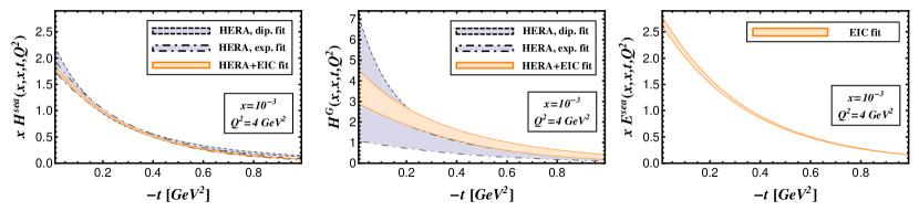
Figure 15: Least-squares fit extraction of sea quark GPD $H^{\rm sea}$ (left) and gluon GPD $H^{G}$ (middle) from a dipole ansatz (gray area surrounded by dashed curves) and an exponential ansatz (gray area surrounded by dashed-dotted curves) using only the HERA collider data. The results of a combined HERA/EIC fit including pseudo data for the unpolarized DVCS cross section, c.f. Fig. 13, and the transverse target spin asymmetry $A^{\sin(\phi-\phi_{S})}_{\rm UT}$, c.f. Fig. 14, using an exponential ansatz are shown as light orange area (surrounded by solid curves). In addition for the first time the sea quark GPD $E^{\rm sea}$ could be extracted (right panel).

In Fig. 15 we compare the resulting GPDs from fits to the HERA data alone and to the combined HERA+EIC data at ${\cal Q}^{2}=4\,\operatorname{GeV}^{2}$, $x_{\rm B}=10^{-3}$, and variable $-t$ (covering the HERA region). In the right panel one realizes that the uncertainty of the sea quark GPD $H^{\rm sea}$, which is to certain extent constrained by HERA data, can be strongly improved in particular at smaller $-t$ values. The gluon GPD $H^{G}$, displayed in the middle panel, is extracted by means of the ${\cal Q}^{2}$ evolution and it is rather weakly constrained by HERA DVCS data only. Here the inclusion of stage II EIC data yields a large improvement, even if the used lever arm in ${\cal Q}^{2}$, compared to HERA kinematics, is still rather limited. As emphasized above, information on the GPD $E$ can only be obtained from a new lepton-proton scattering experiment with a transversely polarized proton beam. In the right panel it is clearly demonstrated that the sea quark component of this GPD can be extracted with relatively small uncertainties. As explained above, from the utilized pseudo DVCS data the gluonic component of GPD $E$ (not shown) cannot be reliably accessed using our flexible GPD models.

5.2 Transverse spatial imaging

One of the main goals of GPD phenomenology is to provide the transverse spatial distributions of partons as function of the momentum fraction $x$. The simplest proposal to obtain a rough idea of such parton distributions is based on the Fourier transform of the amplitude Ralston:2001xs . Following the common experimental procedure one would extract the $t$-dependence from a fit to a given $(x_{\rm B},{\cal Q}^{2})$ bin. Utilizing the HERA data for DVCS and exclusive $J/\psi$ production and saying that the former process is quark dominated while the latter is gluon dominated, one immediately concludes from the experimental findings that the exponential $t$-slope parameter for DVCS cross section is larger than for the $J/\psi$ cross section,

$$B_{\rm DVCS}\approx 6\operatorname{GeV}^{-2}>B_{J/\psi}\approx 4\operatorname{GeV}^{-2}\,,$$

meaning that sea quarks are more spread out in transverse space than gluons. However, we may note that this rather generic interpretation is based on the assumption that the proton helicity non-conserved CFFs and/or amplitudes play no important role and that skewness effects are unimportant. We also emphasize that in a partonic interpretation the accessible lever arm in $-t$ is restricted by the DVCS requirement $-t\ll{\cal Q}^{2}$, which ensure that possible higher twist contributions, twist-four and higher, are small.

To quantify possible differences between a GPD interpretation and the aforementioned procedure, our GPD fit result from the preceding section is compared with (half of) the exponential $t$-slope of the differential DVCS cross section. The latter is extracted by fits to the $t$-dependence in a given $\{x_{\rm B},{\cal Q}^{2}\}$-bin of the pseudo data (5.1) by means of the exponential model

$$\frac{d\sigma_{i}^{\mbox{\tiny DVCS}}(t)}{dt}=n_{i}\;\exp\left\{2b_{i}\,t\right\}\,,$$ (57)

where $n_{i}$ and $b_{i}$ are the two fitting parameters used in bin $i$. The $\chi^{2}/{\rm d.o.f}$ value in these fits is usually around one, where the propagated standard error can be rather large for the lowest $x_{\rm B}$-bins, due to the BH subtraction procedure. From our GPD fit, we employ both the (sea) quark GPD $H$ on the cross-over line and the square root of the predicted differential DVCS cross section, the latter containing also additional contribution due to the non-vanishing CFF ${\cal E}$. ¿From both of these quantities we calculate an effective exponential $t$-slopes in the same manner. E.g., for the GPD on the cross-over line such a $t$-slope reads

$$b^{\rm eff}(x_{\rm B},{\cal Q}^{2})=\frac{1}{t_{2}-t_{1}}\ln\frac{H(x,x,t_{2},{\cal Q}^{2})}{H(x,x,t_{1},{\cal Q}^{2})}\quad$$ (58)

with $t_{1}=-0.03\,\operatorname{GeV}^{2}\,,\;\;t_{2}=-1.5\,\operatorname{GeV}^{2}\,,$ and $x=x_{\rm B}/(2-x_{\rm B})$.

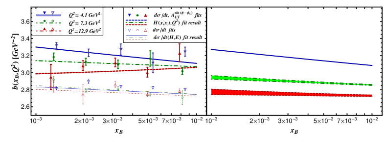
Figure 16: Exponential $t$-slope parameters from the model fit (57) to the DVCS cross section (empty symbols) and of $\Im{\rm m}{\cal H}$ from the model fit (59) to cross section and asymmetry data (filled symbols) as well as effective $t$-slope parameters (58), obtained from our GPD fit, for the GPD $H$ on the cross-over line (thick lines), the DVCS cross section prediction (thin lines), and the zero-skewness GPD $H$ (error bands in the right panel) are displayed as function of $x_{\rm B}$ for three different ${\cal Q}^{2}$ values: $4.1\operatorname{GeV}^{2}$ (triangles-down, solid curves, blue band), $7.3\operatorname{GeV}^{2}$ (circles, dash-dotted curves, green band), and $12.9\operatorname{GeV}^{2}$ (triangles-up, dashed curves, red band). Uncertainty bars arise from local fits to EIC pseudo data, while curves and uncertainty bands originate from a combined GPD model fit to HERA collider and EIC pseudo data.

In the left panel of Fig. 16 we show the results of the local exponential model (57) fits to the DVCS cross sections versus $x_{\rm B}$ for ${\cal Q}^{2}=4.1\operatorname{GeV}^{2}$, ${\cal Q}^{2}=7.3\operatorname{GeV}^{2}$, and ${\cal Q}^{2}=12.9\operatorname{GeV}^{2}$ as empty triangles-down, circles, and triangles-up, respectively. The effective $t$-slopes (58) of the GPD on the cross-over line, extracted from the combined GPD fit, are shown as thick solid, dash-dotted, and dashed curves, respectively, while effective $t$-slopes of GPD-fit-predicted cross sections are plotted as thin lines. Note that thick curves contain the uncertainty bands, arising from the propagation of pseudo data uncertainties. As one realizes, in our large $E$ scenario the $t$-slope of the DVCS cross section (57) is relatively flat w.r.t. both $x_{\rm B}$- and ${\cal Q}^{2}$-dependence, see empty symbols. This behavior differs drastically from that of the extracted GPD $H$ (thick curves), which has in addition also larger slope values. Nevertheless, the $b$-slope values extracted via exponential fit (57) are consistent with the effective DVCS cross section $t$-slope (thin curves), obtained from our GPD fit, and evaluated analogously to (58). In fact, the DVCS cross section (52) is in our model given as linear combination of two exponentials with different slope parameters. The behavior of GPD $H$ (left panel: thick curves) is partially compensated by the appearance of CFF ${\cal E}$. Note that for a small/vanishing GPD $E$ scenario these differences in the $b$-slope values would die out and the differences in the $t$-dependence of the CFF modulus $|{\cal H}|$ and $\Im{\rm m}{\cal H}$ can be considered to be small in the studied kinematical region. Consequently, under these circumstances and restricting the fits to LO accuracy, one can extract the $t$-dependence of GPD $H(x,x,t,{\cal Q}^{2})$ directly from the DVCS cross section measurements.

To go beyond the ${\cal H}$ dominance hypothesis in such cross section fits, one can utilize measurements of the single transverse proton spin asymmetry (53). We recall that this asymmetry is sensitive to CFF ${\cal E}$ and so the appropriate strategy is to use cross section and asymmetry data simultaneously in an analysis. To perform local fits for fixed $x_{\rm B}$ and ${\cal Q}^{2}$ one may set the real part of CFFs to zero. Alternatively, one can utilize a Regge-inspired ansatz, e.g., rather analogous as in (35), and perform fits for given ${\cal Q}^{2}$, see, e.g., Ref. FazFioJenLav11 . We performed such $2\times 4$ parameter ($n$, $\alpha(0)$, $\alpha^{\prime}$, $b$ for CFFs $\cal H$ and $\cal E$) fits in the three ${\cal Q}^{2}$ bins of the pseudo data sets (5.1) and (5.1). To compare the propagation of uncertainties with our local DVCS cross section fits, we used the extracted values for the two Regge trajectories $\alpha+\alpha^{\prime}t$ in local $2\times 2$ parameter fits to the EIC pseudo data. The $b$-slope parameters of the imaginary parts are defined as

$$\Im{\rm m}{\cal H}_{i}(t)=n_{i}\;\exp\left\{b_{i}\,t\right\}\quad\mbox{and}\quad\Im{\rm m}{\cal E}_{i}(t)=\overline{n}_{i}\;\exp\left\{\overline{b}_{i}\,t\right\}\,,$$ (59)

and the slightly $t$-dependent phase for a given $\{x_{\rm B},{\cal Q}^{2}\}$-bin $i$ was considered to be known. Furthermore, we restricted the set of asymmetry data (5.1) to those of the DVCS cross section (5.1). The results for the exponential $t$-slope parameter of $\Im{\rm m}{\cal H}$ are presented on the left panel in Fig. 16 as filled symbols for ${\cal Q}^{2}=4.1\operatorname{GeV}^{2}$ (triangle-down), ${\cal Q}^{2}=7.3\operatorname{GeV}^{2}$ (circle), and ${\cal Q}^{2}=12.9\operatorname{GeV}^{2}$ (triangle-up) and, as expected, they are compatible with the effective $t$-slope of the GPD $H(x,x,t,{\cal Q}^{2})$, extracted from our GPD fit (thick curves). However, the propagated uncertainties in these local fits are larger than in the previous ones, reflecting the fact that, particularly at larger $x_{\rm B}$, the asymmetry uncertainty can get large, see Fig. 14. Surely, assuming that both the assumed uncertainty distribution (Gaussian) and the model is correct, the uncertainty propagation in global fits, e.g., with a Regge-inspired ansatz, provides a much smaller error. It should be noted that both of these assumptions are only true with a certain probability.

Next we consider the effective $t$-slope, analogously defined as in (58), of the unpolarized quark GPD without skewness dependence,

$$q(x,t,{\cal Q}^{2})=H(x,\eta=0,t,{\cal Q}^{2}),$$ (60)

which is of great interest with regard to the transverse distribution of quarks. The result of our model is presented on the right panel of Fig. 16 and it can be compared to slopes of the GPD $H(x,\eta=x,t,{\cal Q}^{2})$ on the cross-over line in the left panel (thick lines). First it is observed that with growing ${\cal Q}^{2}$ not only the $x$-slope of the effective $t$-slope decreases as it is also seen for GPD $H(x,x,t,{\cal Q}^{2})$, but also its intercept drops. Loosely spoken, such a behavior means that both the “pomeron” slope parameter $\alpha^{\prime}$ and the value of the residual $t$-slope parameter decrease. This behavior of the zero-skewness GPD looks more natural and it is naively expected from the double log asymptotic behavior also for the GPD on the cross-over line Mue06 . However, with our AFKM12 model we illustrate by the thick curves in the left panel of Fig. 16 that specific choices of skewness parameters combined with $t$-slope parameters can provide also a rather flat effective residue dependence and a stronger decrease of the “pomeron” slope parameter $\alpha^{\prime}$. Since the $\eta\to 0$ limit commutes with the ${\cal Q}^{2}$-evolution, we conclude that evolution entangles the $t$-dependence with skewness dependence. Hence, the factorization of the $t$ and skewness dependence, assumed in our model at the initial scale, does not hold true under evolution (otherwise the effective slope parameters should evolve similarly). The reader might be also surprised that the uncertainty bands of the effective slope for the GPD on the cross over line remain tiny (thick curves on the left panel), while those in the forward (zero-skewness) case get sizable with increasing ${\cal Q}^{2}$ and decreasing $x$. This is caused by a naive truncation of the covariance matrix, i.e., removing rows and columns belonging to the skewness parameters $s_{2}$ and $s_{4}$ in the forward limit, which also alters the (anti)correlation of uncertainties that ensure the smallness of the uncertainties for GPD $H(x,x,t,{\cal Q}^{2})$. It is beyond the scope of this paper to study the uncertainties that arise from the extrapolation to $\eta\to 0$ in more depth, however, once high precision data will become available, one should also worry about the model bias in the extrapolation of GPD $F(x,\eta,t,{\cal Q}^{2})$ from $\eta=x$ to $\eta=0$.

Finally, we would like to illustrate that the EIC measurements of the $t$-dependence in the region $-t\lesssim 1.5\operatorname{GeV}^{2}$ can provide a probabilistic interpretation of the transverse distribution of sea quarks and partially also for gluons. The Fourier transform of the zero-skewness GPD (60) into the impact parameter space,

$$q(x,\vec{b},{\cal Q}^{2}) = \int\!\!\!\!\int_{-\infty}^{\infty}\!\frac{d^{2}\vec{\Delta}}{4\pi^{2}}\,e^{-i\vec{\Delta}\cdot\vec{b}}\,H(x,\eta=0,t=-\vec{\Delta}^{2},{\cal Q}^{2})$$

$$= \frac{1}{4\pi}\!\int_{0}^{\infty}\!\!\!d|t|\,J_{0}\!\left(b\sqrt{|t|}\right)\,H(x,\eta=0,t,{\cal Q}^{2})\,,$$

provides in the infinite momentum frame the probability of scattering on a quark as a function of its momentum fraction and transverse distance $b=|\vec{b}|$ from the proton center, where $1/{\cal Q}$ is considered as the resolution scale Burkardt:2000za . Since for an unpolarized struck quark and proton, no direction in the transverse plane is preferred, the integration over the polar angle in (5.2) yields a Bessel transform ($J_{k}(x)$ denotes the Bessel function of order $k$) and results in a parton density is symmetric under rotation of the two-dimensional impact parameter vector $\vec{b}$. For a transversely polarized proton, e.g., the polarization vector is pointing in the $x$ direction, one finds that the parton density is given by the unpolarized one (5.2) and a distortion in $y$ direction that is governed by the strength of GPD $E$,

$$q^{\Uparrow}(x,\vec{b},{\cal Q}^{2}) = q(x,\vec{b},{\cal Q}^{2})-\frac{1}{2M_{p}}\frac{\partial}{\partial b_{y}}E(x,\vec{b},{\cal Q}^{2})$$

$$= \frac{1}{4\pi}\!\int_{0}^{\infty}\!\!\!d|t|\!\left[\!J_{0}\!\left(b\sqrt{|t|}\right)H+\frac{b_{y}\sqrt{|t|}}{2bM_{p}}J_{1}\!\left(b\sqrt{|t|}\right)E\!\right]\!\!(x,\eta=0,t,{\cal Q}^{2})\,.$$

Before we present the resulting parton densities (5.2) from the combined GPD model fit to HERA and EIC pseudo data, let us shortly discuss the peculiarities in the uncertainty estimation. The uncertainty of the resulting parton densities is, besides the propagated experimental uncertainties, also dictated by the possible uncertainties caused by extrapolations from the accessible kinematical region, namely, (i) extrapolation of the skewness parameter dependence $\eta=x$ to $\eta=0$, discussed above, (ii) extrapolation of $t$-dependence from the experimental minimal $-t$ value $-t_{1}$ to $-t=0$, as well as (iii) from maximal accessible value $-t_{2}$ to $-t=\infty$. These rather intricate extrapolations are fortunately governed by the boundary condition,

$$q(x,{\cal Q}^{2})=H(x,\eta=0,t=0,{\cal Q}^{2})=\int\!\!\!\!\int_{-\infty}^{\infty}\!d^{2}\vec{b}\;q(x,\vec{b},{\cal Q}^{2}),$$ (63)

arising from the reduction of GPD $H$ in the kinematical forward limit to the standard unpolarized PDF $q$. Hence, the normalization of the (integrated) parton density (5.2) is also entirely determined by the PDF normalization. To simplify our study, we restrict ourselves to ${\cal Q}^{2}=4\operatorname{GeV}^{2}$, where in our model the $t$- and skewness dependencies factorize, as discussed above and exemplified also by the agreement of the effective slope parameters in the $\eta=x$ and $\eta=0$ case, see thick solid curves on the left and right panels on Fig. 16.

A model analysis studying the challenges of extrapolation in $-t$ beyond the experimentally accessible range has been presented for the differential cross section in AscDieFazINT2011 and we essentially agree with the conclusion that with an EIC imaging is feasible for $0.1\operatorname{fm}\lesssim b\lesssim 1.5\operatorname{fm}$ (or even in a wider range). Let us add some mathematical insight and let us point out methods to increase the quality of the extrapolations. With our model hypothesis the $t$-dependence of the zero-skewness GPD is essentially constrained by the EIC pseudo data in the region $0.03\operatorname{GeV}^{2}\leq-t\leq 1.5\operatorname{GeV}^{2}$.

The uncertainty of the extrapolation into the region $[0,-t_{1})$ is associated with the contribution

$$\Delta_{1}q(x,\vec{b},{\cal Q}^{2})=\frac{1}{4\pi}\!\int_{0}^{|t_{1}|}\!\!\!d|t|\,J_{0}\!\left(b\sqrt{|t|}\right)\,H(x,\eta=0,t,{\cal Q}^{2})\,,$$ (64)

from which one can easily obtain estimates. Although $q(x,{\cal Q}^{2})=H(x,\eta=0,t,{\cal Q}^{2})$ at $t=0$ is very well known, which makes this an interpolation problem rather then an extrapolation one, let us here calculate $\Delta_{1}q$ from the knowledge of $H$ in the vicinity of $-t_{1}$ by making use of a truncated Taylor series where the uncertainty is equated with the remainder. Consequently, to first order accuracy we have

$$\Delta_{1}q(x,\vec{b},{\cal Q}^{2}) \approx \frac{\sqrt{|t_{1}|}}{2\pi b}J_{1}\!\left(b|\sqrt{|t_{1}|}\right)\,H(x,0,t_{1},{\cal Q}^{2})+\frac{t_{1}}{\pi b^{2}}\frac{\sqrt{|t_{1}|}}{2\pi b}J_{2}\!\left(b|\sqrt{|t_{1}|}\right)\,\frac{d}{dt_{1}}H(x,0,t_{1},{\cal Q}^{2})\,,$$

$$\delta_{1}q(x,\vec{b},{\cal Q}^{2}) \approx \frac{2|t_{1}|^{3/2}}{\pi b^{3}}J_{3}\!\left(b\sqrt{|t_{1}|}\right)\,\frac{d^{2}}{dt^{2}_{1}}H(x,0,t_{1},{\cal Q}^{2})\,,$$ (65)

where the derivative of $H(x,0,t_{1},{\cal Q}^{2})$ can be evaluated numerically. For small $-t_{1}$ we can roughly estimate the value of the second order derivative in terms of the transverse width

$$\langle b^{2}\rangle(x,{\cal Q}^{2})=4\frac{d}{dt}\ln H(x,\eta=0,t,{\cal Q}^{2})\Big{|}_{t=0}\,,$$ (66)

e.g., for a $p$-pole ansatz we find

$$\frac{d^{2}}{dt^{2}_{1}}H(x,0,t_{1},{\cal Q}^{2})\approx\frac{1+p}{16p}\langle b^{2}\rangle^{2}(x,{\cal Q}^{2})q(x,{\cal Q}^{2})\,,$$

where the result for an exponentially functional form in $t$ follows from the limit $p\to\infty$. For a realistic value of $\langle\vec{b}^{2}\rangle\sim 0.35\,{\rm fm}^{2}$ in the small $x$ region, we find that the extrapolation uncertainty is of the order of $10^{-4}$ in units of $q(x,{\cal Q}^{2})/{\rm fm}^{2}$. However, this uncertainty becomes important in the large $b\gtrsim 1/\sqrt{|t_{1}|}\approx 1\operatorname{fm}$ region, dominated by the contributions from the small $-t$ region. Model analyzes provide a relative uncertainty on permill level for $b\approx 1\operatorname{fm}$, which, however, will increase to the few percent level for $b\approx 1.5\operatorname{fm}$ and will then grow fast for increasing $b$. Hence, with our EIC pseudo data we can resolve the transverse distribution up to a distance of $\approx 1.5\operatorname{fm}$. To estimate the uncertainty of the extrapolation into the $\{-t_{2},\infty]$ region we naively use

$$\Delta_{2}q(x,\vec{b},{\cal Q}^{2})=\frac{1}{4\pi}\!\int^{\infty}_{|t_{2}|}\!\!\!d|t|\,J_{0}(b\sqrt{|t|})\,H(x,\eta=0,t,{\cal Q}^{2})\,.$$ (67)

It is most important for the small-$b$ region, where in particular for $b=0$ we have

$$\Delta_{2}q(x,\vec{b}=0,{\cal Q}^{2})=\frac{1}{4\pi}\!\int^{\infty}_{|t_{2}|}\!\!\!d|t|\,H(x,\eta=0,t,{\cal Q}^{2})\,.$$ (68)

The relative uncertainty at $b=0$ is easily evaluated and we find for an exponential or $p$-pole form

$$\frac{\Delta_{2}q(x,\vec{b}=0,{\cal Q}^{2})}{q(x,\vec{b}=0,{\cal Q}^{2})}=e^{\langle b^{2}\rangle t_{2}/4}\quad\mbox{and}\quad\frac{\Delta_{2}q(x,\vec{b}=0,{\cal Q}^{2})}{q(x,\vec{b}=0,{\cal Q}^{2})}=\left(1-\frac{\langle b^{2}\rangle t_{2}}{4p}\right)^{-p+1}\,,$$

respectively. Assuming an exponential functional form it is with $-t_{2}\approx 1.5\operatorname{GeV}^{2}$ well under control and results in a $\sim 3\%$ correction, which, however, would increase for a dipole form to $\sim 40\%$. To reach the $10\%$ accuracy level, one must increase $-t_{2}\sim 8\operatorname{GeV}^{2}$, which requires a big ${\cal Q}^{2}$ value to ensure the validity of DVCS kinematics. Fortunately, the error, e.g., for $0.1\operatorname{fm}\leq b$, gets already on the $10\%$ level for $-t_{2}\sim 3.5\operatorname{GeV}^{2}$. Under these circumstances, one may rely on extrapolation techniques, e.g., based on conformal mapping or Padé approximation, to minimize the uncertainty. Note also that the uncertainty of extrapolation into the $\{-t_{2},\infty]$ region may be also associated with a relative uncertainty that grows fast with increasing $b$. In the following the uncertainty is calculated according to (68) and estimate numerically by assuming two alternative hypotheses, namely, that the $t$-dependence falls off exponentially or with $1/t^{2}$, where for a given $b$ value always the larger uncertainty is taken. For simplicity we will neglect the uncertainty from the extrapolation (interpolation) into the region $\{-t_{1},0]$, which is entirely justified for $b\leq 1\operatorname{fm}$ and as it would be hardly visible in the visualization of the parton densities for $b\leq 1.5\operatorname{fm}$. Finally, the uncertainty from the extrapolation into the large $-t$ region was added in quadrature to the one propagated from the (pseudo) data.

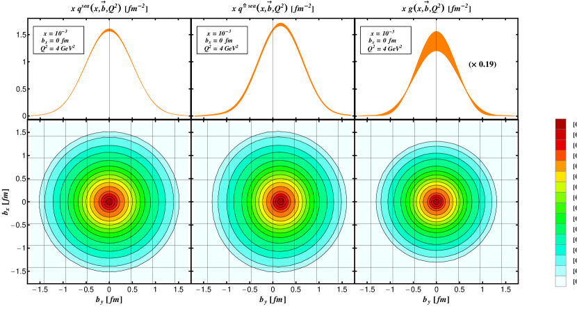
Figure 17: Parton densities at $x=0.001$ and ${\cal Q}^{2}=4\operatorname{GeV}^{2}$ versus impact parameter $b$ were obtained from a combined least-squares fit to the HERA collider and EIC pseudo data: relative densities (lower row) and their values at $b_{x}=0$ for the unpolarized sea quark parton densities of a unpolarized proton (left), a transversely polarized proton (middle), and the unpolarized gluon parton density of a unpolarized proton (right), its value is rescaled by a factor 0.19.

In the left and right columns on Fig. 17 the sea quark and gluon parton densities (5.2) at $x=10^{-3}$ and ${\cal Q}^{2}=4\operatorname{GeV}^{2}$ are shown as a relative density plot versus $b_{y}$ and $b_{x}$ (lower panels) and for $b_{x}=0$ as function of $b_{y}$ (upper panels). Note, the gluon density is rescaled by a factor of $0.19$. Since for sea quarks the propagated uncertainty is small and it was assumed that there is no cross-talk between $t$- and skewness dependencies, and the PDF uncertainties [fixed PDF parameters, see also boundary condition (63)] are neglected, the final uncertainties are smaller than for the corresponding $t$-dependent GPD at the cross-over line shown in the left panel of Fig. 15. Nevertheless, the increase of the uncertainty in the vicinity of $b=0$ due to the $\{-t_{2},\infty]$ extrapolation is visible for the quark density (upper left panel) and much more pronounced for the gluon density (upper right panel). Generally, the larger error for the gluon density is mainly based on the fact that the DVCS process alone does not allow to pin down this quantity on the same quantitative level as for sea quarks, see earlier discussions and Fig. 15. We again emphasize that the functional form of the $t$-dependence will influence the uncertainties related to the extrapolation error. For instance, a power-like falloff will increase the DVCS amplitude in the accessible large $-t$ region and therefore decrease the experimental uncertainties in this region, however, on the other hand, the uncertainties of the extrapolation into the $\{-t_{2},\infty]$ region will become more important.

Apart from the uncertainties that appear in the unpolarized parton densities, we also have the normalization uncertainty of GPD $E$, which is not protected by a boundary condition. Nevertheless, we found in our model that this uncertainty is not large. This is illustrated in the middle column of Fig. 17, where we display the sea quark density for a transversely polarized proton.

5.3 Angular momentum sum rule

Finally, we shortly discuss the role of the EIC measurements in elucidation of the Ji spin sum rule Ji:1996ek . This rule states that the proton spin

$$\frac{1}{2}=\sum_{q=u,d,s,\cdots}J^{q}({\cal Q}^{2})+J^{G}({\cal Q}^{2})$$ (69)

is built from quark and gluon angular momenta $J^{q}$ and $J^{G}$, which are defined via a gauge invariant decomposition of the QCD energy momentum tensor. Note that several other decompositions have been proposed, which are related to Ji‘s ones by reshuffling a certain amount of angular momentum fraction $\Delta J$, i.e.,

$$\sum_{q}J^{q}\Rightarrow\sum_{q}J^{q}+\Delta J\quad\mbox{and}\quad J^{G}\Rightarrow J^{G}-\Delta J\,,$$ (70)

where one may take the freedom to define $\Delta J$ as the expectation value of a gauge variant operator in order to reach a partonic interpretation of the gluon component in terms of spin and orbital angular momentum, e.g., to arrive at the Jaffe-Manohar spin sum rule Jaffe:1989jz . Ji‘s decomposition implies that the partonic components of the proton spin are given by the momentum fraction part, called here $A$, and the anomalous gravitomagnetic moment $B$,

$$J^{i}({\cal Q}^{2})=\frac{1}{2}A^{i}({\cal Q}^{2})+\frac{1}{2}B^{i}({\cal Q}^{2}),\quad\left\{{A\atop B}\right\}^{i}({\cal Q}^{2})=\int_{0}^{1}\!dx\,x\left\{{H\atop E}\right\}^{i}(x,\eta=0,t=0,{\cal Q}^{2})\,,$$ (71)

which are given by the first moments of GPDs $H$ and $E$, respectively. A phenomenological quantification of this sum rule is a highly intricate task, which is often trivialized by entirely relying on simple-minded GPD (or even transverse momentum dependent PDF) models or assumptions.

The definitions in Ji‘s angular momentum sum rule allow to employ any other QCD, i.e., field theory based framework to quantify the quark and gluon angular momenta. Most promising for achieving this goal are lattice gauge field simulations and once reliable results can be obtained, for a review see Hagler:2009ni , one may incorporate them in GPD models. There are various systematic uncertainties in the lattice estimation of angular momentum carried by sea quarks and gluons and hence their phenomenological determination is an important task for the future.

As we have seen, DVCS measurements at an EIC will allow to access the GPD $E$ at the cross-over line and allows, in a model dependent manner, to extract also its normalization in the forward kinematics. In fact, what we called anomalous magnetic moment of sea quarks is simply related to their angular momentum:

$$J^{\rm sea}=\frac{1}{2}\left(1+\kappa^{\rm sea}\right)A^{\rm sea}\,,$$

where the phenomenological value of the momentum fraction is at ${\cal Q}^{2}=4\operatorname{GeV}^{2}$ given by

$$A^{\rm sea}({\cal Q}^{2}=4\operatorname{GeV}^{2})\approx 0.15.$$

6 Summary

We show on some selected examples the physics case for DVCS measurements at a proposed EIC. Pseudo data were generated by the MC program MILOU that is tuned to HERA collider DVCS measurements. Full detector simulations have not yet been included; it was rather assumed that the systematical uncertainty for cross section measurements is on the 5% level. The statistical uncertainties of these simulations have been included in model predictions for various single spin asymmetries, electron charge asymmetries, and unpolarized cross sections, covering the EIC kinematics at stage I and II.

We illustrated that present GPD models, constrained by global fits to present DVCS data, provide a variety of EIC predictions, where in particular the $t$-dependence of the different models is poorly known and can be constrained to a large degree by EIC measurements. We did not discuss in completeness the extraction of CFFs, which can be done by having a polarized positron beam at hand. Here already a unpolarized one would help to have a cleaner access to twist-two associated CFFs. In particular, it can be used to isolate the interference term, which contains the most valuable information. This also provides an experimental cross-check for the smallness of the $\phi$-integrated interference term in cross section measurements. Rosenbluth separation, as it was worked out in Sect. 2.1, provides another handle on the isolation of BH and DVCS cross sections. This technique has to be explored further for the access of higher harmonics in the interference term. At present it is not known to what extent this method can be employed in a model independent manner, however, certainly it looks more intricate than in the case of unpolarized DIS or elastic form factor measurements.

While the access to CFFs and GPDs at lower beam energies requires the measurement of many observables the situation becomes simpler at higher energies. Here, we can assume that only two twist-two associated CFFs $\cal H$ and $\cal E$ show a “pomeron” behavior and are as such accessible in these kinematics. Moreover, their real parts are small compared to the imaginary and their phases are approximately given by an effective “pomeron” trajectory. Therefore, they can be accessed by a measurement of the DVCS cross section and the single transverse proton spin asymmetry. Thereby, at large electron energy loss $y$ and $-t$ the DVCS cross section may drop drastically and perhaps cannot be measured. In such circumstances one can use the single electron beam spin asymmetry measurements, which are predicted to be sizable at large $y$.

For parton imaging, it was illustrated that in a large GPD $E$ scenario its $t$-dependence extracted from the unpolarized cross section does not necessarily match the $t$-dependence of the sea quark GPD $H^{\rm sea}$. To extract in such a situation the $t$-dependence of CFFs $\cal H$ and $\cal E$ one may neglect the real part or use global fits, e.g., with a Regge-inspired ansatz in a given ${\cal Q}^{2}$ bin. Taking EIC pseudo data generated from MILOU and propagated to the predictions of AFKM12 model, we studied the error propagation to the sea quark and gluonic components of GPDs $H$ and $E$ by means of least-squares fits. Thereby, it turned out that with our rather flexible model the sea quark component of both GPDs can be pinned down quite precisely, while the knowledge of the gluon GPD $H^{\rm G}$ can also be substantially improved. However, the gluon GPD $E^{\rm G}$ is without further assumptions not accessible. To obtain a probabilistic interpretation, a model dependent extrapolation to the zero-skewness GPD has to be performed. We adopt in our studies the popular GPD model hypothesis that the skewness effect is $t$-independent, however, we also pointed out that this hypotheses may not hold under evolution. Certainly, this extrapolation may be considered as the largest theoretical uncertainty. Concerning the extrapolation uncertainties in the unmeasured $-t$ region, we found that the extrapolation into the small $-t$ region is well under control if the transverse resolution is of the order of $200\,{\rm MeV}$. This allows to resolve the transverse distribution of partons up to $1.5\operatorname{fm}$. In the case that the CFFs decrease strongly with increasing $-t$, e.g., exponentially, the experimentally accessible range, which overlaps with DVCS kinematics, is sufficient to provide an image of the sea quark GPDs $H$ and $E$ and also for the gluon GPD $H^{\rm G}$. If this will not be the case, the imaging procedure may not be under control if one simply neglects the non-accessible large $-t$ region. Under these circumstances one may increase experimentally the $-t$ range together with ${\cal Q}^{2}$ or employ mathematical extrapolation methods, which we did not explore here.

Let us also emphasize that the revealing of the CFF $\cal E$ in the small-$x_{\rm B}$ region is of more general interest, since it is loosely related to the problem whether the “pomeron” coupling can flip the spin of the proton. In the partonic language it is related to the question of whether sea quarks and gluons carry a non-vanishing gravitomagnetic moment or their angular momentum is simply given by half of their momentum fraction. Certainly the phenomenological access to this problem suffers from the uncertainties of extrapolation to the forward kinematics; however, the experimental measurement of CFF $\cal E$ can shed light on these questions, which at present can be hardly addressed with lattice gauge field simulations.

In summary, the proposed high-luminosity Electron Ion Collider, combined with its designated detector, would be an ideal apparatus for precise measurements of exclusive channels in both electron-proton and electron-nuclei scattering. Besides hard exclusive vector meson and photon electroproduction, one might address other exclusive channels, too. In particular, utilizing Monte-Carlo simulations and GPD fitting routines, we have shown the potential of such experiments for GPD phenomenology and the ability to obtain from such measurements the spatial distributions of sea quarks and gluons.

Appendix A Updates to the MILOU code

The MILOU code has been modified from its original version and it is currently maintained at BNL . The updates to the code mainly include bug fixing together with an improved output. The most relevant updates are the following:

• Bug fixed in the FORTRAN common blocks. Now they preserve the random seeds set in the cards and there is no need for recalculating the integral every event generation.

• The correct ALLM parametrization for the $F_{2}$ structure function has been implemented. This is relevant when running MILOU using the option for the Frankfurt-Freund-Strikman (FFS)FFS model, which computes the complex DVCS amplitude to LO and is not based on GPDs. Formerly, a wrong implementation of the ALLM parametrization caused a disagreement between the NLO GPD based and the FFS models. The correct ALLM is now taken from ALLM , and the agreement between the two models and with the predictions from the GenDVCS GenDVCS Monte Carlo (also using FFS) at HERA energies is satisfactory.

• A new output format. Beside the original output in the form of a PAW $n$-tuple PAW , a new output has been implemented in the form of a Pythia-like ascii format text file, in the same standard as other MCs used at EIC. A detailed description of the new output can be found on the web-page in footnote 11.

• Simulation of harmonics. In calculating the beam charge asymmetry, a functional form for the $cos(\phi)$ harmonic was formerly hard coded. Now the code points to the correct values from Freund/McDermott model.

• Simulation of the interference term. it is now properly set to the values expected from the Freund/McDermott model at NLO, without the twist-three contribution.

References

- (1) H1, C. Adloff et al., Phys. Lett. B517, 47 (2001), hep-ex/0107005.
- (2) ZEUS, S. Chekanov et al., Phys. Lett. B573, 46 (2003), hep-ex/0305028.
- (3) H1, A. Aktas et al., Eur. Phys. J. C44, 1 (2005), hep-ex/0505061.
- (4) H1, F. D. Aaron et al., Phys. Lett. B659, 796 (2008), 0709.4114 [hep-ex].
- (5) ZEUS, S. Chekanov et al., JHEP 05, 108 (2009), 0812.2517 [hep-ex].
- (6) H1, F. Aaron et al., Phys.Lett. B681, 391 (2009), 0907.5289 [hep-ex].
- (7) HERMES, A. Airapetian et al., Phys. Rev. D75, 011103 (2007), hep-ex/0605108.
- (8) HERMES, A. Airapetian et al., JHEP 06, 066 (2008), 0802.2499 [hep-ex].
- (9) HERMES, A. Airapetian et al., JHEP 11, 083 (2009), 0909.3587 [hep-ex].
- (10) HERMES, A. Airapetian et al., JHEP 06, 019 (2010), 1004.0177 [hep-ex].
- (11) HERMES, A. Airapetian et al., Phys. Lett. B704, 15 (2011), 1106.2990 [hep-ex].
- (12) HERMES, A. Airapetian et al., JHEP 1210, 042 (2012), 1206.5683 [hep-ex].
- (13) HERMES, A. Airapetian et al., JHEP 1207, 032 (2012), 1203.6287 [hep-ex].
- (14) CLAS, S. Chen et al., Phys. Rev. Lett. 97, 072002 (2006), hep-ex/0605012.
- (15) CLAS, F. X. Girod et al., Phys. Rev. Lett. 100, 162002 (2008), 0711.4805 [hep-ex].
- (16) CLAS, G. Gavalian et al., Phys. Rev. C80, 035206 (2009), 0812.2950 [hep-ex].
- (17) Jefferson Lab Hall A, C. M. Camacho et al., Phys. Rev. Lett. 97, 262002 (2006), nucl-ex/0607029.
- (18) Jefferson Lab Hall A, M. Mazouz et al., Phys. Rev. Lett. 99, 242501 (2007), 0709.0450 [nucl-ex].
- (19) H1, S. Aid et al., Nucl.Phys. B468, 3 (1996), hep-ex/9602007.
- (20) ZEUS, J. Breitweg et al., Eur. Phys. J. C6, 603 (1999), hep-ex/9808020.
- (21) H1, C. Adloff et al., Eur. Phys. J. C13, 371 (2000), hep-ex/9902019.
- (22) ZEUS, J. Breitweg et al., Eur. Phys. J. C12, 393 (2000), hep-ex/9908026.
- (23) H1, C. Adloff et al., Phys. Lett. B539, 25 (2002), hep-ex/0203022.
- (24) H1, F. D. Aaron et al., JHEP 05, 032 (2010), 0910.5831 [hep-ex].
- (25) ZEUS, S. Chekanov et al., PMC Phys. A1, 6 (2007), 0708.1478 [hep-ex].
- (26) HERMES, A. Airapetian et al., Eur. Phys. J. C17, 389 (2000), hep-ex/0004023.
- (27) HERMES, A. Airapetian et al., Eur. Phys. J. C71, 1609 (2011), 1012.3676 [hep-ex].
- (28) CLAS, C. Hadjidakis et al., Phys. Lett. B605, 256 (2005), hep-ex/0408005.
- (29) CLAS, S. A. Morrow et al., Eur. Phys. J. A39, 5 (2009), 0807.3834 [hep-ex].
- (30) ZEUS Collaboration, M. Derrick et al., Phys.Lett. B380, 220 (1996), hep-ex/9604008.
- (31) H1 Collaboration, C. Adloff et al., Z.Phys. C75, 607 (1997), hep-ex/9705014.
- (32) H1, C. Adloff et al., Phys. Lett. B483, 360 (2000), hep-ex/0005010.
- (33) ZEUS, S. Chekanov et al., Nucl. Phys. B718, 3 (2005), hep-ex/0504010.
- (34) HERMES, A. B. Borissov, Nucl. Phys. Proc. Suppl. 99A, 156 (2001).
- (35) CLAS, J. P. Santoro et al., Phys. Rev. C78, 025210 (2008), 0803.3537 [nucl-ex].
- (36) ZEUS, J. Breitweg et al., Phys. Lett. B487, 273 (2000), hep-ex/0006013.
- (37) CLAS, L. Morand et al., Eur. Phys. J. A24, 445 (2005), hep-ex/0504057.
- (38) H1, C. Adloff et al., Eur.Phys.J. C10, 373 (1999), hep-ex/9903008.
- (39) ZEUS, S. Chekanov et al., Nucl. Phys. B695, 3 (2004), hep-ex/0404008.
- (40) H1, A. Aktas et al., Eur. Phys. J. C46, 585 (2006), hep-ex/0510016.
- (41) H1, C. Adloff et al., Phys. Lett. B483, 23 (2000), hep-ex/0003020.
- (42) ZEUS, S. Chekanov et al., Phys.Lett. B680, 4 (2009), 0903.4205 [hep-ex].
- (43) ZEUS, H. Abramowicz et al., Phys.Lett. B708, 14 (2012), 1111.2133 [hep-ex].
- (44) HERMES, A. Airapetian et al., Phys. Lett. B659, 486 (2008), 0707.0222 [hep-ex].
- (45) Jefferson Lab Hall C, T. Horn et al., Phys. Rev. C78, 058201 (2008), 0707.1794 [nucl-ex].
- (46) Jefferson Lab Hall C, H. P. Blok et al., Phys. Rev. C78, 045202 (2008), 0809.3161 [nucl-ex].
- (47) A. Donnachie and P. Landshoff, Nucl.Phys. B231, 189 (1984).
- (48) J. P. Ralston and B. Pire, Phys. Rev. D66, 111501 (2002), hep-ph/0110075.
- (49) A. Donnachie and P. V. Landshoff, Phys. Lett. B437, 408 (1998), hep-ph/9806344.
- (50) I. I. Balitsky and L. N. Lipatov, Sov. J. Nucl. Phys. 28, 822 (1978).
- (51) E. A. Kuraev, L. N. Lipatov, and V. S. Fadin, Sov. Phys. JETP 45, 199 (1977).
- (52) A. H. Mueller and B. Patel, Nucl. Phys. B425, 471 (1994), hep-ph/9403256.
- (53) A. H. Mueller, Nucl. Phys. B415, 373 (1994).
- (54) L. D. McLerran and R. Venugopalan, Phys.Rev. D50, 2225 (1994), hep-ph/9402335.
- (55) E. Iancu, A. Leonidov, and L. D. McLerran, Nucl.Phys. A692, 583 (2001), hep-ph/0011241.
- (56) D. Müller, D. Robaschik, B. Geyer, F.-M. Dittes, and J. Hořejši, Fortschr. Phys. 42, 101 (1994), hep-ph/9812448.
- (57) A. V. Radyushkin, Phys. Lett. B380, 417 (1996), hep-ph/9604317.
- (58) X. Ji, Phys. Rev. D55, 7114 (1997), hep-ph/9609381.
- (59) A. V. Radyushkin, Phys. Rev. D58, 114008 (1998), hep-ph/9803316.
- (60) M. Diehl, T. Feldmann, R. Jakob, and P. Kroll, Eur. Phys. J. C8, 409 (1999), hep-ph/9811253.
- (61) S. V. Goloskokov and P. Kroll, Eur. Phys. J. C42, 281 (2005), hep-ph/0501242.
- (62) J. Collins, L. Frankfurt, and M. Strikman, Phys. Rev. D56, 2982 (1997), hep-ph/9611433.
- (63) J. Collins and A. Freund, Phys. Rev. D59, 074009 (1999), hep-ph/9801262.
- (64) M. Diehl, T. Feldmann, R. Jakob, and P. Kroll, Nucl. Phys. B596, 33 (2001), hep-ph/0009255, Erratum-ibid. B605 (2001) 647.
- (65) S. J. Brodsky, M. Diehl, and D. S. Hwang, Nucl. Phys. B596, 99 (2001), hep-ph/0009254.
- (66) M. Diehl, Phys. Rept. 388, 41 (2003), hep-ph/0307382.
- (67) A. V. Belitsky and A. V. Radyushkin, Phys. Rept. 418, 1 (2005), hep-ph/0504030.
- (68) M. Burkardt, Phys. Rev. D62, 071503 (2000), hep-ph/0005108, Erratum-ibid.D66:119903,2002.
- (69) M. Diehl, Eur. Phys. J. C25, 223 (2002), hep-ph/0205208, Erratum-ibid. C31 (2003) 277.
- (70) J. Kogut and D. Soper, Phys. Rev. D1, 2901 (1970).
- (71) X. Ji, Phys. Rev. Lett. 78, 610 (1997), hep-ph/9603249.
- (72) A. V. Belitsky, D. Müller, and A. Kirchner, Nucl. Phys. B629, 323 (2002), hep-ph/0112108.
- (73) A. Accardi, J. L. Albacete, M. Anselmino, N. Armesto, E. C. Aschenauer, A. Bacchetta, D. Boer and W. Brooks et al., (2012), 1212.1701 [nucl-ex].
- (74) A. V. Belitsky and D. Müller, Phys. Rev. D82, 074010 (2010), 1005.5209 [hep-ph].
- (75) A. V. Belitsky, D. Müller, and Y. Ji, (2012), 1212.6674 [hep-ph].
- (76) L. Hand, Phys.Rev. 129, 1834 (1963).
- (77) X. Ji, J. Phys. G24, 1181 (1998), hep-ph/9807358.
- (78) A. V. Radyushkin, Phys. Rev. D56, 5524 (1997), hep-ph/9704207.
- (79) A. D. Martin and M. G. Ryskin, Phys. Rev. D 57, 6692 (1998), hep-ph/9711371.
- (80) B. Pire, J. Soffer and O. Teryaev, Eur. Phys. J. C 8, 103 (1999), hep-ph/9804284.
- (81) A. V. Radyushkin, Phys. Rev. D 59, 014030 (1999), hep-ph/9805342.
- (82) X. -D. Ji, J. Phys. G 24, 1181 (1998), hep-ph/9807358.
- (83) P. Pobylitsa, Phys.Rev. D66, 094002 (2002), hep-ph/0204337.
- (84) P. V. Pobylitsa, Phys. Rev. D67, 094012 (2003), hep-ph/0210238.
- (85) P. V. Pobylitsa, Phys. Rev. D67, 034009 (2003), hep-ph/0210150.
- (86) X. Ji and J. Osborne, Phys. Rev. D58, 094018 (1998), hep-ph/9801260.
- (87) A. V. Belitsky and D. Müller, Phys. Lett. B417, 129 (1998), hep-ph/9709379.
- (88) L. Mankiewicz, G. Piller, E. Stein, M. Vänttinen, and T. Weigl, Phys. Lett. B425, 186 (1998), hep-ph/9712251.
- (89) X. Ji and J. Osborne, Phys. Rev. D 57, 1337 (1998), hep-ph/9707254.
- (90) A. V. Belitsky, A. Freund, and D. Müller, Nucl. Phys. B574, 347 (2000), hep-ph/9912379.
- (91) B. Pire, L. Szymanowski, and J. Wagner, Phys.Rev. D83, 034009 (2011), 1101.0555 [hep-ph].
- (92) D. Müller, Phys. Lett. B634, 227 (2006), hep-ph/0510109.
- (93) K. Kumerički, D. Müller, K. Passek-Kumerički, and A. Schäfer, Phys. Lett. B 648, 186 (2007), hep-ph/0605237.
- (94) V. M. Braun and A. N. Manashov, Phys. Rev. Lett. 107, 202001 (2011), 1108.2394 [hep-ph].
- (95) V. M. Braun and A. N. Manashov, JHEP 01, 085 (2012), 1111.6765 [hep-ph].
- (96) V. Braun, A. Manashov, and B. Pirnay, Phys.Rev. D86, 014003 (2012), 1205.3332 [hep-ph].
- (97) V. Braun, A. Manashov, and B. Pirnay, Phys. Rev. Lett. 109, 242001 (2012), 1209.2559 [hep-ph].
- (98) A. Belitsky and D. Müller, Phys. Lett. B486, 369 (2000), hep-ph/0005028.
- (99) N. Kivel and L. Mankiewicz, Eur. Phys. J. C21, 621 (2001), hep-ph/0106329.
- (100) O. V. Teryaev, Analytic properties of hard exclusive amplitudes, 2005, hep-ph/0510031.
- (101) M. V. Polyakov and C. Weiss, Phys. Rev. D60, 114017 (1999), hep-ph/9902451.
- (102) L. Mankiewicz, G. Piller, and A. Radyushkin, Eur. Phys. J. C 10, 307 (1999), hep-ph/9812467.
- (103) L. L. Frankfurt, M. V. Polyakov, M. Strikman, and M. Vanderhaeghen, Phys. Rev. Lett. 84, 2589 (2000), hep-ph/9911381.
- (104) C. Bechler and D. Müller, Generic modelling of non-perturbative quantities and a description of hard exclusive electroproduction (2009), 0906.2571 [hep-ph].
- (105) M. V. Polyakov and M. Vanderhaeghen, Taming Deeply Virtual Compton Scattering, 2008, 0803.1271 [hep-ph].
- (106) P. Kroll, H. Moutarde, and F. Sabatie, Eur. Phys. J. C 73, 2278 (2013), 1210.6975 [hep-ph].
- (107) L. L. Frankfurt, A. Freund, and M. Strikman, Phys. Rev. D 58, 114001 (1998), hep-ph/9710356, erratum D 59 (1999) 119901E.
- (108) K. Goeke, M. V. Polyakov, and M. Vanderhaeghen, Prog. Part. Nucl. Phys. 47, 401 (2001), hep-ph/0106012.
- (109) V. Guzey and T. Teckentrup, Phys. Rev. D74, 054027 (2006), hep-ph/0607099.
- (110) S. V. Goloskokov and P. Kroll, Eur. Phys. J. C53, 367 (2008), 0708.3569 [hep-ph].
- (111) S. V. Goloskokov and P. Kroll, Eur. Phys. J. C65, 137 (2010), 0906.0460 [hep-ph].
- (112) A. Freund and M. McDermott, Eur. Phys. J. C23, 651 (2002), hep-ph/0111472.
- (113) V. Guzey and T. Teckentrup, Phys. Rev. D79, 017501 (2009), 0810.3899 [hep-ph].
- (114) K. Kumerički and D. Müller, Nucl. Phys. B841, 1 (2010), 0904.0458 [hep-ph].
- (115) M. Guidal, Eur. Phys. J. A37, 319 (2008), 0807.2355 [hep-ph].
- (116) M. Guidal and H. Moutarde, Eur. Phys. J. A42, 71 (2009), 0905.1220 [hep-ph].
- (117) M. Guidal, Phys. Lett. B689, 156 (2010), 1003.0307 [hep-ph].
- (118) M. Guidal, Phys. Lett. B693, 17 (2010), 1005.4922 [hep-ph].
- (119) K. Kumerički, D. Müller, and A. Schäfer, JHEP 1107, 073 (2011), 1106.2808 [hep-ph].
- (120) K. Kumericki, D. Müller, and M. Murray, (2013), 1301.1230 [hep-ph].
- (121) K. Kumerički, D. Müller, and K. Passek-Kumerički, Eur. Phys. J. C58, 193 (2008), 0805.0152 [hep-ph].
- (122) A. V. Belitsky and D. Müller, Nucl. Phys. B589, 611 (2000), hep-ph/0007031.
- (123) K. Kumerički et al., (2011), 1105.0899 [hep-ph].
- (124) K. Kumerički and D. Müller, http://calculon.phy.hr/gpd/.
- (125) S. Goloskokov and P. Kroll, Eur.Phys.J. C59, 809 (2009), 0809.4126 [hep-ph].
- (126) S. Goloskokov and P. Kroll, Eur.Phys.J. A47, 112 (2011), 1106.4897 [hep-ph].
- (127) M. Meskauskas and D. Müller, (2011), 1112.2597 [hep-ph].
- (128) H. Moutarde, Phys. Rev. D79, 094021 (2009), 0904.1648 [hep-ph].
- (129) D. Boer, M. Diehl, R. Milner, R. Venugopalan, W. Vogelsang, D. Kaplan, H. Montgomery and S. Vigdor et al., Gluons and the quark sea at high energies: Distributions, polarization, tomography, 2011, 1108.1713 [nucl-th].
- (130) E. Perez, L. Schoeffel, and L. Favart, MILOU: A Monte-Carlo for deeply virtual Compton scattering, (2004), hep-ph/0411389.
- (131) A. Freund, M. McDermott, and M. Strikman, Phys. Rev. D67, 036001 (2003), hep-ph/0208160.
- (132) A. Freund, Phys.Rev. D68, 096006 (2003), hep-ph/0306012.
- (133) M. Diehl and D. Y. Ivanov, Eur. Phys. J. C52, 919 (2007), 0707.0351 [hep-ph].
- (134) A. Donnachie, Phys. Lett. B611, 255 (2005), hep-ph/0412085.
- (135) K. Kumerički, D. Müller, and K. Passek-Kumerički, (2007), 0710.5649 [hep-ph].
- (136) D. Müller, International Journal of Modern Physics: Conference Series 04, 168 (2011), http://www.worldscientific.com/doi/pdf/10.1142/S201019451100167X.
- (137) M. Penttinen, M. V. Polyakov, and K. Goeke, Phys. Rev. D62, 014024 (2000), hep-ph/9909489.
- (138) S. Alekhin, Phys. Rev. D68, 014002 (2003), hep-ph/0211096.
- (139) T. Gehrmann and W. J. Stirling, Phys. Rev. D53, 6100 (1996), hep-ph/9512406.
- (140) A. V. Belitsky, D. Müller, A. Kirchner, and A.Schäfer, Phys. Rev. D64, 116002 (2001), hep-ph/0011314.
- (141) E. R. Berger, F. Cano, M. Diehl, and B. Pire, Phys. Rev. Lett. 87, 142302 (2001), hep-ph/0106192.
- (142) A. Kirchner and D. Müller, Eur. Phys. J. C32, 347 (2003), hep-ph/0302007.
- (143) F. Cano and B. Pire, Eur. Phys. J. A19, 423 (2004), hep-ph/0307231.
- (144) D. Y. Ivanov, L. Szymanowski, and G. Krasnikov, JETP Lett. 80, 226 (2004), hep-ph/0407207, Pisma Zh. Eksp. Teor. Fiz 80 (2004) 255.
- (145) E. R. Berger, M. Diehl, and B. Pire, Eur. Phys. J. C23, 675 (2001), hep-ph/0110062.
- (146) H. Moutarde, B. Pire, F. Sabatie, L. Szymanowski, and J. Wagner, Phys. Rev. D87, 054029 (2103), 1301.3819 [hep-ph].
- (147) M. Guidal and M. Vanderhaeghen, Phys. Rev. Lett. 90, 012001 (2003), hep-ph/0208275.
- (148) A. V. Belitsky and D. Müller, Phys. Rev. Lett. 90, 022001 (2003), hep-ph/0210313.
- (149) A. V. Belitsky and D. Müller, Phys. Rev. D68, 116005 (2003), hep-ph/0307369.
- (150) M. Diehl, How large can the distributions and be?, in Gluons and the quark sea at high energies: Distributions, polarization, tomography., 2011, 1108.1713 [nucl-th].
- (151) S. Fazio, R. Fiore, L. Jenkovszky, and A. Lavorini, Phys. Rev. D 85, 054009 (2012).
- (152) D. Müller, Pomeron dominance in deeply virtual Compton scattering and the femto holographic image of the proton, 2006, hep-ph/0605013.
- (153) E.-C. Aschenauer, M. Diehl, and S. Fazio, From transverse-momentum spectra to transverse images, in Gluons and the quark sea at high energies: Distributions, polarization, tomography., 2011, 1108.1713 [nucl-th].
- (154) R. Jaffe and A. Manohar, Nucl.Phys. B337, 509 (1990), Revised version.
- (155) P. Hagler, Phys. Rept. 490, 49 (2010), 0912.5483 [hep-lat].
- (156) L. Frankfurt, A. Freund, M. Strikman, Phys. Lett. B 460, 417 (1999).
- (157) H. Abramowicz, A. Levy, The ALLM parameterization of : An Update, hep-ph/9712415.
- (158) P. R. B. Saull, A Monte Carlo Generator for Deeply Virtual Compton Scattering at HERA, 1999, available on-line at http://wwwzeus.desy.de/physics/diff/pub/MC.
- (159) PAW - Physics Analysis Workstation, available on-line at http://paw.web.cern.ch/paw/