Inversion of moments to retrieve joint probabilities in quantum sequential measurements

H. S. Karthik Raman Research Institute, Bangalore 560 080, India    Hemant Katiyar Department of Physics and NMR Research Center, Indian Institute of Science Education and Research, Pune 411008, India    Abhishek Shukla Department of Physics and NMR Research Center, Indian Institute of Science Education and Research, Pune 411008, India    A. R. Usha Devi Department of Physics, Bangalore University, Bangalore-560 056, India Inspire Institute Inc., Alexandria, Virginia, 22303, USA. arutth@rediffmail.com    A. K. Rajagopal Inspire Institute Inc., Alexandria, Virginia, 22303, USA. Harish-Chandra Research Institute, Chhatnag Road, Jhunsi, Allahabad 211 019, India.    T. S. Mahesh Department of Physics and NMR Research Center, Indian Institute of Science Education and Research, Pune 411008, India
Abstract

A sequence of moments obtained from statistical trials encodes a classical probability distribution. However, it is well-known that an incompatible set of moments arise in the quantum scenario, when correlation outcomes associated with measurements on spatially separated entangled states are considered. This feature viz., the incompatibility of moments with a joint probability distribution is reflected in the violation of Bell inequalities. Here, we focus on sequential measurements on a single quantum system and investigate if moments and joint probabilities are compatible with each other. By considering sequential measurement of a dichotomic dynamical observable at three different time intervals, we explicitly demonstrate that the moments and the probabilities are inconsistent with each other. Experimental results using a nuclear magnetic resonance (NMR) system are reported here to corroborate these theoretical observations viz., the incompatibility of the three-time joint probabilties with those extracted from the moment sequence when sequential measurements on a single qubit system are considered.

Joint probabilities, Sequential measurement, Moments
pacs:
03.65.Ta, 03.67.Lx

I Introduction

The issue of determining a probability distribution uniquely in terms of its moment sequence – known as classical moment problem – has been developed for more than 100 years Tamarkin ; Akhiezer . In the case of discrete distributions with the associated random variables taking finite values, moments faithfully capture the essence of the probabilities i.e., the probability distribution is moment determinate Shi .

In the special case of classical random variables Xisubscript𝑋𝑖X_{i} assuming dichotomic values xi=±1subscript𝑥𝑖plus-or-minus1x_{i}=\pm 1, it is easy to see that the sequence of moments note1 μn1n2nk=X1n1X2n2Xknk=x1,x2,xk=±1x1n1x2n2xknkP(x1,x2,,xk),subscript𝜇subscript𝑛1subscript𝑛2subscript𝑛𝑘delimited-⟨⟩superscriptsubscript𝑋1subscript𝑛1superscriptsubscript𝑋2subscript𝑛2superscriptsubscript𝑋𝑘subscript𝑛𝑘subscriptsubscript𝑥1subscript𝑥2subscript𝑥𝑘plus-or-minus1subscriptsuperscript𝑥subscript𝑛11subscriptsuperscript𝑥subscript𝑛22subscriptsuperscript𝑥subscript𝑛𝑘𝑘𝑃subscript𝑥1subscript𝑥2subscript𝑥𝑘\mu_{n_{1}\,n_{2}\,\ldots n_{k}}=\langle X_{1}^{n_{1}}X_{2}^{n_{2}}\ldots X_{k}^{n_{k}}\rangle=\displaystyle{\sum_{x_{1},x_{2},\ldots\,x_{k}=\pm 1}}\,x^{n_{1}}_{1}\,x^{n_{2}}_{2}\ldots\,x^{n_{k}}_{k}\,P(x_{1},x_{2},\ldots,x_{k})\ , where n1,n2,,nk=0,1,formulae-sequencesubscript𝑛1subscript𝑛2subscript𝑛𝑘01n_{1},n_{2},\ldots,n_{k}=0,1, can be readily inverted to obtain the joint probabilities P(x1,x2,,xk)𝑃subscript𝑥1subscript𝑥2subscript𝑥𝑘P(x_{1},x_{2},\ldots,x_{k}) uniquely. More explicitly, the joint probabilities P(x1,x2,,xk)𝑃subscript𝑥1subscript𝑥2subscript𝑥𝑘P(x_{1},x_{2},\ldots,x_{k}) are given in terms of the 2ksuperscript2𝑘2^{k} moments μn1n2nk,n1,n2,nk=0,1formulae-sequencesubscript𝜇subscript𝑛1subscript𝑛2subscript𝑛𝑘subscript𝑛1subscript𝑛2subscript𝑛𝑘01\mu_{n_{1}\,n_{2}\,\ldots n_{k}},n_{1},n_{2},\ldots n_{k}=0,1 as,

P(x1,x2,,xk)=12kn1,nk=0,1x1n1x2n2xknkμn1nk𝑃subscript𝑥1subscript𝑥2subscript𝑥𝑘1superscript2𝑘subscriptformulae-sequencesubscript𝑛1subscript𝑛𝑘01superscriptsubscript𝑥1subscript𝑛1superscriptsubscript𝑥2subscript𝑛2superscriptsubscript𝑥𝑘subscript𝑛𝑘subscript𝜇subscript𝑛1subscript𝑛𝑘\displaystyle P(x_{1},x_{2},\ldots,x_{k})=\frac{1}{2^{k}}\sum_{n_{1},\ldots n_{k}=0,1}\,x_{1}^{n_{1}}x_{2}^{n_{2}}\ldots x_{k}^{n_{k}}\,\mu_{n_{1}\,\ldots n_{k}}
=12kn1,,nk=0,1x1n1x2n2xknkX1n1X2n2X2nk.absent1superscript2𝑘subscriptformulae-sequencesubscript𝑛1subscript𝑛𝑘01superscriptsubscript𝑥1subscript𝑛1superscriptsubscript𝑥2subscript𝑛2superscriptsubscript𝑥𝑘subscript𝑛𝑘delimited-⟨⟩superscriptsubscript𝑋1subscript𝑛1superscriptsubscript𝑋2subscript𝑛2superscriptsubscript𝑋2subscript𝑛𝑘\displaystyle=\frac{1}{2^{k}}\,\sum_{n_{1},\ldots,n_{k}=0,1}\,x_{1}^{n_{1}}x_{2}^{n_{2}}\ldots x_{k}^{n_{k}}\,\langle X_{1}^{n_{1}}X_{2}^{n_{2}}\ldots X_{2}^{n_{k}}\rangle.

Does this feature prevail in the quantum scenario? This results in a negative answer as it is wellknown that the moments associated with measurement outcomes on spatially separated parties are not compatible with the joint probability distribution. This feature reflects itself in the violation of Bell inequalities. In this paper we investigate whether moment-indeterminacy persists when we focus on sequential measurements on a single quantum system. We show that the discrete joint probabilities originating in the sequential measurement of a single qubit dichotomic observable X^(ti)=X^i^𝑋subscript𝑡𝑖subscript^𝑋𝑖\hat{X}(t_{i})=\hat{X}_{i} at different time intervals are not consistent with the ones reconstructed from the moments. More explicitly, considering sequential measurements of X^1subscript^𝑋1\hat{X}_{1}, X^2subscript^𝑋2\hat{X}_{2}, X^3subscript^𝑋3\hat{X}_{3}, we reconstruct the trivariate joint probabilties Pμ(x1,x2,x3)subscript𝑃𝜇subscript𝑥1subscript𝑥2subscript𝑥3P_{\mu}(x_{1},x_{2},x_{3}) based on the set of eight moments {X^1,X^2,X^3,X^1X^2,X^2X^3,X^1X^3,X^1X^2X^3}delimited-⟨⟩subscript^𝑋1delimited-⟨⟩subscript^𝑋2delimited-⟨⟩subscript^𝑋3delimited-⟨⟩subscript^𝑋1subscript^𝑋2delimited-⟨⟩subscript^𝑋2subscript^𝑋3delimited-⟨⟩subscript^𝑋1subscript^𝑋3delimited-⟨⟩subscript^𝑋1subscript^𝑋2subscript^𝑋3\{\langle\hat{X}_{1}\rangle,\langle\hat{X}_{2}\rangle,\langle\hat{X}_{3}\rangle,\langle\hat{X}_{1}\,\hat{X}_{2}\rangle,\langle\hat{X}_{2}\,\hat{X}_{3}\rangle,\langle\hat{X}_{1}\,\hat{X}_{3}\rangle,\langle\hat{X}_{1}\,\hat{X}_{2}\,\hat{X}_{3}\rangle\} and prove that they do not agree with the three-time joint probabilities (TTJP) Pd(x1,x2,x3)subscript𝑃𝑑subscript𝑥1subscript𝑥2subscript𝑥3P_{d}(x_{1},x_{2},x_{3}) evaluated directly based on the correlation outcomes in the sequential measurement of all the three observables. Interestingly, the moments and TTJP can be independently extracted experimentally in NMR system – demonstrating the difference between moment inverted three time probabilities with the ones directly drawn from experiment, in agreement with theory. For obtaining TTJP directly we use the procedure of Ref. nmr_elgi and for extracting moments we extend the Moussa protocol Moussa to a set of non-commutating observables. The specifics are given in the experimental section.

Disagreement between moment inverted joint probabilities with the ones based on measurement outcomes in turn reflects the inherent inconsistency that the family of all marginal probabilities do not arise from the grand joint probabilities. The non-existence of a legitimate grand joint probability distribution, consistent with the set of all pairwise marginals is attributed to be the common origin of a wide range of no-go theorems on non-contextuality, locality and macrorealism in the foundations of quantum theory Fine ; Bell ; KS ; Peres ; Mermin ; LG ; UKSR ; TP2013 . The absence of a valid grand joint probability distribution in the sequential measurement on a single quantum system is brought out here in terms of its mismatch with moment sequence.

We organize the paper as follows. In Sec. II we begin with a discussion on moment inversion to obtain joint probabilities of three classical random variables assuming dichotomic values ±1plus-or-minus1\pm 1. We proceed in Sec. III to study the quantum scenario with the help of a specific example of sequential measurements of dichotomic observable at three different times on a spin-1/2 system. We show that the TTJP constructed from eight moments do not agree with those originated from the measurement outcomes. Sec. IV is devoted to report experimental results with NMR implementation on an ensemble of spin-1/2 nuclei, demonstrating that moment constructed TTJP do not agree with those directly extracted. Section V has concluding remarks.

II Reconstruction of joint probability of classical dichotomic random variables from moments

Let X𝑋X denote a dichotomic random variable with outcomes x=±1𝑥plus-or-minus1x=\pm 1. The moments associated with statistical outcomes involving the variable X𝑋X are given by μn=Xn=x=±1xnP(x),n=0,1,2,3,formulae-sequencesubscript𝜇𝑛delimited-⟨⟩superscript𝑋𝑛subscript𝑥plus-or-minus1superscript𝑥𝑛𝑃𝑥𝑛0123\mu_{n}=\langle X^{n}\rangle=\sum_{x=\pm 1}x^{n}\,P(x),\ n=0,1,2,3,\ldots, where 0P(x=±1)1;x=±1P(x)=1formulae-sequence0𝑃𝑥plus-or-minus11subscript𝑥plus-or-minus1𝑃𝑥10\leq P(x=\pm 1)\leq 1;\sum_{x=\pm 1}P(x)=1 are the corresponding probabilities. Given the moments μ0subscript𝜇0\mu_{0} and μ1subscript𝜇1\mu_{1} from a statistical trial, one can readily obtain the probability mass function:

P(1)𝑃1\displaystyle P(1) =\displaystyle= 12(μ0+μ1)=12(1+μ1)12subscript𝜇0subscript𝜇1121subscript𝜇1\displaystyle\frac{1}{2}(\mu_{0}+\mu_{1})=\frac{1}{2}(1+\mu_{1})
P(1)𝑃1\displaystyle P(-1) =\displaystyle= 12(μ0μ1)=12(1μ1),12subscript𝜇0subscript𝜇1121subscript𝜇1\displaystyle\frac{1}{2}(\mu_{0}-\mu_{1})=\frac{1}{2}(1-\mu_{1}),

i.e., moments determine the probabilities uniquely.

In the case of two dichotomic random variables X1subscript𝑋1X_{1}, X2subscript𝑋2X_{2}, the moments μn1,n2=X1n1X2n2=x1=±1,x2=±1x1n1x2n2P(x1,x2),n1,n2=0,1formulae-sequencesubscript𝜇subscript𝑛1subscript𝑛2delimited-⟨⟩superscriptsubscript𝑋1subscript𝑛1superscriptsubscript𝑋2subscript𝑛2subscriptformulae-sequencesubscript𝑥1plus-or-minus1subscript𝑥2plus-or-minus1superscriptsubscript𝑥1subscript𝑛1superscriptsubscript𝑥2subscript𝑛2𝑃subscript𝑥1subscript𝑥2subscript𝑛1subscript𝑛201\mu_{n_{1},n_{2}}=\langle X_{1}^{n_{1}}\,X_{2}^{n_{2}}\rangle=\displaystyle\sum_{x_{1}=\pm 1,x_{2}=\pm 1}\,x_{1}^{n_{1}}\,x_{2}^{n_{2}}\,P(x_{1},x_{2}),\ n_{1},n_{2}=0,1\ldots encode the bivariate probabilities P(x1,x2)𝑃subscript𝑥1subscript𝑥2P(x_{1},x_{2}). Explicitly,

μ00subscript𝜇00\displaystyle\mu_{00} =\displaystyle= x1,x2=±1P(x1,x2)=P(1,1)+P(1,1)+P(1,1)+P(1,1)=1,subscriptsubscript𝑥1subscript𝑥2plus-or-minus1𝑃subscript𝑥1subscript𝑥2𝑃11𝑃11𝑃11𝑃111\displaystyle\sum_{x_{1},x_{2}=\pm 1}\,P(x_{1},x_{2})=P(1,1)+P(1,-1)+P(-1,1)+P(-1,-1)=1,
μ10subscript𝜇10\displaystyle\mu_{10} =\displaystyle= x1,x2=±1x1P(x1,x2)=x1=±1x1P(x1),subscriptsubscript𝑥1subscript𝑥2plus-or-minus1subscript𝑥1𝑃subscript𝑥1subscript𝑥2subscriptsubscript𝑥1plus-or-minus1subscript𝑥1𝑃subscript𝑥1\displaystyle\sum_{x_{1},x_{2}=\pm 1}\,x_{1}\,P(x_{1},x_{2})=\sum_{x_{1}=\pm 1}\,x_{1}\,\,P(x_{1}),
=\displaystyle= P(1,1)+P(1,1)P(1,1)P(1,1)𝑃11𝑃11𝑃11𝑃11\displaystyle P(1,1)+P(1,-1)-P(-1,1)-P(-1,-1)
μ01subscript𝜇01\displaystyle\mu_{01} =\displaystyle= x1,x2=±1x2P(x1,x2)=x2x2P(x2)subscriptsubscript𝑥1subscript𝑥2plus-or-minus1subscript𝑥2𝑃subscript𝑥1subscript𝑥2subscriptsubscript𝑥2subscript𝑥2𝑃subscript𝑥2\displaystyle\sum_{x_{1},x_{2}=\pm 1}x_{2}\,P(x_{1},x_{2})=\sum_{x_{2}}\,x_{2}\,P(x_{2})
=\displaystyle= P(1,1)P(1,1)+P(1,1)P(1,1)𝑃11𝑃11𝑃11𝑃11\displaystyle P(1,1)-P(1,-1)+P(-1,1)-P(-1,-1)
μ11subscript𝜇11\displaystyle\mu_{11} =\displaystyle= x1,x2=±1x1x2P(x1,x2)=P(1,1)P(1,1)P(1,1)+P(1,1).subscriptsubscript𝑥1subscript𝑥2plus-or-minus1subscript𝑥1subscript𝑥2𝑃subscript𝑥1subscript𝑥2𝑃11𝑃11𝑃11𝑃11\displaystyle\sum_{x_{1},x_{2}=\pm 1}\,x_{1}\,x_{2}\,P(x_{1},x_{2})=P(1,1)-P(1,-1)-P(-1,1)+P(-1,-1). (2)

Note that the moments μ10subscript𝜇10\mu_{10}, μ01subscript𝜇01\mu_{01} involve the marginal probabilities P(x1)=x2=±1P(x1,x2)𝑃subscript𝑥1subscriptsubscript𝑥2plus-or-minus1𝑃subscript𝑥1subscript𝑥2P(x_{1})=\sum_{x_{2}=\pm 1}\,P(x_{1},x_{2}), P(x2)=x1=±1P(x1,x2)𝑃subscript𝑥2subscriptsubscript𝑥1plus-or-minus1𝑃subscript𝑥1subscript𝑥2P(x_{2})=\sum_{x_{1}=\pm 1}\,P(x_{1},x_{2}) respectively and they could be evaluated based on statistical trials drawn independently from the two random variables X1subscript𝑋1X_{1} and X2subscript𝑋2X_{2}.

Given the moments μ00,μ10,μ01,μ11subscript𝜇00subscript𝜇10subscript𝜇01subscript𝜇11\mu_{00},\mu_{10},\mu_{01},\mu_{11} the reconstruction of the probabilities P(x1,x2)𝑃subscript𝑥1subscript𝑥2P(x_{1},x_{2}) is straightforward:

P(x1,x2)𝑃subscript𝑥1subscript𝑥2\displaystyle P(x_{1},x_{2}) =\displaystyle= 14n1,n2=0,1x1n1x2n2μn1n214subscriptformulae-sequencesubscript𝑛1subscript𝑛201superscriptsubscript𝑥1subscript𝑛1superscriptsubscript𝑥2subscript𝑛2subscript𝜇subscript𝑛1subscript𝑛2\displaystyle\frac{1}{4}\,\sum_{n_{1},n_{2}=0,1}\,x_{1}^{n_{1}}x_{2}^{n_{2}}\,\mu_{n_{1}\,n_{2}} (3)
=\displaystyle= 14n1,n2=0,1x1n1x2n2X1n1X2n2.14subscriptformulae-sequencesubscript𝑛1subscript𝑛201superscriptsubscript𝑥1subscript𝑛1superscriptsubscript𝑥2subscript𝑛2delimited-⟨⟩superscriptsubscript𝑋1subscript𝑛1superscriptsubscript𝑋2subscript𝑛2\displaystyle\frac{1}{4}\,\sum_{n_{1},n_{2}=0,1}\,x_{1}^{n_{1}}x_{2}^{n_{2}}\,\langle X_{1}^{n_{1}}\,X_{2}^{n_{2}}\rangle.

Further, a reconstruction of trivariate joint probabilities P(x1,x2,x3)𝑃subscript𝑥1subscript𝑥2subscript𝑥3P(x_{1},x_{2},x_{3}) requires the following set of eight moments: {μ000=1,μ100=X1,μ010=X2,μ010=X3,μ110=X1X2,μ011=X2X3,μ101=X1X3,μ111=X1X2X3}formulae-sequencesubscript𝜇0001formulae-sequencesubscript𝜇100delimited-⟨⟩subscript𝑋1formulae-sequencesubscript𝜇010delimited-⟨⟩subscript𝑋2formulae-sequencesubscript𝜇010delimited-⟨⟩subscript𝑋3formulae-sequencesubscript𝜇110delimited-⟨⟩subscript𝑋1subscript𝑋2formulae-sequencesubscript𝜇011delimited-⟨⟩subscript𝑋2subscript𝑋3formulae-sequencesubscript𝜇101delimited-⟨⟩subscript𝑋1subscript𝑋3subscript𝜇111delimited-⟨⟩subscript𝑋1subscript𝑋2subscript𝑋3\{\mu_{000}=1,\mu_{100}=\langle X_{1}\rangle,\ \mu_{010}=\langle X_{2}\rangle,\mu_{010}=\langle X_{3}\rangle,\mu_{110}=\langle X_{1}\,X_{2}\rangle,\mu_{011}=\langle X_{2}\,X_{3}\rangle,\mu_{101}=\langle X_{1}\,X_{3}\rangle,\ \mu_{111}=\langle X_{1}\,X_{2}\,X_{3}\rangle\}. The probabilities are retrieved faithfully in terms of the eight moments as,

P(x1,x2,x3)=18n1,n2,n3=0,1x1n1x2n2x3n3μn1n2n3𝑃subscript𝑥1subscript𝑥2subscript𝑥318subscriptformulae-sequencesubscript𝑛1subscript𝑛2subscript𝑛301superscriptsubscript𝑥1subscript𝑛1superscriptsubscript𝑥2subscript𝑛2superscriptsubscript𝑥3subscript𝑛3subscript𝜇subscript𝑛1subscript𝑛2subscript𝑛3\displaystyle P(x_{1},x_{2},x_{3})=\frac{1}{8}\,\sum_{n_{1},n_{2},n_{3}=0,1}\,x_{1}^{n_{1}}x_{2}^{n_{2}}x_{3}^{n_{3}}\,\mu_{n_{1}\,n_{2}\,n_{3}}
=18n1,n2,n3=0,1x1n1x2n2x3n3X1n1X2n2X3n3.absent18subscriptformulae-sequencesubscript𝑛1subscript𝑛2subscript𝑛301superscriptsubscript𝑥1subscript𝑛1superscriptsubscript𝑥2subscript𝑛2superscriptsubscript𝑥3subscript𝑛3delimited-⟨⟩superscriptsubscript𝑋1subscript𝑛1superscriptsubscript𝑋2subscript𝑛2subscriptsuperscript𝑋subscript𝑛33\displaystyle=\frac{1}{8}\,\sum_{n_{1},n_{2},n_{3}=0,1}\,x_{1}^{n_{1}}x_{2}^{n_{2}}x_{3}^{n_{3}}\,\langle X_{1}^{n_{1}}\,X_{2}^{n_{2}}\,X^{n_{3}}_{3}\rangle.

It is implicit that the moments μ100,μ010,μ001subscript𝜇100subscript𝜇010subscript𝜇001\mu_{100},\mu_{010},\mu_{001} are determined through independent statistical trials involving the random variables X1,X2,X3subscript𝑋1subscript𝑋2subscript𝑋3X_{1},X_{2},X_{3} separately; μ110,μ011,μ101subscript𝜇110subscript𝜇011subscript𝜇101\mu_{110},\mu_{011},\mu_{101} are obtained based on the correlation outcomes of (X1,X2)subscript𝑋1subscript𝑋2(X_{1},X_{2}), (X2,X3)subscript𝑋2subscript𝑋3(X_{2},X_{3}) and (X1,X3)subscript𝑋1subscript𝑋3(X_{1},X_{3}) respectively. More specifically, in the classical probability setting there is a tacit underlying assumption that the set of all marginal probabilities P(x1),P(x2),P(x3),P(x1,x2),P(x2,x3),P(x1,x3)𝑃subscript𝑥1𝑃subscript𝑥2𝑃subscript𝑥3𝑃subscript𝑥1subscript𝑥2𝑃subscript𝑥2subscript𝑥3𝑃subscript𝑥1subscript𝑥3P(x_{1}),P(x_{2}),P(x_{3}),P(x_{1},x_{2}),P(x_{2},x_{3}),P(x_{1},x_{3}) are consistent with the trivariate joint probabilities P(x1,x2,x3)𝑃subscript𝑥1subscript𝑥2subscript𝑥3P(x_{1},x_{2},x_{3}). This underpinning does not get imprinted automatically in the quantum scenario. Suppose the observables X^1,X^2,X^3subscript^𝑋1subscript^𝑋2subscript^𝑋3\hat{X}_{1},\hat{X}_{2},\hat{X}_{3} are non-commuting and we consider their sequential measurement. The moments μ100=X^1,μ010=X^2,μ001=X^3formulae-sequencesubscript𝜇100delimited-⟨⟩subscript^𝑋1formulae-sequencesubscript𝜇010delimited-⟨⟩subscript^𝑋2subscript𝜇001delimited-⟨⟩subscript^𝑋3\mu_{100}=\langle\hat{X}_{1}\rangle,\mu_{010}=\langle\hat{X}_{2}\rangle,\ \mu_{001}=\langle\hat{X}_{3}\rangle may be evaluated from the measurement outcomes of dichotomic observables X^1,X^2,X^3subscript^𝑋1subscript^𝑋2subscript^𝑋3\hat{X}_{1},\hat{X}_{2},\hat{X}_{3} independently; the correlated statistical outcomes in the sequential measurements of (X^1,X^2)subscript^𝑋1subscript^𝑋2(\hat{X}_{1},\ \hat{X}_{2}), (X^2,X^3)subscript^𝑋2subscript^𝑋3(\hat{X}_{2},\ \hat{X}_{3}) and (X^1,X^3)subscript^𝑋1subscript^𝑋3(\hat{X}_{1},\ \hat{X}_{3}) allow one to extract the set of moments μ110=X^1X^2,μ011=X^2X^3,μ101=X^1X^3formulae-sequencesubscript𝜇110delimited-⟨⟩subscript^𝑋1subscript^𝑋2formulae-sequencesubscript𝜇011delimited-⟨⟩subscript^𝑋2subscript^𝑋3subscript𝜇101delimited-⟨⟩subscript^𝑋1subscript^𝑋3\mu_{110}=\langle\hat{X}_{1}\hat{X}_{2}\rangle,\ \mu_{011}=\langle\hat{X}_{2}\hat{X}_{3}\rangle,\mu_{101}=\langle\,\hat{X}_{1}\hat{X}_{3}\rangle; further the moment μ111=X^1X^2X^3subscript𝜇111delimited-⟨⟩subscript^𝑋1subscript^𝑋2subscript^𝑋3\mu_{111}=\langle\hat{X}_{1}\,\hat{X}_{2}\,\hat{X}_{3}\rangle is evaluated based on the correlation outcomes when all the three observables are measured sequentially. The joint probabilities Pμ(x1,x2,x3)subscript𝑃𝜇subscript𝑥1subscript𝑥2subscript𝑥3P_{\mu}(x_{1},x_{2},x_{3}) retrieved from the moments as given in (II) differ from the ones evaluated directly in terms of the correlation outcomes in the sequential measurement of all the three observables . We illustrate this inconsistency appearing in the quantum setting in the next section.

III Quantum three-time joint probabilities and moment inversion

Let us consider a spin-1/2 system, dynamical evolution of which is governed by the Hamiltonian

H^=12ωσx.^𝐻12Planck-constant-over-2-pi𝜔subscript𝜎𝑥\hat{H}=\frac{1}{2}\,\hbar\,\omega\sigma_{x}. (5)

We choose z-component of spin as our dynamical observable:

X^isubscript^𝑋𝑖\displaystyle\hat{X}_{i} =\displaystyle= X^(ti)=σz(ti)^𝑋subscript𝑡𝑖subscript𝜎𝑧subscript𝑡𝑖\displaystyle\hat{X}(t_{i})=\sigma_{z}(t_{i}) (6)
=\displaystyle= U^(ti)σzU^(ti)superscript^𝑈subscript𝑡𝑖subscript𝜎𝑧^𝑈subscript𝑡𝑖\displaystyle\hat{U}^{\dagger}(t_{i})\,\sigma_{z}\,\hat{U}(t_{i})
=\displaystyle= σzcosωti+σysinωti,subscript𝜎𝑧𝜔subscript𝑡𝑖subscript𝜎𝑦𝜔subscript𝑡𝑖\displaystyle\sigma_{z}\,\cos\omega\,t_{i}+\sigma_{y}\,\sin\omega\,t_{i},

where U^(ti)=eiσxωti/2=U^i^𝑈subscript𝑡𝑖superscript𝑒𝑖subscript𝜎𝑥𝜔subscript𝑡𝑖2subscript^𝑈𝑖\hat{U}(t_{i})=e^{-i\,\sigma_{x}\,\omega\,t_{i}/2}=\hat{U}_{i}, and consider sequential measurements of the observable X^isubscript^𝑋𝑖\hat{X}_{i} at three different times t1=0,t2=Δt,t3=2Δtformulae-sequencesubscript𝑡10formulae-sequencesubscript𝑡2Δ𝑡subscript𝑡32Δ𝑡t_{1}=0,t_{2}=\Delta t,t_{3}=2\,\Delta t:

X^1subscript^𝑋1\displaystyle\hat{X}_{1} =\displaystyle= σzsubscript𝜎𝑧\displaystyle\sigma_{z}
X^2subscript^𝑋2\displaystyle\hat{X}_{2} =\displaystyle= σz(Δt)=σzcos(ωΔt)+σysin(ωΔt)subscript𝜎𝑧Δ𝑡subscript𝜎𝑧𝜔Δ𝑡subscript𝜎𝑦𝜔Δ𝑡\displaystyle\sigma_{z}(\Delta t)=\sigma_{z}\,\cos(\omega\Delta t)+\sigma_{y}\,\sin(\omega\Delta t)
X^3subscript^𝑋3\displaystyle\hat{X}_{3} =\displaystyle= σz(2Δt)=σzcos(2ωΔt)+σysin(2ωΔt).subscript𝜎𝑧2Δ𝑡subscript𝜎𝑧2𝜔Δ𝑡subscript𝜎𝑦2𝜔Δ𝑡\displaystyle\sigma_{z}(2\Delta t)=\sigma_{z}\,\cos(2\omega\Delta t)+\sigma_{y}\,\sin(2\omega\Delta t). (7)

Note that these three operators are not commuting in general.

The moments X^1,X^2,X^3delimited-⟨⟩subscript^𝑋1delimited-⟨⟩subscript^𝑋2delimited-⟨⟩subscript^𝑋3\langle\hat{X}_{1}\rangle,\langle\hat{X}_{2}\rangle,\langle\hat{X}_{3}\rangle are readily evaluated to be

μ100subscript𝜇100\displaystyle\mu_{100} =\displaystyle= X^1=Tr[ρ^inσz]=0,delimited-⟨⟩subscript^𝑋1Trdelimited-[]subscript^𝜌insubscript𝜎𝑧0\displaystyle\langle\hat{X}_{1}\rangle={\rm Tr}[\hat{\rho}_{\rm in}\,\sigma_{z}]=0,
μ010subscript𝜇010\displaystyle\mu_{010} =\displaystyle= X^2=Tr[ρ^inσz(Δt)]=0,delimited-⟨⟩subscript^𝑋2Trdelimited-[]subscript^𝜌insubscript𝜎𝑧Δ𝑡0\displaystyle\langle\hat{X}_{2}\rangle={\rm Tr}[\hat{\rho}_{\rm in}\,\sigma_{z}(\Delta t)]=0,
μ001subscript𝜇001\displaystyle\mu_{001} =\displaystyle= X^3=Tr[ρ^inσz(2Δt)]=0.delimited-⟨⟩subscript^𝑋3Trdelimited-[]subscript^𝜌insubscript𝜎𝑧2Δ𝑡0\displaystyle\langle\hat{X}_{3}\rangle={\rm Tr}[\hat{\rho}_{\rm in}\,\sigma_{z}(2\Delta t)]=0.

when the system density matrix is prepared initially in a maximally mixed state ρ^in=𝟙/2subscript^𝜌in12\hat{\rho}_{\rm in}=\mathbbm{1}/2. The probabilities of outcomes xi=±1subscript𝑥𝑖plus-or-minus1x_{i}=\pm 1 in the completely random initial state are given by P(xi=±1)=Tr[ρ^inΠ^xi]=12𝑃subscript𝑥𝑖plus-or-minus1Trdelimited-[]subscript^𝜌insubscript^Πsubscript𝑥𝑖12P(x_{i}=\pm 1)={\rm Tr}[\hat{\rho}_{\rm in}\,\hat{\Pi}_{x_{i}}]=\frac{1}{2}, where Π^xi=|xixi|subscript^Πsubscript𝑥𝑖ketsubscript𝑥𝑖brasubscript𝑥𝑖\hat{\Pi}_{x_{i}}=|x_{i}\rangle\langle x_{i}| is the projection operator corresponding to measurement of the observable X^isubscript^𝑋𝑖\hat{X}_{i}.

The two-time joint probabilities arising in the sequential measurements of the observables X^i,X^j,j>isubscript^𝑋𝑖subscript^𝑋𝑗𝑗𝑖\hat{X}_{i},\hat{X}_{j},\ j>i are evaluated as follows. The measurement of the observable X^isubscript^𝑋𝑖\hat{X}_{i} yielding the outcome xi=±1subscript𝑥𝑖plus-or-minus1x_{i}=\pm 1 projects the the density operator to ρ^xi=Π^xiρ^inΠ^xiTr[ρ^inΠ^xi]subscript^𝜌subscript𝑥𝑖subscript^Πsubscript𝑥𝑖subscript^𝜌insubscript^Πsubscript𝑥𝑖Trdelimited-[]subscript^𝜌insubscript^Πsubscript𝑥𝑖\hat{\rho}_{x_{i}}=\frac{\hat{\Pi}_{x_{i}}\,\hat{\rho}_{\rm in}\,\hat{\Pi}_{x_{i}}}{{\rm Tr}[\hat{\rho}_{\rm in}\,\hat{\Pi}_{x_{i}}]}. Further, a sequential measurement of X^jsubscript^𝑋𝑗\hat{X}_{j} leads to the two-time joint probabilities as,

P(xi,xj)𝑃subscript𝑥𝑖subscript𝑥𝑗\displaystyle P(x_{i},x_{j}) =\displaystyle= P(xi)P(xj|xi)𝑃subscript𝑥𝑖𝑃conditionalsubscript𝑥𝑗subscript𝑥𝑖\displaystyle P(x_{i})\,P(x_{j}|x_{i}) (8)
=\displaystyle= Tr[ρ^inΠ^xi]Tr[ρ^xiΠ^xj]Trdelimited-[]subscript^𝜌insubscript^Πsubscript𝑥𝑖Trdelimited-[]subscript^𝜌subscript𝑥𝑖subscript^Πsubscript𝑥𝑗\displaystyle{\rm Tr}[\hat{\rho}_{\rm in}\,\hat{\Pi}_{x_{i}}]\ {\rm Tr}[\hat{\rho}_{x_{i}}\,\hat{\Pi}_{x_{j}}]
=\displaystyle= Tr[Π^xiρ^inΠ^xiΠ^xj]Trdelimited-[]subscript^Πsubscript𝑥𝑖subscript^𝜌insubscript^Πsubscript𝑥𝑖subscript^Πsubscript𝑥𝑗\displaystyle{\rm Tr}[\hat{\Pi}_{x_{i}}\,\hat{\rho}_{\rm in}\,\hat{\Pi}_{x_{i}}\hat{\Pi}_{x_{j}}]
=\displaystyle= xi|ρ^in|xi|xi|xj|2quantum-operator-productsubscript𝑥𝑖subscript^𝜌insubscript𝑥𝑖superscriptinner-productsubscript𝑥𝑖subscript𝑥𝑗2\displaystyle\langle x_{i}|\,\hat{\rho}_{\rm in}\,|x_{i}\rangle\,|\langle x_{i}|x_{j}\rangle|^{2}

We evaluate the two-time joint probabilities associated with the sequential measurements of (X^1,X^2)subscript^𝑋1subscript^𝑋2(\hat{X}_{1},\hat{X}_{2}), (X^2,X^3)subscript^𝑋2subscript^𝑋3(\hat{X}_{2},\hat{X}_{3}), and (X^1,X^3)subscript^𝑋1subscript^𝑋3(\hat{X}_{1},\hat{X}_{3}) explicitly:

P(x1,x2)=14[1+x1x2cos(ωΔt)]𝑃subscript𝑥1subscript𝑥214delimited-[]1subscript𝑥1subscript𝑥2𝜔Δ𝑡\displaystyle P(x_{1},x_{2})=\frac{1}{4}\,[1+x_{1}\,x_{2}\,\cos(\omega\Delta t)] (9)
P(x2,x3)=14[1+x2x3cos(ωΔt)]𝑃subscript𝑥2subscript𝑥314delimited-[]1subscript𝑥2subscript𝑥3𝜔Δ𝑡\displaystyle P(x_{2},x_{3})=\frac{1}{4}\,[1+x_{2}\,x_{3}\,\cos(\omega\Delta t)] (10)
P(x1,x3)=14[1+x1x3cos(2ωΔt)].𝑃subscript𝑥1subscript𝑥314delimited-[]1subscript𝑥1subscript𝑥32𝜔Δ𝑡\displaystyle P(x_{1},x_{3})=\frac{1}{4}\,[1+x_{1}\,x_{3}\,\cos(2\omega\Delta t)]. (11)

We then obtain two-time correlation moments as,

μ110=X^1X^2subscript𝜇110delimited-⟨⟩subscript^𝑋1subscript^𝑋2\displaystyle\mu_{110}=\langle\,\hat{X}_{1}\hat{X}_{2}\rangle =\displaystyle= x1,x2=±1x1x2P(x1,x2)subscriptsubscript𝑥1subscript𝑥2plus-or-minus1subscript𝑥1subscript𝑥2𝑃subscript𝑥1subscript𝑥2\displaystyle\sum_{x_{1},x_{2}=\pm 1}\,x_{1}\,x_{2}\,P(x_{1},x_{2}) (12)
=\displaystyle= cos(ωΔt)𝜔Δ𝑡\displaystyle\cos(\omega\Delta t)
μ011=X^2X^3subscript𝜇011delimited-⟨⟩subscript^𝑋2subscript^𝑋3\displaystyle\mu_{011}=\langle\,\hat{X}_{2}\hat{X}_{3}\rangle =\displaystyle= x2,x3=±1x2x3P(x2,x3)subscriptsubscript𝑥2subscript𝑥3plus-or-minus1subscript𝑥2subscript𝑥3𝑃subscript𝑥2subscript𝑥3\displaystyle\sum_{x_{2},x_{3}=\pm 1}\,x_{2}\,x_{3}\,P(x_{2},x_{3}) (13)
=\displaystyle= cos(ωΔt)𝜔Δ𝑡\displaystyle\cos(\omega\Delta t)
μ101=X^1X^3subscript𝜇101delimited-⟨⟩subscript^𝑋1subscript^𝑋3\displaystyle\mu_{101}=\langle\,\hat{X}_{1}\hat{X}_{3}\rangle =\displaystyle= x1,x3=±1x1x3P(x1,x3)subscriptsubscript𝑥1subscript𝑥3plus-or-minus1subscript𝑥1subscript𝑥3𝑃subscript𝑥1subscript𝑥3\displaystyle\sum_{x_{1},x_{3}=\pm 1}\,x_{1}\,x_{3}\,P(x_{1},x_{3}) (14)
=\displaystyle= cos(2ωΔt).2𝜔Δ𝑡\displaystyle\cos(2\,\omega\Delta t).

Further, the three-time joint probabilities P(x1,x2,x3)𝑃subscript𝑥1subscript𝑥2subscript𝑥3P(x_{1},x_{2},x_{3}) arising in the sequential measurements of X^1,X^2subscript^𝑋1subscript^𝑋2\hat{X}_{1},\hat{X}_{2}, followed by X^3subscript^𝑋3\hat{X}_{3} are given by

P(x1,x2,x3)𝑃subscript𝑥1subscript𝑥2subscript𝑥3\displaystyle P(x_{1},x_{2},x_{3}) =\displaystyle= P(x1)P(x2|x1)P(x3|x1,x2)𝑃subscript𝑥1𝑃conditionalsubscript𝑥2subscript𝑥1𝑃conditionalsubscript𝑥3subscript𝑥1subscript𝑥2\displaystyle P(x_{1})\,P(x_{2}|x_{1})\,P(x_{3}|x_{1},x_{2})
=\displaystyle= Tr[ρ^inΠ^x1]Tr[ρ^x1Π^x2]Tr[ρ^x2Π^x3]Trdelimited-[]subscript^𝜌insubscript^Πsubscript𝑥1Trdelimited-[]subscript^𝜌subscript𝑥1subscript^Πsubscript𝑥2Trdelimited-[]subscript^𝜌subscript𝑥2subscript^Πsubscript𝑥3\displaystyle{\rm Tr}[\hat{\rho}_{\rm in}\,\hat{\Pi}_{x_{1}}]\,{\rm Tr}[\hat{\rho}_{x_{1}}\,\hat{\Pi}_{x_{2}}]\,{\rm Tr}[\hat{\rho}_{x_{2}}\,\hat{\Pi}_{x_{3}}]

where ρ^x2=Π^x2ρ^x1Π^x2Tr[ρ^x1Π^x2].subscript^𝜌subscript𝑥2subscript^Πsubscript𝑥2subscript^𝜌subscript𝑥1subscript^Πsubscript𝑥2Trdelimited-[]subscript^𝜌subscript𝑥1subscript^Πsubscript𝑥2\hat{\rho}_{x_{2}}=\frac{\hat{\Pi}_{x_{2}}\,\hat{\rho}_{x_{1}}\,\hat{\Pi}_{x_{2}}}{{\rm Tr}[\hat{\rho}_{x_{1}}\,\hat{\Pi}_{x_{2}}]}. We obtain,

P(x1,x2,x3)𝑃subscript𝑥1subscript𝑥2subscript𝑥3\displaystyle P(x_{1},x_{2},x_{3}) =\displaystyle= Tr[Π^x2Π^x1ρ^inΠ^x1Π^x2Π^x3]Trdelimited-[]subscript^Πsubscript𝑥2subscript^Πsubscript𝑥1subscript^𝜌insubscript^Πsubscript𝑥1subscript^Πsubscript𝑥2subscript^Πsubscript𝑥3\displaystyle{\rm Tr}[\hat{\Pi}_{x_{2}}\,\hat{\Pi}_{x_{1}}\,\hat{\rho}_{\rm in}\,\hat{\Pi}_{x_{1}}\,\hat{\Pi}_{x_{2}}\,\hat{\Pi}_{x_{3}}] (16)
=\displaystyle= x1|ρ^in|x1|x1|x2|2|x2|x3|2quantum-operator-productsubscript𝑥1subscript^𝜌insubscript𝑥1superscriptinner-productsubscript𝑥1subscript𝑥22superscriptinner-productsubscript𝑥2subscript𝑥32\displaystyle\langle x_{1}|\,\hat{\rho}_{\rm in}\,|x_{1}\rangle\,|\langle x_{1}|x_{2}\rangle|^{2}\,|\langle x_{2}|x_{3}\rangle|^{2}
=\displaystyle= P(x1,x2)P(x2,x3)x2|ρ^in|x2𝑃subscript𝑥1subscript𝑥2𝑃subscript𝑥2subscript𝑥3quantum-operator-productsubscript𝑥2subscript^𝜌insubscript𝑥2\displaystyle\frac{P(x_{1},x_{2})\,P(x_{2},x_{3})}{\langle x_{2}|\,\hat{\rho}_{\rm in}\,|x_{2}\rangle}
=\displaystyle= P(x1,x2)P(x2,x3)P(x2)𝑃subscript𝑥1subscript𝑥2𝑃subscript𝑥2subscript𝑥3𝑃subscript𝑥2\displaystyle\frac{P(x_{1},x_{2})\,P(x_{2},x_{3})}{P(x_{2})}

where in the third line of (16) we have used (8).

The three-time correlation moment is evaluated to be,

μ111=X^1X^2X^3subscript𝜇111delimited-⟨⟩subscript^𝑋1subscript^𝑋2subscript^𝑋3\displaystyle\mu_{111}=\langle\hat{X}_{1}\,\hat{X}_{2}\,\hat{X}_{3}\rangle =\displaystyle= x1,x2,x3=±1x1x2x3P(x1,x2,x3)subscriptsubscript𝑥1subscript𝑥2subscript𝑥3plus-or-minus1subscript𝑥1subscript𝑥2subscript𝑥3𝑃subscript𝑥1subscript𝑥2subscript𝑥3\displaystyle\sum_{x_{1},x_{2},x_{3}=\pm 1}\,x_{1}\,x_{2}\,x_{3}\,P(x_{1},x_{2},x_{3}) (17)
=\displaystyle= 0.0\displaystyle 0.

From the set of eight moments (III), (12) and (17), we construct the TTJP (see (II)) as,

Pμ(1,1,1)subscript𝑃𝜇111\displaystyle P_{\mu}(1,1,1) =\displaystyle= 18[1+2cos(ωΔt)+cos(2ωΔt)]=Pμ(1,1,1),18delimited-[]12𝜔Δ𝑡2𝜔Δ𝑡subscript𝑃𝜇111\displaystyle\frac{1}{8}\ [1+2\cos(\omega\Delta t)+\cos(2\omega\Delta t)]=P_{\mu}(-1,-1,-1),
Pμ(1,1,1)subscript𝑃𝜇111\displaystyle P_{\mu}(-1,1,1) =\displaystyle= 18[1cos(2ωΔt)]=Pμ(1,1,1)=Pμ(1,1,1)=Pμ(1,1,1),18delimited-[]12𝜔Δ𝑡subscript𝑃𝜇111subscript𝑃𝜇111subscript𝑃𝜇111\displaystyle\frac{1}{8}\ [1-\cos(2\omega\Delta t)]=P_{\mu}(-1,-1,1)=P_{\mu}(1,1,-1)=P_{\mu}(1,-1,-1), (18)
Pμ(1,1,1)subscript𝑃𝜇111\displaystyle P_{\mu}(1,-1,1) =\displaystyle= 18[12cos(ωΔt)+cos(2ωΔt)]=Pμ(1,1,1).18delimited-[]12𝜔Δ𝑡2𝜔Δ𝑡subscript𝑃𝜇111\displaystyle\frac{1}{8}\ [1-2\cos(\omega\Delta t)+\cos(2\omega\Delta t)]=P_{\mu}(-1,1,-1).

On the other hand, the three dichotomic variable quantum probabilities P(x1,x2,x3)𝑃subscript𝑥1subscript𝑥2subscript𝑥3P(x_{1},x_{2},x_{3}) evaluated directly are given by,

Pd(1,1,1)subscript𝑃𝑑111\displaystyle P_{d}(1,1,1) =\displaystyle= 18[1+cos(ωΔt)]2=Pd(1,1,1),18superscriptdelimited-[]1𝜔Δ𝑡2subscript𝑃𝑑111\displaystyle\frac{1}{8}\,[1+\cos(\omega\,\Delta t)]^{2}=P_{d}(-1,-1,-1),
Pd(1,1,1)subscript𝑃𝑑111\displaystyle P_{d}(-1,1,1) =\displaystyle= 18[1cos2(ωΔt)]=Pd(1,1,1)=Pd(1,1,1)=Pd(1,1,1),18delimited-[]1superscript2𝜔Δ𝑡subscript𝑃𝑑111subscript𝑃𝑑111subscript𝑃𝑑111\displaystyle\frac{1}{8}\,[1-\cos^{2}(\omega\,\Delta t)]=P_{d}(-1,-1,1)=P_{d}(1,1,-1)=P_{d}(1,-1,-1), (19)
Pd(1,1,1)subscript𝑃𝑑111\displaystyle P_{d}(1,-1,1) =\displaystyle= 18[1cos(ωΔt)]2=Pd(1,1,1).18superscriptdelimited-[]1𝜔Δ𝑡2subscript𝑃𝑑111\displaystyle\frac{1}{8}\,[1-\cos(\omega\,\Delta t)]^{2}=P_{d}(-1,1,-1).

Clearly, there is no agreement between the moment inverted TTJP (III) and the ones of (III) directly evaluated. In other words, the TTJP realized in a sequential measurement are not invertible in terms of the moments – which in turn reflects the incompatibility of the set of all marginal probabilities with the grand joint probabilities Pd(x1,x2,x3).subscript𝑃𝑑subscript𝑥1subscript𝑥2subscript𝑥3P_{d}(x_{1},x_{2},x_{3}). In fact, it may be explicitly verified that P(x1,x3)x2=±1Pd(x1,x2,x3).𝑃subscript𝑥1subscript𝑥3subscriptsubscript𝑥2plus-or-minus1subscript𝑃𝑑subscript𝑥1subscript𝑥2subscript𝑥3P(x_{1},x_{3})\neq\sum_{x_{2}=\pm 1}\,P_{d}(x_{1},x_{2},x_{3}). Moment-indeterminacy points towards the absence of a valid grand probability distribution consistent with all the marginals.

The TTJP and moments can be independently extracted experimentally using NMR methods on an ensemble of spin-1/2 nuclei. The experimental approach and results are reported in the next section.

IV Experiment

The projection operators at time t=0𝑡0t=0 (X^1=σzsubscript^𝑋1subscript𝜎𝑧\hat{X}_{1}=\sigma_{z}) are {Π^xi0=|xi0xi0|}xi0=0,1subscriptsubscript^Πsubscriptsuperscript𝑥0𝑖ketsubscriptsuperscript𝑥0𝑖brasubscriptsuperscript𝑥0𝑖subscriptsuperscript𝑥0𝑖01\{\hat{\Pi}_{x^{0}_{i}}=|{x^{0}_{i}}\rangle\langle{x^{0}_{i}}|\}_{x^{0}_{i}=0,1}. This measurement basis is rotating under the unitary U^isubscript^𝑈𝑖\hat{U}_{i}, resulting in time dependent basis given by, Π^xit=U^iΠ^xi0U^isubscript^Πsuperscriptsubscript𝑥𝑖𝑡subscriptsuperscript^𝑈𝑖subscript^Πsubscriptsuperscript𝑥0𝑖subscript^𝑈𝑖\hat{\Pi}_{x_{i}^{t}}=\hat{U}^{\dagger}_{i}\,\hat{\Pi}_{x^{0}_{i}}\hat{U}_{i}. While doing experiments it is convenient to perform the measurement in the computational basis as compared to the time dependent basis. This can be done as follows: We can expand the measurement on an instantaneous state ρ(ti)𝜌subscript𝑡𝑖\rho(t_{i}) as, Π^xitρ^(ti)Π^xit=U^iΠ^xi0(U^iρ^(ti)U^i)Πxi0Uisubscript^Πsuperscriptsubscript𝑥𝑖𝑡^𝜌subscript𝑡𝑖subscript^Πsuperscriptsubscript𝑥𝑖𝑡superscriptsubscript^𝑈𝑖subscript^Πsuperscriptsubscript𝑥𝑖0subscript^𝑈𝑖^𝜌subscript𝑡𝑖superscriptsubscript^𝑈𝑖subscriptΠsuperscriptsubscript𝑥𝑖0subscript𝑈𝑖\hat{\Pi}_{x_{i}^{t}}\hat{\rho}(t_{i})\hat{\Pi}_{x_{i}^{t}}=\hat{U}_{i}^{\dagger}\hat{\Pi}_{x_{i}^{0}}\left(\hat{U}_{i}\hat{\rho}(t_{i})\hat{U}_{i}^{\dagger}\right)\Pi_{x_{i}^{0}}U_{i}. Thus, measuring in time dependent basis is equivalent to evolving the state under the unitary U^isubscript^𝑈𝑖\hat{U}_{i}, followed by measuring in the computational basis and lastly evolving under the unitary U^isuperscriptsubscript^𝑈𝑖\hat{U}_{i}^{\dagger}.

Refer to caption
Figure 1: Circuit for finding three-time probability. Grouped gates represent measurement in rotated basis and controlled gates can be CNOT or anti-CNOT as explained in the text.

The probabilities of measurement outcomes can be encoded onto the ancilla qubits with the help of CNOT (or anti-CNOT) gate. To see this property consider a one qubit general state (for system) and an ancilla in the state |00|ket0bra0|{0}\rangle\langle{0}|, then the CNOT gate encodes the probabilities as follows

(p0|00|+p1|11|+a|10|+a|01|)S|00|Atensor-productsubscriptsubscript𝑝0ket0quantum-operator-product0subscript𝑝11quantum-operator-product1𝑎1quantum-operator-product0superscript𝑎0bra1𝑆ket0subscriptbra0𝐴\displaystyle\left(p_{0}|{0}\rangle\langle{0}|+p_{1}|{1}\rangle\langle{1}|+a|{1}\rangle\langle{0}|+a^{\dagger}|{0}\rangle\langle{1}|\right)_{S}\otimes|{0}\rangle\langle{0}|_{A}
CNOTabsentCNOT\displaystyle\downarrow\mathrm{CNOT}
|00|Sp0|00|A+|11|Sp1|11|Atensor-productket0subscriptbra0𝑆subscript𝑝0ket0subscriptbra0𝐴tensor-productket1subscriptbra1𝑆subscript𝑝1ket1subscriptbra1𝐴\displaystyle|{0}\rangle\langle{0}|_{S}\otimes p_{0}|{0}\rangle\langle{0}|_{A}+|{1}\rangle\langle{1}|_{S}\otimes p_{1}|{1}\rangle\langle{1}|_{A}
+|10|Sa|10|A+|01|Sa|01|A.tensor-productket1subscriptbra0𝑆𝑎ket1subscriptbra0𝐴tensor-productket0subscriptbra1𝑆superscript𝑎ket0subscriptbra1𝐴\displaystyle+|{1}\rangle\langle{0}|_{S}\otimes a|{1}\rangle\langle{0}|_{A}+|{0}\rangle\langle{1}|_{S}\otimes a^{\dagger}|{0}\rangle\langle{1}|_{A}.

Now measuring the diagonal terms of the ancilla qubit, we can retrieve p0subscript𝑝0p_{0} and p1subscript𝑝1p_{1}.

Refer to caption
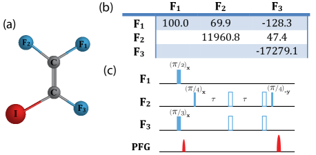
Figure 2: The molecular structure of trifluoroiodoethylene (a), and corresponding chemical shifts and J-coupling values(in Hz) (b), and the pulse sequence for the preparation of initial state (c). The open pulses are π𝜋\pi pulses and τ=1/(4J23)𝜏14subscript𝐽23\tau=1/(4J_{23}).

We have employed a model as shown in Fig. 1 for measuring TTJP nmr_elgi . The grouped gates represent the measurements in the rotated bases. The controlled gates shown can be either CNOT or anti-CNOT gate. We require both CNOT and anti-CNOT gate to perform the ‘ideal negative result measurement’ (INRM) procedure to measure the TTJP noninvasively, as proposed by Knee et.al. noninvasive . The idea behind the INRM procedure is as follows: consider a gate which interacts with the ancilla qubit only when the system qubit is in state |1ket1|{1}\rangle. By application of such a gate we can noninvasively obtain the probability of the measurement outcomes when the system was in |0ket0|{0}\rangle state. Similarly if we have a gate, which can interact with ancilla only if the system qubit is in |0ket0|{0}\rangle state then we can noninvasively obtain the probability of the measurement outcomes of the system state being in |1ket1|{1}\rangle. These criteria are fulfilled by the CNOT gate and the anti-CNOT gate respectively.

Circuit shown in Fig. 1 has two controlled gates for encoding the outcomes of first and second measurements on to the first and second ancilla qubits respectively. The third measurement need not be non-invasive since we are not concerned with the further time evolution of the system. A set of four experiments are to be performed, with following arrangement of first and second controlled gates for measurement of the TTJP: (i) CNOT; CNOT, (ii) anti-CNOT; CNOT, (iii) CNOT; anti-CNOT, and (iv) anti-CNOT; anti-CNOT.

The propagators U^i=eiσxωti/2subscript^𝑈𝑖superscript𝑒𝑖subscript𝜎𝑥𝜔subscript𝑡𝑖2\hat{U}_{i}=e^{-i\sigma_{x}\omega t_{i}/2} is realized by the cascade U^dsubscript^𝑈𝑑\mathbb{H}\hat{U}_{d}\mathbb{H}, where \mathbb{H} is the Hadamard gate, and the delay propagator U^d=eiσzωti/2subscript^𝑈𝑑superscript𝑒𝑖subscript𝜎𝑧𝜔subscript𝑡𝑖2\hat{U}_{d}=e^{-i\sigma_{z}\omega t_{i}/2} corresponds to the z-precession of the system qubit at ω=2π100𝜔2𝜋100\omega=2\pi 100 rad/s resonance off-set. The diagonal tomography was performed at the end to determine the probabilities nmr_elgi .

Refer to caption
Figure 3: Moussa Protocol for obtaining the 333-time correlated moments. One and two time moments can be calculated using the appropriate number of controlled gates.
Refer to caption
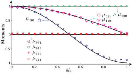
Figure 4: Moments obtained experimentally from Moussa Protocol. The symbols represent experimentally obtained values of the indicated moments with the solid lines showing the corresponding theoretical values.

The three qubits were provided by the three 19F nuclear spins of trifluoroiodoethylene dissolved in acetone-D6. The structure of the molecule is shown in Fig. 2(a) and the chemical shifts and the scalar coupling values (in Hz) in Fig. 2(b). The effective 19F spin-lattice (T2superscriptsubscriptabsent2{}_{2}^{*}) and spin-spin (T1) relaxation time constants were about 0.80.80.8s and 6.36.36.3 s respectively. The experiments were carried out at an ambient temperature of 290 K on a 500 MHz Bruker UltraShield NMR spectrometer. The first spin (F1) is used as the system qubit and, other spins (F2 and F3) as the ancilla qubits. Initialization involved preparing the state, 1ϵ8𝟙+ϵ{12𝟙S|0000|A}1italic-ϵ81italic-ϵtensor-product12subscript1𝑆ket00subscriptbra00𝐴\frac{1-\epsilon}{8}\mathbbm{1}+\epsilon\left\{\frac{1}{2}\mathbbm{1}_{S}\otimes|{00}\rangle\langle{00}|_{A}\right\} where ϵ105similar-toitalic-ϵsuperscript105\epsilon\sim 10^{-5} is the purity factor cory . The pulse sequence to prepare this state from the equilibrium state is shown in Fig. 2(c). All pulses were numerically optimized using the GRAPE technique Khaneja and had fidelities better than 0.9990.9990.999.

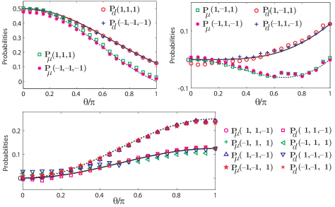
With our choice of measurement model (Fig. 1) we find a striking agreement with theoretical results on TTJP (III) . One might have also run the post measured state resulting after the first dashed block in Fig. 1 through an arbitrary CP map before the next step. However such post processing CP map would have affected the results. In other words, our measurement scheme provides an optimal procedure to preserve the state information, thus resulting in an excellent agreement of experimental results on TTJP with theoretical prediction (see Fig. 5).

For calculating the moments we utilize the Moussa protocol Moussa , which requires only two spins in our case. We utilize F1 as the system and F2 as the ancilla qubit. F3 was decoupled using π𝜋\pi pulses and the initialization involved preparing the state, 1ϵ8𝟙+ϵ{12𝟙S|++|A|00|}\frac{1-\epsilon}{8}\mathbbm{1}+\epsilon\left\{\frac{1}{2}\mathbbm{1}_{S}\otimes|{+}\rangle\langle{+}|_{A}\otimes|{0}\rangle\langle{0}|\right\}, which is obtained by applying the Hadamard gate to F2 after the pulse sequence shown in Fig. 2(c). The circuit for measuring moments by Moussa protocol is shown in Fig. 3 and it proceeds as follows,

ρ^|++|\displaystyle\hat{\rho}\otimes|{+}\rangle\langle{+}|
cX^1absentcsubscript^X1\displaystyle\downarrow\mathrm{c\hat{X}_{1}}
ρ^X^1|01|+X^1ρ^|10|+tensor-product^𝜌superscriptsubscript^X1ket0bra1limit-fromtensor-productsubscript^X1^𝜌ket1bra0\displaystyle\hat{\rho}\mathrm{\hat{X}_{1}}^{\dagger}\otimes|{0}\rangle\langle{1}|+\mathrm{\hat{X}_{1}}\hat{\rho}\otimes|{1}\rangle\langle{0}|+
ρ^|00|+X^1ρ^X^1|11|tensor-product^𝜌ket0bra0tensor-productsubscript^X1^𝜌superscriptsubscript^X1ket1bra1\displaystyle\hat{\rho}\otimes|{0}\rangle\langle{0}|+\mathrm{\hat{X}_{1}}\hat{\rho}\mathrm{\hat{X}_{1}}^{\dagger}\otimes|{1}\rangle\langle{1}|
cX^2absentcsubscript^X2\displaystyle\downarrow\mathrm{c\hat{X}_{2}}
ρ^X^1X^2|01|+X^2X^1ρ^|10|+tensor-product^𝜌superscriptsubscript^X1superscriptsubscript^X2ket0bra1limit-fromtensor-productsubscript^X2subscript^X1^𝜌ket1bra0\displaystyle\hat{\rho}\mathrm{\hat{X}_{1}}^{\dagger}\mathrm{\hat{X}_{2}}^{\dagger}\otimes|{0}\rangle\langle{1}|+\mathrm{\hat{X}_{2}}\mathrm{\hat{X}_{1}}\hat{\rho}\otimes|{1}\rangle\langle{0}|+
ρ^|00|+X^2X^1ρX^1X^2|11|tensor-product^𝜌ket0bra0tensor-productsubscript^X2subscript^X1𝜌superscriptsubscript^X1superscriptsubscript^X2ket1bra1\displaystyle\hat{\rho}\otimes|{0}\rangle\langle{0}|+\mathrm{\hat{X}_{2}}\mathrm{\hat{X}_{1}}\rho\mathrm{\hat{X}_{1}}^{\dagger}\mathrm{\hat{X}_{2}}^{\dagger}\otimes|{1}\rangle\langle{1}|
cX^3absentcsubscript^X3\displaystyle\downarrow\mathrm{c\hat{X}_{3}}
ρ^X^1X^2X^3|01|+X^3X^2X^1ρ^|10|+tensor-product^𝜌superscriptsubscript^X1superscriptsubscript^X2superscriptsubscript^X3ket0bra1limit-fromtensor-productsubscript^X3subscript^X2subscript^X1^𝜌ket1bra0\displaystyle\hat{\rho}\mathrm{\hat{X}_{1}}^{\dagger}\mathrm{\hat{X}_{2}}^{\dagger}\mathrm{\hat{X}_{3}}^{\dagger}\otimes|{0}\rangle\langle{1}|+\mathrm{\hat{X}_{3}}\mathrm{\hat{X}_{2}}\mathrm{\hat{X}_{1}}\hat{\rho}\otimes|{1}\rangle\langle{0}|+
ρ^|00|+X^3X^2X^1ρ^X^1X^2X^3|11|,tensor-product^𝜌ket0bra0tensor-productsubscript^X3subscript^X2subscript^X1^𝜌superscriptsubscript^X1superscriptsubscript^X2superscriptsubscript^X3ket1bra1\displaystyle\hat{\rho}\otimes|{0}\rangle\langle{0}|+\mathrm{\hat{X}_{3}}\mathrm{\hat{X}_{2}}\mathrm{\hat{X}_{1}}\hat{\rho}\mathrm{\hat{X}_{1}}^{\dagger}\mathrm{\hat{X}_{2}}^{\dagger}\mathrm{\hat{X}_{3}}^{\dagger}\otimes|{1}\rangle\langle{1}|,

where, cX^icsubscript^Xi\mathrm{c\hat{X}_{i}} represents the controlled gates and ρ^^𝜌\hat{\rho} is the initial state of the system. The state of the ancilla qubit (ρ^asubscript^𝜌𝑎\hat{\rho}_{a}) at the end of the circuit is given by,

ρ^asubscript^𝜌𝑎\displaystyle\hat{\rho}_{a} =\displaystyle= |01|Tr(ρ^X^1X^2X^3)+|10|Tr(X^3X^2X^1ρ^)ket0quantum-operator-product1limit-fromTr^𝜌superscriptsubscript^𝑋1superscriptsubscript^𝑋2superscriptsubscript^𝑋31bra0Trsubscript^𝑋3subscript^𝑋2subscript^𝑋1^𝜌\displaystyle|{0}\rangle\langle{1}|{\rm Tr}(\hat{\rho}\hat{X}_{1}^{\dagger}\hat{X}_{2}^{\dagger}\hat{X}_{3}^{\dagger})+|{1}\rangle\langle{0}|{\rm Tr}(\hat{X}_{3}\hat{X}_{2}\hat{X}_{1}\hat{\rho})
+|00|Tr(ρ^)+|11|Tr(X^3X^2X^1ρ^X^1X^2X^3).ket0quantum-operator-product0limit-fromTr^𝜌1bra1Trsubscript^𝑋3subscript^𝑋2subscript^𝑋1^𝜌superscriptsubscript^𝑋1superscriptsubscript^𝑋2superscriptsubscript^𝑋3\displaystyle+|{0}\rangle\langle{0}|{\rm Tr}(\hat{\rho})+|{1}\rangle\langle{1}|{\rm Tr}(\hat{X}_{3}\hat{X}_{2}\hat{X}_{1}\hat{\rho}\hat{X}_{1}^{\dagger}\hat{X}_{2}^{\dagger}\hat{X}_{3}^{\dagger}).

Moussa protocol was originally proposed for commutating observables, however, it can be easily extended to non-commutating observables. The NMR measurements correspond to the expectation values of spin angular momentum operators Ixsubscript𝐼𝑥I_{x} or Iysubscript𝐼𝑦I_{y}cavanagh . The measurement of the Ixsubscript𝐼𝑥I_{x} for ancilla qubit at the end of the circuit gives:

Tr[ρ^aIx]=Tr[X^3X^2X^1ρ^]/2+Tr[ρ^X^1X^2X^3]/2.Trdelimited-[]subscript^𝜌𝑎subscript𝐼𝑥Trdelimited-[]subscript^𝑋3subscript^𝑋2subscript^𝑋1^𝜌2Trdelimited-[]^𝜌superscriptsubscript^𝑋1superscriptsubscript^𝑋2superscriptsubscript^𝑋32{\rm Tr}[\hat{\rho}_{a}I_{x}]={\rm Tr}[\hat{X}_{3}\hat{X}_{2}\hat{X}_{1}\hat{\rho}]/2+{\rm Tr}[\hat{\rho}\hat{X}_{1}^{\dagger}\hat{X}_{2}^{\dagger}\hat{X}_{3}^{\dagger}]/2. (20)

If, X^1,X^2,X^3subscript^𝑋1subscript^𝑋2subscript^𝑋3\hat{X}_{1},\hat{X}_{2},\hat{X}_{3} commute, then the above expression gives Tr[ρ^X^1X^2X^3]Trdelimited-[]^𝜌subscript^𝑋1subscript^𝑋2subscript^𝑋3\mathrm{Tr}[\hat{\rho}\hat{X}_{1}\hat{X}_{2}\hat{X}_{3}]. In case of non-commuting hermitian observables, we also measure expectation value of Iysubscript𝐼𝑦I_{y}, which gives :

iTr[ρaIy]=Tr[X^3X^2X^1ρ^]/2Tr[ρ^X^1X^2X^3]/2.𝑖Trdelimited-[]subscript𝜌𝑎subscript𝐼𝑦Trdelimited-[]subscript^𝑋3subscript^𝑋2subscript^𝑋1^𝜌2Trdelimited-[]^𝜌superscriptsubscript^𝑋1superscriptsubscript^𝑋2superscriptsubscript^𝑋32i{\rm Tr}[\rho_{a}I_{y}]={\rm Tr}[\hat{X}_{3}\hat{X}_{2}\hat{X}_{1}\hat{\rho}]/2-{\rm Tr}[\hat{\rho}\hat{X}_{1}^{\dagger}\hat{X}_{2}^{\dagger}\hat{X}_{3}^{\dagger}]/2. (21)

From (20) and (21) we can calculate Tr[ρ^X^1X^2X^3]X^1X^2X^3Trdelimited-[]^𝜌subscript^𝑋1subscript^𝑋2subscript^𝑋3delimited-⟨⟩subscript^𝑋1subscript^𝑋2subscript^𝑋3\mathrm{Tr}[\hat{\rho}\hat{X}_{1}\hat{X}_{2}\hat{X}_{3}]\equiv\langle\hat{X}_{1}\hat{X}_{2}\hat{X}_{3}\rangle for the 333-measurement case. Hence, by using the different number of controlled gates in appropriate order we can calculate all the moments. The experimentally obtained moments are shown in Fig. 4.
Refer to caption
Figure 5: Three-time joint probabilities (TTJP): The solid curve represents the probabilities obtained directly and the dashed curve the probabilities obtained by inverting the moments. The symbols represents the experimental data.

These experimentally obtained moments are inverted according to Eq. (II) to calculate the TTJP and are plotted along with the directly obtained TTJP using circuit shown in Fig. 1 as symbols in Fig. 5. The theoretical values for TTJP from moments and the one directly obtained are plotted as solid and dashed lines respectively. The results agree with the predictions of Eqs. (III) and (III) that the TTJP obtained directly and the one obtained from the inversion of moments do not agree.

V Conclusion

In classical probability setting, statistical moments associated with dichotomic random variables determine the probabilities uniquely. When the same issue is explored in the quantum context – with random variables replaced by Hermitian observables (which are in general non-commuting) and the statistical outcomes of observables in sequential measurements are considered – it is shown that the joint probabilities do not agree with the ones inverted from the moments. This is explicitly illustrated by considering sequential measurements of a dynamical variable at three different times in the specific example of a spin-1/2 system. An experimental investigation based on NMR methods, where moments and the joint probabilities are extracted independently, demonstrates the moment indeterminacy of probabilities, concordant with theoretical observations.

The failure to revert joint probability distribution from its moments points towards its inherent incompatibility with the family of all marginals. In turn, the moment indeterminacy reveals the absence of a legitimate joint probability distribution compatible with the set of all marginal distributions – a common underpinning of various no-go theorems in the foundational aspects of quantum theory.

Acknowledgements

The authors are grateful to K. R. Koteswara Rao and Sudha for discussions. This work was partly supported by the DST project SR/S2/LOP-0017/2009.

References