A possible approach on optical analogues of gravitational attractors

Abstract

In this paper we report on the feasibility of light confinement in orbital geodesics on stationary, planar, and centro-symmetric refractive index mappings. Constrained to fabrication and [meta]material limitations, the refractive index, $n$, has been bounded to the range: $0.8\leq n\left(\vec{r}\right)\leq 3.5$. Mappings are obtained through the inverse problem to the light geodesics equations, considering trappings by generalized orbit conditions defined a priori. Our simulation results show that the above mentioned refractive index distributions trap light in an open orbit manifold, both perennial and temporal, in regards to initial conditions. Moreover, due to their characteristics, these mappings could be advantageous to optical computing and telecommunications, for example, providing an on-demand time delay or optical memories. Furthermore, beyond their practical applications to photonics, these mappings set forth an attractive realm to construct a panoply of celestial mechanics analogies and experiments in the laboratory.
Published at Optics Express 21, 8298–8310, 2013. DOI: 10.1364/OE.21.008298.

I Introduction

Einstein’s general relativity theory allows us to understand the dynamics of mass and massless particles as they travel through space-time. From it, we learn that matter and geometry are inextricably related; the latter transfigures the metric of space-time, and this alteration in turn modifies the geodesics, the paths of particles, resulting in a manifold of relativistic effects, v. gr. the apparent shift in the position of the stars due to the gravitational lensing effect, depicted in Fig. 1a, where photons traveling near a massive star are deflected from their otherwise straight path due to the curvature of space-time; or trapping in multifarious orbits around black holes with respect to the initial conditions and shape of the gravitational attractor Levin2008 ; Hloe2010 ; Muller2011 , see Figs. 1b and 1c.

Keeping in mind the previous illustrations, let us momentarily examine a more mundane experiment. Imagine a photon moving in a region of space filled with some monotonically increasing refractive index. What we observe as the photon moves in the medium is that its path describes a curve like the one depicted in Fig. 1d. If the gradient of the refractive index is tailored properly, it would be possible to build an optical analogy to gravitational bending (see Fig. 1a) for example. This leads us to wonder whether it is possible to fabricate an optical analogue to other sidereal geodesics by means of a differential control on the index of refraction.

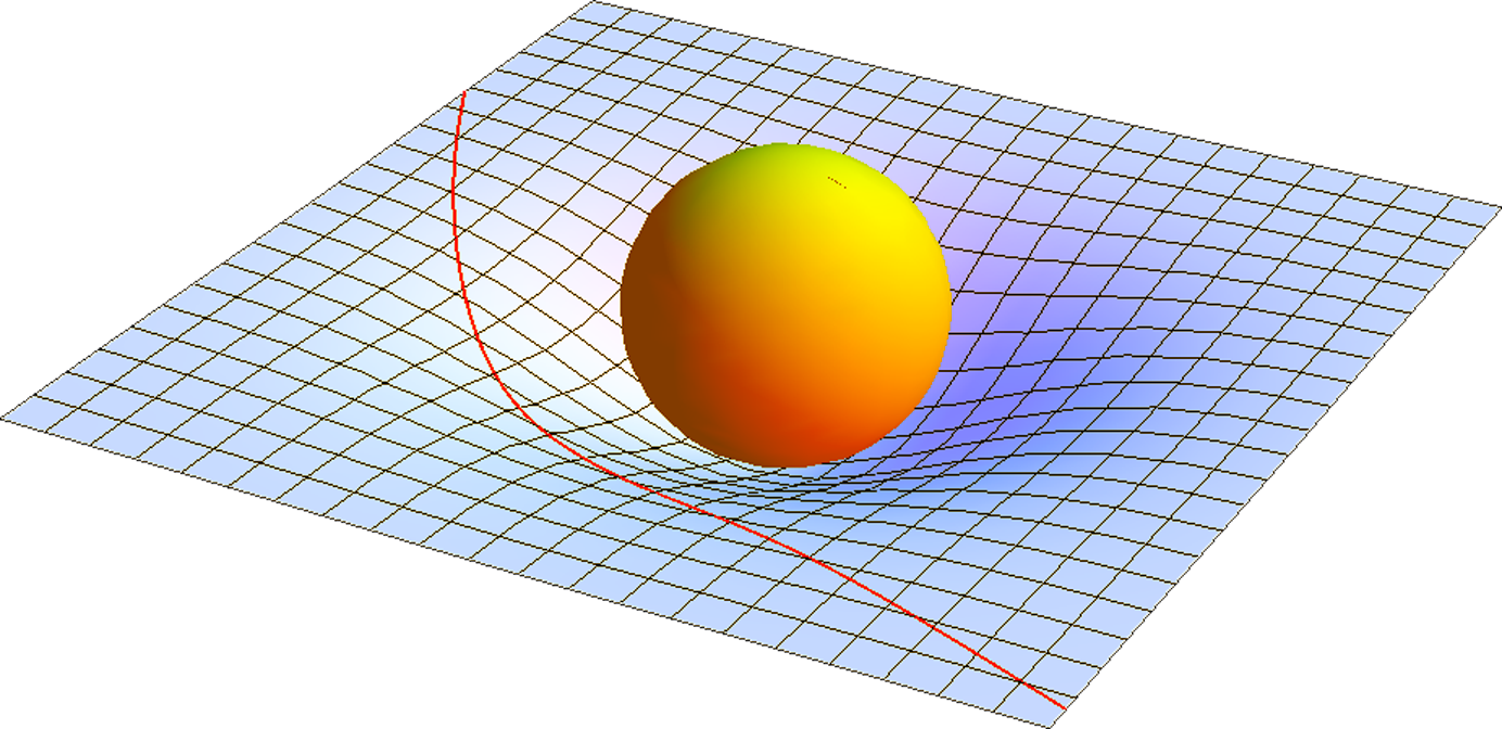
(a)  

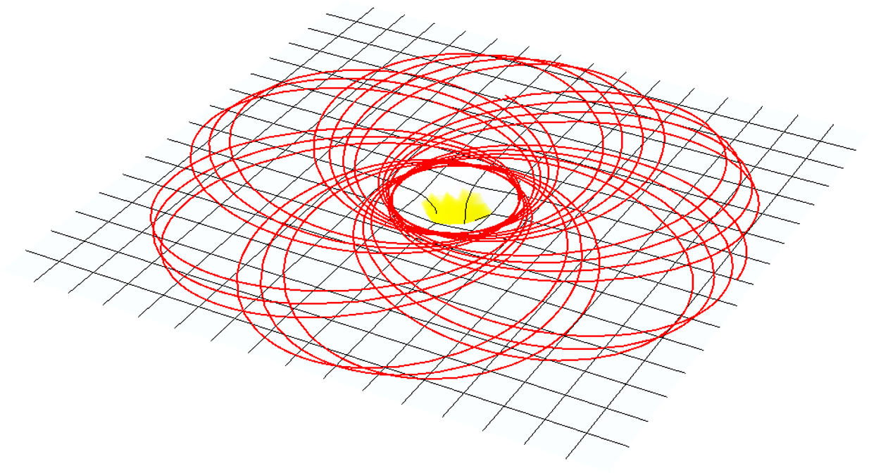
(b)  

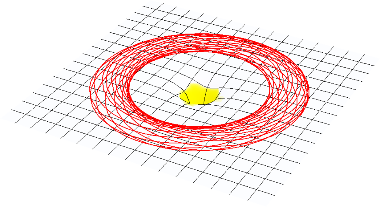
(c)  

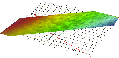
(d)  

Figure 1: Comparison of sidereal and laboratory frame geodesics for light beams in (a) the vicinity of a star, (b) and (c) spinning black hole at different initial conditions, and (d) the laboratory across an heterogeneous monotonic increasing refractive index medium.

The latter analogy reveals a connection between both examples, a weft where both realms [sidereal and laboratory] can be understood as manifestations of the same mathematical ground, albeit significantly different physics, differential geometry. Einstein’s general theory of relativity tells us that geometry and gravity are linked by means of the metric tensor of space-time; in optics the intricacy of the relation between geometry and the physical properties of materials (permittivity and permeability) has been evinced by miscellaneous methods, most based on differential geometry Leonhardt2008a ; Chen2010 ; Pendry2006 ; Schurig2006 .

These methods can be used to show that the optical example of differential light bending can be understood in terms of geometry, essentially by bending the space on which the light propagates, hence the metric is related to the electromagnetic tensors Leonhardt2008a ; Pendry2006 . This realization paved the way for the theoretical realization of optical cloaks, super-lenses, optical illusion devices and recently black-hole analogues in moving refractive index perturbations Pendry2006 ; Schurig2006 ; Leonhardt1999 ; Leonhardt2000 ; Brevik2001 ; Liu2009 ; Ergin2010 ; Lai2009 ; Kwon2009 .

Concerning trapping and light confinement in particular, different methods have been proposedHloe2010 ; Genov2009 ; Piwnicki2001 ; Cacciatori2010 . Of particular interest is Genov et al study, which presented an isotropic inhomogeneous refractive index mapping which was able to confine light mimicking a closed orbit around a black hole Genov2009 . As the authors noted, such mapping could be implemented on a dielectric photonic crystal, composed of air-gaps in Gallium-Arsenide.

In our work, we posit theoretical traps that provide an optical analogue to celestial mechanics to realize light confinement, trapping in a region of space, by means of two-dimensional stationary refractive index mappings, which could be implemented under current technological and photo-refractive [meta]materials, constraint to optical frequencies, which could be easily integrable on all-optical-chips Sanroman2012 ; Zakery2003 ; Kang2009 ; Sanroman2013 . The mathematical and physical background to make these effects possible could bring forth an exciting ground to test sidereal mechanics in the laboratory; and provide the key to enable a miscellany planar optical systems that are of great interest for diverse photonic applications, ranging from time delays, to temporal optical memories, or random resonators, to name a few; thence its significance.

II Deriving the model

We regard a model equation based in the paraxial approximation of non-linear electrodynamics, by looking into a medium where the index of refraction can be modulated in space and time by some smooth varying function $f$, e.g. in photo-refractive media index of refraction is a real valued function $f$ of the incident light intensity $I$; therefore $n(\vec{x})=f(I(\vec{x}))$, where $\vec{x}$ is the space-time quadrivector which corresponds to the coordinates $\{x^{0}:x^{1},x^{2},x^{3}\}$. In this representation $x^{0}$ corresponds to the time coordinate, and the rest to the usual three-dimensional space. In this context the photon’s path is governed by the geometry of the space the light is propagating on, which in general has the metric tensor $g_{ij}$, and the infinitesimal length element $ds^{2}=g_{ij}dx^{i}dx^{j}$. Therefore, if we parameterized the path followed by light with reference to the proper time $\tau$, i.e. $\vec{x}(\tau)$, we can analytically derive the path equations by means of Lagrange-Euler equations, whit a Lagrangian of the form:

$$L=\frac{1}{2}\left[g_{ij}\frac{\partial x^{i}}{\partial\tau}\frac{\partial x^{j}}{\partial\tau}\right],$$ (1)

where the derivatives are taken in respect to the affine parameter $\tau$, i.e. the proper time.

The physical description behind Eq. (1) is relevant to optics, as we set forth earlier in the introduction. If the metric were indeed related to the electromagnetic tensors, permittivity and permeability, then it could be possible to write the light-path in the paraxial approximation as a function of either the refractive index $n=f(x^{0},\vec{r})=\sqrt{\varepsilon(\vec{r},t)\mu(\vec{r},t)}$, or the metric $ds$. Hence, it could be possible to use Fermat’s principle, where Eq. (1) would take the role of an optical Lagrangian, i.e. the solution to the variational problem which states that given a refractive index $n(x^{0},\vec{r})$ the path light follows is given by the extrema of:

$$\delta\tau=\delta\int\limits_{x_{1}}^{x_{2}}ds=0,$$ (2)

where the integration is done between the arbitrary points $x_{1}^{j}$ to $x_{2}^{j}$, with $j=0,\ldots,3$, and $\delta$ indicates the functional maximization. Recursively, the solution to Eq. (2) is the Lagrange-Euler Eq. (1). Meanwhile, observe that in the integral of Eq. (2) the term $ds$ takes into account the metric by virtue of the covariant metric tensor $g_{ij}$ of the curved space:

$$ds=\sqrt{g_{ij}dx^{i}dx^{j}}.$$ (3)

Yet, we are still to determine the relation between the metric tensor $g_{ij}$ and the refractive index $n$. This can be achieved by means of conformal mappings, where it is possible to build the relation between the metric and the electromagnetic properties of a [meta]material Leonhardt2008a ; Chen2010 ; Pendry2006 . Specifically, if the line element of space-time  takes the form $ds^{2}=g_{00}dx^{0}dx^{0}-g_{ii}dx^{i}dx^{i}$, it is possible to map the curved space-time  to an isotropic, non-dispersive and non-absorbing medium as Leonhardt2008a ; Genov2009 :

$$n=\varepsilon=\mu=\sqrt{\frac{{-g}.g^{ij}}{g_{00}}},$$ (4)

where $g=\det{(g_{ij})}$. Furthermore if we consider Minkowski’s metric of special relativity, the tensor $g$ has the entries:

$$g=diag(g_{00},g_{11},g_{22},g_{33})=diag(1,-1,-1,-1),$$ (5)

then the refractive index $n=n(x^{0},\vec{r})$ can be found using Eq. (4). And consequently, the length element $ds$ of Eq. (2) can be written as:

$$ds^{2}=\frac{1}{n^{2}}dx^{0}dx^{0}-dx^{i}dx^{i},\quad i=1,2,3$$ (6)

II.1 Path equations and the inverse problem

Accordingly, from the Lagrange-Euler (1) we can derive the light-path, which in cylindrical coordinates takes the form:

$$\ddot{r} =r\dot{\phi}^{2}+\frac{\dot{t}^{2}\partial_{r}n}{n^{3}},$$ (7)

$$\ddot{\phi} =\frac{-2r\dot{r}\dot{\phi}+\frac{\dot{t}^{2}\partial_{\phi}n}{n^{3}}}{r^{2}},$$ (8)

$$\ddot{\phi} =\frac{\dot{t}^{2}\partial_{z}n}{n^{3}},$$ (9)

$$\ddot{t} =\frac{\dot{t}\left(\dot{t}\partial_{t}n+2\left(\dot{z}\partial_{z}n+\dot{\phi}\partial_{\phi}n+\dot{r}\partial_{r}n\right)\right)}{n},$$ (10)

where all derivatives marked by $\dot{\square}$ and $\ddot{\square}$ are with respect to the affine parameter $\tau$, e.g. $\dot{r}=\partial r/\partial\tau$. Equation (7) through Eq. (9) describe the parametrized path of a light beam traveling in a space-time with such geometry or equivalent refractive index.

We will describe light being trapped, when the geodesics are perpetually bounded to some region of space, for as long as the material properties remain unchanged. In this sense a light trapping geodesic is one where any of the following conditions arise:

1. $\dot{r},\dot{\phi}\rightarrow 0$,

2. $\dot{r}\rightarrow 0$ and $\phi_{min}\leq\phi\leq\phi_{max}$,

3. $\dot{\phi}\rightarrow 0$ and $r_{min}\leq r\leq r_{max}$,

4. $r_{min}\leq r\leq r_{max}$ and $\dot{\phi}_{min}\leq\dot{\phi}\leq\dot{\phi}_{max}$,

for all $\tau\geq\tau^{*}$; where $\tau^{*}$ marks the moment at which the initial conditions for trapping are met. The first condition is only possible if the refractive index $n$ goes to infinity, or if the refractive index co-moves with the wave Piwnicki2001 ; Cacciatori2010 . The other three cases can be realized in stationary refractive index Genov2009 ; Ni2011 . Thus, they can be imposed as general conditions to solve the inverse problem to Eq. (7) through Eq. (10).

The inverse problem begins by defining a set of a priori conditions that describes a generalized trapping scenario. If we impose premises 1 to 4, described earlier, the path equations reduce to new set of equations where the affine parameter is time itself; whence we can rework Eq. (7) through Eq. (10) into polar coordinates:

$$\ddot{r} =\frac{nr\dot{\phi}^{2}-2\dot{r}\dot{\phi}\partial_{\phi}n-\dot{r}^{2}\partial_{r}n+r^{2}\dot{\phi}^{2}\partial_{r}n}{n},$$ (11)

$$\ddot{\phi} =-\frac{2nr\dot{r}\dot{\phi}-\dot{r}^{2}\partial_{\phi}n+r^{2}\dot{\phi}^{2}\partial_{\phi}n+2r^{2}\dot{r}\dot{\phi}\partial_{r}n}{nr^{2}}.$$ (12)

Since we are interested in the general stationary case, we impose the fourth condition above, ensuing $0\leq\dot{r}\leq\dot{r}_{max}$ and $\dot{\phi}_{min}\leq\dot{\phi}\leq\dot{\phi}_{max}$, on Eq. (11) and Eq. (12), and find a non-singular refractive index distribution, $n(r,\phi)$, that satisfies them. Notice that we require the refractive index to be smoothly varying and $C^{2}$ continuous, i.e. $\nabla n\cdot\vec{e}^{i}\leq M$, where $M$ is a real valued number, and $\vec{e}^{i}$ a vector in a give direction in space-time. The general solution to this problem, however, is complex and a unique solution is not guaranteed Sanroman2012 ; 14 ; 31 .

The latter being said, the problem can be simplified further if we recall that a trapping orbit occurs when the radius $r$ is bounded to a region of space, i.e. $r_{min}\leq r\leq r_{max}$, for all $\phi$; whence $\dot{r}(r_{max})=\dot{t}(r_{min})=0$, and $r$ can be written in terms of the angle $\phi$ or the time $t$. Hence a natural solution to the inverse problem is an autonomous refractive index that varies with the radial variable, i.e. $n=n(r)$. This refractive index map resembles the centro-symmetric characteristics of gravitational fields, where, as pointed out independently by Genov and Ni Genov2009 ; Ni2011 , light would behave similarly to that traveling in curved space-time. Such distribution can be constrained to the conditions listed previously.

This result is significant in terms of fabrication where novel photo-refractive [metal]materials could be used. The refractive index in these composites can be modulated by the intensity of the change-inducing beam; which can be controlled by shaping its transversal profile Sanroman2012 ; Zakery2003 ; Kang2009 ; Sanroman2013 . Accordingly several families of refractive index distributions can be achieved, e.g. Gaussian, Laguerre, or Bessel, which are all centro-symmetrical.

II.2 System stability and dynamic equillibrium

Since the refractive index is a function of the radius, Eq. (11) and Eq. (12) can be rewritten in the form (13):

$$\ddot{x} =-h(x,\dot{x})-g(x),$$ (13)

$$\ddot{r} =\left(r^{2}\dot{\phi}^{2}-\dot{r}^{2}\right)\partial_{r}\ln{n}+r\dot{\phi}^{2},$$ (14)

$$\ddot{\phi} =-2\dot{r}\dot{\phi}\frac{n+r\partial_{r}n}{nr},$$ (15)

the system’s symmetry now allows us to integrate Eq. (15), hence:

$$\dot{\phi}=\frac{\ell}{\mu r^{2}},\quad\mu=n^{2},$$ (16)

where $\ell$ is a constant of integration. This equation is reminiscent of orbital mechanics, with the sole exception that $\mu$, the mass in celestial mechanics, varies with the radius. Substituting the latter result into Eq. (14), and rearranging yields:

$$\ddot{r}=\left(\frac{\ell^{2}}{n^{4}r^{4}}r^{2}-\dot{r}^{2}\right)\partial_{r}\ln n+\frac{\ell^{2}}{n^{4}r^{4}}r.$$ (17)

Equation (17) arrangement allows us to calculate the ratio of external energy supply, which is a measure of the equilibrium stability of the system Jordan2007 ; Verhulst1990 ; simplifying we get:

$$\mathcal{E}_{t}=\frac{\mathrm{d}\mathcal{E}}{\mathrm{d}t}=-\dot{r}h(r,\dot{r})=\dot{r}\left(\frac{\ell^{2}}{n^{4}r^{2}}-\dot{r}^{2}\right)\partial_{r}\ln n.$$ (18)

By virtue of Bertrand’s theorem Genov2009 ; Zarmi2002 , we know that $\dot{r}\neq 0$, for all time $t$; then from premises 3 and 4 it follows that $\dot{r}_{min}\leq\dot{r}\leq\dot{r}_{max}$, where $\dot{r}_{min}<0$; and from the definition of $n(r)$ as a monotonous decreasing function it follows that $\partial_{r}\ln n\leq 0$. Therefore, as the radius decreases, the radial velocity goes to its minimum and $\mathcal{E}_{t}\leq 0$, therefore the system approaches the equilibrium point and the amplitude of the path decreases. On the other hand, as the radius increases, the velocity tends to a maximum, and $\mathcal{E}_{t}\geq 0$, thus the system is driven away from the equilibrium point and the amplitude of the path increases. In Fig. 2 we show $\mathcal{E}_{t}$ for a Gaussian like refractive index described in section III.1. Observe that in the light confinement scenario we will see an oscillatory behavior in $\mathcal{E}_{t}$.

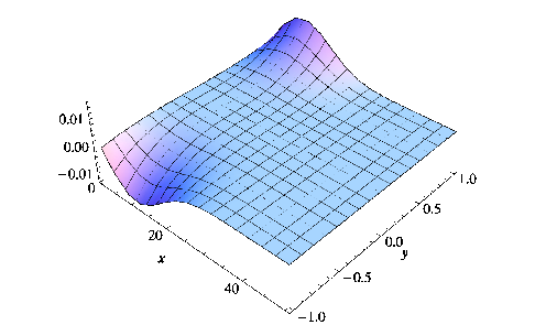
Figure 2: Ratio of external energy supply, $\mathcal{E}_{t}$, for a radial symmetric system, where $x=r$ and $y=\dot{r}$. Notice that there exists a $x_{c}$, critical radius, at wich for all phase space pairs $\{x,y|x\geq x_{c}\}$ $\mathcal{E}_{t}=0$, which implies that the light geodesics do not describe an orbital motion.

To conclude we study the stability of the orbits. by means of Lyapunov’s stability theory for the governing Eq. (17), and derive the constraints applicable to the refractive index mapping to attain stable orbital paths Genov2009 . First, let us rewrite Eq. (17) as:

$$\dot{r} =\varkappa,$$ (19)

$$\dot{\varkappa} =(r^{2}\beta^{2}-\varkappa^{2})\chi(r)+r\beta^{2},$$

with $\beta=\dot{\phi}$ and $\chi(r)=\partial_{r}\ln n$. Then, if we introduce small perturbations $r=r_{o}+\delta$ and $\varkappa=\varkappa_{o}+\epsilon$, expand $\chi(r)$ in a Taylor series around $r_{o}$, and drop all higher order terms for $\delta$ and $\epsilon$; we can rewrite Eq. (19) as a linear system of equations for the perturbation terms:

$$\left(\begin{matrix}\dot{\delta}\\ \dot{\epsilon}\end{matrix}\right)= \left(\begin{matrix}0&1\\ W&2V\end{matrix}\right)\left(\begin{matrix}\delta\\ \epsilon\end{matrix}\right),$$ (20)

$$V=-\varkappa_{o}\chi_{o}, W=2\chi_{o}\beta^{2}r_{o}+\chi^{\prime}_{o}(r_{o}^{2}\beta^{2}-\varkappa_{o}^{2}),$$

where $\chi_{o}$ and $\chi^{\prime}_{o}$ are the linear terms of the Taylor expansion of $\chi(r)$ around $r_{o}$. Ensuing the eigenvalues of the matrix above are given by:

$$\lambda_{1,2}=V\pm\sqrt{V^{2}+W}.$$ (21)

The geodesics will be stable if the real part of the eigenvalues of Eq. (20), $\Re\{\lambda_{1,2}\}$, are negative or equal to zero. Recall that $0\leq\beta\leq\lim_{r\to\infty}n(r)^{-1}$, and $\chi(r)\leq 0$; and therefore the condition for Lyapunov stability is reached if:

$${-\frac{\partial}{\partial r}\chi(r)}\bigg{|}_{r=r_{o}}\varkappa_{o}\leq 0,\qquad V^{2}+W\leq 0,$$ (22)

This constrained is met for all points $r$ near the stability point $r_{o}=0$, provided the radial velocity meets $\dot{r}_{o}\leq 0$. In general, since the refractive index is monotonous decrescent, the system will be Lyapunov stable at points where $\dot{r}\leq 0$, see, for example, the phase-space plots in Figs. 6b and 8b. In addition, it is interesting to analyze whether the system will be Lyapunov stable under the conditions necessary to sustain a circular orbit. In this case $\varkappa_{o}=0$, and $r_{o}=a$, constant, for all time $t$; consequently $V=0$, $W\leq 0$, and the second term in the equality (22) is imaginary, provided that $\chi(r)\leq 0$; thus resulting in $\Re\{\lambda_{1,2}\}=V=0$. These conditions, however, result in a different family of refractive indexes. In our study we focus on Gaussian-like refractive index distributions, feasible through photo-refraction, where $\varkappa\neq 0$, ergo the system will not describe closed circular orbits.

In summary, light confinement will occur as long as the conditions cited earlier apply. Under them the system will oscillate around the equilibrium point as depicted by the ratio of external energy supply. In the next section we will present the confinement geodesics resulting from these refractive index distributions. We will show that the geodesics in this system mimic those of a spinning black hole and other celestial objects, thus reproducing the paths of light traveling in curved space.

III Results and discussion

(a) $n_{a}=3.0,\quad n_{c}=0.8$

(b) $n_{a}=3.3,\quad n_{c}=0.5$

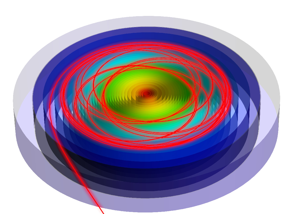
(c) $n_{a}=2.8,\quad n_{c}=1.0$

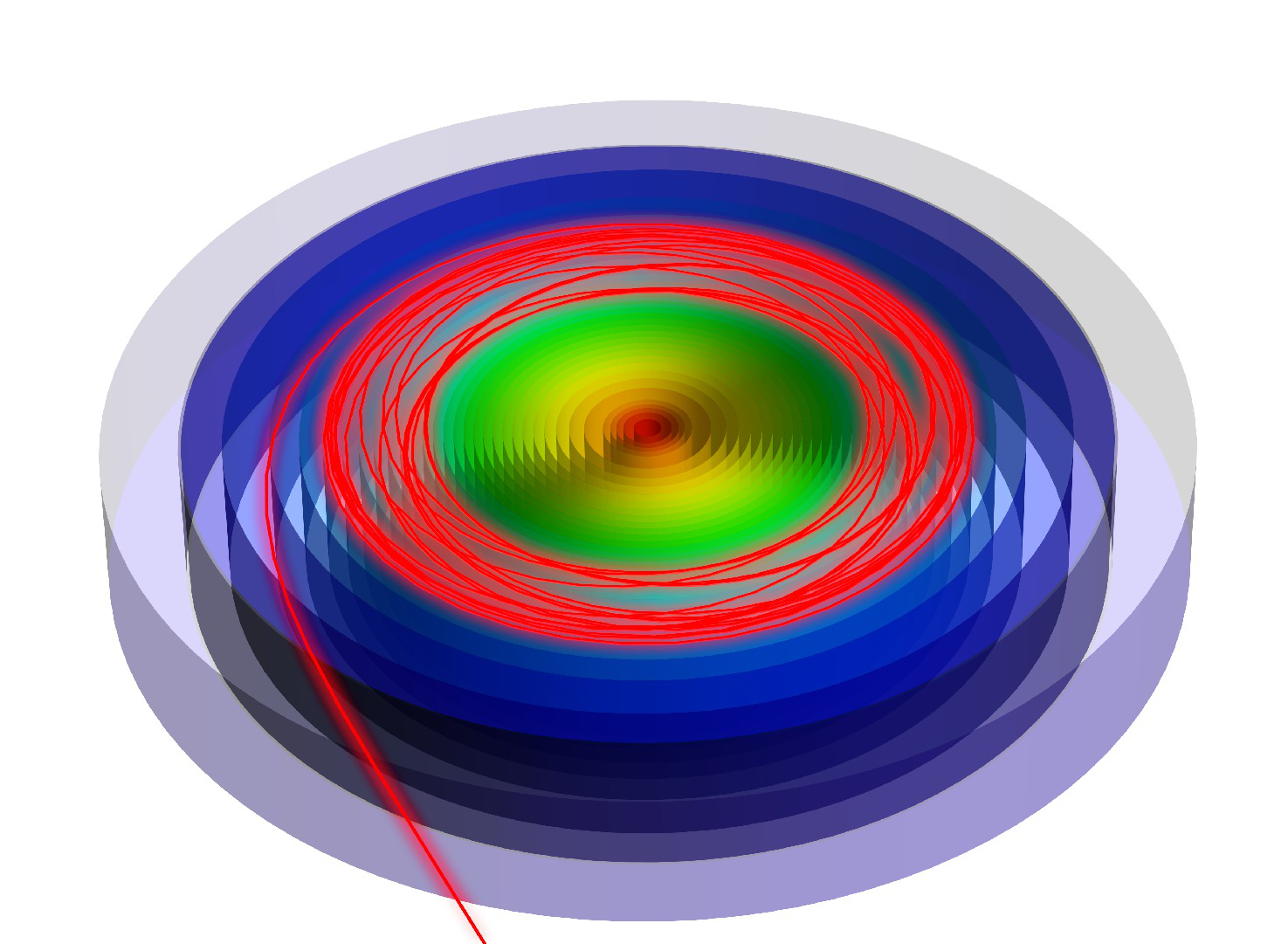
(d) $n_{a}=2.7,\quad n_{c}=1.1$

(e)

Figure 3: Light path dynamics for Gaussian refractive index shape for different $n_{a}$ and $n_{c}$. The maximum value of $n$ in all cases is $3.8$ at the center of the device. $\sigma$ is constant for all results. Notice the increment in the internal radius $r_{min}$ as $n_{c}$ increases, and the orbit width reduces.

In this section we explore three refractive index distributions based on Gaussian profiles. The first two mimic light trapped in the vicinity of a black hole, and the third case that of a particle moving in-between two planets.

III.1 Guassian distribution, single attractor

A Gaussian refractive index distribution has the form:

$$n=n_{a}e^{-r^{2}/\sigma^{2}}+n_{c}.$$ (23)

Then making it possible to constrain the maximum and minimum of the refractive index distribution to feasible values, e.g. $0.8n\leq 3.8$. Hence, given a range of values for the background and maximum refractive index, $n_{c}$ and $n_{a}$, respectively, we can evaluate different light confinement scenarios, see Fig. 3.

As discussed in the previous section the orbital paths are open, while their shape and stability depend significantly on the initial conditions, $n(r)$ and $\{r_{o},\dot{r}_{o},\phi_{o},\dot{\phi}_{o}\}$. As portrayed by Fig. 3 different initial conditions will result in new orbit manifolds with distinct characteristics, albeit maintaining a common morphology. As it can be seen from these figures the orbital paths are highly sensitive to the modifications in the refractive index and the initial conditions; a change in $\sim 0.5\%$ in $n_{c}$ alters the orbit, as seen from the plot of radii extrema in Fig. 4.

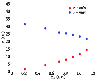
Figure 4: Inner and outer radius as a function of the background refractive index $n_{c}$. As it increases we observe that the outer radius diminishes, while the inner increases.

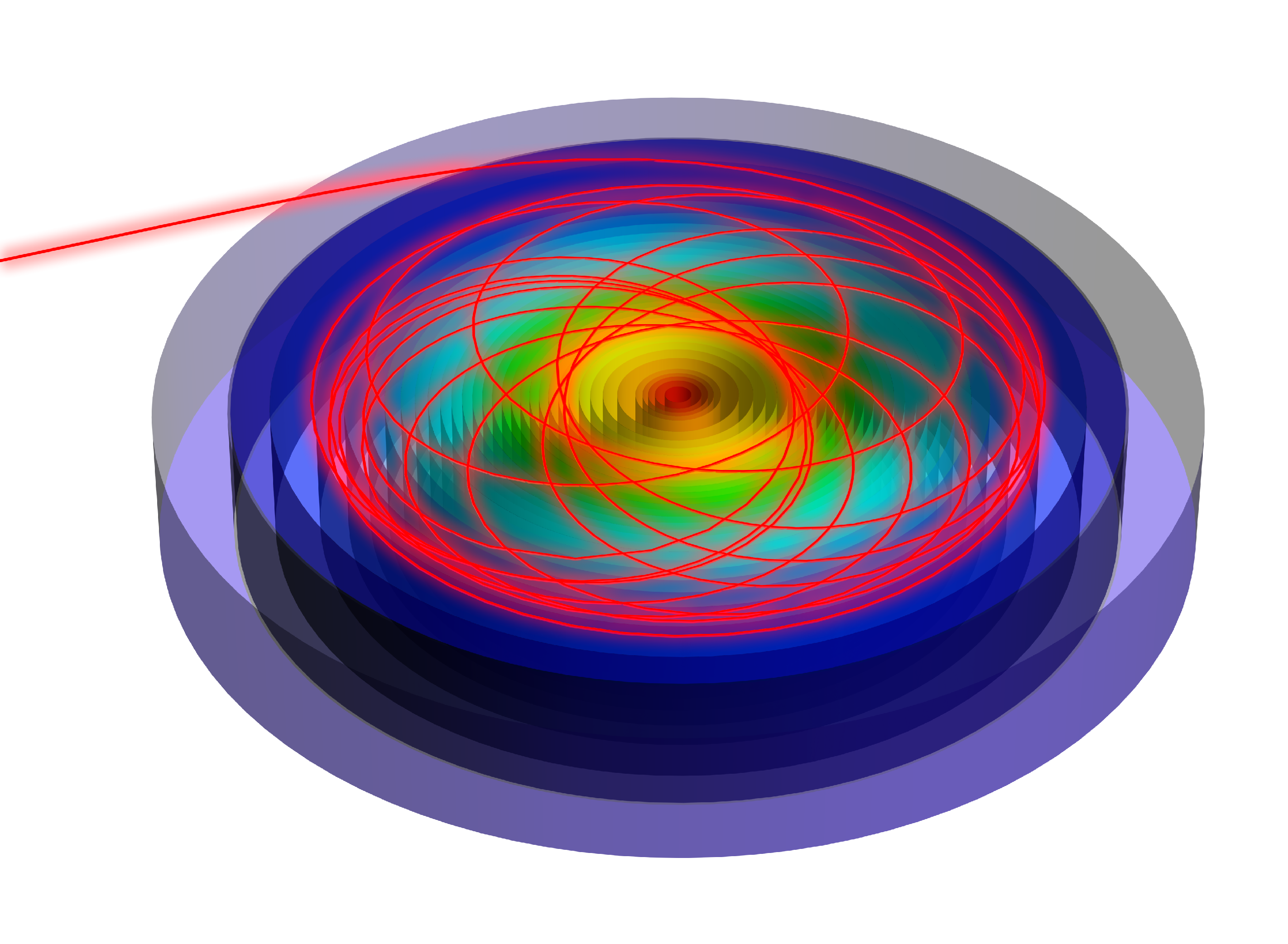
(a)

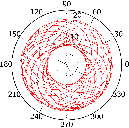
(b)

Figure 5: Confinement orbit for light traveling in a Gaussian attractor where $n_{a}=3.0$ and $n_{c}=0.8$. (a) Shows a schematic representation of the planar trapping device where the refractive index increases towards the center, where red indicates maximum refractive index $n=3.8$, and light blue $n=0.8$; (b) polar-2D path as calculated by the simulation routine.

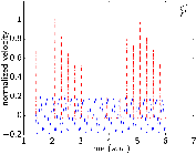
(a)

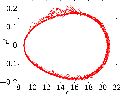
(b)

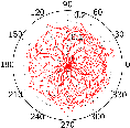
(c)

Figure 6: Phase space for Gaussian-like refractive index map with $n_{a}=3.0$, $n_{c}=0.8$. The plots show: (a) radial $\dot{r}$ and angular $\dot{\phi}$ velocities, (b) radial phase space, and (c) radial velocity as a function of the angle (c).

In Fig. 5 we show the 2D open orbit for a refractive index map where $n_{c}=0.8$ and $n_{a}=3.0$. As detailed in Fig. 6a, the radial velocity describes an oscillatory form, which indicates that the radius follows a similar motion, swinging between two extrema, as expected in a confine and open orbital motion. The latter can be observed in greater detail by analyzing the phase-space, plotted in Fig. 6b; notice that when the velocity $\dot{r}$ reaches zero the orbit radius $r$ reaches an extrema; for a closed single loop the amplitude of the velocity oscillation would be zero, and the phase space would become a horizontal line at $\dot{r}=0$. The behaviour of the angle versus the radial velocity, and consequently to the radius movement, is described by Fig. 6c, where the absolute value of the radial velocity is plotted against the angular position, which results in a periodic motion. Observe that in the limit at every angle there would be a time at which the radial velocity would be zero, which is typical of open orbits.

III.2 Mexican hat distribution

We study a variation on the Gaussian trap to understand the potential modifications on the trapping orbits when large modifications $\sim 20\%$ of the refractive index take place. The mathematical description of the mexican hat is:

$$n=(n_{a}-\frac{n_{d}r^{2}}{\sigma^{2}})e^{-r^{2}/\sigma^{2}}+n_{c}$$ (24)

Using the same conditions as in the previous analysis we set $n_{c}=0.8$, $n_{a}=3.0$, and set $n_{d}=0.2$. The results, shown in Figs. 7 and 8, display an orbit whose appearance resembles that of the regular Gaussian trap studied earlier. However, a closer look reveals that the trap confinement area is $\sim 2\%$ slimmer, and the oscillatory frequency of the radial and angular velocities, Fig. 8a, increases by $\sim 30\%$. Whereas the radial phase-space, Fig. 8b, shows a smaller eccentricity compared to its Gaussian counterpart, and the absolute value of the radial velocity versus the angle, Fig. 8c, describes the typical behaviour of an open orbit.

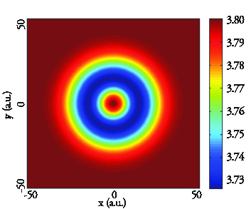
(a)

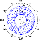
(b)

Figure 7: (a) Schematic of Mexican hat like refractive index map where $n_{a}=3.0$ and $n_{c}=0.8$ and depression is $n_{d}=0.2$; (b) depicts the resulting trapped orbit in polar coordinates as calculated by the simulation routine.

These variations in the trapping conditions could potentially be used to differentiate trapping in transient optical memories to allocated binary data.

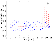
(a)

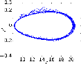
(b)

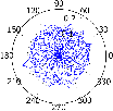
(c)

Figure 8: Phase-space for a mexican hat refractive index map with$n_{a}=3.0$, $n_{c}=0.8$. The plots show: (a) radial $\dot{r}$ and angular $\dot{\phi}$ velocities, (b) radial phase space, and (c) radial velocity as a function of the angle (c).

III.3 Double attractors

Interested in observing phenomenologically trapping in a binary system we evinced a planar refractive index map resulting from the superposition of two Gaussian functions,

$$n=n_{a}(e^{-(r-r_{off1})^{2}/\sigma^{2}}+e^{-(r-r_{off2})^{2}/\sigma^{2}})+n_{c}.$$ (25)

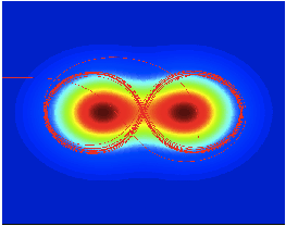
(a) $n_{a}=2.7,\quad n_{c}=1.1$

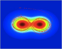
(b) $n_{a}=2.9,\quad n_{c}=.9$

Figure 9: Geodesics for light in a binary system. Observe that trapping also occurs for certain initial conditions at specific background and maximum refractive index.

The resulting orbits are shown in Fig. 9. A binary system, however, presents a relatively higher sensitivity to modifications in the refractive index, where a distortion of $\Delta n>0.03$ modifies the trapping orbits, in some cases releasing the light beam.Yet, it is possible to confine the light beam to an orbit which mimics the behaviour of Newton’s three body problem, where, as expected, small perturbations result in sundry possible solutions to the path equation, i.e. chaos.

III.4 The space-time equations, trapping

Briefly, we show that the same Gaussian solution explored in section III.1 fulfills the trapping conditions in the full eikonal space-time, Eq. (7) through Eq. (9). The results are shown in Fig. 10.

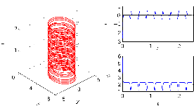
Figure 10: Phase space of the trapping orbit for $n_{a}=3.0$, $n_{c}=0.8$. The plots show: (a) radial $\dot{r}$ and angular $\dot{\phi}$ velocities, (b) radial phase space, and (c) radial velocity as a function of the angle.

In this case we observe a similar behaviour to that of the Gaussian trap in the stationary approximation, the difference in the amplitude values is due to normalization. An oscillatory behaviour in the radius and angular velocities is described in Figs. 10(b) and 10(c); as it would be expected from a centro-symmetrical refractive index mapping.

III.5 Material realization

Recent advancement in photo-refractive materials Sanroman2012 ; Zakery2003 ; Kang2009 ; Sanroman2013 could enable the construction of the light confinement devices discussed. For example, a prototype Gaussian trap could be fabricated by stacking different photo-refractive [meta]materials like $As_{x}S_{1-x}$ in multiple layers. Recalling that in photo-refraction the optical properties of the material, permeability and permittivity, change as a function of the light intensity, allowing the fabrication of a continuously varying refractive index as the one required by a centro-symmetrical attractors. Moreover, since photo-refractivity is elastic, i.e. reversible, it allows one to modify the refractive index of the layers combined in time, thence enabling or disabling the trap at will.

IV Conclusions

We have demonstrated that, under the paraxial description of light in heterogeneous media, it is possible to use centro-symmetrical refractive index distributions as attractors for light, which are able to perform light trapping or confinement in open orbits. These mappings are bound within fabrication constrains, and due to the paraxial approximation they are several times larger than the mean beam width and wavelength, $\sim 50$ times larger. The proposed mappings have potential applications to transient optical memories, delays, concentrators, random cavities, and beam stirrers, to cite a few; which could enable the next generation of photonic integrated circuits, PICs, processors and computation systems. Due to their sensitivity to the change in the refractive index these devices could be employed as a sensor platform. Furthermore, since they are drawn in close analogy to celestial phenomena they could be used as laboratory setups to test a large variety of effects in celestial mechanics.

References

- [1] J. Levin and G. Perez-Giz, “A periodic table for black hole orbits,” Phys. Rev. D77, 103005 (2008).
- [2] F. T. Hioe, and D. Kuebel, “Characterizing planetary orbits and trajectories of light in the Schwarzchild metric,” Phys. Rev. D81, 084017 (2010).
- [3] T. Müller, and J. Frauendiener, “Studying null and time-like geodesics in the classroom,” Eur. J. Phys. 32, 747–759 (2011).
- [4] U. Leonhardt and T. G. Philbin, “Transformation optics and the geometry of light,” in Progress in Optics 53, 69–153, E. Wolf, ed. (Elsevier, 2008).
- [5] H. Chen, C. T. Chan, and P. Sheng, “Transformation optics and metamaterials,” Nat. Mater. 9, 387–396 (2010).
- [6] J. B. Pendry, D. Schurig, and D. R. Smith, “Controlling electromagnetic fields,” Science 312, 1780–1782, 2006.
- [7] D. Schurig, J. B. Pendry, and D. R. Smith, “Calculation of material properties and ray tracing in transformation media,” Optics Express 14, 9794–9894 (2006).
- [8] U. Leonhardt and Piwnicki, “Optics of non-uniformly moving media,” Phys. Rev. A60, 4301–4312 (1999).
- [9] U. Leonhardt and Piwnicki, “Relativistic effects of light in moving media with extremely low group velocity,” Phys. Rev. Lett. 84, 822–825 (2000).
- [10] I. Brevik and G. Halnes, “Light rays at optical black holes in moving media,” Phys. Rev. D65, 024005 (2001).
- [11] R. Liu, C. Ji, J. J. Mock, J. Y. Chin, T. J. Cui, and D. R. Smith, “Broadband ground-plane cloak,” Science 323, 366–369 (2009).
- [12] T. Ergin, N. Stenger, Brenner, J. B. Pendry, and M. Wegener, “Three-dimensional invisibility cloak at optical wavelengths,” Science 328, 337–339 (2010).
- [13] Y. Lai, J. Ng, H. Chen, D. Han, J. Xiao, Z.-Q. Zhang, and C. Chan, “Illusion optics: the optical transformation of an object into another object,” Phys. Rev. Lett. 102, 253902 (2009).
- [14] D.-H. Kwon and D. H. Werner, “Flat focusing lens designs having minimized reflection based on coordinate transformation techniques,” Optics Express 17, 7807–7817 (2009).
- [15] D. Genov, S. Zhang, and X. Zhang, “Mimicking celestial mechanics in metamaterials,” Nat. Phys. 5, 687–692 (2009).
- [16] Piwnicki and U. Leonhardt, “Optics of moving media,” App. Phys. B 72, 51–59 (2001).
- [17] S. L. Cacciatori, F. Belgiorno, V. Gorini, G. Ortenzi, L. Rizzi, V. G. Sala, and D. Faccio, “Spacetime geometries and light trapping in travelling refractive index perturbations,” New J. Phys. 12, 095021 (2010).
- [18] D. P. San-Román-Alerigi, T. K. Ng, M. Alsunaidi, Y. Zhang, and B. S. Ooi, “Generation of -Bessel-Gauss beam by an heterogeneous refractive index map,” J. Opt. Soc. A 29, 1252–1258 (2012).
- [19] A. Zakery, “Optical properties and applications of chalcogenide glasses: a review,” J. Non-Crystaline Solids 330, 1–12 (2003).
- [20] S. B. Kang, M. H. Kwak, B. J. Park, S. K., H. C. Ryu, D. C. Chung, S. Y. Jeong, D. W. Kang, S. K. Choi, M. C. Paek, E. J. Cha, and K. Y. Kang, “Optical and dielectric properties of chalcogenide glasses at terahertz frequencies,” ETRI J. 31, 667–674 (2009).
- [21] D. P. San-Román-Alerigi, D. H. Anjum, Y. Zhang, X. Yang, A. B. Slimane, T. K. Ng, M. N. Hedhili, M. Alsunaidi, and B. S. Ooi, “Electron irradiation induced reduction of the permittivity of chalcogenide glass (As2S3) thin fim,” J. App. Phys. 113, 044116 (2013).
- [22] X. Ni and Y.-C. Lai, “Transient chaos in optical metamaterials,” Chaos 21, 033116 (2011).
- [23] B. Gangand and L. Peijun, “Inverse medium scattering problems for electromagnetic waves,” J. App. Math. 65, 2049–2066 (2005).
- [24] M. Piana, “On uniqueness for an isotropic inhomogeneous inverse scattering problems,” Inv. Problems 14, 1565–1579 (1998).
- [25] D. W. Jordan, and P. Smith, Nonlinear ordinary differential equations (Oxford University Press, 2007).
- [26] F. Verhulst, Nonlinear differential equations and dynamical systems (Springer Verlag, 1990).
- [27] Y. Zarmi, “The Bertrand theorem revisited,” Am. J. Phys 70, 446–449 (2002).