The EGNoG Survey: Molecular Gas in Intermediate-Redshift Star-Forming Galaxies

Abstract

We present the Evolution of molecular Gas in Normal Galaxies (EGNoG) survey, an observational study of molecular gas in 31 star-forming galaxies from $z=0.05$ to $z=0.5$, with stellar masses of $(4-30)\times 10^{10}$ M_⊙ and star formation rates of $4-100$ M_⊙ yr^-1. This survey probes a relatively un-observed redshift range in which the molecular gas content of galaxies is expected to have evolved significantly. To trace the molecular gas in the EGNoG galaxies, we observe the CO($J=1\rightarrow 0$) and CO($J=3\rightarrow 2$) rotational lines using the Combined Array for Research in Millimeter-wave Astronomy (CARMA). We detect 24 of 31 galaxies and present resolved maps of 10 galaxies in the lower redshift portion of the survey. We use a bimodal prescription for the CO to molecular gas conversion factor, based on specific star formation rate, and compare the EGNoG galaxies to a large sample of galaxies assembled from the literature. We find an average molecular gas depletion time of $0.76\pm 0.54$ Gyr for normal galaxies and $0.06\pm 0.04$ Gyr for starburst galaxies. We calculate an average molecular gas fraction of 7-20% at the intermediate redshifts probed by the EGNoG survey. By expressing the molecular gas fraction in terms of the specific star formation rate and molecular gas depletion time (using typical values), we also calculate the expected evolution of the molecular gas fraction with redshift. The predicted behavior agrees well with the significant evolution observed from $z\sim 2.5$ to today.

1. Introduction

In the past decade, molecular gas observations have begun probing the high redshift universe in a systematic way using increasingly powerful millimeter instruments. The picture that is emerging at redshifts $1-2$ is similar in some respects to what we see in the local universe. Sub-mm galaxies (SMGs) are observed to be undergoing extreme starbursts as a result of major mergers (e.g. Tacconi et al., 2008; Engel et al., 2010), equivalent to local ultra-luminous infrared galaxies (ULIRGs) (e.g. Sanders et al., 1986; Solomon et al., 1997; Downes & Solomon, 1998). Normal star-forming galaxies (SFGs) at high redshifts, akin to local spirals, are becoming accessible as well. Recent works (Tacconi et al., 2010; Daddi et al., 2010) suggest that $z\sim 1-2$ star-forming galaxies (with star formation rates (SFRs) of $\approx 50-200$ M_⊙ yr^-1) are scaled up versions of local spirals, forming stars in a steady mode (not triggered by interaction), despite hosting star formation rates at the level of typical local starburst systems like luminous infrared galaxies (LIRGs) and ULIRGS.

While galaxies classified as LIRGs or ULIRGs (by their infrared luminosities only) have typically been associated with starbursting and merging systems by analogy to galaxies in the local universe, it is becoming clear that this connection does not hold at high redshifts. Morphological studies find that while 50% of local LIRGs show evidence of major mergers (Wang et al., 2006), that fraction appears to decrease toward high redshifts: Bell et al. (2005) find that more than half of intensely star-forming galaxies at $z\approx 0.7$ have spiral morphologies and fewer than 30% show evidence of strong interaction. Further, the typical star formation rate of SFGs increases toward higher redshift. SFGs have been observed to obey a tight relation between stellar mass and star formation rate out to $z\sim 4$ (e.g. Brinchmann et al., 2004; Noeske et al., 2007; Elbaz et al., 2007; Daddi et al., 2007; Pannella et al., 2009; Daddi et al., 2009; Magdis et al., 2010). This ‘main sequence’ of SFGs evolves with redshift, shifting to higher star formation rates at higher redshifts.

The increase in the star formation rate is mirrored in the molecular gas fraction ($f_{\mathrm{mgas}}\equiv M_{\mathrm{mgas}}/(M_{*}+M_{\mathrm{mgas}}$), where $M_{\mathrm{mgas}}$ is the molecular gas mass (including He) and $M_{*}$ is the stellar mass) of these systems. While studies of local spirals (e.g. FCRAO survey, Young et al. 1995; BIMA SONG, Regan et al. 2001, Helfer et al. 2003; HERACLES, Leroy et al. 2009) find average molecular gas fractions of $\sim$5%, observations of high redshift SFGs suggest molecular gas fractions of 20-80%, an order of magnitude higher than local spirals. Unfortunately, the past 8 Gyr of the evolution of $f_{\mathrm{mgas}}$ remains relatively unprobed, with only one study of normal SFGs between $z=1$ and $z=0.05$ (Geach et al., 2011, at $z=0.4$).

Redshift	Redshift	Sample	Parent	M∗ Range	SFR Range	Observed	$\nu_{\mathrm{obs}}$	CARMA
Bin	Range	Size	Sample	(M⊙)	(M⊙ yr-1)	Transition	(GHz)	Configuration
A	0.05 - 0.10	13	SDSS	(4.0 - 16)$\times 10^{10}$	3.4 - 41	CO($J=1\rightarrow 0$)	107	C
B	0.16 - 0.20	10	SDSS	(6.3 - 32)$\times 10^{10}$	47 - 106	CO($J=1\rightarrow 0$)	98	D, some C
C	0.28 - 0.32	4	SDSS	(16 - 32)$\times 10^{10}$	39 - 65	CO($J=1\rightarrow 0$)	88	D
						CO($J=3\rightarrow 2$)	266	D, E
D	0.47 - 0.53	4	zCOSMOS	(4.0 - 5.5)$\times 10^{10}$	62 - 74	CO($J=3\rightarrow 2$)	230	D, E

Table 1Summary of the EGNoG survey.

To fill in this observational gap in redshift, we have carried out the Evolution of molecular Gas in Normal Galaxies (EGNoG) survey, a key project at the Combined Array for Research in Millimeter-wave Astronomy (CARMA). The EGNoG survey uses rotational transitions of the carbon monoxide (CO) molecule to trace the molecular gas content of 31 star-forming galaxies from $z=0.05$ to 0.5 (the CO($J=1\rightarrow 0$) line for galaxies at $z=0-0.3$ and the CO($J=3\rightarrow 2$) line for galaxies at $z=0.3-0.5$). The survey includes four galaxies at $z\approx 0.3$ (the gas excitation sample) observed in both the CO($J=1\rightarrow 0$) and CO($J=3\rightarrow 2$) lines, more than doubling the number of normal SFGs at $z>0.1$ in which CO line ratios have been measured. The results from the gas excitation sample are presented separately, in Bauermeister et al. (2013).

In this paper, we present the data for the entire EGNoG sample and use these data to constrain the evolution of the molecular gas fraction in galaxies at intermediate redshift. The paper is organized as follows. In Section 2 we describe the selection of the EGNoG survey galaxies and the properties of the sample. In Section 3 we describe the observations and data reduction (see Appedix B for a detailed description of the data reduction and Appendix C for polarization measurements of calibrators 0854+201 and 1058+015). We present the CO maps, total CO luminosities, and derived molecular gas masses in Section 4 and discuss the morphologies of the low-redshift portion of the sample as well as the non-detections of the high-redshift portion. In Section 5, we present a compilation of data from the literature and analyze the behavior of the molecular gas depletion time and molecular gas fraction in starburst and normal galaxies at low and high redshift. We provide some concluding remarks in Section 6.

Throughout this work, we use a $\Lambda$CDM cosmology with (h, $\Omega_{\mathrm{M}}$, $\Omega_{\Lambda}$) = (0.7, 0.3, 0.7). We use the following terms for star-forming galaxies at low and high redshift:

• Star-forming galaxy refers to any galaxy which is actively forming stars. Quantitatively, these galaxies lie on or above the main sequence of star-forming galaxies. This term encompasses both normal star-forming and starburst galaxies.

• Normal star-forming galaxy or SFG refers to star-forming galaxies that lie on the main sequence (within some scatter). While the acronym SFG stands for star-forming galaxy, we use it (in keeping with other authors) to refer to main sequence galaxies only, which comprise the bulk of the star-forming galaxy population.

• Starburst galaxy refers to a galaxy undergoing a period of enhanced star formation. We give a quantitative definition in Section 2.1.

• LIRG, ULIRG (luminous lnfrared galaxy, ultra-luminous lnfrared galaxy) denotes a galaxy with a total infrared luminosity between $10^{11}$ and $10^{12}$ L_⊙ (LIRG) or $>10^{12}$ L_⊙ (ULIRG). Local LIRGs and ULIRGs tend to be starbursts, but at high-redshift, normal star-forming galaxies would be classified as LIRGs or ULIRGs based on their infrared luminosities alone.

• SMG (sub-mm galaxy) refers to the population of galaxies at $z\gtrsim 1$ which have 850-$\mu$m fluxes $\gtrsim 4$ mJy. SMGs tend to be starbursts (often as a result of a merger, akin to local ULIRGs).

2. The EGNoG Sample

Utilizing the CO($J=1\rightarrow 0$) and CO($J=3\rightarrow 2$) in the 3 mm and 1 mm bands of CARMA, it is possible to achieve continuous redshift coverage from $z=0$ to $z\sim 0.5$. The EGNoG survey observed 31 galaxies spanning the accessible redshift range in 4 redshift bins, A-D. The redshift range, sample size, parent sample and range of M_∗ and SFR are given for each redshift bin in Table 1.

EGNoG	SDSS					SFR	sSFR
Name	Identification	RA	Dec	$z$	$\log(M_{*}/M_{\odot})$	(M⊙ yr-1)	(Gyr-1)
A1a	SDSS J234311.26+000524.3	23:43:11.257	+00:05:24.319	$0.096941\pm 0.000007$	$10.74^{+0.10}_{-0.09}$	$30.0^{+10.5}_{-8.1}$	0.54
A2	SDSS J231332.46+133845.3	23:13:32.468	+13:38:45.301	$0.081196\pm 0.000008$	$10.99^{+0.10}_{-0.10}$	$28.4^{+5.9}_{-5.2}$	0.29
A3	SDSS J233455.23+141731.0	23:34:55.239	+14:17:31.093	$0.062168\pm 0.000010$	$11.03^{+0.10}_{-0.09}$	$21.5^{+9.0}_{-6.4}$	0.20
A4	SDSS J085504.16+525248.4	08:55:04.171	+52:52:48.320	$0.089592\pm 0.000028$	$10.92^{+0.06}_{-0.10}$	$49.9^{+5.9}_{-4.6}$	0.60
A5	SDSS J085307.26+121900.8	08:53:07.258	+12:19:00.827	$0.080978\pm 0.000011$	$11.01^{+0.13}_{-0.11}$	$42.3^{+6.2}_{-6.3}$	0.42
A6	SDSS J084549.66+573239.3	08:45:49.662	+57:32:39.329	$0.085259\pm 0.000005$	$10.80^{+0.01}_{-0.01}$	$35.4^{+26.5}_{-9.0}$	0.56
A7	SDSS J211527.81-081234.4	21:15:27.817	-08:12:34.441	$0.090469\pm 0.000006$	$10.86^{+0.10}_{-0.09}$	$40.9^{+12.1}_{-8.7}$	0.57
A8	SDSS J135751.77+140527.3	13:57:51.775	+14:05:27.317	$0.099188\pm 0.000027$	$11.21^{+0.11}_{-0.10}$	$7.5^{+5.6}_{-2.8}$	0.05
A9	SDSS J105733.59+195154.2	10:57:33.589	+19:51:54.274	$0.077338\pm 0.000007$	$10.55^{+0.10}_{-0.09}$	$3.7^{+1.8}_{-1.1}$	0.10
A10	SDSS J141601.21+183434.1	14:16:01.216	+18:34:34.171	$0.055121\pm 0.000008$	$10.75^{+0.09}_{-0.09}$	$5.1^{+2.2}_{-1.4}$	0.09
A11	SDSS J100559.89+110919.6	10:05:59.890	+11:09:19.688	$0.076055\pm 0.000006$	$10.72^{+0.09}_{-0.08}$	$8.9^{+5.0}_{-2.4}$	0.17
A12	SDSS J111150.65+281147.7	11:11:50.654	+28:11:47.767	$0.098171\pm 0.000012$	$10.55^{+0.11}_{-0.09}$	$3.4^{+6.1}_{-1.9}$	0.10
A13	SDSS J221938.11+134213.9	22:19:38.115	+13:42:13.890	$0.083503\pm 0.000012$	$11.06^{+0.11}_{-0.10}$	$11.7^{+12.8}_{-5.8}$	0.10
B1	SDSS J223528.63+135812.6	22:35:28.638	+13:58:12.619	$0.183193\pm 0.000017$	$11.43^{+0.12}_{-0.13}$	$88.2^{+129.9}_{-50.5}$	0.33
B2	SDSS J002353.97+155947.8	00:23:53.973	+15:59:47.757	$0.191773\pm 0.000020$	$11.29^{+0.12}_{-0.11}$	$54.6^{+30.1}_{-22.5}$	0.28
B3	SDSS J100518.63+052544.2	10:05:18.640	+05:25:44.225	$0.165737\pm 0.000012$	$10.79^{+0.09}_{-0.09}$	$47.1^{+55.9}_{-23.3}$	0.76
B4a	SDSS J105527.18+064015.0	10:55:27.188	+06:40:15.025	$0.173078\pm 0.000013$	$11.02^{+0.11}_{-0.10}$	$49.7^{+82.8}_{-28.7}$	0.47
B5	SDSS J115744.35+120750.8	11:57:44.348	+12:07:50.792	$0.182661\pm 0.000010$	$11.24^{+0.10}_{-0.09}$	$51.1^{+19.3}_{-14.5}$	0.29
B6	SDSS J124252.54+130944.2	12:42:52.548	+13:09:44.215	$0.174661\pm 0.000013$	$10.83^{+0.23}_{-0.12}$	$59.2^{+15.9}_{-9.5}$	0.87
B7	SDSS J091426.24+102409.6	09:14:26.239	+10:24:09.649	$0.176180\pm 0.000018$	$11.45^{+0.10}_{-0.10}$	$61.5^{+83.6}_{-36.0}$	0.22
B8	SDSS J114649.18+243647.7	11:46:49.182	+24:36:47.703	$0.176579\pm 0.000021$	$11.07^{+0.11}_{-0.09}$	$106.1^{+149.5}_{-81.1}$	0.89
B9	SDSS J134322.28+181114.1	13:43:22.288	+18:11:14.135	$0.178004\pm 0.000019$	$11.35^{+0.12}_{-0.12}$	$67.7^{+84.8}_{-37.5}$	0.30
B10	SDSS J130529.30+222019.8	13:05:29.304	+22:20:19.867	$0.190227\pm 0.000010$	$10.96^{+0.09}_{-0.10}$	$75.0^{+19.7}_{-15.8}$	0.82
C1a	SDSS J092831.94+252313.9	09:28:31.941	+25:23:13.925	$0.283020\pm 0.000022$	$11.24^{+0.10}_{-0.11}$	$38.7^{+85.9}_{-25.6}$	0.22
C2	SDSS J090636.69+162807.1	09:06:36.694	+16:28:07.136	$0.300622\pm 0.000010$	$11.20^{+0.29}_{-0.14}$	$57.5^{+90.1}_{-21.9}$	0.37
C3	SDSS J132047.13+160643.7	13:20:47.139	+16:06:43.720	$0.312361\pm 0.000014$	$11.46^{+0.25}_{-0.12}$	$64.9^{+142.9}_{-28.0}$	0.23
C4	SDSS J133849.18+403331.7	13:38:49.189	+40:33:31.748	$0.285380\pm 0.000015$	$11.26^{+0.18}_{-0.12}$	$50.5^{+48.1}_{-15.4}$	0.28
D1b	SDSS J100055.81+015703.8	10:00:55.82	+01:57:03.84	$0.474100\pm 0.000367$	$10.60^{+0.15}_{-0.15}$	$62.2^{+77.1}_{-34.4}$	1.55
D2b	SDSS J100052.41+014833.0	10:00:52.41	+01:48:32.92	$0.527900\pm 0.000367$	$10.69^{+0.15}_{-0.15}$	$71.9^{+89.1}_{-39.8}$	1.47
D3b	SDSS J095939.07+022249.6	09:59:39.07	+02:22:49.94	$0.470800\pm 0.000367$	$10.73^{+0.15}_{-0.15}$	$78.7^{+97.5}_{-43.5}$	1.47
D4b	SDSS J095900.61+022833.0	09:59:00.62	+02:28:33.20	$0.477800\pm 0.000367$	$10.74^{+0.15}_{-0.15}$	$74.4^{+92.1}_{-41.2}$	1.36

Table 2Basic information for EGNoG galaxies.
^a Indicates duplicate source in SDSS. The average value is reported for $z$, $M_{*}$ and SFR.
^b Bin D sources are selected from COSMOS. COSMOS identifications for galaxies D1-D4 are zCOSMOS 811469, zCOSMOS 811543, COSMOS 2019408 and zCOSMOS 840823, respectively.

Sample galaxies in redshift bins A-C are drawn from the main spectroscopic sample of the Sloan Digital Sky Survey (SDSS), Data Release 7 (York et al., 2000; Strauss et al., 2002; Abazajian et al., 2009). Spectroscopic redshifts are from David Schlegel’s spZbest files produced by the Princeton-1D code, specBS. The stellar masses and SFRs of galaxies in the SDSS DR7 are provided by the Max-Planck-Institute for Astrophysics - John Hopkins University (MPA-JHU) group (http://www.mpa-garching.mpg.de/SDSS). Stellar masses are derived by fitting SDSS ugriz photometry to a grid of models spanning a wide range of star formation histories. This method is found to compare quite well with the Kauffmann et al. (2003) methodology using spectral features (more detail on this comparison is found on the website above). Star formation rates are derived by fitting the fluxes of no less than 5 emission lines using the method described in Brinchmann et al. (2004). Both stellar masses and star formation rates are derived using a Bayesian analysis, producing probability distributions of each quantity for each galaxy. The probability distributions of the stellar mass and SFR for galaxies in redshift bins A-C are given in Figure 14 in Appendix A. We take the median of the distribution, with errors indicated by the 16th and 84th percentile points ($\pm 1\sigma$ for a Gaussian distribution). In cases where a duplicate SDSS source exists (as a result of SDSS automated source-finding), we take the average of the two median values and use the lowest(highest) 16th(84th) percentile value to indicate the negative(positive) error.

The higher redshift portion of our sample (redshift bin D) is drawn from the Cosmic Evolution Survey (COSMOS; 2 square degrees at RA $\approx 10$ h, Dec $\approx 2^{\circ}$; Scoville et al., 2007) which has imaging and photometric redshifts for all the galaxies in the survey. Spectroscopic redshifts are available for many sources (zCOSMOS; Lilly et al., 2009). We did not use the SDSS for this redshift bin due to the poor coverage of star-forming galaxies at this redshift. Lilly et al. (2009) report an average accuracy of 110 km s^-1 for the spectroscopic redshifts, independent of redshift. Stellar masses come from spectral energy distribution (SED) fitting by Bundy et al. (2010) and star formation rates are based on SED fits provided by Ilbert et al. (2010). Typical errors are 0.15 dex for the stellar masses and 0.3-0.4 dex for the star formation rates.

The redshifts, stellar masses and star formation rates for the entire EGNoG sample are given in Table 2.

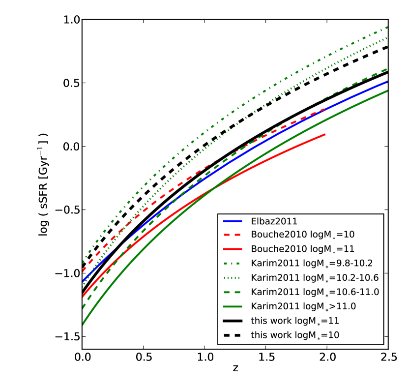
Figure 1.— Specific star formation rate (sSFR) versus redshift for different stellar masses. Three published forms are shown (Elbaz et al., 2011 in blue, Bouché et al., 2010 in red, and Karim et al., 2011 in green) as well as the relation adopted for this work in black.

2.1. Sample Selection

The EGNoG galaxies were selected from the parent samples (SDSS and COSMOS) to be as representative as possible of the ‘main sequence’ (MS) of star-forming galaxies. The main sequence is the tight correlation between $M_{*}$ and SFR that has been observed over a large range of redshifts: e.g. $z\approx 0$ (Brinchmann et al., 2004), $z\sim 0.2-1$ (Noeske et al., 2007), $z\sim 1-2$ (Elbaz et al., 2007; Daddi et al., 2007; Pannella et al., 2009), $z\sim 3-4$ (Daddi et al., 2009; Magdis et al., 2010) (see also the summary of recent results in Dutton et al., 2010). The sSFR increases with redshift, tracing the increase in the cosmological dark matter (and cold baryons, fuel for star formation) accretion rate onto halos (Bouché et al., 2010). Building on these observations, a few authors have attempted to describe the main sequence relation at all redshifts with one form. Figure 1 shows the functional forms of the specific star formation rate (sSFR$\equiv\mathrm{SFR}/M_{*}$) as a function of redshift reported by three papers: Bouché et al. (2010), Karim et al. (2011) and Elbaz et al. (2011). Bouché et al. (2010) suggest that existing literature data are well-fit by the form sSFR $\propto M_{*}^{-0.2}(1+z)^{2.7}$ for $z=0-2$. Karim et al. (2011) use a deep 3.6 $\mu$m selected sample of galaxies from the COSMOS field, with average SFRs determined from stacked 1.4 GHz radio continuum emission. Like Bouché et al. (2010), they find the sSFR to be a function of stellar mass, with galaxies with lower stellar masses having higher specific star formation rates. Specifically, the authors find sSFR $\propto M_{*}^{-0.4}(1+z)^{3.5}$ (on average) for star-forming galaxies at $z=0-3$ (in Figure 1, we plot the sSFR fit for each of the Karim et al. (2011) mass bins individually). On the other hand, Elbaz et al. (2011) argue that observations at all redshifts are consistent with a sSFR independent of stellar mass. The authors use far-infrared observations from Herschel Space Observatory in conjunction with existing data on the GOODS-North and GOODS-South fields to fit the sSFR versus redshift, finding sSFR (Gyr^-1) $\propto t_{\mathrm{cosmic}}^{-2.2}$ for $z=0-3$ (where $t_{\mathrm{cosmic}}$ is the time since the Big Bang in Gyr). The sSFR forms from Bouché et al. (2010) (red) and Karim et al. (2011) (green) are shown for different stellar masses in Figure 1. As Elbaz et al. (2011) argues that the sSFR is independent of sSFR, only one curve (blue) is plotted.

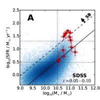
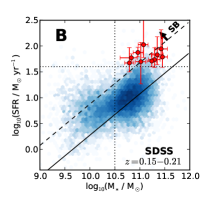
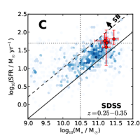
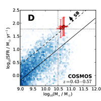
Figure 2.— Stellar mass versus SFR in each redshift bin. The redshift bin is indicated in the upper left corner of each panel. Red points with error bars show EGNoG galaxies. Dotted vertical and horizontal lines indicate the minimum $M_{*}$ and SFR, respectively, required for sample selection in each redshift bin (see text for full description). Blue shading shows the logarithm of the density (in the $M_{*}$-SFR plane) of star-forming galaxies from the parent dataset in the specified redshift range (given in the lower right corner). The redshift ranges plotted in bins B-D are slightly larger than the EGNoG redshift ranges, so that more data points may be included to better capture the behavior of the main sequence at each redshift. The solid black line indicates the main sequence (Equation 1) at the average redshift of the bin. The starburst criterion (Equation 2) is indicated by the black dashed line.

For this work, we are only concerned with the behavior of sSFR($z$) out to $z\approx 2.5$, but note that there is evidence for a flattening of this relation at $z\gtrsim 2-2.5$ (e.g. Stark et al., 2009; González et al., 2010; Reddy et al., 2012). For $z<2.5$, we adopt a sSFR relation which roughly agrees with the three forms described above. Specifically, we define

$$\mathrm{sSFR}_{\mathrm{MS}}(\mathrm{Gyr}^{-1})=0.07(1+z)^{3.2}\left(\frac{M_{*}}{10^{11}\ \mathrm{M}_{\odot}}\right)^{-0.2}$$ (1)

In Figure 1, this is plotted in black for $M_{*}=10^{10}$ M_⊙ (dashed) and $10^{11}$ M_⊙ (solid). We use this representative form of the sSFR to describe the main sequence of star-forming galaxies throughout this work.

To differentiate ‘starburst’ (SB) galaxies from normal main sequence galaxies, we adopt the quantitative definition given by Rodighiero et al. (2011), a study of PACS/Herschel observations of COSMOS and GOODS-South galaxies at $z=1.5-2.5$. Rodighiero et al. (2011) fit the main sequence population with a Gaussian distribution and define starbursts as outliers of this distribution. They find deviations from the Gaussian main sequence starting at a sSFR four times that of the main sequence. Therefore, we define starbursts as having

$$\mathrm{sSFR}_{\mathrm{SB}}>4\times\mathrm{sSFR}_{\mathrm{MS}}$$ (2)

In the selection of the EGNoG sample, we apply the following criteria in each redshift bin in order to identify non-interacting, star-forming galaxies lying as close to the main sequence as possible. At $z\lesssim 0.3$ (bins A-C), star-forming galaxies were selected (rejecting sources with AGN) using the cut from Kauffmann et al. (2003) in the BPT line-ratio diagram (Baldwin et al., 1981). We did not extend this criterion to bin D at $z\approx 0.5$ since the Kauffmann et al. (2003) dataset only covers $z=0.02-0.3$. Obviously interacting galaxies were excluded via visual inspection of the SDSS or COSMOS optical images. However, some interacting galaxies may remain in the sample due to the difficulty of identification at the modest resolution of the SDSS images.

Practical considerations imposed the following further constraints. From the SDSS dataset, we only used spectroscopically targeted galaxies, for which spectroscopic redshifts, stellar masses and SFRs were available from the MPA-JHU group. We required a spectroscopic redshift so that the error in the redshift is small enough to ensure that CO emission would be captured within the observed bandwidth. We excluded galaxies with SFRs below a minimum value estimated from the instrument sensitivity in each redshift range, assuming a molecular gas depletion time ($\tau_{\mathrm{mgas}}=M_{\mathrm{mgas}}/\mathrm{SFR}$) of 2 Gyr (Leroy et al., 2008), a Milky Way-like CO conversion factor (e.g. Dame et al., 2001) and (for bins C and D) a CO($J=3\rightarrow 2$) to CO($J=1\rightarrow 0$) line ratio ($r_{31}$) of 0.6 (Aravena et al., 2010). Note that this is close to $r_{31}=0.5$, found in the EGNoG bin C galaxies at $z\approx 0.3$ (see Bauermeister et al., 2013). In bin A, we used two SFR cutoffs since this bin is composed of two subsamples: high-SFR galaxies (EGNoG A1-A6) observed as a pilot study for the EGNoG survey, and a lower-SFR cutoff sample (EGNoG A7-A13) that is more representative of the main sequence. Finally, in order to restrict our selection to the main sequence at the SFRs probed, we required a minimum stellar mass of $10^{10.5}$ M_⊙.

In each redshift bin, the EGNoG galaxies were selected randomly from the subset of the parent sample that satisfied the constraints discussed above. Figure 2 shows stellar mass versus SFR in each of the four redshift bins. EGNoG galaxies are indicated by the red points with error bars. The vertical and horizontal dotted lines indicate the minimum $M_{*}$ and SFR, respectively, required for sample selection in each redshift bin. Galaxy C1 lies below the minimum SFR for bin C because it is a duplicate source in the SDSS catalog and was selected based on the higher SFR. The average SFR of the duplicate entries lies below the minimum SFR for bin C. The blue shading indicates the (logarithm of the) density of points in the $M_{*}$ - SFR plane for all star-forming galaxies (spectroscopic targets only for the SDSS data, bins A-C) in the redshift range indicated in the lower right of each panel. The redshift ranges plotted for bins B-D are slightly larger than the EGNoG redshift ranges so that more points may be included to better capture the behavior of the main sequence at each redshift. The blue shading corresponds to approximately 100,000 galaxies at $z=0.05-0.1$, 15,000 galaxies at $z=0.15-0.21$, 1300 galaxies at $z=0.25-0.35$, and 14,000 galaxies at $z=0.43-0.57$. The main sequence of star-forming galaxies at each redshift is indicated by the solid black line, with the starburst cutoff indicated by the dashed black line. From bin A to bin C, the low-mass, low-SFR end of the main sequence becomes sparsely sampled as the number of spectroscopically targeted, star-forming galaxies available in the SDSS decreases. This effect is most dramatic in the bin C panel, where the sample of spectroscopically-targeted star-forming galaxies in the SDSS is an order of magnitude smaller than in the bin B redshift range. Conversely, the small area covered by the COSMOS survey results in a sparsely sampled high-mass end of the main sequence in the bin D panel.

The result of our sample selection is that the EGNoG galaxies generally lie at the high-$M_{*}$, high-SFR end of the main sequence of star-forming galaxies. Our starburst criterion suggests that roughly half of the galaxies in each of bins A and B, and all of the bin D galaxies are starbursts. All four bin C galaxies lie below the starburst cut. In each redshift bin, the EGNoG galaxies lie roughly within the width of the scatter around the main sequence. The starburst classification of some of the EGNoG galaxies will be considered further in Section 5.

3. CARMA Observations

Each of the 31 EGNoG galaxies was observed in at least one rotational transition of the CO molecule: galaxies in bins A, B and C were observed in CO($J=1\rightarrow 0$) ($\nu_{\mathrm{rest}}=115.3$ GHz, $\nu_{\mathrm{obs}}\approx 107$, 98 and 88 GHz respectively); galaxies in bins C and D were observed in CO($J=3\rightarrow 2$) ($\nu_{\mathrm{rest}}=345.9$ GHz, $\nu_{\mathrm{obs}}\approx 266$ and 230 GHz respectively). At each frequency, each galaxy was observed over several different days. Each dataset includes observations of a nearby quasar for phase calibration (taken every 15-20 minutes), a bright quasar for passband calibration and either a planet (Uranus, Neptune or Mars) or MWC349 for flux calibration (in most cases).

The reduction of all observations for this survey was carried out within the EGN data reduction infrastructure (based on the MIS pipeline; Pound & Teuben, 2012) using the Multichannel Image Reconstruction, Image Analysis and Display (MIRIAD, Sault et al., 2011) package for radio interferometer data reduction. Our data analysis also used the miriad-python software package (Williams et al., 2012). The data were flagged, passband-calibrated and phase calibrated in the standard way. Final images were created using invert with options=mosaic to properly handle and correct for the three different primary beam patterns. All observations are single-pointing. We describe the CO($J=1\rightarrow 0$) and CO($J=3\rightarrow 2$) observations individually below. A full description of the data reduction and flux measurement is given in Appendix B.

3.1. CO($J=1\rightarrow 0$)

The CO($J=1\rightarrow 0$) transition lies in the 3 mm band of CARMA (single-polarization, linearly polarized feeds) for galaxies in bins A, B and C. The line was observed with at least three overlapping 500 MHz bands, covering $\approx$ 4200, 4600 and 5000 km s^-1 total, at 35, 39 and 42 km s^-1 resolution for galaxies in bins A, B and C, respectively.

Bin A galaxies were observed during three time periods: October to November 2010, April to May 2011 and February 2012. All data were taken in CARMA’s C configuration, with $26-370$ m baselines yielding a typical synthesized beam of $2.0\arcsec\times 1.5\arcsec$ at 107 GHz. These observations are sensitive to spatial scales up to $\approx 22\arcsec$, which is sufficient for most galaxies in the sample but may resolve out some large scale structure in the largest galaxies. However, since molecular gas is centrally concentrated, we expect any under-estimation of the flux to be minimal. (In D and E configuration in the 3mm band, we are sensitive to sufficiently large spatial scales so that we expect to recover all of the flux.) Each galaxy was observed for 2-3 hours (time on-source), yielding final data cubes with a typical rms noise of $5-10$ mJy beam^-1 in 35 km s^-1 channels.

Bin B sources were observed from August to November 2011 and April 2012 in CARMA’s D configuration, with $11-150$ m baselines yielding a typical synthesized beam of $4.9\arcsec\times 3.9\arcsec$ at 98 GHz. Supplementary observations were made of B1, B2, B3 and B7 in CARMA’s C array in February 2012, which resulted in a synthesized beam of $3.0\arcsec\times 2.3\arcsec$ in the final maps combining data from both array configurations. Each galaxy was observed in D configuration for approximately 7 hours (time on-source), resulting in a typical rms noise of 2.5 mJy beam^-1 in 39 km s^-1 channels in the final cube.

Bin C observations were made from August to November 2011 in CARMA’s D configuration, with a typical synthesized beam of $4.8\arcsec\times 3.9\arcsec$ at 88 GHz. Each galaxy was observed for 20 to 30 hours (time on-source), yielding final cubes with a typical rms noise of $1.2$ mJy beam^-1 in 42 km s^-1 channels.

The flux scale in each dataset is set by the flux of the phase calibrator, which is determined from the flux calibrator. For the fluxes used, see Appendix B.

Of the 27 galaxies observed in the CO($J=1\rightarrow 0$) line, we detected 24 easily, with 3 non-detections in bin A. The $uv$-spectra of the detected galaxies are shown in Appendix D.

3.2. CO($J=3\rightarrow 2$)

The CO($J=3\rightarrow 2$) transition lies in the CARMA 1 mm band (dual-polarization, circularly polarized feeds) for galaxies in bins C and D. We again observed the line with at least three overlapping 500 MHz bands, covering $\approx$ 1500 and 1700 km s^-1 total, at 14 and 15 km s^-1 resolution, for galaxies in bins C and D respectively.

Bin C observations were carried out in CARMA’s E configuration during August 2011 and D configuration during April 2012. Source C4 was observed entirely in E configuration, while the other three sources were observed mostly in D configuration. The E configuration has $8-66$ m baselines yielding a typical synthesized beam of $3.2\arcsec\times 2.5\arcsec$ at 266 GHz. The D configuration has $11-150$ m baselines yielding a typical synthesized beam of $1.7\arcsec\times 1.5\arcsec$ at 266 GHz. Each galaxy was observed for 2 to 6.5 hours (time on-source), yielding final cubes with a rms noise of 5-10 mJy beam^-1 in 42 km s^-1 channels.

Bin D observations were carried out in CARMA’s E and D configuration during August 2011 and April to June 2012, respectively. In E configuration, a typical synthesized beam is $4.2\arcsec\times 3.6\arcsec$ at 230 GHz. In D configuration, a typical synthesized beam is $2.5\arcsec\times 1.7\arcsec$ at 230 GHz. Galaxies D1 and D2 were observed in both D and E configuration for approximately 10 hours (time on-source) total, yielding final cubes with a rms noise of $\approx 7$ mJy beam^-1 in 48 km s^-1 channels. Galaxies D3 and D4 were observed in D configuration for approximately 3 hours (time on-source), yielding final cubes with a rms noise of $\approx 10$ mJy beam^-1 in 48 km s^-1 channels.

In bin C, sources C2, C3 and C4 were detected at the $\approx 5\sigma$ level in the CO($J=3\rightarrow 2$) line. However, C1, with its wide velocity profile (observed in the CO($J=1\rightarrow 0$) line), was only marginally detected and we provide an upper limit on the CO($J=3\rightarrow 2$) flux. The $uv$-spectra for the bin C galaxies are shown in Appendix D. In bin D, we do not significantly detect any of the four galaxies, and list only upper limits. The bin D galaxies are discussed further in Section 4.3

4. Results

4.1. CO Emission Maps and Molecular Gas Masses

Table 3 presents the quantities we derive from the CO observations. The CO line luminosity is calculated from the line flux ($S_{\mathrm{CO}}$ in Jy km s^-1, calculated as described in Section B.2) following

$$L_{\mathrm{CO}}^{\prime}=3.25\times 10^{7}\ S_{\mathrm{CO}}\ \nu_{\mathrm{obs}}^{-2}\ r_{\mathrm{com}}^{2}(1+z)^{-1}$$ (3)

(see the review by Solomon & Vanden Bout, 2005), where $\nu_{\mathrm{obs}}$ is in GHz and $r_{\mathrm{com}}$ is the comoving distance in Mpc. The units of $L_{\mathrm{CO}}^{\prime}$ are K km s^-1 pc². We report the measurement error for $S_{\mathrm{CO}}$. The error reported for $L_{\mathrm{CO}}^{\prime}$ includes both the measurement error of $S_{\mathrm{CO}}$ and a 30% systematic error, added in quadrature (see Section B.2 for more details).

The center velocity, $v_{\mathrm{center}}$, is the flux-weighted average velocity of the galaxy-integrated spectrum ($v=0$ at the redshift in Table 2). The error reported is the standard deviation of the $v_{\mathrm{center}}$ values found with the three flux measurement methods and different channel averaging described in Section B.2. The reported velocity width ($\Delta V$) is the full width of the emission, where ‘source’ velocity channels are selected by eye. We give the velocity width of a single channel as the error.

In the case of a non-detection (galaxies A4, A6, A12, D1, D2, D3, and D4; indicated by ^a in Table 3), we estimate a $3\sigma$ upper limit on $S_{\mathrm{CO}}$ from the noise in the channel maps and a maximum velocity width motivated by detections at that redshift: 600 km s^-1 in bin A and 400 km s^-1 in bin D. For the CO($J=3\rightarrow 2$) line in galaxy C1, while the CO($J=3\rightarrow 2$) channel maps did not show evidence of a source upon visual inspection, an integrated spectrum made of a circular region $4.5\arcsec$ in radius at the center of the image suggests a $3\sigma$ detection. We calculate an upper limit on the line flux (and related quantities) from this spectrum, over the velocities of the CO($J=1\rightarrow 0$) line in C1.

Name

Jup

$S_{\mathrm{CO}}$

$v_{\mathrm{center}}$

$\Delta V$

$L_{\mathrm{CO}}^{\prime}$

sSFR

$M_{\mathrm{mgas}}$

$f_{\mathrm{mgas}}$

$\tau_{\mathrm{dep}}$

(Jy km s-1)

(km s-1)

(km s-1)

($10^{9}$ K km s-1 pc2)

class

($10^{9}M_{\odot}$)

(Gyr)

A1

1

10.75 $\ \pm\$

2.99

33.7 $\ \pm\$

27.3

428.0 $\ \pm\$

71.3

4.76 $\ \pm\$

1.95

SB

5.18 $\ \pm\$

2.12

$0.09^{+0.04}_{-0.04}$

$0.17^{+0.09}_{-0.08}$

A2

1

14.40 $\ \pm\$

2.55

30.5 $\ \pm\$

12.6

281.2 $\ \pm\$

35.2

4.44 $\ \pm\$

1.55

norm

19.32 $\ \pm\$

6.73

$0.17^{+0.06}_{-0.06}$

$0.68^{+0.27}_{-0.27}$

A3

1

17.94 $\ \pm\$

2.07

22.8 $\ \pm\$

6.8

552.5 $\ \pm\$

34.5

3.22 $\ \pm\$

1.03

norm

14.01 $\ \pm\$

4.50

$0.12^{+0.04}_{-0.04}$

$0.65^{+0.29}_{-0.29}$

A4a

1

5.98 $\ \pm\$

1.98

0.0 $\ \pm\$

0.0

600.0 $\ \pm\$

0.0

2.25 $\ \pm\$

1.01

SB

2.45 $\ \pm\$

1.09

$0.03^{+0.01}_{-0.01}$

$0.05^{+0.02}_{-0.02}$

A5

1

23.22 $\ \pm\$

3.90

-60.3 $\ \pm\$

9.8

492.0 $\ \pm\$

35.1

7.12 $\ \pm\$

2.45

SB

7.75 $\ \pm\$

2.66

$0.07^{+0.03}_{-0.03}$

$0.18^{+0.07}_{-0.07}$

A6a

1

3.65 $\ \pm\$

1.23

0.0 $\ \pm\$

0.0

600.0 $\ \pm\$

0.0

1.24 $\ \pm\$

0.56

SB

1.35 $\ \pm\$

0.61

$0.02^{+0.01}_{-0.01}$

$0.04^{+0.02}_{-0.02}$

A7

1

6.72 $\ \pm\$

1.52

49.2 $\ \pm\$

31.9

319.0 $\ \pm\$

106.3

2.58 $\ \pm\$

0.97

SB

2.81 $\ \pm\$

1.05

$0.04^{+0.02}_{-0.02}$

$0.07^{+0.03}_{-0.03}$

A8

1

4.52 $\ \pm\$

1.35

-61.0 $\ \pm\$

20.5

357.3 $\ \pm\$

71.5

2.10 $\ \pm\$

0.89

norm

9.14 $\ \pm\$

3.87

$0.05^{+0.03}_{-0.02}$

$1.22^{+0.70}_{-0.70}$

A9

1

5.68 $\ \pm\$

1.42

-7.1 $\ \pm\$

17.7

420.3 $\ \pm\$

70.1

1.59 $\ \pm\$

0.62

norm

6.92 $\ \pm\$

2.70

$0.16^{+0.06}_{-0.06}$

$1.86^{+0.91}_{-0.91}$

A10

1

7.88 $\ \pm\$

3.16

4.3 $\ \pm\$

17.0

274.4 $\ \pm\$

68.6

1.11 $\ \pm\$

0.56

norm

4.83 $\ \pm\$

2.42

$0.08^{+0.04}_{-0.04}$

$0.94^{+0.54}_{-0.54}$

A11

1

6.89 $\ \pm\$

0.98

-10.5 $\ \pm\$

11.2

419.8 $\ \pm\$

70.0

1.86 $\ \pm\$

0.62

norm

8.09 $\ \pm\$

2.69

$0.13^{+0.05}_{-0.04}$

$0.91^{+0.39}_{-0.39}$

A12a

1

3.50 $\ \pm\$

1.16

0.0 $\ \pm\$

0.0

600.0 $\ \pm\$

0.0

1.59 $\ \pm\$

0.71

norm

6.92 $\ \pm\$

3.09

$0.16^{+0.07}_{-0.07}$

$2.03^{+1.45}_{-1.45}$

A13

1

21.89 $\ \pm\$

4.12

-27.3 $\ \pm\$

8.9

563.5 $\ \pm\$

35.2

7.15 $\ \pm\$

2.53

norm

31.12 $\ \pm\$

11.02

$0.21^{+0.08}_{-0.07}$

$2.67^{+1.63}_{-1.63}$

B1

1

11.35 $\ \pm\$

0.62

-23.1 $\ \pm\$

4.0

615.4 $\ \pm\$

38.5

18.60 $\ \pm\$

5.67

norm

80.95 $\ \pm\$

24.68

$0.23^{+0.08}_{-0.07}$

$0.92^{+0.60}_{-0.60}$

B2

1

7.32 $\ \pm\$

0.40

25.5 $\ \pm\$

11.7

581.1 $\ \pm\$

38.7

13.20 $\ \pm\$

4.03

norm

57.45 $\ \pm\$

17.52

$0.23^{+0.08}_{-0.07}$

$1.05^{+0.54}_{-0.54}$

B3

1

4.49 $\ \pm\$

0.35

-23.1 $\ \pm\$

6.6

378.9 $\ \pm\$

37.9

5.97 $\ \pm\$

1.85

SB

6.50 $\ \pm\$

2.01

$0.10^{+0.03}_{-0.03}$

$0.14^{+0.08}_{-0.08}$

B4

1

4.81 $\ \pm\$

0.20

-25.6 $\ \pm\$

5.2

457.6 $\ \pm\$

38.1

6.99 $\ \pm\$

2.12

SB

7.61 $\ \pm\$

2.30

$0.07^{+0.03}_{-0.02}$

$0.15^{+0.26}_{-0.10}$

B5

1

6.61 $\ \pm\$

0.22

16.1 $\ \pm\$

2.5

307.6 $\ \pm\$

38.5

10.70 $\ \pm\$

3.23

norm

46.57 $\ \pm\$

14.06

$0.21^{+0.07}_{-0.06}$

$0.91^{+0.38}_{-0.38}$

B6

1

3.52 $\ \pm\$

0.31

-133.6 $\ \pm\$

16.4

343.7 $\ \pm\$

38.2

5.22 $\ \pm\$

1.63

SB

5.68 $\ \pm\$

1.78

$0.08^{+0.05}_{-0.03}$

$0.10^{+0.03}_{-0.03}$

B7

1

5.97 $\ \pm\$

0.30

-40.9 $\ \pm\$

4.9

497.0 $\ \pm\$

38.2

9.01 $\ \pm\$

2.74

norm

39.21 $\ \pm\$

11.93

$0.12^{+0.04}_{-0.04}$

$0.64^{+0.42}_{-0.42}$

B8

1

2.25 $\ \pm\$

0.33

-34.8 $\ \pm\$

20.4

382.5 $\ \pm\$

76.5

3.41 $\ \pm\$

1.14

SB

3.71 $\ \pm\$

1.24

$0.03^{+0.01}_{-0.01}$

$0.03^{+0.03}_{-0.03}$

B9

1

3.91 $\ \pm\$

0.27

-18.6 $\ \pm\$

5.9

459.5 $\ \pm\$

38.3

6.03 $\ \pm\$

1.86

norm

26.24 $\ \pm\$

8.08

$0.11^{+0.04}_{-0.04}$

$0.39^{+0.25}_{-0.25}$

B10

1

5.25 $\ \pm\$

0.22

27.1 $\ \pm\$

2.6

270.9 $\ \pm\$

38.7

9.28 $\ \pm\$

2.81

SB

10.10 $\ \pm\$

3.06

$0.10^{+0.03}_{-0.03}$

$0.13^{+0.05}_{-0.05}$

C1

1

2.05 $\ \pm\$

0.34

-84.9 $\ \pm\$

18.1

542.2 $\ \pm\$

41.7

8.25 $\ \pm\$

2.83

norm

35.90 $\ \pm\$

12.31

$0.17^{+0.06}_{-0.06}$

$0.93^{+2.09}_{-0.69}$

C2

1

2.35 $\ \pm\$

0.10

-6.7 $\ \pm\$

1.2

253.7 $\ \pm\$

42.3

10.70 $\ \pm\$

3.24

norm

46.57 $\ \pm\$

14.11

$0.23^{+0.18}_{-0.07}$

$0.81^{+0.39}_{-0.39}$

C3

1

4.39 $\ \pm\$

0.09

-24.7 $\ \pm\$

5.7

384.0 $\ \pm\$

42.3

21.70 $\ \pm\$

6.53

norm

94.44 $\ \pm\$

28.40

$0.25^{+0.15}_{-0.07}$

$1.45^{+0.77}_{-0.77}$

C4

1

3.01 $\ \pm\$

0.11

17.3 $\ \pm\$

13.0

292.5 $\ \pm\$

41.8

12.30 $\ \pm\$

3.72

norm

53.53 $\ \pm\$

16.18

$0.23^{+0.10}_{-0.07}$

$1.06^{+0.45}_{-0.45}$

C1a

3

9.02 $\ \pm\$

2.65

-49.9 $\ \pm\$

7.3

542.3 $\ \pm\$

23.4

4.03 $\ \pm\$

1.69

norm

35.08 $\ \pm\$

14.73

$0.17^{+0.07}_{-0.07}$

$0.91^{+2.05}_{-0.71}$

C2

3

8.39 $\ \pm\$

1.12

19.5 $\ \pm\$

8.2

169.2 $\ \pm\$

42.3

4.25 $\ \pm\$

1.40

norm

36.99 $\ \pm\$

12.15

$0.19^{+0.16}_{-0.07}$

$0.64^{+0.32}_{-0.32}$

C3

3

13.46 $\ \pm\$

1.56

-14.0 $\ \pm\$

7.8

426.7 $\ \pm\$

42.7

7.39 $\ \pm\$

2.38

norm

64.32 $\ \pm\$

20.69

$0.18^{+0.12}_{-0.06}$

$0.99^{+0.53}_{-0.53}$

C4

3

11.88 $\ \pm\$

1.22

33.5 $\ \pm\$

5.0

250.7 $\ \pm\$

41.8

5.41 $\ \pm\$

1.72

norm

47.09 $\ \pm\$

14.93

$0.21^{+0.10}_{-0.07}$

$0.93^{+0.41}_{-0.41}$

D1a

3

3.36 $\ \pm\$

1.12

0.0 $\ \pm\$

0.0

400.0 $\ \pm\$

0.0

4.38 $\ \pm\$

1.96

SB

9.53 $\ \pm\$

4.27

$0.19^{+0.09}_{-0.08}$

$0.15^{+0.20}_{-0.11}$

D2a

3

2.73 $\ \pm\$

0.91

0.0 $\ \pm\$

0.0

400.0 $\ \pm\$

0.0

4.45 $\ \pm\$

2.00

SB

9.68 $\ \pm\$

4.34

$0.17^{+0.08}_{-0.07}$

$0.13^{+0.18}_{-0.10}$

D3a

3

3.39 $\ \pm\$

1.13

0.0 $\ \pm\$

0.0

400.0 $\ \pm\$

0.0

4.36 $\ \pm\$

1.96

SB

9.49 $\ \pm\$

4.25

$0.15^{+0.08}_{-0.07}$

$0.12^{+0.16}_{-0.09}$

D4a

3

5.19 $\ \pm\$

1.73

0.0 $\ \pm\$

0.0

400.0 $\ \pm\$

0.0

6.88 $\ \pm\$

3.09

SB

14.97 $\ \pm\$

6.71

$0.21^{+0.10}_{-0.09}$

$0.20^{+0.27}_{-0.14}$

Table 3Properties of the CO emission of the EGNoG galaxies (described in Section 4.1). See Section B.2 for a description of the errors.
^a CO quantities are upper limits.

The molecular gas mass ($M_{\mathrm{mgas}}$) is calculated from $L_{\mathrm{CO}}^{\prime}$ according to

$$M_{\mathrm{mgas}}=1.36~{}\alpha_{\mathrm{CO}}~{}L_{\mathrm{CO(J-(J-1))}}^{\prime}~{}/~{}r_{\mathrm{J1}}$$ (4)

where $\alpha_{\mathrm{CO}}$ is the CO($J=1\rightarrow 0$) luminosity to H₂ mass conversion factor (akin to $X_{\mathrm{CO}}$) and the factor of 1.36 accounts for Helium to yield the total molecular gas mass. $r_{\mathrm{J1}}$ is the ratio of the CO line luminosities: $r_{J1}=L_{\mathrm{CO}}^{\prime}(J\rightarrow J-1)/L_{\mathrm{CO}}^{\prime}(1\rightarrow 0)$. In the calculation of the molecular gas mass from the CO($J=3\rightarrow 2$) luminosity (bin C and D observations), we use $r_{31}=0.5$, observed in the EGNoG bin C galaxies (Bauermeister et al., 2013). We use an $\alpha_{\mathrm{CO}}$ value selected according to the starburst classification described by Equations 1 and 2. For galaxies classified as starburst, we use the value observed in local ULIRGs: $\alpha_{\mathrm{CO}}(\mathrm{ULIRG})=0.8$ M_⊙ (K km s^-1 pc²)^-1 (Scoville et al., 1997; Downes & Solomon, 1998). For all other galaxies, we use a Milky Way-like conversion factor, $\alpha_{\mathrm{CO}}(\mathrm{MilkyWay})=3.2$ M_⊙ (K km s^-1 pc²)^-1 (e.g. Dame et al., 2001). This classification (SB or norm), and the molecular gas mass calculated using the corresponding $\alpha_{\mathrm{CO}}$ is reported for each galaxy in Table 3. There is of course considerable uncertainty in the appropriate $\alpha_{\mathrm{CO}}$ value, but we do not reflect this uncertainty in the error in the molecular gas mass. The error in $M_{\mathrm{mgas}}$ is calculated by propagating the error in $L_{\mathrm{CO}}^{\prime}$. The classification of galaxies using the specific star formation rate is described in more detail in Section 5.2. In Section 5.5, we discuss the use of a bimodal prescription for $\alpha_{\mathrm{CO}}$ in this work and the the possibility of a continuously varying conversion factor.

We report the molecular gas fraction and the molecular gas depletion time in the last two columns of Table 3. In keeping with previous work, we define the molecular gas fraction ($f_{\mathrm{mgas}}$) as the fraction of baryonic matter (ignoring atomic and ionized gas):

$$f_{\mathrm{mgas}}=\frac{M_{\mathrm{mgas}}}{M_{*}+M_{\mathrm{mgas}}}$$ (5)

The molecular gas depletion time ($\tau_{mgas}$) represents the time it would take to consume all the available molecular gas at the current star formation rate, defined:

$$\tau_{\mathrm{dep}}=\frac{M_{\mathrm{mgas}}}{SFR}$$ (6)

The errors in both of these quantities include both the error in the CO luminosity and the error in the stellar mass or SFR.

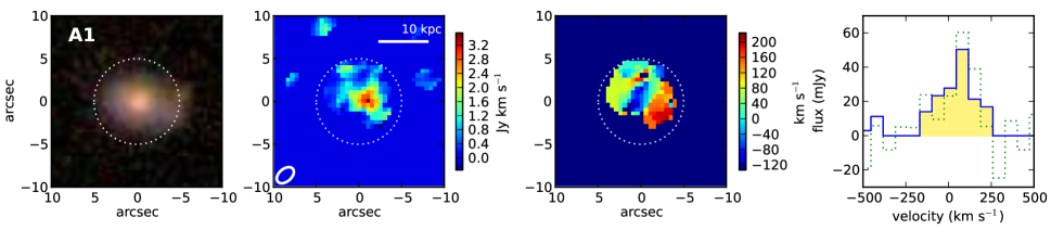
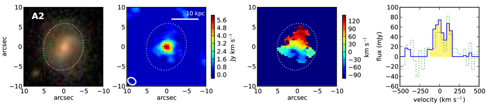
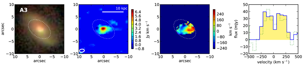
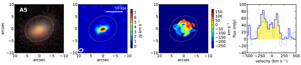
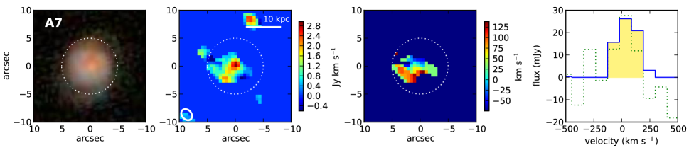
Figure 3.— Integrated CO emission maps for detected bin A galaxies, part 1. The left panel shows the optical image with the galaxy name in the upper left. The moment 0 and moment 1 maps are displayed in the left middle and right middle panels respectively. The dotted white ellipse indicates the source region. In the moment 0 map, the synthesized beam is indicated by the solid white ellipse in the lower left corner and a 10 kpc scale bar is given in the top right. The moment 1 map is masked outside of the source region ellipse for clarity. The far right panel shows the integrated spectrum of the galaxy: the solid blue line is calculated with masking, the dotted green line is without.

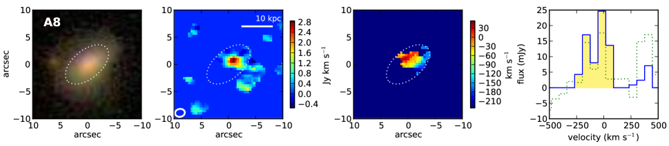
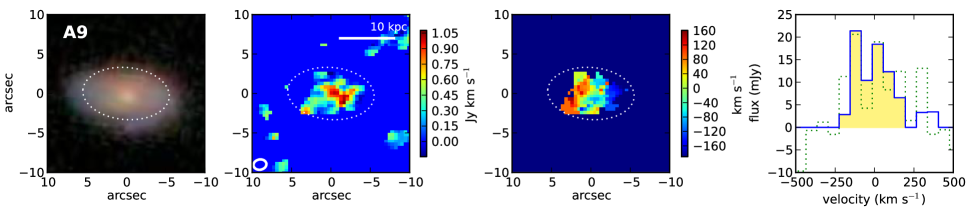
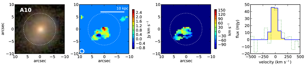
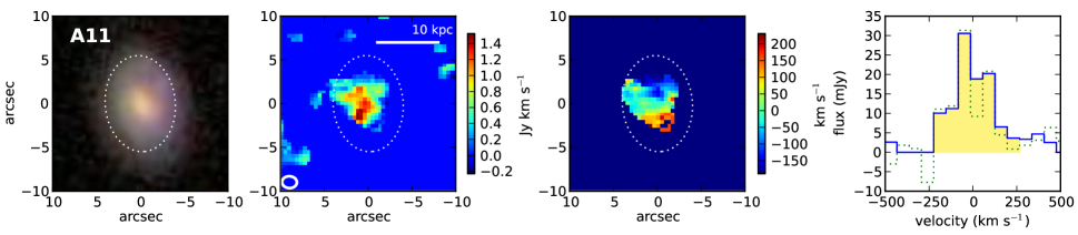
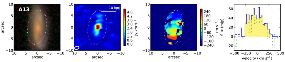
Figure 4.— Integrated CO emission maps for detected bin A galaxies, part 2. Same as Figure 3.

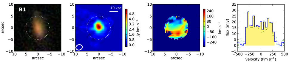
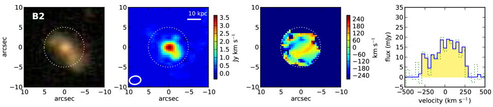
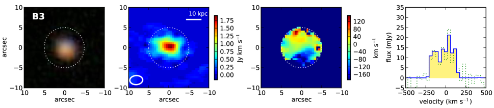
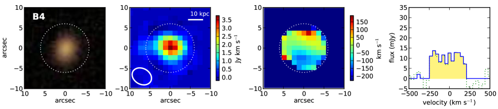
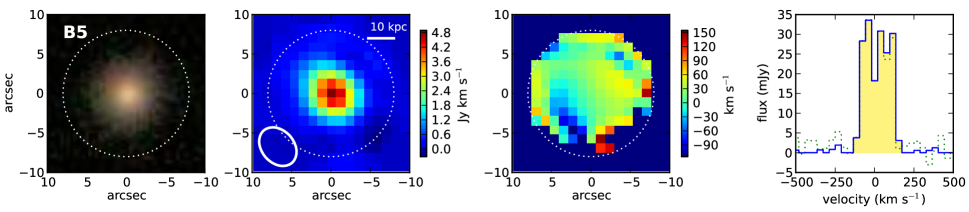
Figure 5.— Integrated CO emission maps for bin B galaxies, part 1. Same as Figure 3.

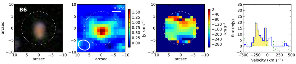
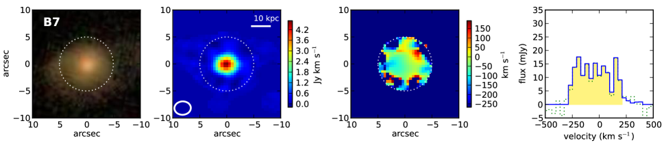
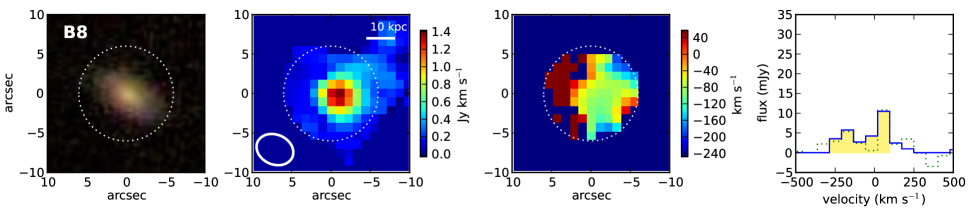
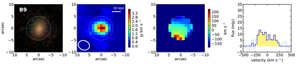
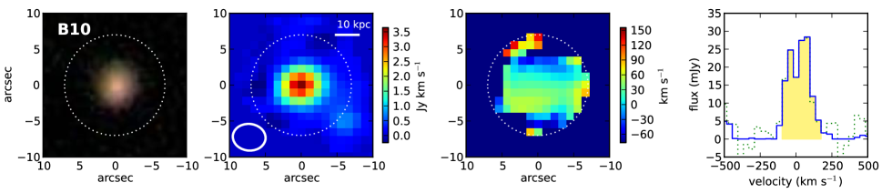
Figure 6.— Integrated CO emission maps for bin B galaxies, part 2. Same as Figure 3.

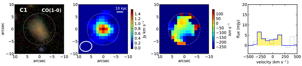
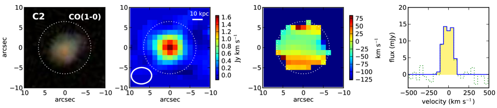
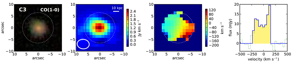
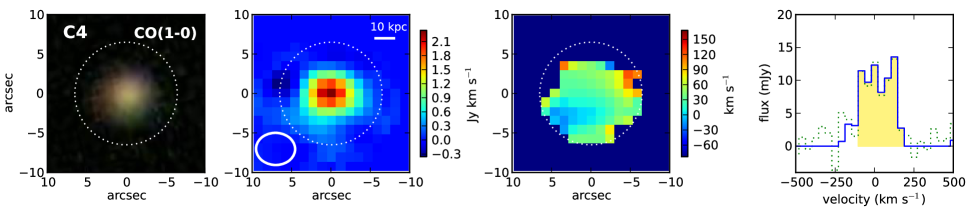
Figure 7.— Integrated CO emission maps for bin C galaxies in the CO($J=1\rightarrow 0$) line. Same as Figure 3.

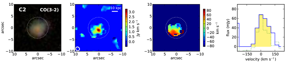
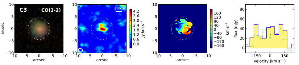
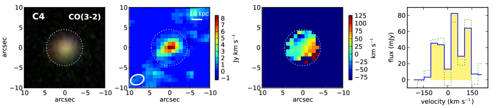
Figure 8.— Integrated CO emission maps for (detected) bin C galaxies in the CO($J=3\rightarrow 2$) line. Same as Figure 3.

The integrated CO emission maps of all detected galaxies are presented in Figures 3 - 8. For each galaxy, the optical image (from SDSS) is in the left-most panel, the moment 0 (total intensity) map is in the left middle panel, the moment 1 (intensity-weighted mean velocity) map is in the right middle panel, and the integrated spectrum is in the far right panel. The dotted white ellipse shows the region in which pixels were summed (if not masked; see Section B.2 for details). For clarity, we have additionally masked the moment 1 map outside of the source region (dotted white ellipse) in Figures 3 - 8. The white bar in the moment 0 map shows the angular size of 10 kpc at the redshift of the galaxy. In the far right panel, the solid blue line shows the masked spectrum and the dotted green line shows the unmasked spectrum. Channels containing source emission are shaded yellow.

The moment maps are produced using the $2\sigma$ clipped smooth mask method (see Section B.2). The moment 0 map is a simple sum of the masked cube in the ‘source’ velocity channels. The moment 1 map is produced by summing the masked cube multiplied by the velocity in each channel, then normalizing by the moment 0 value. Thus, the color in the moment 1 map indicates the intensity-weighted mean velocity in each pixel. The moment 1 map is only calculated in pixels which have a positive moment 0 value. Moment 1 pixels with values outside the velocity range covered by the source channels are masked.

In most of the bin A galaxies, we spatially resolve the CO disk, illustrated by a velocity gradient across the emission region in the moment 1 map (indicative of a rotating disk). The morphology of the bin A CO emission is discussed further in Section 4.2. The bin B galaxies which were observed only in D configuration are spatially unresolved. However, galaxies B1, B2, B3 and B7 were observed in C configuration as well, increasing the resolution by roughly a factor of 2. Of these four, galaxies B1 and B3 show evidence for ordered rotation but are only marginally resolved. Bin C galaxies are spatially unresolved in the CO($J=1\rightarrow 0$) line and marginally resolved in the CO($J=3\rightarrow 2$) line. The CO($J=3\rightarrow 2$) moment 1 maps of the galaxies C2, C3 and C4 are suggestive of a rotating disk of gas. Bin D galaxies are not detected, but would be unresolved based on the sizes of the stellar disks.

4.2. Morphology of the Low-Redshift Sample

For the EGNoG galaxies in redshift bin A, the spatial resolution of the CO observations allows us to comment on the morphology of the molecular gas disk at $z=0.05-0.1$. The integrated CO intensity maps in Figures 3 and 4 are suggestive of irregular morphology at first glance. However, due to the modest signal to noise ratio of these observations, it is difficult to infer the true shape of the underlying CO emission.

To determine the effect of a modest signal to noise ratio on our CO emission maps, we produced a simple model disk galaxy at $z=0.08$, inserted it into noise-only $uv$ data channels from a bin A galaxy dataset and processed the data as we did the real data. We used a Milky-Way-like rotation curve, linear in the central 1 kpc, flat outside. The distribution of the CO emission is exponential, with a scale radius of 3 kpc. We varied the total flux, rotation velocity of the flat part of the rotation curve ($v_{\mathrm{flat}}$), inclination angle ($i$) and physical radius of the molecular gas disk ($R_{\mathrm{CO}}$). Models M1 to M4, shown in Figure 9, are representative of the results of varying all four parameters within reasonable ranges. The parameters used in the four models are listed in Table 4.

The ‘observed’ model maps (right two panels in Figure 9) suggest that at the signal to noise level typical of our bin A data, irregularities in the CO emission maps do not necessarily indicate an underlying irregular structure in the molecular gas disk. In most cases, our observations are consistent with the CO in the bin A galaxies being ordered in a rotating disk. We conclude that deeper observations would be required to investigate the detailed morphology of the molecular gas disks in these systems.

Two exceptions are galaxies A3 and A8, which exhibit disturbed morphologies that are not likely the result of low signal to noise ratios. Both galaxies show rotating molecular gas disks misaligned with the major axis of the optical disk, as well as CO emission outside the optical disk. These two galaxies are discussed in detail in Appendix E.

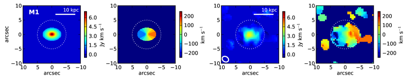
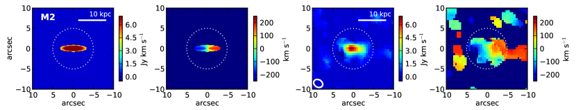
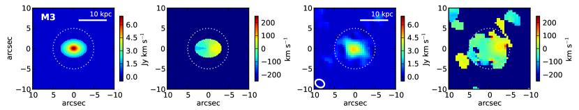
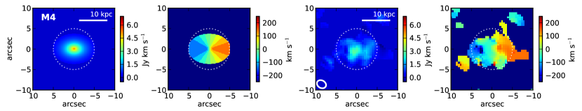
Figure 9.— Model galaxy maps. For each model (M1 - M4, parameters given in Table 4), the far left and left middle panels show the model galaxy moment 0 and moment 1 maps respectively. In the right middle and far right panels are the moment 0 and moment 1 maps from normal processing of the model galaxy inserted into noise-only data.

4.3. Non-Detections of the Bin D Galaxies

We do not detect CO($J=3\rightarrow 2$) in any of the four bin D galaxies at $z\approx 0.5$. The $3\sigma$ upper limits on $S_{\mathrm{CO}}$ are between 2.7 and 5.2 Jy km s^-1, assuming a total velocity width of 400 km s^-1. The spectra of the four bin D galaxies are shown in the top four panels of Figure 10 at a velocity resolution of $\approx 32$ km s^-1. The bottom panel shows the stacked spectrum, where each individual spectrum is weighted by the inverse of the variance. Note that the spectra are stacked centered at the spectroscopic redshifts given in Table 3, which have a typical uncertainty of 110 km s^-1. The stacked spectrum does not indicate a detection; we calculate a 3$\sigma$ upper limit of 1.5 Jy km s^-1 for a 400 km s^-1 wide signal.

	$i$	$v_{\mathrm{flat}}$	$R_{\mathrm{CO}}$	$S_{\mathrm{CO}}$
Model	(deg)	(km s-1)	(kpc)	(Jy km s-1)
M1	45	200	5	14
M2	75	200	5	14
M3	45	100	5	14
M4	45	200	8	14

Table 4Model parameters: inclination angle ($i$), rotation velocity of the flat part of the velocity curve ($v_{\mathrm{flat}}$), radius of the CO disk ($R_{\mathrm{CO}}$) and total CO flux ($S_{\mathrm{CO}}$).

To place these limits in context, we calculate the expected CO flux of a galaxy with SFR $\approx 70$ M_⊙ yr^-1, typical for the bin D galaxies. First we consider these galaxies to be normal, using a Milky way-like $\alpha_{\mathrm{CO}}$ and $r_{31}=0.5$. For $\tau_{\mathrm{mgas}}=0.77\pm 0.57$ Gyr (average from our literature sample; see Section 5.3), we expect a CO flux $S_{\mathrm{CO}}=1.2-8.4$ Jy km s^-1. Performing the same calculation using a starburst $\alpha_{\mathrm{CO}}$ and the starburst average $\tau_{\mathrm{mgas}}=0.07\pm 0.04$ Gyr (Section 5.3), we expect $S_{\mathrm{CO}}=0.76-2.7$ Jy km s^-1. We have used $r_{31}=0.5$ in this calculation but note that a larger value may be appropriate in a starburst system. We can further constrain the expected CO flux using the typical stellar mass ($\log(M_{*})=10.7$) and the expected molecular gas fraction (see Section 5.4). For $f_{\mathrm{mgas}}=0.03-0.4$, we expect $S_{\mathrm{CO}}=0.13-2.6$ Jy km s^-1 for normal galaxies or $S_{\mathrm{CO}}=0.5-11.0$ Jy km s^-1 for starburst galaxies. Note also that these estimates have an uncertainty of a factor of 1.5-2.5 from the uncertainty in the SFR and $M_{*}$ of the bin D galaxies, in addition to further uncertainty in the $r_{31}$ value.

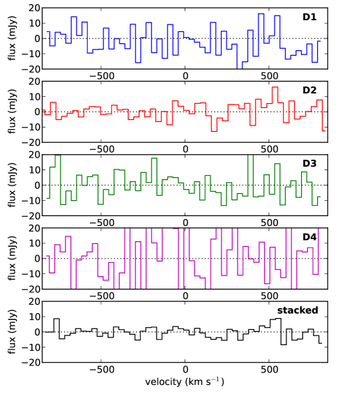
Figure 10.— Spectra of the four bin D sources within a circular region $2\arcsec$ in radius (top four panels), plus the stacked (average) spectrum, weighted by the inverse of the variance, in the bottom panel.

Considering the range of expected CO fluxes, four non-detections at the depth of these observations is not unreasonable. Given the large, overlapping ranges of expected CO fluxes for starburst and normal galaxies detailed above, we do not draw any conclusions about the gas consumption properties of the bin D galaxies based on these upper limits.

5. Discussion

We now look at the EGNoG galaxies in the context of starburst and normal galaxies at low and high redshift from the literature. We present the literature sample in the following section (Section 5.1), describe our identification and treatment of starburst and normal galaxies in the literature dataset (Section 5.2), then investigate the molecular gas depletion times in normal and starburst galaxies (Section 5.3) and the evolution of the molecular gas fraction with redshift (Section 5.4).

5.1. Literature Data

The local galaxies of our literature data compilation include normal spiral galaxies, LIRGs and ULIRGs. We include 22 galaxies from Leroy et al. (2008), 10 of which are defined by the authors to be dwarf galaxies ($M_{*}<10^{10}$ M_⊙). Leroy et al. (2008) present CO data from the HERACLES and BIMA SONG surveys, stellar masses estimated from the SINGS survey K-band luminosities, and star formation rates calculated from a combination of GALEX FUV and Spitzer 24 $\mu$m. We augment this dataset with 47 galaxies (26 of which have $M_{*}<10^{10}$ M_⊙) from the overlap of the H$\alpha$ survey by Kennicutt et al. (2008) and the CO sample (taken from the literature) of Obreschkow & Rawlings (2009). We estimate stellar masses, star formation rates and CO luminosities for these galaxies following Bothwell et al. (2009). For each galaxy, the stellar mass is calculated from the B-band luminosity using a mass-to-light ratio estimated using the B-V color (Bell & de Jong, 2001). The SFR is calculated from the H$\alpha$ flux via the relation given by Kennicutt (1998a), using an extinction correction calculated from the B-band luminosity following Lee et al. (2009). For more details, see Bothwell et al. (2009).

We include a sample of 56 local LIRGs and ULIRGs, with CO data compiled from Gao & Solomon (2004), Solomon et al. (1997) and Sanders et al. (1991). We use stellar masses and SFRs from the following: the GOALS survey (Howell et al., 2010), with stellar masses calculated from K-band luminosties and SFRs estimated from the combination of IRAS infrared and GALEX FUV luminosities; da Cunha et al. (2010), with stellar masses and SFRs from SED fitting of mid-IR Spitzer/IRS spectra and multi-band photometry available from the literature; and Hou et al. (2011) (table of values via private communication), with stellar masses from SED fitting of SDSS spectra. We estimate SFRs for the Hou et al. (2011) galaxies (for which only stellar masses are given) from the total infrared luminosity ($L_{\mathrm{IR}}$; 8-1000 $\mu$m) using SFR $=1.7\times 10^{-10}~{}L_{\mathrm{FIR}}$ (Kennicutt, 1998a), where $L_{\mathrm{FIR}}$ is the far-infrared luminosity in $L_{\odot}$) and $L_{\mathrm{IR}}/L_{\mathrm{FIR}}=1.3$ (Graciá-Carpio et al., 2008).

At intermediate redshifts ($z=0.05-1$), the EGNoG sample is augmented by the CO($J=1\rightarrow 0$) observations of 7 LIRGs (2 are upper limits) at $z\approx 0.4$ by Geach et al. (2011), as well as CO($J=1\rightarrow 0$) , CO($J=2\rightarrow 1$) , and CO($J=3\rightarrow 2$) observations of 56 ULIRGs at $0.2<z<1.0$ by Combes et al. (2011) and Combes et al. (2013). We follow Combes et al. and use $r_{21}=r_{32}=1$, motivated by the fact that these are extremely star-forming systems and thus the gas is likely highly excited. We exclude galaxies that are only observed in the CO($J=4\rightarrow 3$) line due to the uncertainty of $r_{41}$. For the Geach et al. galaxies, stellar masses are from the K-band luminosities using a mass-to-light ratio determined from SED fitting using BVRIJK imaging. SFRs are from the total infrared luminosities, estimated from the PAH 7.7 $\mu$m line (see Geach et al. 2009). Combes et al. (2011) estimate stellar masses for the $0.2<z<0.6$ sample from K-corrected optical and near-IR luminosities. For the $0.6<z<1.0$ sample, Combes et al. (2013) estimate stellar masses from SED-fitting of optical and near-IR luminosities from public catalogs. We estimate SFRs from the Combes et al. (2011, 2013) far-IR luminosities using the conversion of Kennicutt (1998b), as described above for a few of the LIRGs and ULIRGs.

At high redshifts ($z>1$), we include 67 SFGs presented by Tacconi et al. (2012) in the IRAM Plateau de Bure High-z Blue Sequence CO($J=3\rightarrow 2$) Survey (PHIBSS) and the 16 of 26 SMGs from Bothwell et al. (2012) with stellar masses, at $z<3$ (tables for both datasets via private communication). The SFGs were observed in the CO($J=3\rightarrow 2$) (Tacconi et al., 2010) and CO($J=2\rightarrow 1$) (Daddi et al., 2010; Magnelli et al., 2012) lines and their luminosities were converted to CO($J=1\rightarrow 0$) luminosities using $r_{31}=0.5$ (Bauermeister et al., 2013) and $r_{21}=0.8$ (Dannerbauer et al., 2009). The SMGs from Bothwell et al. (2012) were observed in various rotational transitions of the CO molecule ($J_{\mathrm{upper}}=$ 2-7) and their luminosities were converted to CO($J=1\rightarrow 0$) luminosity using an excitation model calculated by Bothwell et al. from their entire sample, normalized to a common far-IR luminosity. The stellar masses for the Tacconi et al. (2012) SFGs are estimated from SED modeling and the SFRs are derived from a combination of the UV and IR luminosities or extinction-corrected H$\alpha$ luminosity. Bothwell et al. (2012) use stellar masses from Hainline et al. (2011) (not available for all 26 galaxies), which come from stellar population synthesis fitting to observed-frame optical to mid-IR SEDs. We estimate SFRs for the SMG sample galaxies from the Bothwell et al. (2012) far-IR luminosities (which are calculated from the 1.4 GHz continuum utilizing the far-IR-radio correlation) using the conversion of Kennicutt (1998b), as described above for a few of the LIRGs and ULIRGs.

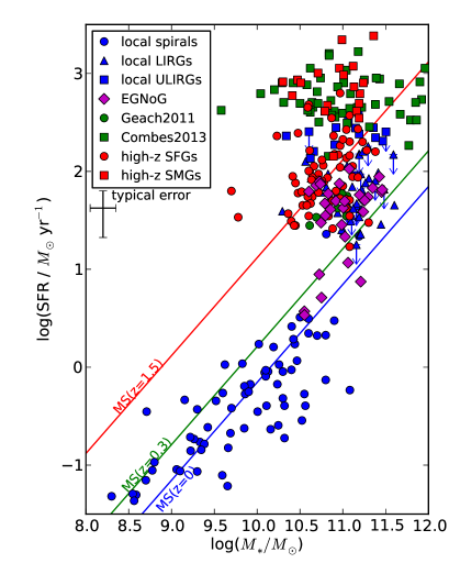
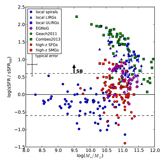
Figure 11.— Star formation rate (left panel) and normalized specific star formation rate (right panel) versus stellar mass for our literature sample and the EGNoG galaxies. Colors indicate approximate redshifts and plotting symbols show the galaxy type (see text for full description). In the left panel, the main sequence at three representative redshifts is indicated by the blue, green and red lines. In the right panel, the sSFR is normalized by the main sequence sSFR (for the relevant $z$ and $M_{*}$). Starburst (SB) galaxies lie above the higher dashed line.

While we have attempted to make this compilation of literature data as uniform as possible, the derived properties are not all calculated in a consistent fashion. In converting CO luminosities to molecular gas masses, we have standardized the selection of $\alpha_{\mathrm{CO}}$ value using the starburst classification of Equations 1 and 2 (described in the next section). The $J_{\mathrm{upper}}>1$ CO luminosities are converted to CO($J=1\rightarrow 0$) luminosities using the ratios prescribed by the individual authors in the case of ULIRGs and SMGs. We use standard ratios for all other galaxies: $r_{31}=0.5$ and $r_{21}=0.8$. The $M_{*}$ and SFR values, however, are calculated by a variety of methods, as described above. This may have systematic effects on the analysis in the following sections. In the interest of comparing with as large a sample as possible, we include all the data described here in our analysis, but note that systematic effects may be present.

5.2. Identifying Starburst Galaxies

In Figure 11, we present the stellar mass and star formation properties of the literature sample and the EGNoG survey galaxies. For the literature sample, the colors indicate approximate redshifts ($z\approx 0$ in blue, $z\sim 0.05-0.5$ in green, and $z>1$ in red) and the symbols indicate galaxy type: normal galaxies (local spirals, Geach et al., 2011 galaxies at $z=0.4$ and high-redshift SFGs) are marked with circles, local LIRGs with triangles, and starbursts (local ULIRGs, Combes et al. intermediate-redshift ULIRGs, and high-redshift SMGs) are marked with squares. The EGNoG galaxies are plotted with a unique symbol and color (magenta diamond) for emphasis. This color and symbol scheme will be used for the rest of this work.

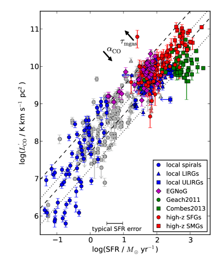
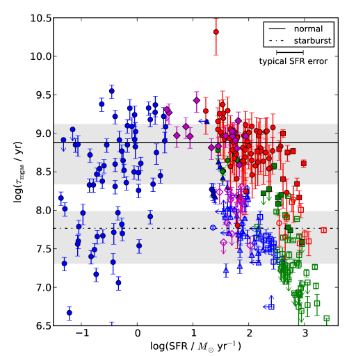
Figure 12.— CO luminosity ($L_{\mathrm{CO}}^{\prime}$; left panel) and molecular gas depletion time ($\tau_{\mathrm{mgas}}$; right panel) versus SFR. In the left panel, galaxies from Yao et al. (2003), Mao et al. (2010), and Papadopoulos et al. (2012) are plotted (gray points) in addition to the literature sample. Dashed (dotted) lines show the expected region in $L_{\mathrm{CO}}^{\prime}$-SFR space occupied by normal (starburst) galaxies. In the right panel, the horizontal solid (dot-dashed) line indicates the average $\tau_{\mathrm{mgas}}$ value for normal (starburst) galaxies, the gray region indicating $\pm 1\sigma$. Starburst galaxies are plotted as un-filled symbols in the right panel.

The left panel of Figure 11 shows the SFR versus $M_{*}$, with the main sequence at three representative redshifts indicated by the blue ($z=0$), green ($z=0.3$), and red ($z=1.5$) lines. Normal galaxies lie near the main sequence curve at the corresponding redshift. In order to more precisely discern starburst galaxies from normal galaxies, in the right panel of Figure 11 we plot the sSFR of each galaxy normalized by the main sequence sSFR (sSFR_MS; Equation 1) at the redshift and stellar mass of the galaxy. The horizontal black line indicates the main sequence relation, with the dashed lines showing a spread of 0.6 dex. Starburst galaxies lie above the higher dashed line, with sSFRs larger than 4 times the main sequence sSFR (as defined in Equation 2). In most cases, our starburst classification agrees well with expectations (e.g. ULIRGs are mostly classified as starbursts), with the exception of the SMG population, which we find to be mostly consistent with the main sequence defined in Equations 1 and 2. However, we note that since most of the SMGs included here are at $z\gtrsim 2$, this result depends sensitively on the high-redshift behavior of the sSFR${}_{\mathrm{MS}}(z)$ prescription, which is more uncertain and may flatten at these redshifts (see discussion in Section 2.1).

Using this starburst criterion, we standardize the conversion of CO luminosity to molecular gas mass in our literature sample, as we did for the EGNoG galaxies in Section 4.1. For galaxies that are classified as starburst based on their specific star formation rates, we use the value observed in starburst systems: $\alpha_{\mathrm{CO}}(\mathrm{ULIRG})=0.8$ M_⊙ (K km s^-1 pc²)^-1 (local ULIRGs: Scoville et al. 1997, Downes & Solomon 1998; high-redshift SMGs: Tacconi et al. 2008). For all other galaxies, we use a Milky Way-like conversion factor, $\alpha_{\mathrm{CO}}(\mathrm{MilkyWay})=3.2$ M_⊙ (K km s^-1 pc²)^-1 (e.g. Dame et al., 2001). These conversion factors do not explicitly include He; see Equation 4. This bimodal prescription for the conversion factor is discussed further in Section 5.5.

5.3. Gas Depletion Time

Using our compilation of data, we investigate the molecular gas depletion time ($\tau_{\mathrm{mgas}}$) for starburst and normal galaxies. Excluding dwarf galaxies, the average molecular gas depletion time for the normal (non-starburst) galaxies is $0.76\pm 0.54$ Gyr. The average for the starburst galaxies is $0.06\pm 0.04$ Gyr. (In calculating these averages, we have excluded galaxy Q2343-MD59 from Tacconi et al., 2012, as it is an obvious outlier.) These averages generally agree with previous work (see references for the literature sample in Section 5.1). However, we note that a depletion time calculated from molecular gas and SFR surface densities may differ from ours (calculated from the total molecular gas mass and SFR) due to different scale lengths of the CO and SFR distributions and trends in gas depletion time with galaxy size (larger galaxies will dominate an area-weighted average gas depletion time). This is the case for the sample of Leroy et al. (2008), in which the authors calculate an average molecular gas depletion time of 1.9 Gyr using surface densities, while the average depletion time using total quantities would be 1.3 Gyr (which lies within the error of our average value for normal galaxies).

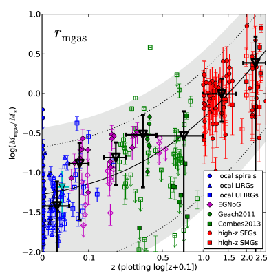
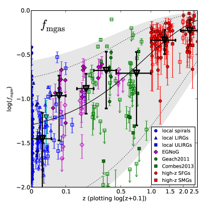
Figure 13.— Molecular gas ratio ($r_{\mathrm{mgas}}$) and molecular gas fraction ($f_{\mathrm{mgas}}$) versus redshift. We plot $log(z+0.1)$ on the x-axis. The average value from the COLDGASS survey is plotted as a cyan upside-down triangle. Starburst galaxies are plotted as un-filled symbols. Average values (with $1\sigma$ errors) for each of 6 redshift bins are plotted as un-filled black upside-down triangles. The shaded gray area shows the expected behavior for normal galaxies, with the solid black curve indicating the average. The dotted black lines bound the expected behavior for starburst galaxies.

In the left panel of Figure 12, we plot CO luminosity versus SFR to illustrate that starburst and normal galaxies fill the same space in this plane, making the differentiation of starburst from normal galaxies impossible using only CO luminosity and SFR. In addition to the literature sample described in Section 5.1, we include here local spirals, LIRGs and ULIRGs from Yao et al. (2003), Mao et al. (2010) and Papadopoulos et al. (2012) as gray circles, triangles and squares respectively. These datasets do not include stellar masses and thus are only included in this plot for illustrative purposes (we estimate SFRs from the far-IR luminosities using the Kennicutt 1998b conversion). The dashed lines indicate the area of the plane occupied by normal galaxies using $\alpha_{\mathrm{CO}}(\mathrm{MilkyWay})$ and the average $\tau_{\mathrm{mgas}}$ for normal galaxies given above. The dotted lines indicate the area occupied by starburst galaxies (using $\alpha_{\mathrm{CO}}(\mathrm{ULIRG})$ and the starburst $\tau_{\mathrm{mgas}}$), which overlaps the normal galaxy area significantly. This overlap occurs because the differences in $\alpha_{\mathrm{CO}}$ and $\tau_{\mathrm{mgas}}$ between starburst and normal galaxies cancel each other out in this plane: as the effective $\alpha_{\mathrm{CO}}$ increases, a galaxy moves toward the lower right and as the effective $\tau_{\mathrm{mgas}}$ increases, a galaxy moves toward the upper left.

In the right panel of Figure 12, the molecular gas depletion time is plotted against SFR, with the average value for normal (starburst) galaxies indicated by the solid (dot-dashed) line. 1$\sigma$ error bars on the averages are indicated by the gray shaded regions. The CO to H₂ conversion factor used for each data point is indicated by the fill of the symbol: filled symbols are normal ($\alpha_{\mathrm{CO}}($Milky Way$)$) and un-filled symbols are starburst ($\alpha_{\mathrm{CO}}($ULIRG$)$) according to the sSFR criterion in Equation 2 (plotted in the right panel of 11. Only galaxies that can be classified this way (galaxies for which the $M_{*}$ and SFR have been estimated) are included in this plot. Note that the $\tau_{\mathrm{mgas}}$ error bars plotted only represent the error associated with the CO measurement and not the SFR error since we do not have errors on all the SFR measurements in the literature sample. We estimate that the typical SFR error is $\pm 50\%$.

The population of non-starbursting, local galaxies in the lower left corner of the right panel are dwarfs ($M_{*}<10^{10}$), for which a larger conversion factor may be more appropriate due to decreasing metallicity. Leroy et al. (2011) find that the conversion factor begins to increase significantly as the metallicity falls below $12+\log(\mathrm{O}/\mathrm{H})=8.2-8.4$, which is expected for $M_{*}\lesssim 10^{9}$ M_⊙ (Tremonti et al., 2004). This change in conversion factor would shift the dwarf galaxy points to higher $\tau_{\mathrm{mgas}}$. Therefore, we do not include dwarf galaxies in the calculation of the average $\tau_{\mathrm{mgas}}$ values.

5.4. Evolution of the Molecular Gas Fraction

In order to calculate the expected evolution of the molecular gas fraction, we first consider the ratio of the molecular gas mass to the stellar mass ($r_{\mathrm{mgas}}$), which can be written as the product of the molecular gas depletion time and the specific star formation rate:

$$r_{\mathrm{mgas}}=\frac{M_{\mathrm{mgas}}}{M_{*}}=\frac{M_{\mathrm{mgas}}}{\mathrm{SFR}}\frac{\mathrm{SFR}}{M_{*}}=\tau_{\mathrm{mgas}}\times\mathrm{sSFR}$$ (7)

In Section 2.1, we motivated and defined the sSFR of the main sequence as a function of redshift and stellar mass. As illustrated in the right panel of Figure 11, main sequence galaxies lie roughly within a factor of 4 ($\pm 0.6$ dex) of the main sequence relation and starburst galaxies lie at sSFRs 4 to 30 times larger than the main sequence value. In the previous section, we found an average $\tau_{\mathrm{mgas}}$ of $0.76\pm 0.54$ Gyr for normal galaxies and $0.06\pm 0.04$ Gyr for starburst galaxies. Using these typical $\tau_{\mathrm{mgas}}$ values and sSFR ranges (relative to the sSFR_MS; see Equation 1), we get:

$$r_{\mathrm{mgas}}(\mathrm{normal})=\\ (0.05\pm 0.04)\eta_{\mathrm{norm}}(1+z)^{3.2}M_{*,11}^{-0.2}$$ (8)

$$r_{\mathrm{mgas}}(\mathrm{starburst})=\\ (0.04\pm 0.03)\left(\frac{\eta_{\mathrm{SB}}}{10}\right)(1+z)^{3.2}M_{*,11}^{-0.2}$$ (9)

where $M_{*,11}=M_{*}/(10^{11}\ \mathrm{M}_{\odot})$ and $\eta_{\mathrm{norm}}$ and $\eta_{\mathrm{SB}}$ are the ranges of sSFR/sSFR_MS values appropriate for normal and starburst galaxies, respectively: $\eta_{\mathrm{norm}}=1/4$ to $4$ and $\eta_{\mathrm{SB}}=4$ to $30$. In each of Equations 8 and 9, the scatter in $\tau_{\mathrm{mgas}}$ is reflected in the error of the first term ($\pm 0.04$ and $\pm 0.03$). The corresponding molecular gas fraction may be calculated from $r_{\mathrm{mgas}}$: $f_{\mathrm{mgas}}=(1+r^{-1}_{\mathrm{mgas}})^{-1}$. The result is that the expected behavior of $r_{\mathrm{mgas}}$ and $f_{\mathrm{mgas}}$ is remarkably similar for normal and starburst galaxies.

Figure 13 shows the data and expectation for $r_{\mathrm{mgas}}$ (left panel) and $f_{\mathrm{mgas}}$ (right panel) versus redshift, plotting $log(z+0.1)$ on the x-axis in order to spread out the low to intermediate redshifts for clarity. As in the right panel of Figure 12, the starburst galaxies (identified using Equation 2) are plotted as un-filled symbols. Note that the error bars plotted only represent the error associated with the CO measurement (and not the stellar mass error), since we do not have errors on all the stellar mass measurements in the literature sample. We estimate that a typical stellar mass error is 0.1-0.2 dex. We also plot the average value at $z=0.025-0.05$ reported by the COLDGASS survey (Saintonge et al., 2011) as a cyan upside-down triangle. We plot the expected $r_{\mathrm{mgas}}$ and $f_{\mathrm{mgas}}$ versus redshift for normal galaxies (Equation 8) as the solid black curve, with the gray shaded area indicating the range of possible values (we take a nominal $M_{*}$ of $10^{11}$ M_⊙). The range for starburst galaxies (Equation 9), indicated by the dotted black curves, overlaps the expected range for normal galaxies.

The data points are binned into 7 redshift ranges (number of detected galaxies in parenthesis): $z=0-0.05$ (110), $0.05-0.1$ (19), $0.15-0.25$ (18), $0.25-0.45$ (18), $0.45-1.0$ (15), $1.0-1.7$ (53), and $1.9-2.7$ (28). The average values (for all detections) are plotted as un-filled black upside-down triangles, with vertical lines showing the standard deviations (for the $z=0.25-0.45$ bin, the obvious outlier from Combes et al., 2011 at $r_{\mathrm{mgas}}=3.8$ is excluded). All redshift bin averages lie within the expected range for both normal (gray shaded region) and starburst (dotted lines) galaxies, and the average expectation curve ($r_{\mathrm{mgas}}=\mathrm{sSFR}_{\mathrm{MS}}\times(0.76$ Gyr)) lies within the dispersion (vertical black lines).

We note that the three intermediate redshift bins ($z=0.05-0.01$, $0.15-0.25$, and $0.25-0.45$) lie systematically higher than the average expectation curve. However, the number of galaxies in each of these bins is small and is dominated by SFGs (EGNoG and Geach et al. galaxies), which we have shown to lie close to the starburst cutoff (see Figure 11). Therefore, these points are sensitive to the exact starburst criterion used (which determines $\alpha_{\mathrm{CO}}$). For example, if we consider galaxies with sSFR $>2$ sSFR_MS to be starbursts, the three intermediate redshift bin average values decrease by $\approx 0.2$ dex, falling more in line with the average expectation curve.

In summary, while the EGNoG galaxy redshift bins lie systematically higher than the average expectation curve for the starburst criterion (and resulting $\alpha_{\mathrm{CO}}$ choices) adopted in this work, a reasonable variation of this criterion results in a decrease of $\approx 0.2$ dex, bringing the averages in line with expectation. We also note, but do not investigate, that systematic effects may be present due to the use of different methods for calculating $M_{*}$ and SFR, and from instrumental sensitivity limiting CO detections to gas-rich galaxies at intermediate and high redshift. Overall, we conclude that the data agree well with the behavior of $r_{\mathrm{mgas}}$ and $f_{\mathrm{mgas}}$ expected from a simple prescription of sSFR and $\tau_{\mathrm{mgas}}$ with $z$ and $M_{*}$ in star-forming galaxies. While the EGNoG bin D galaxies (non-detections) have not been included in the redshift bin averages discussed above, we note that the four upper limits are included in Figure 13 and agree with expectations as well.

5.5. A Bimodal Conversion Factor Prescription

In this work, we have used a bimodal prescription for the conversion factor $\alpha_{\mathrm{CO}}$ in normal and starburst galaxies. We have included some local low-mass galaxies in our literature sample, but we do not include these systems in the calculation of average values since a different $\alpha_{\mathrm{CO}}$ is likely appropriate due to decreasing metallicity (Leroy et al., 2011; Narayanan et al., 2012). While our bimodal prescription (excluding low-mass galaxies) likely does not describe the true conversion factor in all of these galaxies (e.g. simulations by Narayanan et al. 2012 suggest a continuous variation of $\alpha_{\mathrm{CO}}$ from normal to starburst galaxies), it appears to capture the typical behavior. A recent study by Magnelli et al. (2012) using observed dust masses to calculate the conversion factor in $z>1$ star-forming galaxies found smaller conversion factors in starburst galaxies (classified by sSFR, as in this work), but it was unable to distinguish between a step function and a continuous variation of $\alpha_{\mathrm{CO}}$ as a function of sSFR/sSFR_MS. In this work, we have used only total measurements of the galaxy properties, and we note that with resolved CO measurements, it would be possible to apply a value of $\alpha_{\mathrm{CO}}$ more tailored to local conditions (like the prescriptions of Narayanan et al., 2012; Bolatto et al., 2013), which could tighten the observed relations.

Independent of this issue of bimodal or continuous conversion factor is the question of whether the local values for normal and starburst conversion factors may be extended to high redshift. Both simulations by Narayanan et al. (2012) and observations by Daddi et al. (2010) suggest that the conversion factor is lower than the Milky Way value in normal star-forming galaxies at high redshift. We cannot answer this question with the current dataset, but note that using a reduced $\alpha_{\mathrm{CO}}$ in high-redshift SFGs or a continuous variation of $\alpha_{\mathrm{CO}}$ from normal to starburst galaxies would not change the general conclusions.

6. Conclusions

In this paper, we present the EGNoG survey: CO observations of 31 galaxies from $z=0.05$ to $z=0.5$. We detect 24 of the 31 observed galaxies, providing integrated CO maps, spectra, and luminosities for detections and $3\sigma$ upper limits for non-detections.

We place the EGNoG galaxies in context with a sample of 185 normal and starburst galaxies at low and high redshift collected from the literature. We standardize the comparison of the EGNoG and literature galaxies using a simple prescription for molecular gas mass calculation. Each galaxy is classified as normal or starburst based on its sSFR relative to the sSFR of the main sequence of star-forming galaxies at that redshift and stellar mass (see Equations 1 and 2). We then use a bimodal prescription for $\alpha_{\mathrm{CO}}$ based on this classification (a Milky Way-like value for normal galaxies, a ULIRG-like value for starbursts), and calculate the molecular gas mass, molecular gas depletion time, and molecular gas fraction of each galaxy.

Using this prescription, we find an average molecular gas depletion time of $0.76\pm 0.54$ Gyr for normal galaxies and $0.06\pm 0.04$ Gyr for starburst galaxies. We calculate an average molecular gas fraction of 10-20% at the intermediate redshifts probed by the EGNoG survey ($z=0.05-0.5$). By expressing the molecular gas fraction in terms of the sSFR and molecular gas depletion time ($f_{\mathrm{mgas}}=(1+[\tau_{\mathrm{mgas}}\times\mathrm{sSFR}]^{-1})^{-1}$), and using typical ranges of sSFR and $\tau_{\mathrm{mgas}}$ for starburst and normal galaxies, we calculate the expected evolution of the molecular gas fraction with redshift. We find that the expected behavior for normal and starburst galaxies is remarkably similar and agrees well with the EGNoG and literature data from $z=0$ out to $z\sim 2.5$.

——————————————————————-

Appendix A Stellar Mass and SFR Probability Distribution Functions

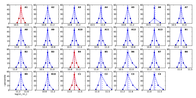
Figure 14.— Stellar mass (top) and SFR (bottom) probability distribution functions of EGNoG galaxies selected from SDSS (bins A, B and C). For galaxies A1, B4 and C1, a duplicate SDSS source exists, over-plotted in red.

For each of the EGNoG galaxies in redshift bins A-C, we show the stellar mass and SFR probability distribution functions in Figure 14 in the top and bottom panels respectively. These distributions come from the MPA-JHU group (see text) for SDSS DR7 galaxies. Data points give the 2.5, 16, 50, 84 and 97.5 percentiles of the distribution. The median, mean and mode are indicated by the vertical solid, dashed and dotted lines respectively. For galaxies A1, B4 and C1, a duplicate SDSS source exists (as a result of SDSS automated source-finding). The duplicate source is plotted in red in Figure 14. For each of the quantities plotted in Figure 14 (stellar mass in the top panels, SFR in the bottom panels), the x-axis range is constant.

Appendix B Data Reduction and Flux Measurement

Calibrator	Obs.	Freq.		Flux	Primary Calibrator
Name	Band	(GHz)	Date Range	(Jy)	(Flux in Jy)
0006–063	3mm	105	Oct 2010	1.6	MWC349 (1.28 Jy)
0010+109	3mm	109	Nov 2010	0.2	Uranus
0108+015	3mm	97	Sep 2011	2.0	Uranus; Neptune
0108+015	3mm	97	Feb 2012	1.7	Uranus
0854+201p	3mm	107	Nov 2010	5.2	3C84 (11 Jy)
0854+201p	3mm	98	Aug-Oct 2011	4.0	Mars
0854+201p	3mm	98	Nov 2011	5.2	Mars
0854+201p	3mm	98	Feb 2012	5.2	Mars
0854+201	1mm	258	Aug 2011	2.0	Mars
0854+201	1mm	254	Apr 2012	4.0	Mars
0920+446	3mm	106	Nov 2010	1.9	3C84 (11 Jy)
0920+446	3mm	106	Feb 2012	1.0	3C84 (15 Jy)
0958+655	3mm	105	Nov 2010	1.1	3C273 (12 Jy)
0958+655	3mm	105	Feb 2012	1.7	MWC349 (1.28 Jy)
1058+015p	3mm	107	May 2011	4.6	3C84 (10 Jy)
1058+015p	3mm	99	Nov 2011	4.1	Mars
1058+015p	3mm	99	Feb 2012	3.6	Mars
1058+015p	3mm	99	Apr 2012	2.8	Mars
1058+015	1mm	266	Aug 2011	2.6	Mars
1058+015	1mm	226	Apr 2012	2.0	Mars
1159+292	3mm	105	Apr-May 2011	1.4	3C84 (10 Jy); 3C273 (10 Jy)
1159+292	3mm	105	Feb 2012	0.7	Mars
1224+213	1mm	252	Apr 2012	0.6	Mars
1310+323	3mm	90	Sep-Nov 2011	1.7	Mars
1310+323	3mm	98	Apr 2012	1.4	Mars
1310+323	1mm	266	Aug 2011	0.6	MWC349 (2.0 Jy)
1357+193	3mm	105	Apr-May 2011	0.7	MWC349 (1.28 Jy)
1357+193	3mm	105	Sep-Nov 2011	0.8	Mars; MWC349 (1.28 Jy)
2134–018	3mm	106	Apr 2011	1.2	Uranus
2232+117	3mm	106	Apr 2011	1.3	MWC349 (1.28 Jy)
2232+117	3mm	97	Aug-Sep 2011	1.5	Uranus; MWC349 (1.23 Jy)
2232+117	3mm	97	Feb 2012	1.7	Uranus; Neptune; MWC349 (1.23 Jy)
3C273	3mm	98	Apr 2012	6.8	Mars
3C454.3	3mm	107	Oct 2010	39.5	Uranus

Table 5Summary of calibrator fluxes used to set the flux scale of EGNoG data. For each flux, the observing band (1 or 3 mm), frequency, and date range are listed. The last column lists the primary calibrator used to set the flux. For non-planet calibrators, the flux used (at the frequency given in the third column) is given in parentheses.
^p Indicates the calibrator is linearly polarized, requiring additional reduction steps (only applicable for 3 mm data) detailed in Appendix C.

B.1. Data Reduction

Each dataset was reduced and calibrated as follows. The data were flagged for antenna - antenna shadowing and any other issues present during the observation (e.g. high system temperature, high gain, tracking problem, etc.). The instrument bandpass was calibrated with mfcal on a bright passband calibrator. The time-dependent antenna gains (from atmospheric variation) were derived by performing a selfcal on the phase calibrator with an averaging interval of 18 minutes (the timescale of switching between the source and phase calibrator). For galaxies A5, A11, B3, B4, B7, C1 and C2, the phase calibrator (0854+201 or 1058+015) was up to 10% polarized, which required additional steps in the reduction of the 3mm data (observed with linearly polarized feeds). This is described in detail in Appendix C.

For each dataset, the flux of the phase calibrator was set during the antenna gain calibration in order to properly set the flux scale of the data. The flux of each phase calibrator was assumed to be constant over timescales of weeks, and was therefore determined from the best datasets of the survey using bootflux on bandpass-calibrated, phase-only gain-calibrated data using a planet (Uranus, Neptune or Mars) or MWC349 as a primary flux calibrator. In some cases, none of these flux calibrators was available so a bright quasar (3C84 or 3C273) was used instead, with the flux estimated using historical flux monitoring data at CARMA. Table 5 provides the flux used for each phase calibrator and the primary calibrator used. For non-planet primary calibrators, the flux used is given in parenthesis. The flux of MWC349 was calculated assuming 1.2 Jy at 92 GHz with a spectral index of 0.5, the typical value from historical flux monitoring at CARMA^,. The brightness temperature ($T_{b}$) of the planets was set by the CARMA system. The brightness temperature of Mars comes from the Caltech thermal model of Mars (courtesy of Mark Gurwell), which includes seasonal variations in temperature. This model can be accessed in MIRIAD using marstb. For Uranus and Neptune, the CARMA system uses the following power laws:

$$T_{b}(\mathrm{Uranus})=134.7\left(\frac{\nu}{\mathrm{100~{}GHz}}\right)^{-0.337}~{}\mathrm{K}$$ (B1)

$$T_{b}(\mathrm{Neptune})=129.8\left(\frac{\nu}{\mathrm{100~{}GHz}}\right)^{-0.350}~{}\mathrm{K}$$ (B2)

Data cubes were produced combining all fully calibrated datasets of each source. We used invert, weighting the visibilities by the system temperature as well as using a Briggs’ visibility weighting robustness parameter (Briggs, 1995) of 0.5. Since CARMA is an inhomogeneous array (these data use both the 10 and 6 m dishes), we also use options=mosaic in the invert step to properly handle the three different primary beams patterns (10m-10m, 10m-6m and 6m-6m). All observations consisted of a single pointing. The resulting cubes are primary-beam-corrected. If channel averaging was required (based on the strength of the CO line), this was done in the invert step.

We deconvolved each image with mossdi (the mosaic version of clean), cleaning down to the rms noise within a single channel, within a cleaning box selected by eye to include only source emission. We cleaned only channels containing visible source emission. Cleaning down to a specified noise level is preferred to using a set number of clean iterations due to the nature of the spectral line emission: some channels will contain more flux and therefore require more clean iterations. In tests using a model source of known flux inserted into real data (emission-free channels), we found a $1\sigma$ cutoff to best extract the true source emission without overestimating the flux over a range of detection significance levels, with a 10-30% uncertainty in the recovered flux (depending on the significance of the signal). The final cleaned cubes were produced by restor, which convolves the clean component cube with a clean beam (calculated by fitting a Gaussian to the combined mosaic beam given by mospsf) and adds the residuals from the cleaning process.

B.2. Flux Estimation

Total source fluxes in the CO lines are calculated by summing ‘source’ pixels in each ‘source’ velocity plane of the final, calibrated, cleaned cubes. The source velocity planes are selected by eye. The source pixels are those within the ‘source’ region which are not masked by our smooth mask, adapted from the masked moment method of Dame (2011). The smooth mask is created by applying a $2\sigma$ clip to a smoothed version of the image: Hanning smoothing is done along the velocity axis, and each velocity plane is convolved spatially with a Gaussian beam twice the size of the original synthesized beam. This smoothed mask is used to exclude noise pixels but still capture low-level emission that a simple $\sigma$-clip (without smoothing) would miss. In our own testing (using a model source of known flux inserted into real data), we found a $2\sigma$ clip to best reproduce the true flux over a range of detection significance levels.

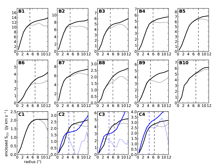
Figure 15.— Enclosed flux versus radius for bin B and C sources. The masked (unmasked) data are shown by the solid (dotted) line. The vertical dashed line indicates the source region radius adopted for each galaxy. For galaxies C2, C3 and C4, the CO($J=1\rightarrow 0$) line data are shown in black and the CO($J=3\rightarrow 2$) line data in blue.

An appropriate source region size was selected to recover all of the flux without including the negative bowl. Since we do not have single-dish data to complement the interferometric data presented here, our datasets are missing the shortest $uv$ spacings. As a result, the emission in the clean maps sits in a negative bowl, which will affect the measured flux (calculated by summing pixels within a given radius). The bin A galaxies are observed with a sufficiently small beam so that the galaxies are resolved. In this case, we use an elliptical source region selected by eye to enclose the spatial extent of the CO emission of each galaxy. In the case of the bins B and C galaxies, the molecular gas is unresolved, so we use a circular source region with radius set to the radius at which the radial profile of the enclosed flux first peaks, thereby excluding the negative bowl. The radial profiles of the enclosed flux for bin B and C sources are shown in Figure 15. The negative bowl is most evident in the unmasked profiles (dotted lines in Figure 15), in which the enclosed flux peaks and then decreases with radius. We have selected the following source region radii by eye (approximately the radius at which the enclosed flux first peaks): $4.5\arcsec$ for bin C sources in the CO($J=3\rightarrow 2$) line (1 mm data); $5\arcsec$ for sources B1, B2, B3, B7 and B9; $6\arcsec$ for B4 and B8; $6.5\arcsec$ for bin C sources in the CO($J=1\rightarrow 0$) line (3 mm data); $7\arcsec$ for B6 and B10; $8\arcsec$ for B5. The source region radius of each galaxy in bins B and C is indicated by the vertical dashed line in each panel of Figure 15. For all galaxies, the source region is indicated by the dotted white ellipse in the moment 0 and moment 1 maps of Figures 3 - 8.

The error in each flux measurement is estimated from the standard deviation of the measured fluxes using different velocity channel averaging and starting channels, using three different methods of calculating the flux in each case. The three methods are: the $2\sigma$ masking technique described above, the same masking technique with a $3\sigma$ clip, and the simple addition of all pixels (no mask) within the source region.

We performed extensive testing of our analysis technique to choose the parameters of the reduction to eliminate systematic offsets and minimize the uncertainty due to noise (as described above). We find a 10-30% error in the flux measurement in each channel coming from noise in the data and the adopted reduction and analysis steps. From this, we adopt an average uncertainty of 20% in the flux estimated in each channel, which results in an uncertainty in the total flux of 20%$N_{\mathrm{ch}}^{-0.5}$, where $N_{\mathrm{ch}}$ is the number of velocity channels in which the flux is summed. For the total flux values reported in Table 3, we estimated the errors from the variations in the fluxes calculated using different channel averaging, flux measurement methods, etc. (as described above), consistent with the 20%$(N_{\mathrm{ch}})^{-0.5}$ expected.

Further, these data suffer from systematic effects due to the absolute flux calibration and primary beam correction. We set the flux scale in our dataset using a primary flux calibrator, the flux of which is only known to $\approx 20\%$. In the primary beam correction of the dataset, pointing and focus errors at the time of the observations as well as errors in the primary beam model can significantly reduce image fidelity, leading to errors in the measured fluxes of $\approx 20\%$ (see Square Kilometer Array (SKA) Memo #103, Wright & Corder 2008). Combining these errors in quadrature, we estimate that our flux measurements suffer from additional uncertainties of up to $\approx 30\%$. We consider all these factors in the presentation of our data in Table 3: for the line flux ($S_{\mathrm{CO}}$), we report the measured error; for $L_{\mathrm{CO}}^{\prime}$, we include an additional $30\%$ error (added in quadrature to the measured error in $S_{\mathrm{CO}}$).

Appendix C Polarized Calibrators

In this section, we describe how we calibrated datasets which used a strongly polarized source for gain calibration. This applies to the 3mm data only, which were taken using single-polarization, linearly polarized receivers. The 1mm data used dual-polarization, circularly polarized feeds and are thus not affected by the strong linear polarization present in some calibrators.

For Stokes I intensity $I$, linear polarization fraction $p_{qu}$, and polarization angle $PA$, the observed YY intensity as a function of parallactic angle $\chi$ is described by

$$YY=I\{1-p_{qu}\cos[2(PA-\chi)]\}$$ (C1)

Thus, the observed YY amplitude varies sinusoidally with parallactic angle in a dataset. Any amplitude self-calibration on the gain calibrator would assume constant amplitude with time and yield higher or lower gains according to this amplitude variation. Since this effect can be as large as 10% in some cases, we corrected for it in the following way. After a phase-only selfcal, we used a modified version of uvcal to remove the known polarization effect from the calibrator data and then performed an amplitude selfcal. The resulting gains should represent the atmospheric variations during the track, with the influence of the polarization of the calibrator removed.

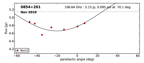
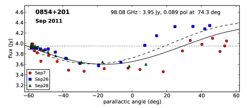
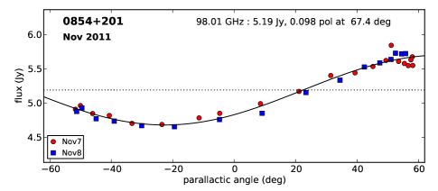
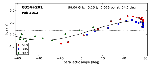
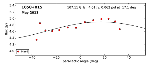
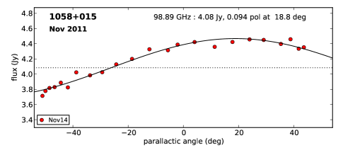
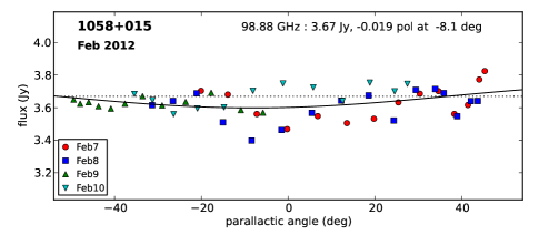
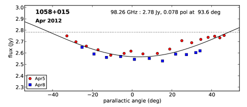
Figure 16.— Polarization of calibrators 0854+201 (left) and 1058+015 (right). In each panel, flux versus parallactic angle is plotted for the best datasets at each epoch (indicated in the upper left). The solid black line shows the best fit, with the dotted black line indicating the best-fit Stokes I flux. Calibrator 0854+201 (left) was observed at four epochs: at 107 GHz in November 2010 and at 98 GHz in September 2011, November 2011 and February 2012. Calibrator 1058+015 (right) was observed at four epochs as well: at 107 GHz in May 2011 and at 99 GHz November 2011, February 2012 and April 2012.

This procedure was used for two calibrators: 0854+201 and 1058+015. We do not assume stability over long timescales in the polarization parameters of the calibrators (and in fact find evidence for significant variation with time), so the polarization parameters for each source are derived in each epoch from the best datasets. The flux scale in most of the datasets was calibrated using Mars, with brightness temperatures from the Caltech thermal model by Mark Gurwell, which includes seasonal variations. Datasets from November 2010 and May 2011 use 3C84 as the flux calibrator. Based on flux monitoring at CARMA, we assumed a flux of 11 Jy in November 2010 and 10 Jy in May 2011 (both at 107 GHz).

Calibrator	Epoch	$\nu_{\mathrm{obs}}$	Stokes I	$p_{\mathrm{qu}}$	Angle
		(GHz)	Flux (Jy)		(deg)
0854+201	Nov 2010	106.6	5.2	0.10	70
	Sep 2011	98.1	4.0	0.10	67
	Nov 2011	98.0	5.2	0.10	67
	Feb 2012	98.0	5.2	0.08	54
1058+015	May 2011	107.0	4.6	0.08	19
	Nov 2011	98.9	4.1	0.09	19
	Feb 2012	98.9	3.6	-	-
	Apr 2012	98.3	2.8	0.08	94

Table 6Polarized calibrator parameters. The values given in the table are those that were used in the reduction of the relevant datasets. In some cases, these are not the same as the best fit values. See text for discussion.

The fits in the different epochs are shown in Figure 16, with 0854+201 on the left and 1058+015 on the right. Flux versus parallactic angle is plotted, with data points for each dataset marked with a different symbol (indicated in the legend) and the best fit line (Equation C1) in solid black. The dotted black line shows the best fit Stokes I flux. The observing frequency and best-fit parameters are given in the upper right corner of each panel. The polarization parameters used for each calibrator, in each epoch, are given in Table 6.

While the fit for 0854+201 in November 2010 is not well constrained due to limited parallactic angle coverage, it agrees with subsequent epochs, so we use it. The fit for 0854+201 in September 2011 is not very good due to noisy data, but the good fit from November 2011 (scaled to the average flux in September 2011; black dashed line) appears to match the September 2011 data well. Therefore, we use the November 2011 polarization fraction and angle for September 2011, with an average Stokes I flux of 4.0 Jy.

The data for 1058+015 from November 2011 to April 2012 suggest a radical change in polarization, from 9% polarized at 19 degrees to 8% polarized at 94 degrees over the course of 6 months. The data from February 2012 show no indication of polarization (in fact, the best fit is a negative polarization fraction). This disappearance and (rotated) reappearance of the linear polarization component of 1058+015 is coupled with a significant decrease in flux.

Appendix D $uv$-Spectra

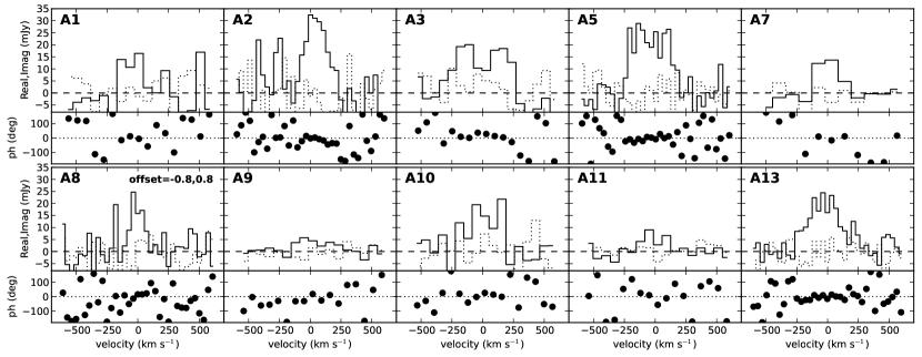
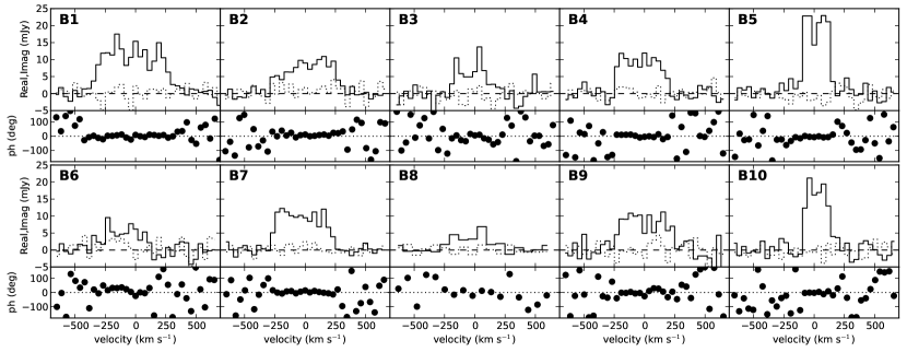
Figure 17.— $uv$-spectra of bin A and B galaxies. The top panel shows the vector-averaged Real (solid) and Imaginary (dotted) amplitudes (Real,Imag in mJy beam^-1) and the bottom panel shows phase (ph, degrees) of the calibrated $uv$ data versus velocity (km s^-1). For galaxy A8, the spectrum is calculated at a $-0.8\arcsec,0.8\arcsec$ offset from the SDSS position (indicated in the upper right corner of the A8 panel).

We show the $uv$-spectra for all detected galaxies in Figures 17 and 18. For each galaxy (indicated in the top left), the top (bottom) panel shows the vector-averaged Real and Imaginary amplitudes (phase) of the calibrated $uv$ data versus velocity. In Figure 18, the CO($J=1\rightarrow 0$) line is shown in the top panels and the CO($J=3\rightarrow 2$) line in the bottom panels. For galaxy A8 and the CO($J=3\rightarrow 2$) line in galaxies C1 and C2, the spectrum is calculated at a position offset from the SDSS position in order to coincide with the observed peak of the CO emission. For a compact source at the center of the field of view, the Real part shows the signal without a noise bias, and the Imaginary part shows the noise. In all cases (except CO($J=3\rightarrow 2$) in galaxy C1), we see coherent emission (larger Real amplitudes coincident with noise-like Imaginary amplitudes and phases of $\approx 0^{\circ}$) over multiple velocity channels, indicative of a detection. We do not detect the CO($J=3\rightarrow 2$) line in galaxy C1.

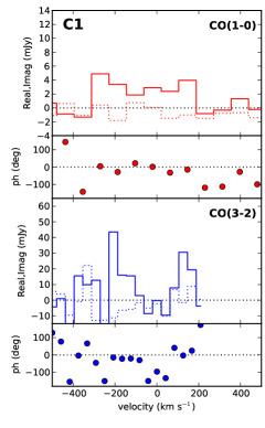
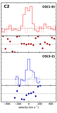
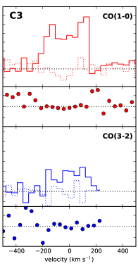
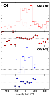
Figure 18.— $uv$-spectra of bin C galaxies. For each source, the top row (red) shows the CO($J=1\rightarrow 0$) line and the bottom row (blue) shows the CO($J=3\rightarrow 2$) line. For each line, for each source, the top panel shows the vector-averaged Real (solid) and Imaginary (dotted) amplitudes (Real,Imag in mJy beam^-1) and the bottom panel shows phase (ph, degrees) of the calibrated $uv$ data versus velocity (km s^-1). With the higher resolution of the CO($J=3\rightarrow 2$) data, we observe the peak of the CO($J=3\rightarrow 2$) emission to be offset ($<1.5\arcsec\sim 6$ kpc) from the centers of galaxies C1 and C2. In these cases, we calculate the $uv$ spectra at the peak of the CO($J=3\rightarrow 2$) emission. For the CO($J=1\rightarrow 0$) line of galaxy C1, we average 2 channels together in order to increase the signal to noise ratio.

Appendix E Extraordinary CO Emission in Galaxies A3 and A8

The integrated CO emission maps of galaxies A3 ($z=0.06$) and A8 ($z=0.10$) show evidence for disturbed morphologies. In both galaxies, we detect CO emission coincident with the optical emission, which shows a velocity gradient misaligned with respect to the optical major axis. In galaxy A8 we detect CO emission outside of the optical emission. Our observations are suggestive of CO emission outside the optical emission of A3 as well, but are not conclusive. In this Appendix, we investigate these emission components using $uv$-spectra calculated at various positions in the field to distinguish true emission from noise. We discuss the more compelling case of galaxy A8 first, then A3.

E.1. EGNoG A8

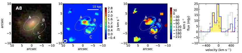
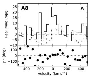
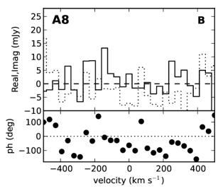
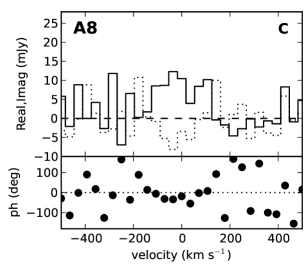
Figure 19.— Optical image, moment maps, integrated spectra and $uv$-spectra for EGNoG galaxy A8. The top four panels show (from left to right) the optical image, the moment 0 map, the moment 1 map and the integrated spectrum (as in Figure 3) of the main part of the galaxy (solid blue shows spectrum with masking, dotted green without). The integrated spectrum of the external CO component is also shown by a red dashed line. The bottom three panels show the $uv$-spectra (amplitude and phase) versus velocity of each of the 3 points (A,B and C) marked in the moment maps in the top row.

In Figure 19, we show the optical image, moment maps, integrated spectrum (as in Figure 3), and $uv$-spectra of galaxy A8. In the top right panel, the solid blue (green dotted) line shows the integrated spectrum with (without) masking of the main CO component, indicated by the central white dotted ellipse in the moment map panels. The dashed red line shows the integrated spectrum of the emission component outside the optical galaxy (the offset white dotted ellipse in the map panels). The bottom three panels show the $uv$-spectra (amplitude and phase versus velocity) at 3 points, A, B and C, labeled on the map panels in the top row.

Point A is centered on the CO emission coinciding with the optical emission. We only detect CO emission corresponding to the upper right (north-west) half of the optical galaxy, at negative velocities (relative to the optical redshift from SDSS). The moment 1 map (intensity-weighted velocity) of this component shows a velocity gradient suggestive of a rotating disk. However, this velocity gradient does not lie along the optical major axis, but appears to be rotated by 45 to 90 degrees.

Points B and C are at two positions along the long axis of the CO component that lies outside the optical galaxy (following the velocity gradient). The optical image from the SDSS shows no optical counterpart to this component of the CO emission. While the $uv$-spectrum at point B appears dominated by noise, point C shows phases of $\approx 0^{\circ}$ over several velocity channels, indicative of real emission. This CO component shows a velocity gradient parallel to the major axis of the optical galaxy and is therefore not aligned with the velocity gradient of the CO disk component. However, the two components become roughly spatially coincident at negative velocities.

In summary, the molecular gas in galaxy A8 is disturbed: CO emission is observed coinciding with the north-west half the optical galaxy but not in the south-east portion; the velocity gradient of the CO emission is not aligned with the optical major axis; and we observe significant CO emission outside the optical galaxy, with no optical counterpart. The optical image does not indicate interaction. We note that there is another galaxy in the field (seen on the left side of the optical image), but this galaxy is in the SDSS catalog with a photometric redshift of 0.28. The CO flux of component outside the disk is 3.2 Jy km s^-1, with $v_{\mathrm{center}}=-110$ km s^-1 and $\Delta V=357$ km s^-1. This is very similar to the main CO component: $S_{\mathrm{CO}}=4.5$ Jy km s^-1, with $v_{\mathrm{center}}=-67$ km s^-1 and $\Delta V=357$ km s^-1. If the emission outside of the optical disk traces dense molecular gas, the molecular gas mass of this component (assuming a Milky Way-like conversion factor) would be $6.5\times 10^{9}$ M_⊙, roughly 70% the molecular mass of the component coincident with the optical emission.

E.2. EGNoG A3

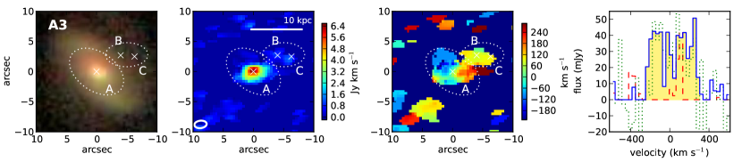
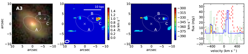
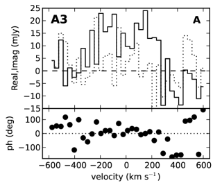
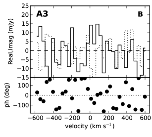
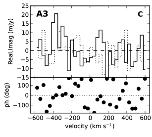
Figure 20.— Optical image, moment maps, integrated spectra and $uv$-spectra for EGNoG galaxy A3. The top four panels show (from left to right) the optical image, the moment 0 map, the moment 1 map and the integrated spectrum (as in Figure 3) of the main part of the galaxy. The integrated spectrum of the external CO component is shown by a red dashed line. The middle four panels are the same as the top four, but for the negative velocity component of the external CO emission. The red dashed line in the far right panel of the middle row shows the spectrum of the main part of the galaxy for reference. The bottom three panels show the $uv$-spectra (amplitude and phase versus velocity) at each of the 3 points (A,B and C) marked in the moment maps in the top and middle rows.

In Figure 20, we show the optical image, moment maps, integrated spectrum (as in Figure 3), and $uv$-spectra of galaxy A3. The top row shows moment maps and integrated spectrum calculated in the velocity channels of the CO emission corresponding to the optical emission of the galaxy. In the top right panel, the solid blue (green dotted) line shows the integrated spectrum with (without) masking of the main CO component, indicated by the central white dotted ellipse in the moment map panels. The dashed red line shows the integrated spectrum of the emission component outside the optical galaxy (the offset white dotted ellipse in the map panels). The middle row is the same as the top row, but for the velocity channels of the negative velocity component of the emission lying outside of the optical galaxy. In the middle right panel, the solid blue line shows the integrated spectrum of the emission component outside the optical galaxy and the dashed red line shows the emission corresponding to the main CO component. The bottom three panels show the $uv$-spectra (amplitude and phase versus velocity) at 3 points, A, B and C, labeled on the map panels in the top row.

Point A is centered on the CO emission coinciding with the optical galaxy. The moment 1 map of this component shows a velocity gradient suggestive of a rotating disk, but the gradient is misaligned with respect to the optical major axis (rotated 45 to 90 degrees from the major axis, as in galaxy A8).

Points B and C are at two positions in the emission component that lie outside the optical galaxy: point B marks an area that is bright at positive velocities (93 km s^-1) and point C marks an area that is bright at negative velocities ($-377$ km s^-1). The optical image from the SDSS shows no optical counterpart to either component of the CO emission. The $uv$-spectra at points B and C (bottom row, middle and right panels) are suggestive of real emission but do not show a strong signal. The integrated flux from the positive (negative) velocity component is 2.6 Jy km s^-1 (1.2 Jy km s^-1), with $v_{\mathrm{center}}=93$ (-377) km s^-1 and $\Delta V=138$ (138) km s^-1. If the emission is real and tracing dense molecular gas, the positive velocity component has a molecular gas mass of $1.5\times 10^{9}$ M_⊙ and the negative velocity component has $7.0\times 10^{8}$ M_⊙. These masses are both small compared to the molecular gas mass of the main CO component, $1.4\times 10^{10}$ M_⊙.

The misalignment (with respect to the optical major axis) of the velocity gradient of the main component of the CO emission is suggestive of a disturbed morphology. Our observations also suggest there is CO emission outside of the optical galaxy, but we do not detect this emission at a significant level.

References

- Abazajian et al. (2009) Abazajian, K. N., Adelman-McCarthy, J. K., Agüeros, M. A., et al. 2009, ApJS, 182, 543
- Aravena et al. (2010) Aravena, M., Carilli, C., Daddi, E., et al. 2010, ApJ, 718, 177
- Baldwin et al. (1981) Baldwin, J. A., Phillips, M. M., & Terlevich, R. 1981, PASP, 93, 5
- Bauermeister et al. (2013) Bauermeister, A., Blitz, L., Bolatto, A., et al. 2013, ApJ, 763, 64
- Bauermeister et al. (2012) Bauermeister, A., Cook, S., Hull, C., Kwon, W., & Plagge, T. 2012, CARMA Memorandum Series, #59
- Bell & de Jong (2001) Bell, E. F., & de Jong, R. S. 2001, ApJ, 550, 212
- Bell et al. (2005) Bell, E. F., Papovich, C., Wolf, C., et al. 2005, ApJ, 625, 23
- Bolatto et al. (2013) Bolatto, A. D., Wolfire, M., & Leroy, A. K. 2013, ArXiv e-prints, arXiv:1301.3498 [astro-ph.GA]
- Bothwell et al. (2009) Bothwell, M. S., Kennicutt, R. C., & Lee, J. C. 2009, MNRAS, 400, 154
- Bothwell et al. (2012) Bothwell, M. S., Smail, I., Chapman, S. C., et al. 2012, ArXiv e-prints, arXiv:1205.1511 [astro-ph.CO]
- Bouché et al. (2010) Bouché, N., Dekel, A., Genzel, R., et al. 2010, ApJ, 718, 1001
- Briggs (1995) Briggs, D. S. 1995, in Bulletin of the American Astronomical Society, Vol. 27, American Astronomical Society Meeting Abstracts, #112.02
- Brinchmann et al. (2004) Brinchmann, J., Charlot, S., White, S. D. M., et al. 2004, MNRAS, 351, 1151
- Bundy et al. (2010) Bundy, K., Scarlata, C., Carollo, C. M., et al. 2010, ApJ, 719, 1969
- Combes et al. (2011) Combes, F., García-Burillo, S., Braine, J., et al. 2011, A&A, 528, A124
- Combes et al. (2013) —. 2013, A&A, 550, A41
- da Cunha et al. (2010) da Cunha, E., Charmandaris, V., Díaz-Santos, T., et al. 2010, A&A, 523, A78
- Daddi et al. (2007) Daddi, E., Dickinson, M., Morrison, G., et al. 2007, ApJ, 670, 156
- Daddi et al. (2009) Daddi, E., Dannerbauer, H., Stern, D., et al. 2009, ApJ, 694, 1517
- Daddi et al. (2010) Daddi, E., Bournaud, F., Walter, F., et al. 2010, ApJ, 713, 686
- Dame (2011) Dame, T. M. 2011, ArXiv e-prints, arXiv:1101.1499 [astro-ph.IM]
- Dame et al. (2001) Dame, T. M., Hartmann, D., & Thaddeus, P. 2001, ApJ, 547, 792
- Dannerbauer et al. (2009) Dannerbauer, H., Daddi, E., Riechers, D. A., et al. 2009, ApJ, 698, L178
- Downes & Solomon (1998) Downes, D., & Solomon, P. M. 1998, ApJ, 507, 615
- Dutton et al. (2010) Dutton, A. A., van den Bosch, F. C., & Dekel, A. 2010, MNRAS, 405, 1690
- Elbaz et al. (2007) Elbaz, D., Daddi, E., Le Borgne, D., et al. 2007, A&A, 468, 33
- Elbaz et al. (2011) Elbaz, D., Dickinson, M., Hwang, H. S., et al. 2011, A&A, 533, A119
- Engel et al. (2010) Engel, H., Tacconi, L. J., Davies, R. I., et al. 2010, ApJ, 724, 233
- Gao & Solomon (2004) Gao, Y., & Solomon, P. M. 2004, ApJ, 606, 271
- Geach et al. (2011) Geach, J. E., Smail, I., Moran, S. M., et al. 2011, ApJ, 730, L19
- Geach et al. (2009) Geach, J. E., Smail, I., Moran, S. M., Treu, T., & Ellis, R. S. 2009, ApJ, 691, 783
- González et al. (2010) González, V., Labbé, I., Bouwens, R. J., et al. 2010, ApJ, 713, 115
- Graciá-Carpio et al. (2008) Graciá-Carpio, J., García-Burillo, S., Planesas, P., Fuente, A., & Usero, A. 2008, A&A, 479, 703
- Hainline et al. (2011) Hainline, L. J., Blain, A. W., Smail, I., et al. 2011, ApJ, 740, 96
- Helfer et al. (2003) Helfer, T. T., Thornley, M. D., Regan, M. W., et al. 2003, ApJS, 145, 259
- Hou et al. (2011) Hou, L. G., Han, J. L., Kong, M. Z., & Wu, X.-B. 2011, ApJ, 732, 72
- Howell et al. (2010) Howell, J. H., Armus, L., Mazzarella, J. M., et al. 2010, ApJ, 715, 572
- Ilbert et al. (2010) Ilbert, O., Salvato, M., Le Floc’h, E., et al. 2010, ApJ, 709, 644
- Karim et al. (2011) Karim, A., Schinnerer, E., Martínez-Sansigre, A., et al. 2011, ApJ, 730, 61
- Kauffmann et al. (2003) Kauffmann, G., Heckman, T. M., Tremonti, C., et al. 2003, MNRAS, 346, 1055
- Kennicutt (1998a) Kennicutt, Jr., R. C. 1998a, ARA&A, 36, 189
- Kennicutt (1998b) —. 1998b, ApJ, 498, 541
- Kennicutt et al. (2008) Kennicutt, Jr., R. C., Lee, J. C., Funes, José G., S. J., Sakai, S., & Akiyama, S. 2008, ApJS, 178, 247
- Lee et al. (2009) Lee, J. C., Kennicutt, Jr., R. C., Funes, S. J. J. G., Sakai, S., & Akiyama, S. 2009, ApJ, 692, 1305
- Leroy et al. (2008) Leroy, A. K., Walter, F., Brinks, E., et al. 2008, AJ, 136, 2782
- Leroy et al. (2009) Leroy, A. K., Walter, F., Bigiel, F., et al. 2009, AJ, 137, 4670
- Leroy et al. (2011) Leroy, A. K., Bolatto, A., Gordon, K., et al. 2011, ApJ, 737, 12
- Lilly et al. (2009) Lilly, S. J., Le Brun, V., Maier, C., et al. 2009, ApJS, 184, 218
- Magdis et al. (2010) Magdis, G. E., Rigopoulou, D., Huang, J.-S., & Fazio, G. G. 2010, MNRAS, 401, 1521
- Magnelli et al. (2012) Magnelli, B., Saintonge, A., Lutz, D., et al. 2012, A&A, 548, A22
- Mao et al. (2010) Mao, R.-Q., Schulz, A., Henkel, C., et al. 2010, ApJ, 724, 1336
- Narayanan et al. (2012) Narayanan, D., Krumholz, M. R., Ostriker, E. C., & Hernquist, L. 2012, MNRAS, 421, 3127
- Noeske et al. (2007) Noeske, K. G., Faber, S. M., Weiner, B. J., et al. 2007, ApJ, 660, L47
- Obreschkow & Rawlings (2009) Obreschkow, D., & Rawlings, S. 2009, MNRAS, 394, 1857
- Pannella et al. (2009) Pannella, M., Carilli, C. L., Daddi, E., et al. 2009, ApJ, 698, L116
- Papadopoulos et al. (2012) Papadopoulos, P. P., van der Werf, P. P., Xilouris, E. M., et al. 2012, MNRAS, 426, 2601
- Pound & Teuben (2012) Pound, M. W., & Teuben, P. 2012, in Astronomical Society of the Pacific Conference Series, Vol. 461, Astronomical Data Analysis Software and Systems XXI, ed. P. Ballester, D. Egret, & N. P. F. Lorente, 565
- Reddy et al. (2012) Reddy, N. A., Pettini, M., Steidel, C. C., et al. 2012, ApJ, 754, 25
- Regan et al. (2001) Regan, M. W., Thornley, M. D., Helfer, T. T., et al. 2001, ApJ, 561, 218
- Rodighiero et al. (2011) Rodighiero, G., Daddi, E., Baronchelli, I., et al. 2011, ApJ, 739, L40
- Saintonge et al. (2011) Saintonge, A., Kauffmann, G., Kramer, C., et al. 2011, MNRAS, 415, 32
- Sanders et al. (1991) Sanders, D. B., Scoville, N. Z., & Soifer, B. T. 1991, ApJ, 370, 158
- Sanders et al. (1986) Sanders, D. B., Scoville, N. Z., Young, J. S., et al. 1986, ApJ, 305, L45
- Sault et al. (2011) Sault, R. J., Teuben, P. J., & Wright, M. C. H. 2011, in Astrophysics Source Code Library, record ascl:1106.007, 6007
- Scoville et al. (2007) Scoville, N., Aussel, H., Brusa, M., et al. 2007, ApJS, 172, 1
- Scoville et al. (1997) Scoville, N. Z., Yun, M. S., & Bryant, P. M. 1997, ApJ, 484, 702
- Solomon et al. (1997) Solomon, P. M., Downes, D., Radford, S. J. E., & Barrett, J. W. 1997, ApJ, 478, 144
- Solomon & Vanden Bout (2005) Solomon, P. M., & Vanden Bout, P. A. 2005, ARA&A, 43, 677
- Stark et al. (2009) Stark, D. P., Ellis, R. S., Bunker, A., et al. 2009, ApJ, 697, 1493
- Strauss et al. (2002) Strauss, M. A., Weinberg, D. H., Lupton, R. H., et al. 2002, AJ, 124, 1810
- Tacconi et al. (2008) Tacconi, L. J., Genzel, R., Smail, I., et al. 2008, ApJ, 680, 246
- Tacconi et al. (2010) Tacconi, L. J., Genzel, R., Neri, R., et al. 2010, Nature, 463, 781
- Tacconi et al. (2012) Tacconi, L. J., Neri, R., Genzel, R., et al. 2012, ArXiv e-prints, arXiv:1211.5743 [astro-ph.CO]
- Tremonti et al. (2004) Tremonti, C. A., Heckman, T. M., Kauffmann, G., et al. 2004, ApJ, 613, 898
- Wang et al. (2006) Wang, J. L., Xia, X. Y., Mao, S., et al. 2006, ApJ, 649, 722
- Williams et al. (2012) Williams, P. K. G., Law, C. J., & Bower, G. C. 2012, PASP, 124, 624
- Wright & Corder (2008) Wright, M., & Corder, S. 2008, SKA Memorandum Series, #103
- Yao et al. (2003) Yao, L., Seaquist, E. R., Kuno, N., & Dunne, L. 2003, ApJ, 588, 771
- York et al. (2000) York, D. G., Adelman, J., Anderson, Jr., J. E., et al. 2000, AJ, 120, 1579
- Young et al. (1995) Young, J. S., Xie, S., Tacconi, L., et al. 1995, ApJS, 98, 219