The GAPS Programme with HARPS-N at TNG

Abstract

Context. Our understanding of the formation and evolution of planetary systems is still fragmentary becuase most of the current data provide limited information about the orbital structure and dynamics of these systems. The knowledge of the orbital properties for a variety of systems and at different ages yields information on planet migration and on star-planet tidal interaction mechanisms.

Aims. In this context, a long-term, multi-purpose, observational programme has started with HARPS-N at TNG and aims to characterise the global architectural properties of exoplanetary systems. The goal of this first paper is to fully characterise the orbital properties of the transiting system Qatar-1 as well as the physical properties of the star and the planet.

Methods. We exploit HARPS-N high-precision radial velocity measurements obtained during a transit to measure the Rossiter-McLaughlin effect in the Qatar-1 system, and out-of-transit measurements to redetermine the spectroscopic orbit. New photometric-transit light-curves were analysed and a spectroscopic characterisation of the host star atmospheric parameters was performed based on various methods (line equivalent width ratios, spectral synthesis, spectral energy distribution).

Results. We achieved a significant improvement in the accuracy of the orbital parameters and derived the spin-orbit alignment of the system; this information, combined with the spectroscopic determination of the host star properties (rotation, $T_{\rm eff}$, $\log{g}$, metallicity), allows us to derive the fundamental physical parameters for star and planet (masses and radii). The orbital solution for the Qatar-1 system is consistent with a circular orbit and the system presents a sky-projected obliquity of $\lambda=-8.4\pm 7.1$ deg. The planet, with a mass of $1.33\pm 0.05$ M_J, is found to be significantly more massive than previously reported. The host star is confirmed to be metal-rich ([Fe/H]= 0.20$\pm$0.10) and slowly rotating (v$\sin{I}=1.7\pm 0.3$ km s^-1), though moderately active, as indicated by the strong chromospheric emission in the Ca II H&K line cores ($\log{\rm R^{\prime}_{HK}}\approx-4.60$).

Conclusions. We find that the system is well aligned and fits well within the general $\lambda$ versus $T_{\rm eff}$ trend. We can definitely rule out any significant orbital eccentricity. The evolutionary status of the system is inferred based on gyrochronology, and the present orbital configuration and timescale for orbital decay are discussed in terms of star-planet tidal interactions.

1 Introduction

The study of extrasolar planets and the determination of their observational properties have made remarkable progress over the past decade. The surveys conducted so far with the most successful techniques (i.e. radial veocities and planetary transits photometry) have revealed planets spanning an unexpectedly wide range of orbital properties. Particularly surprising is the detection of close-in giant planets with orbital periods as short as one day, the so-called hot Jupiters.

Today ground-based and space-borne photometric surveys are yielding crucial information on transiting planets (Batalha et al. 2013). However, the radial velocity technique is still not only of essential value (e.g., to confirm transiting planet candidates and determine their actual masses), but is now beginning to extend searches to still unexplored ranges of planet and host star properties, thanks to the improved sensitivity and stability of the new generation of high-resolution spectrographs, pioneered by the HARPS instrument on the 3.6m ESO telescope, and now followed by the newly built high-resolution spectrograph HARPS-N, recently come into operation on the Telescopio Nazionale Galileo, TNG (Cosentino et al. 2012).

One of the relevant open questions in the exoplanetary field concerns the characterisation of the architectural properties of extrasolar planets and their possible dependence on the physical properties of the parent stars. For example, known systems with giant planets are usually not followed-up to search for additional low-mass companions that might exist at a range of separations: as a consequence, we still lack information about the frequency of solar-system-like systems. Properties such as frequency and orbital characteristics of exoplanets are expected to depend upon stellar properties, such as metallicity (Sozzetti et al. 2009; Santos et al. 2011; Mortier et al. 2013) and mass (Johnson et al. 2010; Bonfils et al. 2013), as well as on the host star’s environment (Desidera & Barbieri 2007; Pasquini et al. 2012; Quinn et al. 2012; Roell et al. 2012). Furthermore, the relative role of different mechanisms of the time evolution of planetary system architecture is still rather uncertain.

Crucial information on the mechanisms governing the evolution of planetary systems can be obtained by determining the relative orientation of the host-star spin axis, which is usually regarded as a relic of the angular momentum of the protostellar accretion disc, and the orbital axes of the planets. Of the two main mechanisms invoked to explain inward migration of giant planets from their original location, disc-planet interactions tend to preserve the initial spin-orbit alignment as well as orbit circularity, whereas dynamical interactions, such as planet-planet scattering (Papaloizou & Terquem 2006; Chatterjee et al. 2008) or Kozai resonance due to the presence of an off-plane massive perturber (Fabrycky & Tremaine 2007), are expected to alter both the inclination and eccentricity of the orbit. Planet-planet scattering must occur after the disc dissipated, otherwise the disc interaction would drag the planet back on the median plane (Bitsch & Kley 2011; Marzari & Nelson 2009). Although, as suggested recently by Teyssandier et al. (2013), for a sufficiently high initial inclination of the orbital plane, even a disc could lead to Kozai cycles, and hence to spin-orbit misalignment. The orbital eccentricity can become very high during Kozai cycles with consequent decrease of periastron distance and set-in of star-planet tidal interactions until the orbit eventually becomes very tight and circularised (Katz et al. 2011; Lithwick & Naoz 2011).

Determining the orientation of a planet orbital axis with respect to the stellar spin axis is therefore a way to assess the relative importance of the two migration mechanisms. This can be accomplished through the observation of the Rossiter-McLaughlin (RM) effect, well known from the study of eclipsing binaries (Rossiter 1924; McLaughlin 1924). The RM effect is an anomaly in the radial velocity (RV) curve occurring during a planetary transit, whose shape yields information on the sky-projected angle $\lambda$ between the star spin axis and the planet orbital axis. Therefore, measuring the RM effect provides a unique observational constraint to the actual spin-orbit misalignment (Winn et al. 2010). In some cases, the analysis of starspots can also provide a good determination of the sky-projected obliquity $\lambda$ and, in the most favourable ones, can even yield the true obliquity ($\psi$) of the orbit (Nutzman et al. 2011; Tregloan-Reed et al. 2013).

So far, $\lambda$ has been measured for a growing number of transiting planets (over 60 to date), the majority of which do show values of $\lambda$ close to zero, pretty much like the planetary bodies orbiting our Sun, although a considerable fraction (nearly 40%) shows substantial misalignment (Albrecht et al. 2012).

In this paper and in a companion Letter (Paper II of the series) by Desidera et al. (2013), we present the first results obtained in the framework of the project Global Architecture of Planetary Systems (GAPS), a large observational programme with HARPS-N which has recently been competitively awarded long-term status at the TNG. GAPS is a structured, largely synergetic observational programme specifically designed to maximise the scientific return in several aspects of exoplanetary astrophysics, taking advantage of the unique capabilities provided by HARPS-N. The GAPS programme is composed of three main elements, including a) radial-velocity searches for low-mass planets around stars with and without known planets over a broad range of properties (mass, metallicity) of the hosts, b) characterisation measurements of known transiting systems, and c) improved determinations of relevant physical parameters (masses, radii, ages) and of the degree of star-planet interactions for selected planet hosts.

In particular, within the framework of the GAPS programme element devoted to investigating the outcome of planet-disc and planet-planet interaction scenarios in exoplanet systems, we present here the first determination of the RM effect for the recently discovered transiting system Qatar-1 ($\equiv$ GSC 04240-00470) (Alsubai et al. 2011). This system contains a hot Jupiter orbiting a V=12.84, metal-rich K-dwarf star, one of the faintest around which a planet has been discovered so far by ground-based surveys. Furthermore, Qatar-1 represents an interesting study case for investigating the star-planet interaction and will set constraints on theories of tidal evolution for other systems that contain very hot Jupiters orbiting low-mass stars. For this purpose, it is mandatory to rely on refined orbital parameters as well as on accurate determinations of the physical properties for the star and the planet.

The plan of the paper is the following: in Sec. 2 we present the HARPS-N observations and in Sec. 3 we introduce the complementary photometric observations. In Sec. 4 we describe the analysis and present the results of the photometric and spectroscopic data, in Sec. 5 we derive the atmospheric properties of the host star based on different methods, while in Sec. 6 we infer the system properties related to rotation and activity indicators and discuss them in terms of star-planet tidal interaction. In Sec. 7 we summarise our results and main conclusions.

2 HARPS-N observations and data reduction

The spectroscopic observations of the transit were obtained on 2012 September 3, using the HARPS-N (High Accuracy Radial velocity Planet Searcher-North) spectrograph at the 3.58m Telescopio Nazionale Galileo (TNG) (Cosentino et al. 2012). HARPS-N, a near twin of the HARPS instrument in operation on the ESO 3.6m telescope at La Silla (Chile), covers the wavelength range from 3800 Å to 6900 Å with a resolving power of R$\sim$115,000. Each resolution element is sampled by 3.3 CCD pixels.

While out-of-transit data were obtained with the simultaneous Th-Ar calibration, the in-transit spectra were acquired with the second fibre on-sky to avoid the risk of contaminating the stellar spectrum by the calibration lamp. Knowing the spectroscopic orbital parameters, in particular the semi-amplitude $K$ of the radial velocity (RV) curve and the systemic RV $\gamma$ is mandatory for a correct interpretation of the RM effect. Following the successful acquisition of a spectral time series covering the Qatar-1 b transit, we were prompted to gather additional HARPS-N data aiming to cover out-of-transit phases and improve the orbital solution.

Thanks to the flexible scheduling of observations inside the GAPS programme, during following nights (September 5, 6, 7, 8, 9, and 11) we were able to obtain seven additional spectra evenly distributed over the different orbital phases. The RV measurements of Qatar-1  are reported in Table 1. All spectra were acquired with an exposure time of 900 s. The spectrograph is equipped with an exposure meter to accurately measure the flux-weighted mean time of each exposure. The RV measurements and corresponding errors were obtained using the HARPS-N on-line pipeline, based on the numerical cross-correlation function (CCF) method (Baranne et al. 1996) with the weighted and cleaned-mask modification (Pepe et al. 2002), by applying the K5 mask.

To perform the detailed analysis of light curves and radial velocities data the time-tag of each exposure was reduced to the solar system barycentric time using the software Tempo2 (Hobbs et al. 2006) with the DE405 JPL Ephemerides (Standish 1998) in barycentric coordinate time (TCB) scale (SI units). The assumed celestial coordinates of the source are: RA(J2000) = 20^h 13^m 31^s.615 DEC(J2000) = $+65^{\circ}$ 09^′ 43^′′.48, with proper motions (in mas/yr) $\mu_{\alpha}=7.1$, $\mu_{\delta}=58.0$. In Table 1, we report the RV after barycentering with Tempo2 in TCB units.

Table 1: HARPS-N RV measurements of Qatar-1. Barycentric Julian Dates (BJD) in TCB units (SI units).

BJD (TCB)	RV	error	S/N†	$\ddagger$
	[m s-1]	[m s-1]
2456174.4128054	$-$38006.8	4.7	20	b
2456174.4247685	$-$38011.8	4.4	21	b
2456174.4355706	$-$38021.1	4.4	21	i
2456174.4463817	$-$38016.3	4.4	22	i
2456174.4572017	$-$38049.8	4.7	20	i
2456174.4680268	$-$38061.4	4.7	20	i
2456174.4788509	$-$38093.0	4.5	21	i
2456174.4896710	$-$38102.7	4.6	20	i
2456174.5005001	$-$38097.8	4.8	20	i
2456174.5113162	$-$38115.5	4.8	20	b
2456174.5232873	$-$38128.7	5.0	19	b
2456176.5702612	$-$38084.6	7.5	13	o
2456177.5788490	$-$38311.6	7.4	14	o
2456177.5954171	$-$38310.1	10.4	11	o
2456178.5619923	$-$37885.3	13.5	9	o
2456179.6162127	$-$37836.5	19.7	7	o
2456180.5669062	$-$38291.1	6.7	16	o
2456182.5996329	$-$37781.7	6.0	17	o
$\dagger$: signal-to-noise ratio per pixel at 5500 Å;
$\ddagger$: i $\equiv$ in-transit, o $\equiv$ out-of-transit, b $\equiv$ data taken just
before or after the transit, which are used for both the
orbital and the RM fit.

3 Ancillary data: transit photometry

New photometric data of Qatar-1 b transits were obtained with the Asiago 1.82m and Calar Alto 1.23m telescopes. The journal of photometric observations is given in Table 2, while the photometric data are provided in Table 3.

Table 2: Details of the photometric observations presented in this work. $N_{\mathrm{obs}}$ is the number of observations, Moon is the fractional illumination of the Moon at the midpoint of the transit, and $t_{\rm exp}$ is the exposure time in seconds. The aperture sizes are the radii in pixels of the software apertures for the star, inner sky, and outer sky, respectively. Scatter is the r.m.s. scatter of the data versus a fitted model in mmag. Times and dates are in UT.

Obs.	Camera/CCD	Date	UT(Start$\rightarrow$End)	$N_{\mathrm{obs}}$	$t_{\rm exp}$	Filter	Airmass	Moon	Aperture	Scatter
Asiago	AFOSC/E2V 42-20	2011 05 29	22:$54\rightarrow 02$:19	1218	7	Cousins $R$	$1.11\rightarrow 1.06$	$7\%$	10, 12, 22	1.25
CAHA	SITE#2b/2k$\times$2k	2011 08 25	23:$31\rightarrow 04$:02	186	60	Cousins $R$	$1.14\rightarrow 1.78$	$61\%$	12, 30, 45	1.65
CAHA	DLRMKIII/4k$\times$4k	2012 07 21	20:$29\rightarrow 00$:32	112	120	Cousins $R$	$1.45\rightarrow 1.13$	$77\%$	10, 30, 50	0.78
Asiago	AFOSC/E2V 42-20	2012 08 24	23:$09\rightarrow 02$:13	1134	7	Cousins $R$	$1.09\rightarrow 1.38$	$55\%$	5, 6, 16	1.41
CAHA	DLRMKIII/4k$\times$4k	2012 09 10	00:$20\rightarrow 03$:41	78	120	Cousins $R$	$1.30\rightarrow 2.02$	$77\%$	21, 33, 50	0.87

3.1 Photometric observations from the Asiago Observatory

Two complete transits of Qatar-1 b were observed on 2011 May 29 and 2012 Aug 24 within the TASTE project (Nascimbeni et al. 2011). The weather conditions in both nights were characterised by veils and thin cirrus, yet neither caused interruptions in the time series nor stops in the autoguide. Both observations were performed with the Asiago Faint Object Spectrograph and Camera (AFOSC) at the 1.82m Copernico telescope in northern Italy. AFOSC is a classical focal-reducer camera equipped with a thinned, back-illuminated E2V 42-20 $2048\times 2048$ CCD ($0.26^{\prime\prime}$/pix in unbinned mode), providing a $9^{\prime}\times 9^{\prime}$ field of view. Both transits were observed in imaging mode through a standard Cousins $R$ filter, with a constant exposure time of 7 s. CCD windowing and $4\times 4$ binning were set to increase the time series duty-cycle, while a suitable set of reference stars was imaged on the same read-out window. Stellar images were defocused to $\sim 4^{\prime\prime}$ FWHM to avoid saturation and minimize flat-field residual errors.

After a standard correction for bias and flat-field, the frames were reduced with the STARSKY code, the TASTE photometric pipeline (Nascimbeni et al. 2013), which also includes a diagnostic tool to discard the data points most affected by transparency variations. Differential light curves were extracted by normalising the raw flux from the target with an optimally weighted average flux from the reference stars. Finally, light curves were corrected for systematic errors by decorrelating flux against external parameters (including e.g., star position on the detector, FWHM, background level, and airmass) and selecting the solution with the smallest off-transit scatter.

3.2 Photometric observations from the Calar Alto Observatory

Three transits of Qatar-1 b were observed on 2011 August 25 and on 2012 July 21 and September 10, using the 1.23 m telescope at the German-Spanish Calar Alto Observatory (CAHA) near Almería (Spain), which was already successfully used to follow-up several transiting planets (Mancini et al. 2012). During the 2011 observations, we used the 2k$\times$2k SITE#2b optical CCD with a FOV of $16^{\prime}\times 16^{\prime}$ and a pixel size of $24\,\mu$m, which translates to a pixel scale of $0.5^{\prime\prime}$ per pixel. We defocused the telescope in order to lower the flat-fielding noise. The photometric data were gathered through a Cousins $R$ filter with an observing cadence of 60 sec. To limit the dead time between exposures, we reduced the amount of time lost to CCD readout by reading out only a small window. Autoguiding was used. The two 2012 transits were obtained in filter Cousins $R$ with the new DLRMKIII camera, which is equipped with an E2V CCD231-84-NIMO-BI-DD sensor with 4k$\times$4k pixels of $15\mu$m and a FOV of $21^{\prime}\times 21^{\prime}$. Both transits were observed with the CCD unbinned, the telescope heavily defocused, and an observing cadence of 120 s. The autoguider was properly focused to preserve a good pointing of the telescope.

The observations were analysed using the idl pipeline from Southworth et al. (2009). The images were debiased and flat-fielded using standard methods, then subjected to aperture photometry using the IDL task aper . Pointing variations were followed by cross-correlating each image against a reference image. We chose the aperture sizes and comparison stars that yielded the lowest scatter in the final differential-photometry light curve. The relative weights of the comparison stars were optimised simultaneously by fitting a second-order polynomial to the outside-transit observations to normalise them to unit flux.

Table 3: Excerpts of the R-band light curves (LC) of Qatar-1: this table will be made available at the CDS. A portion is shown here for guidance regarding its form and content.

Telescope/LC	BJD (TCB)	Diff. mag.	Uncertainty
Asiago #1	2455711.4545895	0.0016630	0.0034607
Asiago #1	2455711.4548095	0.0052700	0.0034568
Asiago #2	2456164.4647472	0.0025770	0.0027072
Asiago #2	2456164.4648472	0.0021340	0.0027099
CA 1.23m #1	2455799.4805145	$-$0.0002695	0.0014395
CA 1.23m #1	2455799.4814715	0.0002191	0.0014412
CA 1.23m #2	2456130.3541082	$-$0.0004088	0.0008100
CA 1.23m #2	2456130.3561482	0.0007516	0.0007696
CA 1.23m #3	2456181.5142293	$-$0.0000350	0.0005951
CA 1.23m #3	2456181.5159694	$-$0.0001722	0.0005738

4 Data analysis

In this section we describe the analysis of the data presented in Sec. 3 and present the results we obtained. The analysis of our five photometric data sets was performed by employing the software code JKTEBOP (version 28) to fit a transit light-curve (LC) model (Southworth 2008).

4.1 New ephemerides for Qatar-1 b transits

As a first step we derived new ephemerides by combining the determinations of the mid-transit times from our five data sets with those derived from Alsubai et al. (2011). All timings were placed on BJD(TCB) time system. The resulting measurements of transit midpoints were fitted with a straight line to obtain new orbital ephemerides:

$$T_{0}=2\,455\,518.41094(28)+1.42002504(71)\times E,$$ (1)

where $E$ is the number of orbital cycles after the reference epoch (the midpoint of the first transit observed by Alsubai et al. 2011) and the quantities in brackets denote the uncertainty in the last digits of the preceding number. The corresponding O$-$C diagramme is shown in Fig. 1, in which the mid-transit times available from the Exoplanet Transit Database (ETD) are also displayed, though they were not used in the fit.

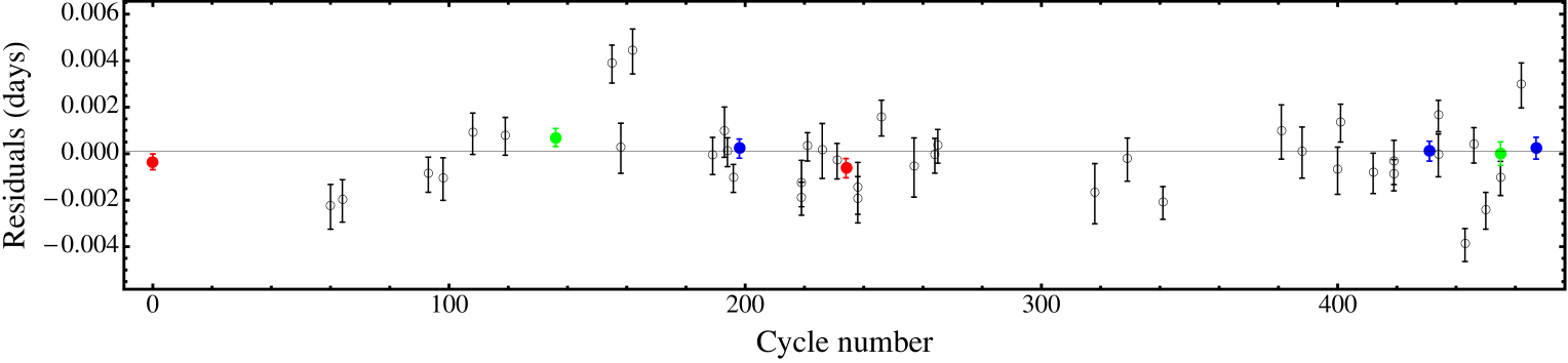
Figure 1: O$-$C diagramme for Qatar-1  transit times. The small symbols in colour refer to the Asiago (green), Calar Alto (blue) and Alsubai et al. (2011) (red) data used for redetermination of the ephemerides. Open circles represent transit times avaliable from the ETD.

4.2 Combined solution of photometric light-curves

The main parameters of the model are the fractional radii of the star and planet, r_⋆ and r_p, defined as the stellar radius $R_{\star}$ and the planetary radius $R_{\mathrm{p}}$ scaled by the semi-major axis $a$, respectively, and the orbital inclination $i_{p}$.

The LC solution was attempted using the linear and quadratic limb-darkening (LD) law, and with the LD coefficients either fixed at the theoretical values tabulated by Claret & Bloemen (2011) or included as fit parameters. We obtained the best result by fitting the LD($u_{1}$) coefficient using a linear law. We fitted individual light curves for the sum and ratio of the fractional radii $r_{\mathrm{p}}+r_{\star}$, $r_{\mathrm{p}}/r_{\star}$, the orbital inclination $i$, the central transit time $T_{0}$, and the limb darkening coefficient LD($u_{1}$). Evaluation of robust uncertainties on our best-fit parameters was performed by a bootstrap algorithm, i.e. generating for each light curve $10\,000$ resampled data sets to be fitted, and analysing the resulting distribution (Southworth et al. 2005). The light-curves and their best-fitting models are shown in Fig. 2, whereas the results of our analysis are reported in Table 4 along with the weighted means (WMs) for each parameter evaluated over all five transits. For some parameters ($r_{\mathrm{p}}/r_{\star}$ and LD($u_{1}$) the best-fit values are more scattered than expected by applying Gaussian statistics. A possible reason for these slight discrepancies could be intrinsic variations due to stellar activity of Qatar-1. Stellar spots, faculae and other active regions are known to alter the parameters inferred from photometric data, even when they are not occulted during the transit and thus no unusual feature is visible in the light curves (Ballerini et al. 2012). The ratio $r_{\mathrm{p}}/r_{\star}$ is one of the most critical parameters in this regard. We checked for long-term variability of Qatar-1 by performing differential photometry with the same comparison stars on the Asiago time series, A1 and A2, taken at the same site and airmass. We found a brightness variation between the two epochs of $+0.034\pm 0.005$ and $+0.030\pm 0.006$ mag (using two different reference stars), while the variation of our “check” star is $-0.004\pm 0.004$ mag. Although this finding is not fully conclusive, it suggests that stellar activity could play a role and possibly explain the differences in the LC solutions for different epochs.

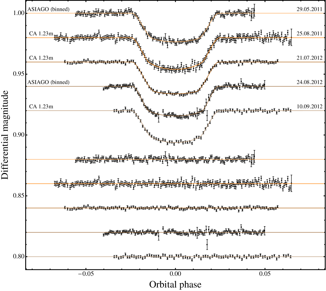
Figure 2: Photometric transit light-curves of Qatar-1 and corresponding residuals between data points and best-fit solution.

Table 4: Results from the analysis of individual and combined tranist light-curves

Date/ID	r⋆+rp	rp/ r⋆	$i_{\rm p}$	r⋆	rp	$b$	LD ($u_{1}$)
2011.05.29/A1	0.1850$\pm$0.0120	0.1441$\pm$0.0041	83.67$\pm$1.18	0.1617$\pm$0.0100	0.0233$\pm$0.0021	0.682$\pm$0.038	0.49$\pm$0.16
2012.08.24/A2	0.1716$\pm$0.0093	0.1431$\pm$0.0022	84.99$\pm$0.74	0.1501$\pm$0.0077	0.0215$\pm$0.0014	0.582$\pm$0.047	0.50$\pm$0.09
2011.08.25/C1	0.1793$\pm$0.0089	0.1465$\pm$0.0037	84.56$\pm$0.87	0.1564$\pm$0.0075	0.0229$\pm$0.0016	0.606$\pm$0.068	0.67$\pm$0.12
2012.07.21/C2	0.1882$\pm$0.0043	0.1535$\pm$0.0009	83.36$\pm$0.35	0.1632$\pm$0.0036	0.0250$\pm$0.0006	0.709$\pm$0.022	0.37$\pm$0.11
2012.09.10/C3	0.1834$\pm$0.0062	0.1496$\pm$0.0022	84.04$\pm$0.53	0.1595$\pm$0.0051	0.0239$\pm$0.0011	0.651$\pm$0.038	0.64$\pm$0.09
WM	0.1841$\pm$0.0030	0.1513$\pm$0.0008	83.82$\pm$0.25	0.1601$\pm$0.0025	0.0241$\pm$0.0005	0.675$\pm$0.016	0.54$\pm$0.05

N.B. : r_p = R_p/a; r_⋆ = R_⋆/a

4.3 Improved spectroscopic orbit solution

The 11 RV measurements corresponding to out-of-transit phases (see Table 1) form the data set we used to fit the spectroscopic orbit solution.

The solution of the RV curve was performed considering both the cases of circular and eccentric orbit. The results of our RV curve fits are summarised in Table 5, and the orbital solution corresponding to the fit obtained with the eccentricity as free parameter is shown in Fig. 3. The errors on the best-fit parameters were determined with the bootstrap method from 1000 mock data sets.

The comparison with the best-fit parameters reported in Alsubai et al. (2011) shows a number of significant differences. The Alsubai estimate of $\gamma$=-37835$\pm$63 m s^-1deviates from ours formally by more than 3$\sigma$. The most likely explanation for this discrepancy lies in a systematic RV zero-point difference between the two instruments used. The higher precision of the HARPS-N RV measurements allows us to rule out an eccentric orbit for Qatar-1 b. Our determination of $e=0.020^{+0.011}_{-0.010}$ is compatible with a circular orbit within 2$\sigma$, as expected for close-in planets with orbital periods shorter than a few days (Husnoo et al. 2012). Therefore, for the following analysis we adopted the best-fit parameters from the circular solution.

Finally, we obtained $K$=265.7 $\pm$ 3.5 m s^-1, which is about 20% higher than the value in Alsubai et al. (2011). Accordingly, the estimates of the mass and density of Qatar-1 b will be higher by the same percentage.

Table 5: Orbital parameters derived from the spectroscopic orbit solution of Qatar-1. The parameters that were kept fixed in the fit are in italics.

Orbital parameter
	Eccentric fit	Circular fit
$P$ [days]	1.42002504
$T_{0}$	—	2 456 174.46251
$T_{peri}$ [BJD]	$2\,456\,174.17^{+0.13}_{-0.19}$	—
$\gamma$ [m s-1]	$-$38051.7 $\pm$ 2.5	$-$38055.8 $\pm$ 2.0
$K_{\ast}$ [m s-1]	266.8 $\pm$ 3.4	265.7 $\pm$ 3.5
$e$	$0.020^{+0.011}_{-0.010}$	—
$a_{\ast}$ [km]	5220 $\pm$ 82
$\omega$ [deg]	$17^{+33}_{-47}$	—
$\chi^{2}$	1.184	1.380

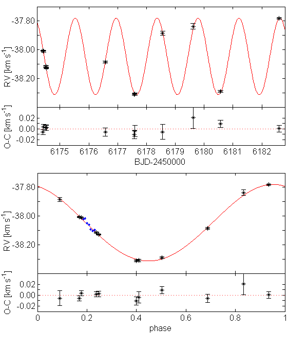
Figure 3: HARPS-N radial velocity data and best-fit spectroscopic orbit solution for Qatar-1. Upper panel: RV curve versus BJD showing only the out-of-transit data used for the orbital solution (solid red line), and the corresponding residuals. Lower panel: phase-folded RV curve (solid red line) and data used for the orbital fit drawn as black symbols. The RV measurements corresponding to in-transit phases are also displayed as light-blue symbols.

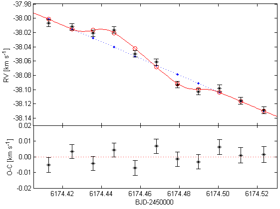
Figure 4: RM effect best-fit solution (solid, red line) with RV measurements (black star symbols) and computed RV values (red open circles), yielding the O$-$C beneath. The Keplerian radial velocity curve is also drawn as a blue dotted line.

4.4 Analysis of the RM effect and determination of the spin-orbit alignment

To analyse the RM effect we implemented a numerical model based on the following assumptions. We tried to reproduce the observed CCF by modelling the average photospheric line profile. The stellar disc is sampled by a matrix of 2000$\times$2000 elements, each element being represented by a Gaussian line profile with a given width $\sigma_{el}$, Doppler-shifted according to the stellar rotation, and weighted by appropriate limb-darkening coefficients. The resulting line profile is then convolved by the instrumental profile (assumed to be Gaussian) of HARPS-N, $\sigma_{IP}=1.108$ km s^-1. The model also takes into account the actual occulted area of the stellar photospheric disc and the smearing due to the planet’s displacement during an exposure. The corresponding RV shift is then computed by a Gaussian fit of this resulting line profile, analogously to the HARPS-N pipeline. The model depends on twelve parameters. The orbital period P_orb, mid-transit epoch $T_{0}$, transit duration $T_{14}$, star and planet radii R_⋆ and R_p, the linear limb-darkening coefficient LD$(u_{1})$, and the impact parameter $b$ were fixed to the values we derived from the light-curve solution, while the star RV semi-amplitude $K$ was set to the best-fit value obtained from the spectroscopic orbit with null eccentricity. The remaining parameters, i.e. the stellar projected rotational velocity v$\sin{I}$, the systemic velocity $\gamma$, the stellar disc resolution element line width $\sigma_{el}$, and the orbital obliquity $\lambda$ were treated as free parameters.

By using a “trust region” least-squares minimisation algorithm (Branch et al. 1999; Byrd et al. 1988), we obtained the following best-fit values: $\lambda=-8.4\pm 7.1$ deg, v$\sin{I}=1.7\pm 0.3$ km s^-1, $\sigma_{el}=2238\pm 155$ m s^-1, $\gamma=-38059.5\pm 2.0$ m s^-1, and normalised $\chi^{2}=1.217$. The errors were determined with the same bootstrap method as for the orbital RV curve fit from 200 mock data sets.

Although an independent determination of the systemic velocity $\gamma$ is provided by the orbital RV curve fit, we preferred to treat $\gamma$ as a free parameter, because of its strong correlation with the parameter $\lambda$ (see Fig. 5). In fact, by fixing the value of $\gamma$ to the value derived from the orbital RV curve fit, we obtained a best-fit value of $\lambda=-1^{\circ}$, with a normalised $\chi^{2}$ of 1.301. By letting $\gamma$ free to vary, we also allowed for a possible RV shift caused by stellar spots, whose configuration on the stellar disc can be assumed to remain constant over the time-span of the transit.

This analysis shows that the system is well aligned. The results are reported in Table LABEL:t:all_par. Fig. 5 shows the $\chi^{2}$-maps for various pairs of parameters.

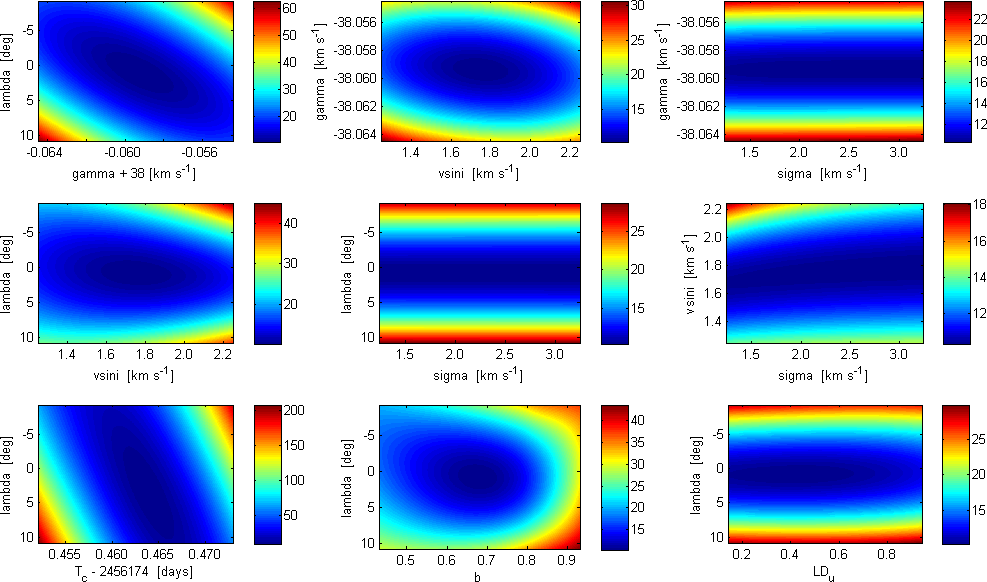
Figure 5: $\chi^{2}$-maps showing the correlation between different couples of parameters.

A preliminary calibration of the FWHM of the CCF in terms of projected rotational velocity based on a sample of stars with planets observed as part of GAPS yields v$\sin{I}$=1.6$\pm$0.5 km s^-1, consistent with the value derived as part of the RM effect modelling.

5 Characterisation of the host star

A proper determination of the stellar parameters is mandatory to obtain the physical properties of the planet.

Because of the uncertainty on the amount of interstellar extinction, photometric data alone cannot provide an accurate determination of the fundamental parameters of the star. According to the TASS Mark IV catalogue (Droege et al. 2006), the apparent V-band magnitude of Qatar-1 is V= 12.84 mag. The K2 V spectral type of the host star (from Alsubai et al. 2011) translates into an absolute magnitude of M_v=6.5 mag (Straizys & Kuriliene 1981). Depending on the amount of reddening, the distance to Qatar-1 is expected to span roughly between $\sim$190 pc for negligible extinction, and $\sim$130 pc for a normal interstellar extinction law (i.e., R${}_{\rm v}=3.1$) and the maximum colour excess value (i.e., E${}_{\rm B-V}=0.232\pm 0.003$) obtained from the reddening map by Schlegel et al. (1998).

5.1 Spectroscopic determination of stellar parameters

The HARPS-N spectra were used to perfom a spectroscopic characterisation of the host star Qatar-1 and estimate the effective temperature T_eff, surface gravity $\log{g}$, projected rotational velocity v$\sin{I}$, and the iron abundance [Fe/H]).

The effective temperature was initially determined from the HARPS-N spectra by applying the method of equivalent width (EW) ratios of spectral absorption lines by means of the ARES automatic code (Sousa et al. 2007), using the calibration for FGK dwarf stars by Sousa et al. (2010). For this purpose, we used an average spectrum of Qatar-1 obtained by a weighted mean of the 18 spectra available (after verifying that no contamination was present in the spectra taken with the simultaneous ThAr calibration), each properly shifted by the corresponding radial velocity to the rest wavelength frame, obtaining T${}_{\rm eff}=4990\pm 100$K.

Figure 6: Portion of Qatar-1 average spectrum (black solid line) and synthetic spectrum (red solid line) couplcorresponding to the following set of (fixed) parameters: $T_{\rm eff}=4910$ K, $\log g=4.66$, $\xi=0.90$ km s^-1, and $v\sin{I}=1.7$ km s^-1. The positions of five iron lines and two lines of titanium and calcium are marked. The inset shows a zoom on the spectral window containing three Fe i lines, and the comparison with synthetic spectra corresponding to [Fe i/H]=0.10 (green, long-dashed line), 0.20 (red, solid line), and 0.30 (blue, dotted line).

Furthermore, the atmospheric stellar parameters were derived using the program MOOG (Sneden 1973), version 2010, and through EW measurements of iron lines as described in detail by Biazzo et al. (2012). In particular, the effective temperature was determined by imposing the condition that the Fe i abundance does not depend on the excitation potential of the lines, the microturbulence velocity ($\xi$) was derived by imposing that the surface Fe i abundance is independent on the line EWs, and the surface gravity was estimated by imposing the Fe i/Fe ii ionization equilibrium. Then, we were also able to measure the iron abundance of Qatar-1. This analysis was performed differentially with respect to the Sun. For this purpose, we analysed the Qatar-1 spectrum and a Ganymede spectrum acquired with HARPS at ESO (Mayor et al. 2003). We thus obtained $\log n{({Fe\textsc{i}})_{\odot}}=\log n{({Fe\textsc{ii}})_{\odot}}=7.53\pm 0.05$ for the Sun. In the end, we found the following atmospheric parameters and iron abundance for the star: $T_{\rm eff}=4820\pm 100$ K, $\log g=4.43\pm 0.10$, $\xi=0.90\pm 0.05$ km s^-1, [Fe i/H]$=0.15\pm 0.10$, and [Fe ii/H]$=0.15\pm 0.08$, which agree with the previous determinations by Alsubai et al. (2011).

In addition, the stellar parameters were derived independently using the methodology presented in Santos et al. (2004) and Sousa et al. (2008). This analysis was also based on iron line excitation and ionization equilibrium, using a grid of Kurucz (1997) model atmospheres and the 2002 version of MOOG. The ARES code was used to measure the equivalent widths for a sub-set of iron lines from the list in Sousa et al. (2008) that is especially suited for determining the parameters of stars with temperature below 5200 K (for details see Tsantaki et al., A&A, submitted). The derived parameters are T_eff=4786$\pm$95 K, $\log{g}$=4.41$\pm$0.24, $\xi=0.78\pm 0.29$ km s^-1, and [Fe/H]=0.18$\pm$0.06. These values agree fairly well with those reported above.

As a final consistency check, we exploited the fact that there is only one temperature for which the surface gravity from evolutionary models will meet the one obtained from the ionization equilibrium. By imposing this condition, the surface gravity was obtained by comparison with the BaSTI evolutionary models. This yields the set of values $T_{\rm eff}=4910\pm 100$ K, $\log g=4.66\pm 0.10$, and [Fe /H]$=0.20\pm 0.10$. Fig. 6 shows the observed and the synthetic spectrum corresponding to the latter set of parameters and adopting for the projected rotational velocity the value $v\sin{I}=1.7$km $s^{-1}$, as derived from the RM best-fit solution (see Sect 4.4). This set of values was finally adopted by us in the following.

5.2 SED, reddening, and distance

We constructed the spectral energy distribution (SED) of Qatar-1 by merging the V and R optical magnitudes from the TASS Mark IV catalogue (Droege et al. 2006) with the infrared photometry from the 2MASS and WISE databases (Cutri et al. 2003; Cutri & et al. 2012), as shown in Fig. 7. We simultaneously fitted the colours encompassed by the SED to ad hoc synthetic magnitudes derived from a NextGen stellar atmosphere model (Hauschildt et al. 1999) with the same $T_{\rm eff}$, $log\,g$, and metallicity as the star. To estimate the interstellar extinction $A_{\rm v}$ and distance d to Qatar-1, we followed the method described in Gandolfi et al. (2008) and combined the availabe set of photometric data with the spectroscopically derived parameters. Assuming a total-to-selective extinction $R_{\rm v}=A_{\rm v}/E_{\rm B-V}=3.1$ and a black body emission at the star effective temperature and radius yields an extinction $A_{\rm v}=0.10\pm 0.10$ mag and a distance to the star $d=195\pm 25$ pc, fairly consistent with the range of values estimated above.

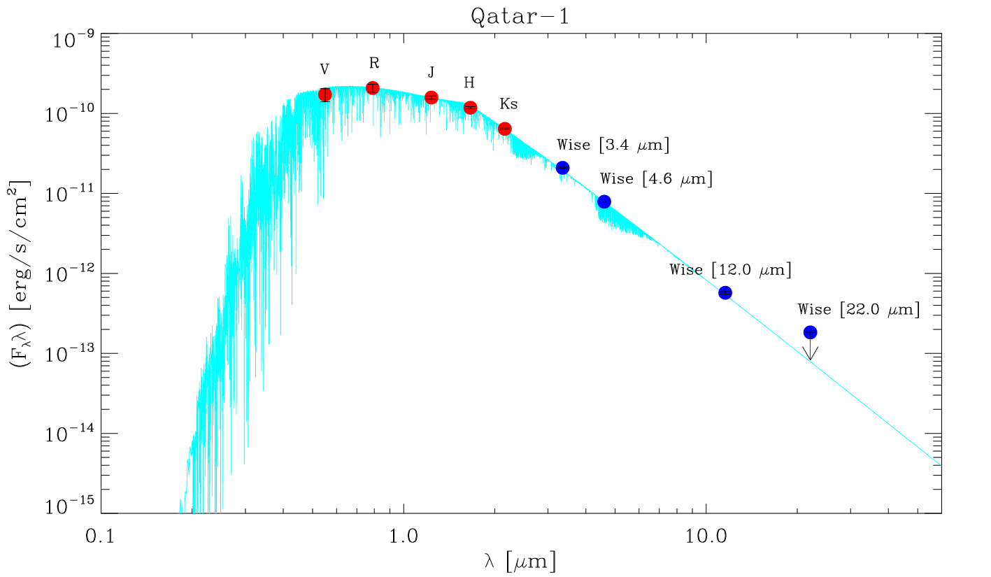
Figure 7: De-reddened spectral energy distribution of Qatar-1, for $A_{\rm v}=0.1$ and d=195 pc. Optical $V$ and $R$ photometric data are taken from the TASS Mark IV catalogue (Droege et al. 2006). Infrared data are taken from the 2MASS and WISE databases (Cutri et al. 2003; Cutri & et al. 2012). The NextGen synthetic low-resolution spectrum (Hauschildt et al. 1999) with the same photospheric parameters as Qatar-1 is over-plotted with a light-blue line.

Weak interstellar components are visible within the broad and blended Na i D_1,2 stellar doublet, as shown in Figure 8. Their equivalent widths are 0.017 and 0.009 ($\pm$0.001) Å, respectively, i.e. very close to the asymptotic 2.0 limit ratio for optically thin 5889.951 and 5895.924 Å lines. Some contamination from the adjacent not perfectly subtracted night-sky lines is possible. Adopting the Munari & Zwitter (1997) calibration between reddening and equivalent width of interstellar Na i 5889.951 Å line, the reddening affecting Qatar-1 is $E_{\rm B-V}$=0.004 ($\pm$0.0005).

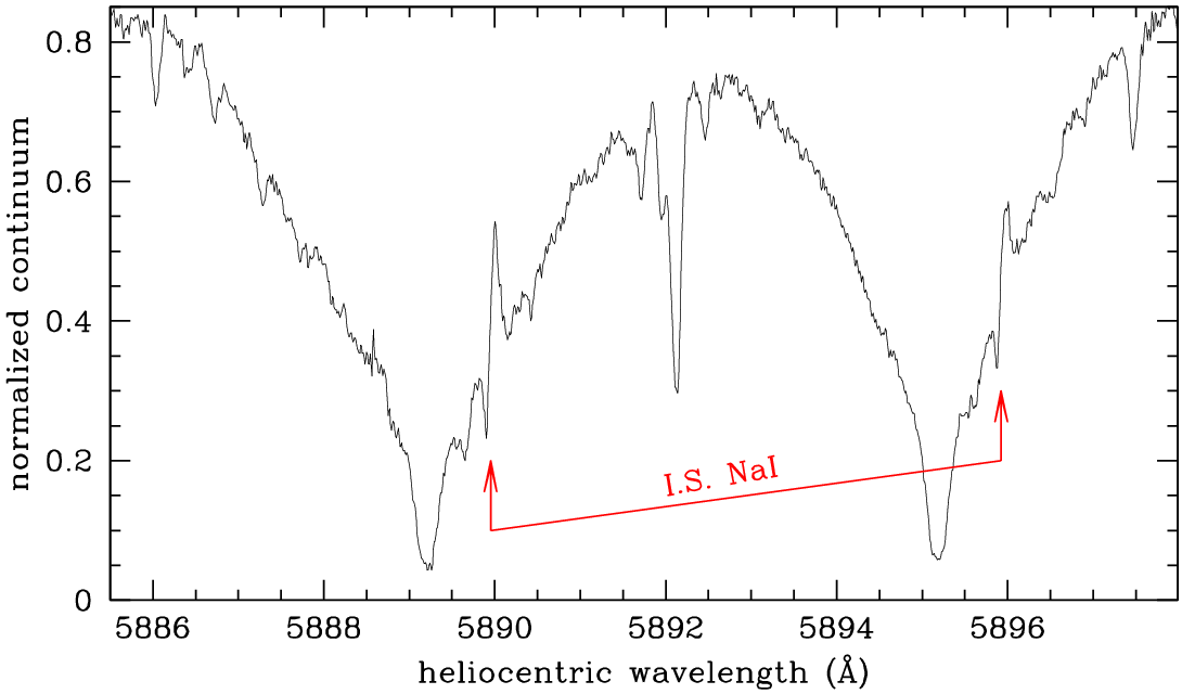
Figure 8: Portion of the HARPS-N averaged spectrum of Qatar-1 highlighting the weak interstellar Na i lines.

Finally, using a method based on the near-infrared SED published in Masana et al. (2006), as described in Section 2.3 of Ribas et al. (2010), and adopting the values of $\log{g}$ and [Fe/H] derived from the spectroscopic analysis (though their impact on the final values is very small, similarly to the immunity of the infrared flux method to those parameters), we obtained an effective temperature of T${}_{\mathrm{eff}}=4880\pm 70$ K. The main source of error is the uncertainty in the extinction value, assumed to be Av=0.1+/-0.1 mag. Hence, the resulting effective temperature perfectly agrees with the spectroscopic determination.

5.3 Star and planet physiscal properties

Table LABEL:t:all_par summarises the physical properties we derived for the star and the planet in the Qatar-1 system. To determine the stellar fundamental properties, we exploited quantities obtained directly from the analysis of the transit light curves following the prescriptions by Sozzetti et al. (2007). In particular, we derived the density of the star $\rho_{\star}=1.62\pm 0.08\rho_{\odot}$ from the scaled stellar radius $R_{\star}/a$ and used it together with T_eff and [Fe/H] obtained from the spectroscopic anaslysis to infer the stellar mass and radius by comparison with stellar evolution models. Using the BaSTI models, this yields a stellar mass $M_{\star}=0.85\,M_{\odot}\pm 0.03\,M_{\odot}$ and a radius $R_{\star}=0.80\pm 0.05\,R_{\odot}$, which coincide with the values reported by Alsubai et al. (2011). In turn, the surface gravity of the planet, $\log g_{\rm p}=3.372\pm 0.024$, and the planet equilibrium temperature, $T_{\rm P}=1389\pm 39$ K, with their corresponding uncertainties were obtained following Sozzetti et al. (2007) and Cowan & Agol (2011), respectively. The planetary radius and mass are found to be $1.18\pm 0.09$ R_J and $1.33\pm 0.05$ M_J. Hence, while only marginally larger in radius, the planet is found to be significantly more massive than reported by Alsubai et al. (2011).

6 Discussion

As discussed by Enoch et al. (2012), the radius of an exoplanet may be affected by a number of factors, which include the mass of the planet and its heavy element content as well as the irradiation received from the host star. For Qatar-1 b, we expect strong irradiation and tidal effects because of its proximity to the host star. Below, we examine rotation and activity indicators and discuss the possible evolutionary effects caused by tidal interaction.

Table 6: Summary of planet and star parameters for the Qatar-1 system.

Parameter [Units]	Symbol	Value	Method
Transit epoch (BJD_TCB$-$2450000.0) [days]	$T_{0}$	$5518.41094\pm 0.00016$	(1)
Orbital period [days]	$P$	$1.42002504\pm 0.00000071$	(1)
Transit duration [days]	$T_{14}$	$0.0678\pm 0.0010$	(2)
Planet/star area ratio	$(R_{\rm p}/R_{\star})^{2}$	$0.02280\pm 0.00011$	(2)
Planet/star radii ratio	$R_{\rm p}/R_{\star}$	$0.1513\pm 0.0008$	(2)
Orbital inclination [degrees]	$i_{\rm p}$	$83.82\pm 0.25$	(2)
Impact parameter	$b$	$0.675\pm 0.016$	(2)
Scaled stellar radius	$R_{\star}/a$	$0.1601\pm 0.0025$	(2)
Scaled planet radius	$R_{p}/a$	$0.0241\pm 0.0005$	(2)
Star reflex velocity [km s-1]	$K_{\star}$	$0.2657\pm 0.0035$	(3)
Orbital eccentricity	$e$	$0$	(3)
Systemic velocity [km s-1]	$\gamma$	$-38.0558\pm 0.0002$	(3)
Star density [$\rho_{\odot}$]	$\rho_{\star}$	$1.62\pm 0.08$	(4)
Planet surface gravity [cgs]	$\log g_{\rm p}$	$3.372\pm 0.024$	(4)
Star mass [M⊙]	$M_{\star}$	$0.85\pm 0.03$	(5)
Planet mass [MJ]	$M_{\rm p}$	$1.33\pm 0.05$	(6)
Orbital semi-major axis [AU]	$a$	$0.02343\pm 0.0012$	(7)
Star radius [R⊙]	$R_{\star}$	$0.80\pm 0.05$	(7)
Star surface gravity	$\log g_{\star}$	$4.55\pm 0.10$	(7)
Planet radius [RJ]	$R_{\rm p}$	$1.18\pm 0.09$	(7)
Planet density [$\rho_{\rm J}$]	$\rho_{\rm p}$	$0.80\pm 0.20$	(7)
Spin-orbit misalignment [degrees]	$\lambda$	$-8.4\pm 7.1$	(8)
Star projected rotational velocity [km s-1]	v$\sin{I}$	$1.7\pm 0.3$	(8)
Star effective temperature [K]	$T_{\rm eff}$	$4910\pm 100$	(9)
Stellar metallicity	[Fe/H]	$0.20\pm 0.10$	(9)
Star age [Gyr]	$Age_{\star}$	$\approx 4.5$	(10)
Planet equilibrium temperature [K]	$T_{\rm P}$	$1389\pm 39$	(11)

(1) Derived by combining the determinations of the mid-transit times from our photometric data sets with those derived from Alsubai et al. (2011). Kept fixed in the orbital and Rossiter RV fitting. (2) Derived as weighted mean of the best-fit determinations from our five transit light curves. (3) Derived by fitting the orbital RV curve to out-of-transit RV measurements. (4) Derived following Sozzetti et al. (2007). (5) Derived from evolutionary models. (6) Derived by using the expression of the mass function. (7) Derived from parameters above. (8) Derived by fitting our RM effect model to in-transit RV measurements. (9) Derived from spectroscopic analysis. (10) Derived from gyrochronology. (11) Derived following Cowan & Agol (2011).

6.1 Stellar rotation, activity, and age

Adopting the v$\sin{I}$ of $1.7\pm 0.3$ km s^-1 and radius of $0.80\pm 0.05$ R_⊙ for Qatar-1, and assuming that the star is viewed equator-on, the rotation period is calculated to be $24\pm 6$  days. The gyrochronological age, $t_{gyro}$, can hence be estimated using the relation given by Barnes (2007) (equation 3). For a ${\rm(B-V)}=0.9$, corresponding to a $T_{\rm eff}$ of 4910 K of the star, we obtain $t_{gyro}=1.7\pm 1.1$ Gyr.

On the other hand, adopting the revised gyrochronology by Lanza (2010) for stars with hot Jupiters, we estimate an age of $\sim 4.5$ Gyr that better agrees with that derived from stellar evolutionary tracks (cf. Fig. 5 of Alsubai et al. 2011).

Chromospheric emission is present in the Ca ii H&K lines. Unfortunately, the S/N of individual HARPS-N spectra in the wavelength range below 4000Å is inadequate to obtain reliable measurements of the $\log R^{\prime}_{HK}$ index. Therefore it is not possible to look for eventual variations in the chromospheric activity. However, using the passband definitions in Duncan et al. (1991) and a preliminary calibration of the flux in the Ca ii H&K lines, we obtained S${}_{HK}=0.389$ from the average spectrum used in Sec. 5.1. Then, by adopting ${\rm(B-V)}=0.9$ and the calibrations of Noyes et al. (1984), we find $\log{\rm R^{\prime}_{HK}}=-4.60$. Therefore, Qatar-1 appears to be a moderately active star, similar to, e.g., HD 189733 and TrES-3 (Knutson et al. 2010).

Using the relations given by Noyes et al. (1984) and Mamajek & Hillenbrand (2008), the expected rotation period for $\log{\rm R^{\prime}_{HK}}=-4.60$ and ${\rm(B-V)}=0.9$ would be 23.8 d and 23.0 d, respectively, hence within the range estimated from v$\sin{I}$. However, using relation (3) from Mamajek & Hillenbrand (2008) of age as a function of $\log{\rm R^{\prime}_{HK}}$, yields an age of about 1.1 Gyr, which is considerably younger than the value inferred from gyrochronology (see also Pace 2013 for an updated analysis on the use of chromospheric activity as an age indicator).

Finally, we note that Qatar-1 b fits well within the $\log{\rm R^{\prime}_{HK}}$-$\log g_{\rm p}$ correlation pointed out by Hartman (2010) for close-in planets ($a<0.1$ AU) with $M_{\rm p}>0.1$ $M_{\rm J}$, orbiting stars with 4200 K$<T_{\rm eff}<6200$ K. It appears also to be consistent with the indication reported by Krejčová & Budaj (2012) that the level of the chromospheric activity of stars with $T_{\rm eff}<5500$ K hosting close-in planets ($a<0.15$ AU) may be enhanced by the presence of Jupiter-mass planets.

6.2 Star–planet tidal interaction

The orbital period of the planet in the Qatar-1 system is much shorter than the rotation period of the star estimated in Sec. 6.1. Therefore, tides produce a decay of the orbit with a continuous transfer of angular momentum from the orbital motion to the spin of the star. The orbital angular momentum is only 0.28 of the present stellar spin, which is insufficient to reach an equilibrium synchronous state. In other words, as a consequence of the tidal evolution, the planet is expected to be engulfed by the star. The timescale for the orbital decay $\tau_{\rm a}^{-1}\equiv(1/a)(da/dt)$, where $a$ is the orbital semi-major axis and $t$ the time, depends on the efficiency of the tidal dissipation inside the star that is parameterised by its modified tidal quality factor $Q^{\prime}_{\rm s}$. Considering the tidal dissipation efficiency required to account for orbital circularisation and synchronisation in close binary systems, Ogilvie & Lin (2007) estimated that $Q^{\prime}_{\rm s}$ is of the order of $10^{6}$ for late-type main-sequence stars. Adopting this value and the stellar and planetary parameters in Table LABEL:t:all_par, we obtain $\tau_{\rm a}\sim 0.5$ Gyr for Qatar-1 using the tidal evolutionary model of Leconte et al. (2010). The timescale for the alignment of the orbital angular momentum and the stellar spin can be estimated from the same tidal model and is $\tau_{\epsilon}^{-1}\equiv(1/\epsilon)(d\epsilon/dt)$, where $\epsilon$ is the obliquity of the stellar equator with respect to the orbital plane. Assuming $Q^{\prime}_{\rm s}=10^{6}$ and an initial obliquity $\epsilon(t=0)=30^{\circ}$ yields $\tau_{\epsilon}\approx 0.2$ Gyr.

It is interesting to note that the timescale of orbital decay computed with $Q^{\prime}_{\rm s}=10^{6}$ is significantly shorter than the estimated age of the star from Sect 6.1. The difference is not as dramatic as in the case of, e.g., OGLE-TR-56 (Ogilvie & Lin 2007), or Kepler-17 (Bonomo & Lanza 2012), where the orbital decay timescale turns out to be as short as 40-70 Myr, but this result suggests that the use of the same value of $Q^{\prime}_{\rm s}$ as derived for close stellar binary systems also for star-planet systems is not appropriate (cf. other analyses trying to constrain $Q_{\rm s}^{\prime}$, e.g., Pätzold & Rauer 2002; Ogilvie & Lin 2007; Carone & Pätzold 2007; Jackson et al. 2009; Pätzold et al. 2012). In principle, a lower limit on $Q^{\prime}$ can be established by an accurate timing of the transits extended over a baseline of several decades, which allows one to test the predictions of the above models. Specifically, for $Q^{\prime}_{\rm s}=10^{6}$, the orbital decay is expected to produce a variation of the observed epoch of mid-transit with respect to a constant-period ephemeris of $O-C\sim 17$ s in twenty years.

The tidal evolution of stellar obliquity has been recently discussed by Lai (2012) from a theoretical point of view, and by Albrecht et al. (2012) considering RM observation statistics.

7 Summary and conclusions

We reported on observations of the RM effect for the Qatar-1 system and a new determination of the orbital solution based on HARPS-N at TNG observations. With these data we also obtained the spectroscopic characterisation of the host star. Combining the radial velocity data with new transit photometry and with photometric data from the literature, we derived new ephemerides and improved the orbital parameters for the system. The most notable results from this analysis can be summarised as follows:

1. The new spectroscopic orbital solution is found to be consistent with a circular orbit and any significant eccentricity of the orbit can be ruled out.

2. The RM effect was measured and the sky-projected obliquity was determined, from which we can conclude that the orbital plane of the system is well-aligned with the spin axis of the star. This result and the derived properties of Qatar-1 b appear to be in line with the general trend observed for close-in planets around stars cooler than about 6250 K (Albrecht et al. 2012).

3. The host star is confirmed to be a slowly rotating, metal-rich K-dwarf, which yet is found to be moderately active, as inferred from the strength of the chromospheric emission in the Ca II H&K line cores and from changes in the photometric light-curves at different epochs, which hint at the presence of stellar spots.

4. The planet is found to be significantly more massive than previously estimated by Alsubai et al. (2011).

5. Qatar-1 appears to be consistent with the indication that the level of the chromospheric activity in stars cooler than 5500 K that host close-in giant planets may be enhanced. An attempt at estimating the timescale for the orbital decay by tidal dissipation was also presented, which deserves further investigation.