Tropical convexity over max-min semiring

Abstract.

This is a survey on an analogue of tropical convexity developed over the max-min semiring, starting with the descriptions of max-min segments, semispaces, hyperplanes and an account of separation and non-separation results based on semispaces. There are some new results. In particular, we give new “colorful” extensions of the max-min Carathéodory theorem. In the end of the paper, we list some consequences of the topological Radon and Tverberg theorems (like Helly and Centerpoint theorems), valid over a more general class of max-T semirings, where multiplication is a triangular norm.

1. Introduction

The max-min semiring is defined as the unit interval ${\mathcal{B}}=[0,1]$ with the operations $a\oplus b:=\max(a,b)$, as addition, and $a\otimes b:=\min(a,b)$, as multiplication. The operations are idempotent, $\max(a,a)=a=\min(a,a)$, and related to the order:

(1.1) $$\max(a,b)=b\Leftrightarrow a\leq b\Leftrightarrow\min(a,b)=a.$$

One can naturally extend them to matrices and vectors leading to the max-min (fuzzy) linear algebra [3, 6, 7]. We denote by ${\mathcal{B}}(d,m)$ the set of $d\times m$ matrices with entries in ${\mathcal{B}}$ and by ${\mathcal{B}}^{d}$ the set of $d$-dimensional vectors with entries in ${\mathcal{B}}$. Both ${\mathcal{B}}(d,m)$ and ${\mathcal{B}}^{d}$ have a natural structure of semimodule over the semiring ${\mathcal{B}}$.

The max-min segment between $x,y\in{\mathcal{B}}^{d}$ is defined as

(1.2) $$\ [x,y]_{\oplus} =\{\alpha\otimes x\oplus\beta\otimes y\mid\,\alpha\oplus\beta=1,\alpha,\beta\in{\mathcal{B}}\}.\$$

A set $C\subseteq{\mathcal{B}}^{d}$ is called max-min convex, if it contains, with any two points $x,y,$ the segment $[x,y]_{\oplus}$ between them. For a general subset $X\subseteq{\mathcal{B}}^{d}$, define its convex hull $\operatorname{conv}_{\oplus}(X)$ as the smallest max-min convex set containing $X$, i.e., the smallest set containing $X$ and stable under taking segments (1.2). As in the ordinary convexity, $\operatorname{conv}_{\oplus}(X)$ is the set of all max-min convex combinations

(1.3) $$\bigoplus_{i=1}^{m}\lambda_{i}\otimes x^{i}\colon m\geq 1,\ \bigoplus_{i=1}^{m}\lambda_{i}=1,$$

of all $m$-tuples of elements $x^{1},\ldots,x^{m}\in X$. The max-min convex hull of a finite set of points is also called a max-min convex polytope.

A (max-min) semispace at $x\in{\mathcal{B}}^{d}$ is defined as a maximal max-min convex set not containing $x$. A straightforward application of Zorn’s Lemma shows that if $C\subseteq{\mathcal{B}}^{d}$ is convex and $x\notin C$, then $x$ can be separated from $C$ by a semispace. It follows that the semispaces constitute the smallest intersectional basis of max-min convex sets. This fact is true more generally in abstract convexity. Some new phenomena appear in max-min convexity, which further emphasize the importance of semispaces in any convexity theory. For example, separation of a point and a convex set by hyperplanes is not always possible in max-min convexity [12], [13].

The max-min segments and semispaces were described, respectively, in [16, 19] and in [17]. In the present paper, the max-min segments are introduced in Section 2. We recall the structure of max-min semispaces in Section 3 together with some immediate consequences from abstract convexity. In [13, 14] further progress is made in the study of max-min convexity focusing on the role of semispaces. Being motivated by the Hahn-Banach separation theorems in the tropical (max-plus) convexity [21] and extensions to functional and abstract idempotent semimodules [4, 11, 22], we compared semispaces to max-min hyperplanes in [13], and developed an interval extension of separation by semispaces in [14]. These results are summarized in Section 4. Another principal goal of this paper is to investigate classical convexity results such as the theorems of Carathéodory, Helly and Radon in the realm of max-min convexity. These results are presented in Sections 5, 6 and 7 and are inspired by a paper of Gaubert and Meunier [8], in which similar statements can be found for the case of max-plus convexity. The max-min Carathéodory theorem with some “colorful” extensions is presented in Section 5. The strongest extension relies on what we call the internal separation theorem, which is proved in Section 6. In the last section, motivated by the fuzzy algebra of [10], we consider a more general class of max-T semirings, where the role of multiplication is played by a triangular norm. We show how the topological Radon and Tverberg theorems can be applied to obtain, in particular, the max-min analogues of Radon, Helly, Centerpoint and (in part) Tverberg theorems.

2. Description of segments

In this section we describe general segments in ${\mathcal{B}}^{d},$ following [16, 19], where complete proofs can be found. Note that the description of the segments in [16, 19] is done for the equivalent case where ${\mathcal{B}}=[-\infty,+\infty]$.

Let $x=(x_{1},...,x_{d}),$ $y=(y_{1},...,y_{d})\in{\mathcal{B}}^{d},$ and assume that we are in the case of comparable endpoints, say $x\leq y$ in the natural order of ${\mathcal{B}}^{d}.$ Sorting the set of all coordinates $\{x_{i},y_{i},i=1,...,d\}$ we obtain a non-decreasing sequence, denoted by $t_{1},t_{2},\ldots,t_{2d}$. This sequence divides the set ${\mathcal{B}}$ into $2d+1$ subintervals $\sigma_{0}=[0,t_{1}],\,\sigma_{1}=[t_{1},t_{2}],...,\sigma_{2d}=[t_{2d},1]$, with consecutive subintervals having one common endpoint.

Every point $z\in[x,y]_{\oplus}$ is represented as $z=\alpha\otimes x\oplus\beta\otimes y$, where $\alpha=1$ or $\beta=1$. However, case $\beta=1$ yields only $z=y$, so we can assume $\alpha=1$. Thus $z$ can be regarded as a function of one parameter $\beta$, that is, $z(\beta)=(z_{1}(\beta),...,z_{d}(\beta))$ with $\beta\in{\mathcal{B}}$. Observe that for $\beta\in\sigma_{0}$ we have $z(\beta)=x$ and for $\beta\in\sigma_{2d}$ we have $z(\beta)=y$. Vectors $z(\beta)$ with $\beta$ in any other subinterval form a conventional elementary segment. Let us proceed with a formal account of all this.

Theorem 1.

Let $x,y\in{\mathcal{B}}^{d}$ and $x\leq y$.

• We have

  (2.1) $$[x,y]_{\oplus}=\bigcup_{l=1}^{2d-1}\{z(\beta)\mid\beta\in\sigma_{l}\},$$

  where $z(\beta)=x\oplus(\beta\otimes y)$ and $\sigma_{\ell}=[t_{l},t_{l+1}]$ for $\ell=1,\ldots,2d-1$, and $t_{1},\ldots,t_{2d}$ is the nondecreasing sequence whose elements are the coordinates $x_{i},y_{i}$ for $i=1,\ldots,d$.

• For each $\beta\in{\mathcal{B}}$ and $i$, let $M(\beta)=\{i\colon x_{i}\leq\beta\leq y_{i}\}$, $H(\beta)=\{i\mid\beta\geq y_{i}\}$ and $L(\beta)=\{i\colon\beta\leq x_{i}\}$. Then

  (2.2) $$z_{i}(\beta)=\begin{cases}\beta,&\text{if $i\in M(\beta)$},\\ x_{i},&\text{if $i\in L(\beta)$},\\ y_{i},&\text{if $i\in H(\beta)$},\end{cases}$$

  and $M(\beta),L(\beta),H(\beta)$ do not change in the interior of each interval $\sigma_{\ell}$.

• The sets $\{z(\beta)\mid\beta\in\sigma_{\ell}\}$ in (2.1) are conventional closed segments in ${\mathcal{B}}^{d}$ (possibly reduced to a point), described by (2.2) where $\beta\in\sigma_{\ell}$.

For incomparable endpoints $x\not\leq y,\,y\not\leq x,$ the description can be reduced to that of segments with comparable endpoints, by means of the following observation.

Theorem 2.

Let $x,y\in{\mathcal{B}}^{d}$. Then $[x,y]_{\oplus}$ is the concatenation of two segments with comparable endpoints, namely $[x,y]_{\oplus}=[x,x\oplus y]_{\oplus}\cup[x\oplus y,y]_{\oplus}.$

All types of segments for $d=2$ are shown in the right side of Figure 1.

The left side of Figure 1 shows a diagram, where for $x=(x_{1},x_{2},x_{3})$ and $y=(y_{1},y_{2},y_{3})$, the segments $[x_{1},y_{1}],[x_{2},y_{2}],$ and $[x_{3},y_{3}]$ are placed over one another, and their arrangement induces a tiling of the horizontal axis, which shows the possible values of the parameter $\beta$. The partition of the real line induced by this tiling is associated with the intervals $\sigma_{l}$, and the sets of active indices $i$ with $z_{i}(\beta)=\beta$ associated with each $\sigma_{l}$ are also shown.

Figure 1. Max-min segments.

Remark 1.

We observe that, similarly to the max-plus case (see [15], Remark 4.3) in ${\mathcal{B}}^{d}$ there are elementary segments in only $2^{d}-1$ directions. Elementary segments are the ”building blocks” for the max-min segments in ${\mathcal{B}}^{d},$ in the sense that every segment $[x,y]\subset{\mathcal{B}}^{d}$ is the concatenation of a finite number of elementary subsegments (at most) $2d-1$, respectively $2d-2$, in the case of comparable, respectively incomparable, endpoints.

Max-min segments allow to introduce a natural metric on ${\mathcal{B}}^{d}$ ([9]). More precisely, one defines the distance between two points to be the Euclidean length of the max-min segment joining them.

3. Description of semispaces

For any point $x^{0}=(x_{1}^{0},\dots,x_{d}^{0})\in{\mathcal{B}}^{d}$ we define a finite family of subsets $S_{0}(x^{0}),\dots,S_{d}(x^{0})$ in ${\mathcal{B}}^{d}$. These subsets were shown to be semispaces in [17, Proposition 4.1]. A point $x^{0}$ is called finite if it has all coordinates different from zeros and ones. This definition is motivated by the isomorphic version of max-min algebra where the least element (and zero of the semiring) is $-\infty$, and the greatest element (and unity of the semiring) is $+\infty$.

Without loss of generality we may assume that $x^{0}$ is non-increasing: $x_{1}^{0}\geq\dots\geq x_{d}^{0}.$ Writing this more precisely we have

(3.1) $$\begin{gathered}x_{1}^{0}=\dots=x_{k_{1}}^{0}>\dots>x_{k_{1}+l_{1}+1}^{0}=\dots=x_{k_{1}+l_{1}+k_{2}}^{0}>\dots{\\ }>x_{k_{1}+l_{1}+k_{2}+l_{2}+1}^{0}=\dots=x_{k_{1}+l_{1}+k_{2}+l_{2}+k_{3}}^{0}>\dots{\\ }>x_{k_{1}+l_{1}+\dots+k_{p-1}+l_{p-1}+1}^{0}=\dots=x_{k_{1}+l_{1}+\dots+k_{p-1}+l_{p-1}+k_{p}}^{0}\\ >\dots>x^{0}_{k_{1}+l_{1}+\dots+k_{p}+l_{p}}(=x^{0}_{d}),\end{gathered}$$

where $\sum_{j=1}^{p}(k_{j}+l_{j})=d$, $k_{1}=0$ if the sequence (3.1) starts with strict inequalities and $l_{p}=0$ if the sequence ends with equalities.

Let us introduce the following notations:

$$\begin{split}L_{0}&=0,K_{1}=k_{1},L_{1}=K_{1}+l_{1}=k_{1}+l_{1},\\ K_{j}&=L_{j-1}+k_{j}=k_{1}+l_{1}+...+k_{j-1}+l_{j-1}+k_{j}\quad(j=2,...,p),\\ L_{j}&=K_{j}+l_{j}=k_{1}+l_{1}+...+k_{j}+l_{j}\quad(j=2,...,p);\end{split}$$

we observe that $l_{j}=0$ if and only if $K_{j}=L_{j}.$

We are ready to define the subsets. We need to distinguish the cases when the sequence (3.1) ends with zeros or begin with ones, since some subsets $S_{i}$ become empty in that case.

Definition 1.

Let $x^{0}\in{\mathcal{B}}^{d}$ be a non-increasing vector
a) If $x^{0}$ has $0<x_{i}^{0}<1$ for all $1\leq i\leq d$, then define:

$$\begin{split}S_{0}(x^{0})=&\{x\in{\mathcal{B}}^{d}|x_{i}>x_{i}^{0}\text{ for some }1\leq i\leq d\},\\ S_{K_{j}+q}(x^{0})=&\{x\in{\mathcal{B}}^{d}|x_{K_{j}+q}<x_{K_{j}+q}^{0},\text{ or }x_{i}>x_{i}^{0}\\ &\text{ for some }K_{j}+q+1\leq i\leq d\}(q=1,...,l_{j};j=1,...,p\text{ if }l_{j}\neq 0),\\ S_{L_{j-1}+q}(x^{0})=&\{x\in{\mathcal{B}}^{d}|x_{L_{j-1}+q}<x_{L_{j-1}+q}^{0},\text{ or }x_{i}>x_{i}^{0}\\ &\text{ for some }K_{j}+1\leq i\leq d\}\\ &(q=1,...,k_{j};j=1,...,p\text{ if }k_{1}\neq 0,\text{ or }j=2,...,p\text{ if }k_{1}=0).\end{split}$$

b) If there exists an index $i\in\{1,...,d\}$ such that $x_{i}^{0}=1,$ but no index $j$ such that $x_{j}^{0}=0,$ then define the subsets $S_{1},...,S_{d}$ as in part a).

c) If there exists an index $j\in\{1,...,d\}$ such that $x_{j}^{0}=0,$ but no index $i$ such that $x_{i}^{0}=1,$ then define the subsets $S_{0},S_{1},...,S_{\beta-1}$ as in part a), where $\beta:=\min\{1\leq j\leq n|\;x_{j}^{0}=0\}.$

d) If there exists an index $i\in\{1,...,d\}$ such that $x_{i}^{0}=1,$ and an index $j$ such that $x_{j}^{0}=0,$ then define the subsets $S_{1},...,S_{\beta-1}$ as in part a), where $\beta:=\min\{1\leq j\leq n|\;x_{j}^{0}=0\}.$

Let now $x^{0}\in{\mathcal{B}}^{d}$ have arbitrary order of coordinates, and let us formally extend Definition 1. For this, consider a permutation $\pi$ of the index set $\{1,\ldots,d\}$ such that the vector $(x_{\pi(1)},x_{\pi(2)},\ldots,x_{\pi(d)})$ is non-increasing. Let $\overline{\pi}:{\mathcal{B}}^{d}\to{\mathcal{B}}^{d}$ be the invertible map of ${\mathcal{B}}^{d}$ induced by the permutation $\pi$. Then we can define $S_{i}(x^{0})=\overline{\pi}^{-1}(S_{j}(\overline{\pi}(x^{0})))$, where $j=\pi(i)$.

Further, for any $x^{0}\in{\mathcal{B}}^{d}$ we denote by $I(x^{0})$ the set of indices $i$ such that $S_{\pi(i)}(\overline{\pi}(x^{0}))$ is present in Definition 1. Observe that $I(x^{0})$ consists of the indices $i$ such that $x^{0}_{i}>0$ and, possibly, $0$.

Pictures of all semispaces at a finite point for $d=2$ are shown in Figure 2.

Figure 2. Semispaces in ${\mathcal{B}}^{2}$ at a finite point

The following theorem is the main result in [17]. See also [14].

Theorem 3.

For any $p\in{\mathcal{B}}^{d}$ the sets $S_{i}(p),i\in I(p),$ are maximal (with respect to the set inclusion) max-min convex avoiding the point $p$. Thus for any $p\in{\mathcal{B}}^{d}$, there exists at least one and at most $d+1$ semispaces $S_{i}(p),0\leq i\leq d,$ at $p$.

For all $C\subseteq{\mathcal{B}}^{d}$ max-min convex and any $p\in{\mathcal{B}}^{d}\setminus C$, there exists a semispace $S_{i}(p)$ such that $C\subseteq S_{i}(p)$ and $p\not\in S_{i}(p)$.

The complement of a semispace $S_{i}(p)$ is denoted by $\complement S_{i}(p)$. These complements are also called sectors, in analogy with the max-plus convexity.

The lemma below follows from the abstract definition of the semispaces and it is our main tool in extending Carathéodory theorem and its colorful versions to the max-min setup. As only a finite number of semispaces at a given point exist, the max-min convexity can be regarded as a multiorder convexity [16, 17].

Lemma 1 (Multiorder principle).

Let $X\subseteq{\mathcal{B}}^{d}$ and $p\in{\mathcal{B}}^{d}$. Then the following statements are equivalent:

1. $p\in\operatorname{conv}_{\oplus}(X)$;

2. for all $i\in I(p),$ there exists $x^{i}\in X$ such that $x^{i}\in\complement S_{i}(p)$.

Proof.

(i) $\rightarrow$ (ii) By contradiction. Assume there is $i_{0}\in I(p)$ such that $X\cap\complement S_{i_{0}}(p)=\emptyset$. Then $p\in\operatorname{conv}_{\oplus}(X)\subseteq S_{i_{0}}(p)$, in contradiction to $p\not\in S_{i_{0}}(p)$.

(ii) $\rightarrow$ (i) By contradiction. Assume that $p\not\in\operatorname{conv}_{\oplus}(X)$. As $\operatorname{conv}_{\oplus}(X)$ is a convex set, it follows from Theorem 3 that there exists $i_{0}\in I(p)$ such that $\operatorname{conv}_{\oplus}(X)\subseteq S_{i_{0}}(p)$, which implies $\complement S_{i_{0}}(p)\subseteq\complement\operatorname{conv}_{\oplus}(X)$. But from (ii), there exists $x_{i^{0}}\in\complement S_{i_{0}}(p)\cap\operatorname{conv}_{\oplus}(X)$, which gives a contradiction. ∎

4. Separation and non-separation

In what follows ${\mathcal{B}}^{d}$ has the usual Euclidean topology. If $A\subseteq{\mathcal{B}}^{d}$, we denote by $\overline{A}$ the closure of $A$, by $\text{int}(A)$ the interior of $A$ and by $\complement A$ the complement of $A$.

In the tropical convexity, all semispaces are open tropical halfspaces expressed as solution sets to a strict two-sided max-linear inequality. See e.g. [15]. Thus the closures of semispaces are hyperplanes.

In the case of max-min convexity, hyperplane in ${\mathcal{B}}^{d}$ can be defined as the solution set to a max-min linear equation

(4.1) $$\max(\min(a_{1},x_{1}),\ldots,\min(a_{d},x_{d}),a_{d+1})=\max(\min(b_{1},x_{1}),\ldots,\min(b_{d},x_{d}),b_{d+1}).$$

The structure of a max-min hyperplane is presented in [12]. One investigates the distribution of values for the left and right hand side of (4.1), and then identifies the regions in ${\mathcal{B}}^{d}$ where the values of the sides coincide. We illustrate this procedure in Figure 3, which shows the structure of a max-min hyperplane (line) in ${\mathcal{B}}^{2}$. The left side pictures show the distribution of values for both sides of (4.1): for the white regions the distribution is uniform and the value is equal to the coordinate of the finite point on the main diagonal that belongs to their boundary; the regions labeled $x_{1}$ are tiled by vertical lines for which the value of each point is equal to its $x_{1}$ coordinate, and the regions labeled $x_{2}$ are tiled by horizontal lines for which the value of each point is equal to its $x_{2}$ coordinate. The right side picture shows the graph of the line.

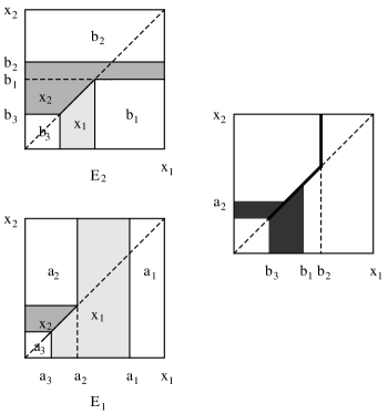
Figure 3. A max-min hyperplane (line) in ${\mathcal{B}}^{2}$.

In [13] we investigated the relation between the max-min hyperplanes and the closures of semispaces ${S}_{i}(x)$. We recall that the diagonal of ${\mathcal{B}}^{d}$ is the set ${\mathcal{D}}_{d}=\{(a,\ldots,a)\in{\mathcal{B}}^{d}\mid a\in{\mathcal{B}}\}.$

Theorem 4 ([13], Theorem 3.1).

A closure of semispace is a hyperplane if and only if it can be represented as $\overline{S}_{i}(y)$ for some $y$ belonging to the diagonal.

Recall that a set $C\subset{\mathcal{B}}^{d}$ is separated from a point $x\in{\mathcal{B}}^{d}$ by a hyperplane $H\subset{\mathcal{B}}^{d}$ if $C\subset H$ and $x\not\in H$. Theorem 4 shows exactly when classical separation by hyperplanes is possible.

Corollary 1 ([13], Corollary 3.3 and 3.4).

Let $x\in{\mathcal{B}}^{d}$, then any closed max-min convex set $C\subseteq{\mathcal{B}}^{d}$ not containing $x$ can be separated from $x$ by a hyperplane if and only if $x$ lies on the diagonal.

In [14], we found a way to enhance separation by semispaces showing that a point can be replaced by a box, i.e., a Cartesian product of closed intervals. Namely, we investigated the separation of a box $B=[\underline{x}_{1},\overline{x}_{1}]\times\ldots\times[\underline{x}_{d},\overline{x}_{d}]\subseteq{\mathcal{B}}^{d}$ from a max-min convex set $C\subseteq{\mathcal{B}}^{d}$, by which we mean that there exists a set $S$ described in Definition 1, which contains $C$ and avoids $B$.

Assume that $\overline{x}_{1}\geq\ldots\geq\overline{x}_{d}$ and suppose that $t(B)$ is the greatest integer such that $\overline{x}_{t(B)}\geq\underline{x}_{i}$ for all $1\leq i\leq t(B)$. We will need the following condition:

(4.2) $$\begin{split}&\text{ If }(\overline{x}_{1}=1)\ \&\ (y_{l}\geq\underline{x}_{l},1\leq l\leq d)\ \&\\ &(\overline{x}_{l}<y_{l}\ \text{for some $l\leq t(B)$}),\ \text{ then }y\notin C.\end{split}$$

Note that if the box is reduced to a point and if $\overline{x}_{1}=1$, then $\overline{x}_{l}=1$ for all $l\leq t(B)$ so that $\overline{x}_{l}<y_{l}$ is impossible. So (4.2) always holds in the case of a point.

Theorem 5 ([14], Theorem 1).

Let $B=[\underline{x}_{1},\overline{x}_{1}]\times\ldots\times[\underline{x}_{d},\overline{x}_{d}]\subseteq{\mathcal{B}}^{d}$, and let $C\subseteq{\mathcal{B}}^{d}$ be a max-min convex set avoiding $B$. Suppose that $B$ and $C$ satisfy (4.2). Then there is a semispace that contains $C$ and avoids $B$.

The box $B$ can be a point and in this case condition (4.2) always holds. Therefore, some results on max-min semispaces [17] can be deduced from Theorem 5. The following is an immediate corollary of Theorem 5 and Proposition 3.

Corollary 2 ([17]).

Let $x\in{\mathcal{B}}^{d}$ be non-increasing and $C\subseteq{\mathcal{B}}^{d}$ be a max-min convex set avoiding $x$. Then $C$ is contained in one $S_{i}(x),i\in I(p),$ as in Definition 1. Consequently these sets are indeed the family of semispaces at $x$.

However, separation by semispaces is impossible when $B,C$ do not satisfy (4.2).

Theorem 6 ([14], Theorem 2).

Suppose that $B=[\underline{x}_{1},\overline{x}_{1}]\times\ldots\times[\underline{x}_{d},\overline{x}_{d}]\subseteq{\mathcal{B}}^{d}$ and the max-min convex set $C\subseteq{\mathcal{B}}^{d}$ are such that $B\cap C=\emptyset$ but the condition (4.2) does not hold. Then there is no semispace that contains $C$ and avoids $B$.

In [14] we also investigate the separation of max-min convex sets by a box, and by a box and a semispace. We show that both kinds of separation are always possible if $n=2$, but they are not valid in higher dimensions.

5. Carathéodory theorems

In this section we investigate classical convexity results in max-min setup.

Theorem 7 (Carathéodory’s theorem).

Consider $X=\{x^{1},x^{2},\dots,x^{m}\}\subseteq{\mathcal{B}}^{d},$ $m\geq d+1.$ Assume that $p\in\operatorname{conv}_{\oplus}(X)$. Then there exists $X^{\prime}=\{x^{\prime i}|i\in I\}\subseteq X,$ $1\leq|I|\leq d+1,$ such that $p\in\operatorname{conv}_{\oplus}(X^{\prime}).$

Proof.

By Lemma 1, implication (i) $\rightarrow$ (ii), $p\in\operatorname{conv}_{\oplus}(X)$ shows that for any $i\in I(p)$ there exists $x^{\prime i}\in X\cap\complement S_{i}(p)$. Define $X^{\prime}=\{x^{\prime i}|i\in I(p)\}\subseteq X$. Then again by Lemma 1, now implication (ii) $\rightarrow$ (i), it follows that $p\in\operatorname{conv}_{\oplus}(X^{\prime}).$ ∎

Theorem 8 (Colorful Carathéodory’s theorem-weak form).

Let $X^{0},X^{1},\dots,$ $X^{d}$ be subsets in ${\mathcal{B}}^{d}$ and $p\in{\mathcal{B}}^{d}$. Assume that $p\in\operatorname{conv}_{\oplus}(X^{i})$ for all $0\leq i\leq d$. Then, up to a permutation of indices, there exist $x^{i}\in X^{i},i\in I(p),$ such that $p\in\operatorname{conv}_{\oplus}(\{x^{i}|i\in I(p)\}).$

Proof.

From Lemma 1, implication (i) $\rightarrow$ (ii), it follows that there exist $x^{i,j}\in X^{i},1\leq i\leq d+1,j\in I(p),$ such that $x^{i,j}\in\complement S_{j}(p),j\in I(p)$. Then again from Lemma 1, implication (ii) $\rightarrow$ (i), and from $x^{i}:=x^{i,i}\in\complement S_{i}(p),i\in I(p),$ it follows that $p\in\operatorname{conv}_{\oplus}(\{x^{i}|i\in I(p)\}).$ ∎

Lemma 2.

Let $p,q\in{\mathcal{B}}^{d}$. Then for all $i\in I(q)$ there exists $j\in I(p)$ such that $\complement S_{j}(p)\subseteq\complement S_{i}(q)$.

Proof.

The statement is equivalent to $S_{i}(q)\subseteq S_{j}(p)$. This follows from the fact that the convex set $S_{i}(q)$ has to be included in a semispace at $p$. ∎

We now explain the concept of internal separation property, in the max-min setting. The proof of internal separation property is deferred to the next section.

Definition 2.

Given $X=\{x^{0},\ldots,x^{d}\}\subseteq{\mathcal{B}}^{d}$, we say that a finite point $p\in\operatorname{conv}_{\oplus}(X)$ internally separates $x^{0},\ldots,x^{d}$ if up to a permutation, each semispace $S_{i}(p),0\leq i\leq d,$ corresponds to $x^{i}\in\complement S_{i}(p)$.

Theorem 9.

For any subset $X=\{x^{0},\ldots,x^{d}\}\subseteq{\mathcal{B}}^{d}$, consisting of finite points, $\operatorname{conv}_{\oplus}(X)$ contains a point $p$ with internal separation property.

We will need yet another simple observation, to obtain the colorful Carathéodory theorem in most general form. Let $\overline{{\mathcal{B}}}$ be a closed interval on the real line strictly containing ${\mathcal{B}}=[0,1]$, and denote by $\underline{0}$, resp. $\overline{1}$ the least, resp. the greatest element of $\overline{{\mathcal{B}}}$. We have $\underline{0}<0<1<\overline{1}$, and we can define the max-min semiring over $\overline{{\mathcal{B}}}$ with zero $\underline{0}$ and unity $\overline{1}$. For $X\subseteq{\mathcal{B}}^{d}$, denote by $\overline{\operatorname{conv}_{\oplus}}(X)$ the max-min convex hull of $X$ in $\overline{{\mathcal{B}}}^{d}$.

Lemma 3.

For any $X\subseteq{\mathcal{B}}^{d}$, we have $\overline{\operatorname{conv}_{\oplus}}(X)=\operatorname{conv}_{\oplus}(X)$.

Proof.

The “new” convex hull $\overline{\operatorname{conv}_{\oplus}}(X)$ is the set of combinations

(5.1) $$\bigoplus_{i=1}^{m}\lambda_{i}\otimes x^{i}\colon m\geq 1,\ \lambda_{i}\in\overline{{\mathcal{B}}},\ \bigoplus_{i=1}^{m}\lambda_{i}=\overline{1},$$

taken for all $m$-tuples of points $x^{i}$ from $X$.

To obtain $\operatorname{conv}_{\oplus}(X)\subseteq\overline{\operatorname{conv}_{\oplus}}(X)$, observe that when $\lambda_{i}=1$ in (1.3) is changed to $\lambda_{i}=\overline{1}$ the “product” $\lambda_{i}\otimes x^{i}$ is unaffected (since all components of $x^{i}$ are $\leq 1$). To show $\overline{\operatorname{conv}_{\oplus}}(X)\subseteq\operatorname{conv}_{\oplus}(X)$, use the same observation to change $\lambda_{i}=\overline{1}$ to $\lambda_{i}=1$ in (5.1). Next, no combination (5.1) (now with $1$ instead of $\overline{1}$) has any negative components since all $x^{i}$ are nonnegative and there is a point with coefficient $\lambda_{i}=1$. Hence all $\lambda_{i}\colon\underline{0}\leq\lambda_{i}<0$ can be changed to $0$ without affecting (5.1). This completes the proof. ∎

Corollary 3.

A max-min convex set $C\subseteq{\mathcal{B}}^{d}$ remains max-min convex in $\overline{{\mathcal{B}}}^{d}$.

Theorem 10 (Colorful Carathéodory’s theorem).

Let $X^{0},X^{1},\dots,$ $X^{d}\subseteq{\mathcal{B}}^{d}$, and $C\subseteq{\mathcal{B}}^{d}$ be a max-min convex set. Assume that $C\cap\operatorname{conv}_{\oplus}(X^{i})\not=\emptyset$ for all $0\leq i\leq d$. Then there exist $x^{i}\in X^{i},0\leq i\leq d,$ such that $C\cap\operatorname{conv}_{\oplus}(\{x^{0},x^{1},\dots,x^{d}\})\not=\emptyset.$

Proof.

Assume first that all points in $X^{0},X^{1},\ldots,X^{d}$ are finite. Take $p^{i}\in C\cap\operatorname{conv}_{\oplus}(X^{i}),0\leq i\leq d.$ By Theorem 9 we can select a point $q$ which separates $p^{0},p^{1},\dots,p^{d}$ internally, thus $p^{i}\in\complement S_{i}(q)$ for all $i$. As $p^{i}\in C,0\leq i\leq d,$ by Lemma 1 one has also $q\in C$. It remains to show that $q\in\operatorname{conv}_{\oplus}(\{x^{0},x^{1},\dots,x^{d}\})$, with some $x^{i}\in X^{i},0\leq i\leq d.$

By Lemma 2, for any $0\leq i\leq d$, there exists $0\leq j\leq d$ such that $\complement S_{j}(p^{i})\subseteq\complement S_{i}(q)$. As $p^{i}\in\operatorname{conv}_{\oplus}(X^{i})$, by Lemma 1 there exists $x^{i}\in X_{i}\cap\complement S_{j}(p_{i})$. Hence $x^{i}\in\complement S_{i}(q)$. Hence again by Lemma 1 one has $q\in\operatorname{conv}_{\oplus}(\{x^{0},x^{1},\dots,x^{d}\})$. This proves the claim under assumption that $X^{0},X^{1},\ldots,X^{d}$ have only finite points.

Without that assumption, regard $X^{0},X^{1},\dots,$ $X^{d},C\in{\mathcal{B}}^{d}$ as subsets of $\overline{{\mathcal{B}}}^{d}$ where $\overline{{\mathcal{B}}}$ is a closed interval strictly containing ${\mathcal{B}}$. By Corollary 3, $C$ remains max-min convex in $\overline{{\mathcal{B}}}^{d}$, and by Lemma 3 none of the convex hulls in the claim change when they are considered in $\overline{{\mathcal{B}}}^{d}$. This extension makes all points in $X^{0},X^{1},\ldots,X^{d}$ finite, and the previous argument works in $\overline{{\mathcal{B}}}^{d}$ (with sectors in $\overline{{\mathcal{B}}}^{d}$). ∎

We conclude the section with the proof of internal separation property in the cases when 1) $\operatorname{conv}_{\oplus}(X)$ has a non-empty interior, 2) all vectors $p^{\ell}$ are non-increasing. These proofs can be skipped by the reader, who can proceed to a general proof of Theorem 9 written in the next section.

Let us introduce the notion of interior of a max-min convex set.

Definition 3.

Interior of a max-min convex set $C\in{\mathcal{B}}^{d}$, denoted by $\operatorname{int}(C)$ is the subset of $C$ consisting of points $y$ such that there is an open $d$-dimensional box $(y_{1}-\epsilon,y_{1}+\epsilon)\times\cdots\times(y_{d}-\epsilon,y_{d}+\epsilon)\subseteq C$ for some $\epsilon>0$.

Proposition 1.

Assume $X=\{x^{0},x^{1},\dots,x^{d}\}\subseteq{\mathcal{B}}^{d}$ generates a max-min polytope $S=\operatorname{conv}_{\oplus}(X)$ with non-empty interior. Then for any point $p\in\operatorname{int}(S)$ with all coordinates different, up to a permutation of indices, one has $x^{i}\in\complement S_{i}(p),i\in I(p)$.

Proof.

We proceed by contradiction. As $p$ has all coordinates different and it is away from the boundary, the interiors of $\complement S_{i}(p),0\leq i\leq d,$ are disjoint. If $p$ does not internally separate the points of $X$, then there exists $i\colon 0\leq i\leq d$ such that $\operatorname{int}(\complement S_{i}(p))\cap X=\emptyset$. However, as the complement $\complement(\operatorname{int}(\complement S_{i}(p)))$ is the topological closure of $S_{i}(p)$, it is a max-min convex set, and hence $\operatorname{conv}_{\oplus}(X)\cap\operatorname{int}(\complement S_{i}(p))=\emptyset$. But then $p$ is not in the interior of $\operatorname{conv}_{\oplus}(X)$. ∎

The notion of interior and, more generally, of dimension in max-min convexity will be investigated in another publication. We now treat the other special case.

Proposition 2.

Assume that $x^{\ell}\in{\mathcal{B}}^{d},0\leq\ell\leq d,$ are non-increasing, i.e.,

(5.2) $$x^{\ell}_{1}\geq x^{\ell}_{2}\geq\ldots\geq x^{\ell}_{d},\quad 0\leq{\ell}\leq d,$$

and finite. Then there exists $p\in{\mathcal{B}}^{d}$ such that $x^{\ell}\in\complement S_{\ell}(p)$ for all $\ell\in\{0,1,\ldots,d\}$.

Proof.

Let $y_{d}:=\max_{\ell=0}^{d}x_{d}^{\ell}$, and $\ell^{\prime}_{1}$ be an index where this maximum is attained. Reordering the points, we can assume $\ell^{\prime}_{1}=d$. Let $y_{d-1}:=\max_{\ell=0}^{d-1}x_{d-1}^{\ell}$ and $\ell^{\prime}_{2}$ be an index where this maximum is attained. Reordering the points $x^{0},\ldots,x^{d-1}$ we can assume $\ell^{\prime}_{2}=d-1$. On a general step of this procedure, we have obtained the partial maxima $y_{d},y_{d-1},\ldots,y_{d-t+1}$ equal to $x_{d}^{d}$, $x_{d-1}^{d-1},\ldots,x_{d-t+1}^{d-t+1}$ (having reorganized the given points $x$), and we define $y_{d-t}:=\max_{\ell=0}^{d-t}x_{d-t}^{\ell}$, requiring that $y_{d-t}=x_{d-t}^{d-t}$. On the last step, we have $y_{1}=\max(x_{1}^{0},x_{1}^{1})$ and swap $x^{0}$ with $x^{1}$ (if necessary) to obtain $y_{1}=x_{1}^{1}$.

This process defines the vector $y=(y_{1},\ldots,y_{d})$ and rearranges the given points $x^{0},\ldots,x^{d}$ in such a way that

(5.3) $$y_{t}={\max}_{\ell=0}^{t}x_{t}^{\ell}=x_{t}^{t},\quad\forall t\in\{1,\ldots,d\}.$$

Now define $p$ to be the largest non-increasing vector satisfying $p\leq y$. We will show that $p$ is a point that we need. Before the main argument we observe that

(5.4) $$p_{t}\leq y_{t}=x_{t}^{t}\quad\forall t\in\{1,\ldots,d\},$$

and

(5.5) $$\left\{\begin{split}p_{1}&=y_{1},\\ p_{t}&=y_{t}={\max}_{\ell=0}^{t}x_{t}^{\ell}=x_{t}^{t}\quad\text{if $p_{t}<p_{t-1}$}.\end{split}\right.$$

Only (5.5) has to be shown. Indeed, if $p_{1}<y_{1}$, then $(y_{1},p_{2},\ldots,p_{d})$ is a non-increasing vector bounded by $y$ from above and contradicting the maximality of $z$, so $p_{1}=y_{1}$ holds. If $p_{t}<p_{t-1}$ and $p_{t}<y_{t}$ then defining $p^{\prime}_{t}:=\min(p_{t-1},y_{t})$ we have $p_{t-1}\geq p^{\prime}_{t}\geq p_{t+1}$ and $p^{\prime}_{t}\leq y_{t}$, so again, $(p_{1},\ldots,p_{t-1},p^{\prime}_{t},p_{t+1},\ldots,p_{d})$ is a non-increasing vector bounded by $y$ from above and contradicting the maximality of $p$.

For what follows, we refer the reader to Definition 1, that describes the structure of the semispaces.

We now show that $x^{\ell}\in\complement S_{\ell}(p)$ for all $\ell\in\{0,1,\ldots,d\}$, starting with $\ell=0$. In this case we need to argue that $x_{t}^{0}\leq p_{t}$ for all $t$. Indeed, when $p_{t-1}>p_{t}$, the inequality $x_{t}^{0}\leq p_{t}$ follows from (5.5) (second part). If $p_{t-1}=p_{t}$, then either $p_{1}=\ldots=p_{t}$, or $p_{t-i-1}>p_{t-i}=\ldots=p_{t-1}=p_{t}$. In the first case we have $x_{s}^{0}\leq p_{s}$ for $s=1$, and in the second case for $s=t-i$, and in both cases the required inequality $x_{t}^{0}\leq p_{t}$ follows since $x^{0}$ is a non-increasing vector.

When $\ell>0$ and $p_{\ell-1}>p_{\ell}$, we have $x_{\ell}^{\ell}=p_{\ell}$ by (5.5), so $x_{\ell}^{\ell}\geq p_{\ell}$. When $p_{t-1}>p_{t}$, the inequalities $x_{t}^{\ell}\leq p_{t}$ for $t>\ell$ follow from (5.5), and when $p_{t-1}=p_{t}$, we have $p_{t-i-1}>p_{t-i}=\ldots=p_{t}$ for some $i$, where $t-i\geq\ell$. In this case $x_{t-i}^{\ell}\leq p_{t-i}$ follows from (5.5), and we use that $x^{\ell}$ is non-increasing to obtain $x_{t}^{\ell}\leq p_{t}=p_{t-i}$.

If $p_{\ell-1}=p_{\ell}$, then either $p_{\ell}=p_{\ell+1}=\ldots=p_{d}$, or there exists $i$ such that $p_{\ell}=\ldots=p_{\ell+i}>p_{\ell+i+1}$. In this case $x_{\ell}^{\ell}\geq p_{\ell}$ follows from (5.4), and the inequalities $x_{t}^{\ell}\leq p_{t}$ for $t>\ell+i$ are shown as in the previous case.

The proof is complete. ∎

6. Internal separation property

This section is devoted to the proof of Theorem 9 (the internal separation property). Let $u^{(i)}$, for $i=1,\ldots,d+1$ be the given points in ${\mathcal{B}}^{d}$, let $h\in{\mathcal{B}}$ and let $A\in{\mathcal{B}}^{(d+1)\times d}$ be the matrix where these vectors are rows. For such a matrix, denote by $A^{(h)}$ the Boolean matrix with entries

(6.1) $$a_{ij}^{(h)}=\begin{cases}1,&\text{if $a_{ij}\geq h$},\\ 0,&\text{if $a_{ij}<h$}.\end{cases}$$

Following the literature on max-min algebra, we may call it the threshold matrix of level $h$. Let $t$ be the greatest $h$ for which $A^{(h)}$ contains a $d\times d$ submatrix with a nonzero permanent (in other words, a permutation with nonzero weight).

For every $h>t$, every $d\times d$ submatrix of $A^{(h)}$ has zero permanent. Take $h>t$ to be smaller than any entry of $A$ that is greater than $t$, and consider the bipartite graph corresponding to $A^{(h)}$. As $A^{(h)}$ has zero permanent, the size of maximal matching in that graph is less than $d$. By the König theorem, the size of maximal matching is equal to the size of the minimal vertex cover. In particular, there exists a subset of rows $M_{2}$ and a subset of columns $N_{2}$ with number of elements $m_{2}$ and $n_{2}$ respectively, such that $m_{2}+n_{2}<d$ and such that all $1$’s of $A^{(h)}$ are in these columns and rows. Let $M_{1}$, resp. $N_{1}$, be the complements of $M_{2}$, resp. $N_{2}$ in $\{1,\ldots,d+1\}$, resp. $\{1,\ldots,d\}$. Then all entries of the submatrix $A_{M_{1}N_{1}}^{(h)}$ are zero, and hence all entries of $A_{M_{1}N_{1}}$ are less than or equal to $t$, and we have $m_{1}+n_{1}>d+1$, where $m_{1}$, resp. $n_{1}$ are the number of elements in $M_{1}$, resp. $N_{1}$.

Thus $A$ contains an $m_{1}\times n_{1}$ submatrix $B^{\leq t}:=A_{M_{1}N_{1}}$ where all entries do not exceed $t$ and we have $m_{1}+n_{1}>d+1$. At the same time, there is a row index $f$ which we call the free index, and a permutation $\pi\colon\{1,\ldots,d+1\}\backslash\{f\}\mapsto\{1,\ldots,d\}$ such that $a_{i\pi(i)}\geq t$ for all $i\neq f$. The pair $(B^{\leq t},\pi)$ will be called a (König) diagram. Denote the number of intersections of $\pi$ with $A_{M_{1}N_{1}}$ by $r$ and with $A_{M_{2}N_{2}}$ by $s$. Then we obtain, having $d$ as the sum of the number of intersections of $\pi$ with $A_{M_{1}N_{1}}$, $A_{M_{1}N_{2}}$, $A_{M_{2}N_{1}}$ and $A_{M_{2}N_{2}}$ that

(6.2) $$d=\begin{cases}r+(m_{1}-r-1)+(n_{1}-r)+s,&\text{if $f\in M_{1}$},\\ r+(m_{1}-r)+(n_{1}-r)+s,&\text{if $f\notin M_{1}$}.\end{cases}$$

Eliminating $r$ from (6.2) we obtain

(6.3) $$r=\begin{cases}m_{1}+n_{1}-(d+1)+s,&\text{if $f\in M_{1}$},\\ m_{1}+n_{1}-d+s,&\text{if $f\notin M_{1}$}.\end{cases}$$

We see that with $m_{1}$, $n_{1}$ and $d$ fixed, the number $r$ is minimal when $f\in M_{1}$ and $s=0$. Such diagrams will be called tight. See Figure 4 for an illustration of a tight diagram. The entries in $\pi$ are represented by *. In general, the tightness of a diagram is defined as the non-positive integer $m_{1}+n_{1}-d-1-r$.

Figure 4. A tight diagram ($\tilde{M}_{1}$ is the set appearing in the proof of Theorem 9 in the end of this section).

Let us indicate some sufficient conditions for $(B^{\leq t},\pi)$ to be tight (the proof is omitted).

Lemma 4.

The diagram $(B^{\leq t},\pi)$ is tight if $m_{1}+n_{1}=d+2$, $f\in M_{1}$ and $\pi$ intersects with $B^{\leq t}$ only once. In particular, if $B^{\leq t}$ is a column, then $(B^{\leq t},\pi)$ is tight.

Proof.

Substituting $m_{1}+n_{1}=d+2$ and $r=1$ in the first line of (6.3) we have $s=0$. ∎

Our next aim is to show that there always exists at least one tight diagram, and let us start with a pair of auxiliary lemmas.

Lemma 5 (Sinking).

Let $(B^{\leq t},\pi)$ be not tight, and let $(k_{0},\pi(k_{0}))\in M_{1}\times N_{1}$. Then we have one of the following alternatives:

• There exists a sequence $k_{0},\ldots,k_{l}$ such that $(k_{i},\pi(k_{i}))\in M_{2}\times N_{1}$ for $i=1,\ldots,l-1$, $(k_{l},\pi(k_{l}))\in M_{2}\times N_{2}$ or $k_{l}$ is free, and $a_{k_{i}\pi(k_{i-1})}>t$ for all $i=1,\ldots,l$;

• There is a tight diagram $(\tilde{B}^{\leq t},\pi)$.

Proof (see Figures 5 and 6).

If we have $a_{i\pi(k_{0})}\leq t$ for all $i$, then the entire column with index $\pi(k_{0})$ can be taken for $\tilde{B}^{\leq t}$, that is $M_{1}=\{1,\dots,d+1\},N_{1}=\pi(k_{0})$ and the diagram $(\tilde{B}^{\leq t},\pi)$ is tight (by Lemma 4). If this is not the case, select $k^{\prime}_{1}\in M_{2}$ with $a_{k^{\prime}_{1}\pi(k_{0})}>t$. Then we proceed as in the following general description (with the sequence $k_{0},k^{\prime}_{1}$).

In general, suppose that we have found a sequence of rows $k_{0},k^{\prime}_{1},\ldots,k^{\prime}_{l}$ where $k_{0}\in M_{1}$, $k^{\prime}_{1},\ldots,k^{\prime}_{l}\in M_{2}$ and $\pi(k_{0}),\pi(k^{\prime}_{1}),\ldots,\pi(k^{\prime}_{l-1})\in N_{1}$ with the following property:

(*) For each $s\colon 1\leq s\leq l$ there is a subsequence $k_{0},k_{1}\ldots k_{r}$ of $k_{0},k^{\prime}_{1},\ldots,k^{\prime}_{s}$ such that $k_{r}=k^{\prime}_{s}$ and $a_{k_{i}\pi(k_{i-1})}>t$ for all $i=1,\ldots,r$.

If $\pi(k^{\prime}_{l})$ is in $N_{2}$ or $k^{\prime}_{l}$ is free then we are done. Otherwise consider the submatrix extracted from the columns $\pi(k_{0}),\pi(k^{\prime}_{1}),\ldots,\pi(k^{\prime}_{l})$ and all rows except for $k^{\prime}_{1},\ldots,k^{\prime}_{l}$. If this submatrix does not contain any entries greater than $t$ then it can be taken for $\tilde{B}^{\leq t}$ and the diagram $(\tilde{B}^{\leq t},\pi)$ is tight by Lemma 4. Otherwise we choose $k^{\prime}_{l+1}\notin\{k_{0},k^{\prime}_{1},\ldots,k^{\prime}_{l}\}$ in $M_{2}$ in such a way that $a_{k^{\prime}_{l+1}\pi(i)}>t$ for some $i$ in $\{k_{0},k^{\prime}_{1},\ldots,k^{\prime}_{l}\}$. Then $k_{0},k^{\prime}_{1},\ldots,k^{\prime}_{l},k^{\prime}_{l+1}$ satisfies the property (*), and the process is continued until the intersection of $\pi$ with $M_{2}\times N_{1}$ is exhausted and we end up either with a free $k_{l}$, or such that $(k_{l},\pi(k_{l}))\in M_{2}\times N_{2}$. ∎

Figure 5. Possible outcomes of sinking (the free row could belong to $M_{1}$ but then the outcome on the right is impossible).

Figure 6. A tight diagram arising when the sinking stops.

Now we consider a reverse process.

Lemma 6 (Lifting).

Let $(B^{\leq t},\pi)$ be not tight, and let $(k_{0},\pi(k_{0}))\in M_{2}\times N_{2}$. Then we have one of the following alternatives:

• There exists a sequence $k_{0},\ldots,k_{l}$ such that $(k_{i},\pi(k_{i}))\in M_{1}\times N_{2}$ for $i=1,\ldots,l-1$, $(k_{l},\pi(k_{l}))\in M_{2}\times N_{2}$ or $k_{l}$ is free, and $a_{k_{i}\pi(k_{i-1})}>t$ for all $i=1,\ldots,l$;

• There is a tighter diagram $(\tilde{B}^{\leq t},\pi)$.

Proof (see Figures 7 and 8).

If we have $a_{i\pi(k_{0})}\leq t$ for all $i$, then the column index $\pi(k_{0})$ can be added to $M_{1}$ and the resulting diagram $(\tilde{B}^{\leq t},\pi)$ is tighter (i.e., has a greater tightness) than $(B^{\leq t},\pi)$, since the size of $\tilde{B}^{\leq t}$ increased while the number of intersections with $\pi$ is the same. Otherwise we can select $k^{\prime}_{1}\in M_{1}$ with $a_{k^{\prime}_{1}\pi(k_{0})}>t$ and proceed as in the following general description (with the sequence $k_{0},k^{\prime}_{1}$).

In general, suppose that we have found a sequence of rows $k_{0},k^{\prime}_{1},\ldots,k^{\prime}_{l}$ where $k_{0}\in M_{2}$, $k^{\prime}_{1},\ldots,k^{\prime}_{l}\in M_{1}$ and $\pi(k_{0}),\pi(k^{\prime}_{1}),\ldots,\pi(k^{\prime}_{l})\in N_{2}$ with the property (*) in the proof of Lemma 5.

If $\pi(k^{\prime}_{l})$ is in $N_{1}$ or is free then we are done. Otherwise consider the submatrix extracted from the columns of $N_{1}$ and $\pi(k_{0}),\pi(k^{\prime}_{1}),\ldots,\pi(k^{\prime}_{l})$, and all rows of $M_{1}$ except for $k^{\prime}_{1},\ldots,k^{\prime}_{l}$. If this submatrix does not contain any entries greater than $t$ then it can be taken for $\tilde{B}^{\leq t}$ and the diagram $(\tilde{B}^{\leq t},\pi)$ is tighter than $(B^{\leq t},\pi)$ since the sum of dimensions increases by one but the number of intersections of $\pi$ with $\tilde{B}^{\leq t}$ is the same. Otherwise we choose $k^{\prime}_{l+1}\notin\{k_{0},k^{\prime}_{1},\ldots,k^{\prime}_{l}\}$ in $M_{2}$ in such a way that $a_{k^{\prime}_{l+1}\pi(i)}>t$ for some $i$ in $\{k_{0},k^{\prime}_{1},\ldots,k^{\prime}_{l}\}$. Then the sequence $k_{0},k^{\prime}_{1},\ldots,k^{\prime}_{l},k^{\prime}_{l+1}$ satisfies the property (*), and the process is continued until the intersection of $\pi$ with $M_{1}\times N_{2}$ is exhausted and we end up either with a free $k_{l}$, or such that $(k_{l},\pi(k_{l}))\in M_{1}\times N_{1}$. ∎

Figure 7. Possible outcomes of lifting (the free row could also belong to $M_{2}$).

Figure 8. A tighter diagram arising when the lifting stops.

We mainly need to show the following.

Lemma 7 (Diagram Improvement).

If $(B^{\leq t},\pi)$ is not tight, then there is a tighter diagram $(\tilde{B}^{\leq t},\tilde{\pi})$.

Proof.

By contradiction, suppose that a tighter diagram does not exist. Then, Lemma 5 yields a sequence $k_{l_{0}},k_{l_{0}+1}\ldots,k_{m_{0}}$, where $l_{0}=0$, $(k_{l_{0}},\pi(k_{l_{0}}))\in M_{1}\times N_{1}$, $(k_{m_{0}},\pi(k_{m_{0}}))\in M_{2}\times N_{2}$ or $k_{m_{0}}$ is free, $(k_{s},\pi(k_{s}))\in M_{2}\times N_{1}$ for all $s=l_{0},\ldots,m_{0}-1$, and $a_{k_{s}\pi(k_{s-1})}>t$ for all $s=l_{0}+1,\ldots,m_{0}$.

If $k_{m_{0}}$ is free then we define $\tilde{\pi}$ by $\tilde{\pi}(k_{s}):=\pi(k_{s-1})$ for $s=l_{0}+1,\ldots,m_{0}$. The row $k_{l_{0}}$ becomes free, and for all the remaining indices $i$ we define $\tilde{\pi}(i):=\pi(i)$. We see that the number of intersections of $\tilde{\pi}$ with $B^{\leq t}$ is one less than that of $\pi$ with $B^{\leq t}$, hence $(B^{\leq t},\tilde{\pi})$ is tighter.

Otherwise, Lemma 6 yields a sequence $k_{m_{0}},k_{m_{0}+1}\ldots,k_{l_{1}}$, where $(k_{m_{0}},\pi(k_{m_{0}}))\in M_{2}\times N_{2}$, $(k_{l_{1}},\pi(k_{l_{1}})\in M_{1}\times N_{1}$ or $k_{l_{1}}$ is free, $(k_{s},\pi(k_{s}))\in M_{1}\times N_{2}$ for all $s=m_{0},\ldots,l_{1}-1$, and $a_{k_{s}\pi(k_{s-1})}>t$ for all $s=m_{0}+1,\ldots,l_{1}$.

If $k_{l_{1}}$ is free, then the diagram can be made tighter as above, replacing $m_{0}$ with $l_{1}$ in the definition of $\tilde{\pi}$.

The composition of sinking and lifting, or if any of these procedures end up with a free row index, will be called a (full) turn of the trajectory.

The sinking and lifting procedures are then applied again and again, until either one of the following holds.

a) On some turn, let it be turn number $(s+1)$, we encounter a row index $k_{l_{s}+t},t\geq 1,$ which is already in the trajectory, written as $k_{l_{r}+t^{\prime}}$ (with $r<s$ or $t^{\prime}=0$ and $r\leq s$). In this case we make a cyclic trajectory $k_{l_{s}},k_{l_{s}+1},\ldots,k_{l_{s}+t},k_{l_{r}+t^{\prime}+1},\ldots,k_{l_{s}}$ where no two intermediate indices are repeated.

b) There are no repetitions but we meet a free row index in the end.

In both cases, let $p$ be the length of the trajectory, and rename the indices of the resulting cyclic trajectory without repetitions, or the resulting acyclic trajectory ending with the free row index, to $l_{0},l_{1},\ldots,l_{p}$. Clearly, for any two adjacent indices $l_{s}$ and $l_{s+1}$ of this trajectory, we have $a_{l_{s+1}\pi(l_{s})}>t$, and either $(l_{s+1},\pi(l_{s}))\in M_{1}\times N_{2}$, or $(l_{s+1},\pi(l_{s}))\in M_{2}\times N_{1}$. This shows that defining $\tilde{\pi}$ by $\tilde{\pi}(l_{s})=\pi(l_{s-1})$ for $s=1,\ldots,p$, setting $l_{p}$ as the new free row in case b), and defining $\tilde{\pi}(i):=\pi(i)$ for all the remaining row indices, we obtain a tighter diagram $(B^{\leq t},\tilde{\pi})$, since the number of intersections of $\tilde{\pi}$ with $B^{\leq t}$ strictly decreases, by the number of full turns made by the trajectory. Thus the diagram $(B^{\leq t},\pi)$ can be made tighter in any case. ∎

Theorem 11.

Let $A\in{\mathcal{B}}^{(d+1)\times d}$ and let $t$ be the greatest number $h$ such that $A^{(h)}$ has a $d\times d$ submatrix with nonzero permanent. Then for this value $t$ there is a tight diagram $(B^{\leq t},\pi)$, such that all entries of $B^{\leq t}$ are not greater than $t$, and all entries of $\pi$ are not smaller than $t$.

Proof.

The König theorem (by the discussion in the beginning of this section) yields a diagram $(B^{\leq t},\pi)$ which is not necessarily tight. However, a tight diagram can be obtained from it by repeated application of Lemma 7. ∎

Proof of Theorem 9.

We will prove the following claim by induction:
If $A\in{\mathcal{B}}^{(d+1)\times d}$ (with finite entries) contains a permutation $\pi$ such that $a_{i\pi(i)}\geq t$ for all $i$ (except for $i$ being the free row $f$), then there is a point $z$ with all coordinates not less than $t$, which internally separates the rows of $A$.

The case $d=1$ is the basis of induction. In this case $A$ consists of just two numbers, say $x$ and $y$, and we can take $z=\max(x,y)$ as the “separating point”. Then one of the numbers belongs to the sector $\{s\mid s\leq z\}$, and the remaining one to $\{s\mid s\geq z\}$.

We now assume that the claim holds for all $d<n$, and let $A\in{\mathcal{B}}^{(n+1)\times n}$ have only finite entries. By Theorem 11, there is a permutation $\pi$, a free index $f$ such that $a_{i\pi(i)}\geq t$ for all $i\neq f$, and a submatrix $B^{\leq t}:=A_{M_{1}N_{1}}$ with $a_{ij}\leq t$ for $i\in M_{1},j\in N_{1}$ such that the diagram $(B^{\leq t},\pi)$ is tight. Let $M_{2}$ and $N_{2}$ be the complements of $M_{1}$ in $\{1,\ldots,n+1\}$ and of $N_{1}$ in $\{1,\ldots,n\}$, respectively. As the diagram is tight, for each column with an index in $N_{2}$ the corresponding entry of $\pi$ is in $A_{M_{1}N_{2}}$. Let $\tilde{M}_{1}$ be the set of rows consisting of the free row (which belongs to $M_{1}$ since the diagram is tight), and the rows of $M_{1}$ such that $\pi(i)\in N_{2}$, see Figure 4. Then the number of elements in $N_{2}$ is one less than that of $\tilde{M}_{1}$, and the matrix $A_{\tilde{M}_{1}N_{2}}$ contains a permutation $\pi^{\prime}$ induced by $\pi$, with all entries not smaller than $t$. Let $n^{\prime}$ be the number of elements in $N_{2}$, so $n^{\prime}<n$. By the induction hypothesis there exists an $n^{\prime}$-component vector $z$ internally separating the rows of $A_{\tilde{M}_{1}N_{2}}$.

Define $x$ by $x_{i}=z_{i}$ for $i\in N_{2}$ and $x_{i}=t$ for $i\in N_{1}$. We claim that $x$ is the separating point. Since the diagram is tight, we have $\pi(i)\in N_{1}$ for all $i\in M_{2}$, and we also have $\pi(i)\in N_{1}$ for all $i\in M_{1}\backslash\tilde{M}_{1}$ by the definition of $\tilde{M_{1}}$. This implies that $x$ satisfies $a_{i\pi(i)}\geq t$ for all $i\notin\tilde{M_{1}}$, determining the sectors in which the rows with these indices lie. The sectors for the rows with indices in $\tilde{M}_{1}$ are determined by $z$ (i.e., by induction), also using that $a_{ij}\leq t$ for all $i\in\tilde{M}_{1}$ and $j\in N_{1}$. ∎

7. An application of topological Radon theorem

In this section we go beyond the max-min semiring considering what we call the max-T semiring $T_{\max}$: this is the unit interval ${\mathcal{B}}=[0,1]$ equipped with the tropical addition $a\oplus b:=\max(a,b)$ and multiplication $\otimes_{T}$ played by a $T$-norm $T\colon{\mathcal{B}}\times{\mathcal{B}}\to{\mathcal{B}}$. These operations were introduced in [18] and a standard reference is the monograph [10].

Definition 4.

A triangular norm (briefly $T$-norm) is a binary operation $T$ on the unit interval $[0,1]$ which is associative, monotone and has $1$ as neutral element, i.e., it is a function $T:[0,1]^{2}\to[0,1]$ such that for all $x,y,z\in[0,1]$:

1. $T(x,T(y,z))=T(T(x,y),z)$,

2. $T(x,y)\leq T(x,z)$ and $T(y,x)\leq T(z,x)$ whenever $y\leq z$,

3. $T(x,1)=T(1,x)=x$.

A $T$-norm is continuous if for all convergent sequences $(x_{n})_{n},(y_{n})_{n}\in[0,1]^{\mathbb{N}}$ we have

$$\lim_{n\to\infty}T(x_{n},y_{n})=T(\lim_{n\to\infty}x_{n},\lim_{n\to\infty}y_{n}).$$

Remark 2.

The axioms of semiring also require $0$ to be absorbing with respect to multiplication, that is, $T(x,0)=T(0,x)=0$. Note that this law follows from (T2,T3) and since $1$ is the greatest element.

The multiplication $\otimes_{T}$ can be any of the continuous T-norms known in the fuzzy sets theory, including the usual multiplication, $\otimes=\min$ which we studied above, and the Łukasiewicz T-norm $a\otimes_{\text{\L}}b:=\max(0,a+b-1)$.

Note that the case of usual multiplication yields a part of the max-times semiring, isomorphic to the non-positive part of the tropical/max-plus semiring.

Below we consider ${\mathcal{B}}^{d}$, the set of $d$-vectors with components in ${\mathcal{B}}$, equipped with the componentwise tropical addition and T-multiplication by scalars. A set $C\subseteq{\mathcal{B}}^{d}$ is called max-T convex if, together with any $x,y\in C$, it contains all combinations $\lambda\otimes_{T}x\oplus\mu\otimes_{T}y$ where $\lambda\oplus\mu=1$.

For any set $X\subseteq{\mathcal{B}}^{d}$, the max-T convex hull of $X$ is defined as the smallest max-T convex set containing $X$. Using the axioms of semiring, or 1)-4) above, it can be shown that the max-T convex hull of $X$ is the set of all max-T convex combinations

$$\bigoplus_{i=1}^{m}\lambda_{i}\otimes_{T}x^{i}\colon m\geq 1,\ \bigoplus_{i=1}^{m}\lambda_{i}=1,$$

of all $m$-tuples of elements $x^{1},\ldots,x^{m}\in X$. The max-T convex hull of a finite set of points is also called a max-T convex polytope.

We further make use of the following theorem of general topology that can be found in [1]. By the unit simplex of dimension $d$ we mean the set

$$\Delta_{d}=\left\{(\mu_{0},\mu_{1},\dots,\mu_{d})\in\mathbb{R}^{d+1}|\sum_{i=0}^{d}\mu_{i}=1,0\leq\mu_{i}\leq 1\right\},$$

in the usual real space $\mathbb{R}^{d+1}$ and with the usual arithmetics.

Theorem 12 (Topological Radon’s theorem).

If $f$ is any continuous function from $\Delta_{d+1}$ to a $d$-dimensional linear space, then $\Delta_{d+1}$ has two disjoint faces whose images under $f$ are not disjoint.

Theorem 13 (Radon’s theorem for max-T).

Let $X$ be a set of $d+2$ points in ${\mathcal{B}}^{d}$. Then there are two pairwise disjoint subsets $X^{1}$ and $X^{2}$ of $X$ whose max-T convex hulls have a common point.

Proof.

Let $X=\{x^{0},x^{1},\dots,x^{d+1}\}\subseteq T_{\max}^{d}$. We construct a continuous map $f$ from $\Delta_{d+1}$ to the max-T convex hull of $X$ that maps the faces of $\Delta_{d+1}$ into max-T convex hulls of subsets of $X$ and apply topological Radon’s theorem to $f$. Define

$$\Delta_{d+1}^{\max}=\left\{(\mu_{0},\mu_{1},\dots,\mu_{d+1})\in[0,1]^{d+2}|\max\{\mu_{i},0\leq i\leq d+1\}=1\right\}.$$

Using ordinary arithmetics, consider the map $\phi_{1}:\Delta_{d+1}^{\max}\to\Delta_{d+1}$ given by:

$$\phi_{1}(\mu_{0},\mu_{1},\dots,\mu_{d+2})=\left(\frac{\mu_{0}}{\sum_{i=0}^{d+1}\mu_{i}},\frac{\mu_{1}}{\sum_{i=0}^{d+1}\mu_{i}},\dots,\frac{\mu_{d+1}}{\sum_{i=0}^{d+1}\mu_{i}}\right),$$

which is clearly a homeomorphism, and thus has a continuous inverse. Moreover, for any subset of indices $I=\{i_{1},i_{2},\dots,i_{k}\}\subseteq\{0,1,2,\dots,d+1\}$, $\phi_{1}$ maps the max-T convex hull of the standard vectors $e^{i_{1}},\dots,e^{i_{k}}$ into the face of the simplex $\Delta_{d+1}$ determined by the vertices $e^{i_{1}},\dots,e^{i_{k}}$.

Consider also the map $\phi_{2}$ defined on $\Delta_{d+1}^{\max}$ with values in ${\mathcal{B}}^{d}$ given by:

$$\phi_{2}(\mu_{0},\mu_{1},\dots,\mu_{d+1})=\max(\mu_{0}\otimes x^{0},\mu_{1}\otimes x^{1},\dots,\mu_{d+1}\otimes x^{d+1}),$$

which for any subset of indices $I$ as above takes the max-T convex hull of the standard vectors $e^{i_{1}},\dots,e^{i_{k}}$ into the max-T convex hull of the vectors $x^{i_{1}},\dots,x^{i_{k}}$.

Define now $f=\phi_{2}\circ\phi_{1}^{-1}$ on $\Delta_{d+1}$ with values in ${\mathcal{B}}^{d}$. Applying to it the topological Radon theorem we get the claim. ∎

Remark 3.

It is of interest to find a purely combinatorial proof of max-min Radon’s theorem, or in the case of other known T-norms.

The following theorem is known more generally in abstract convexity, as a consequence of Radon’s theorem.

Theorem 14 (Helly’s theorem).

Let $F$ be a finite collection of max-T convex sets in ${\mathcal{B}}^{d}$. If every $d+1$ members of $F$ have a nonempty intersection, then the whole collection have a nonempty intersection.

Proof.

Let $C^{1},\dots,C^{n}$ be max-T convex sets in ${\mathcal{B}}^{d}$ and suppose that whenever $d+1$ sets among them are selected, they have a nonempty intersection. We proceed by induction on $n$. First assume that $n=d+2$. Define $x^{i}$ to be a point in the set $\cap^{d+2}_{j=1;j\not=i}C_{j}$. We have then $d+2$ points $x^{1},\dots,x^{d+2}$. If two of them are equal, then this point is in the whole intersection. Hence, we can assume that all the $x^{i}$ are different. By the Radon theorem, we have two disjoint subsets $S$ and $T$ partitioning $\{1,\dots,d+2\}$ such that there is a point $x$ in $\operatorname{conv}_{\oplus}(\cup_{i\in S}x^{i})\cap\operatorname{conv}_{\oplus}(\cup_{i\in T}x^{i})$. This point $x$ belongs to every $C^{i}$. Indeed, take $j\in\{1,\dots,d+2\}$, which is either in $S$ or in $T$. Suppose without loss of generality that $j\in S$. Then, $\operatorname{conv}_{\oplus}(\cup_{i\in T}x^{i})$ is included in $C^{j}$ , and so $x\in C^{j}$ . The case $n=d+2$ is proved.

Suppose now that $n>d+2$ and that the theorem is proved up to $n-1$. Define $C^{\prime n-1}:=C^{n-1}\cap C^{n}$. When $d+2$ convex sets $C^{i}$ are selected, they have a nonempty intersection, according to what we have just proved. Hence, every $d+1$ members of the collection $C^{1},\dots,C^{n-2},C^{n-1}$ have a nonempty intersection.

By induction, the whole collection has a nonempty intersection. ∎

The following two theorems are also known more generally in abstract convexity, as a consequences of Helly’s theorem.

Theorem 15 (Centerpoint theorem).

Let $P$ be a collection of $n$ points in ${\mathcal{B}}^{d}$. Then there exists a point $p\in{\mathcal{B}}^{d}$ (the centerpoint) such that every max-T convex set containing more than $dn/(d+1)$ points of $P$ also contains $p$.

Proof.

First construct all max-T convex polytopes containing more then $dn/(d+1)$ points in $P$. Any point lying in all such polytopes is the required point. Consider a $(d+1)$-tuple of such polytopes. The complement of each polytope in the tuple contains less then $n/(d+1)$ points from $P$. The union of all $(d+1)$ complements of the polytopes in the tuple contains less then $n$ points from $P$. Thus the complement of the union, which is the intersection of all polytopes, is nonempty. We only have to prove that given a set of convex polytopes such that every $(d+1)$-tuple has a non-empty intersection, all of them have a non-empty intersection. But this is Helly’s theorem. ∎

As ${\mathcal{B}}^{d}=[0,1]^{d}$ is endowed with the usual Euclidean topology we observe that a max-T convex set is compact if and only if it is closed.

Theorem 16 (Helly’s theorem for infinite collections of convex sets).

Suppose $F$ is an infinite, possibly uncountable family of max-T convex and compact sets in ${\mathcal{B}}^{d}$. Suppose that every $d+1$ of them have a nonempty intersection. Then the whole family has a non-empty intersection.

Proof.

Let $F=\{B_{i}\}_{i\in I}$. According to Helly’s theorem, every finite collection of $B_{i}$’s has a nonempty intersection. Fix a member $K$ of $F$ and define $G_{i}=\complement B_{i}$, $i\in I$. Assume that no point of $K$ belongs to all $B_{i}$. Then the family $\{G_{i}\}_{i\in I}$ form an open cover for the the compact set $K$. One can find a finite subcover $G_{i_{1}},\dots,G_{i_{l}}$ such that $K\subseteq G_{i_{1}}\cup\dots\cup G_{i_{l}}$. But this means $K\cap B_{i_{1}}\cap\dots\cup B_{i_{l}}=\emptyset$, a contradiction. ∎

Let us conclude this section with Tverberg’s theorem for max-T, which can be derived from the more general topological version.

Conjecture 1 (Topological Tverberg’s theorem).

If $f$ is any continuous function from $\Delta_{(d+1)(r-1)}$ to a $d$-dimensional linear space, then $\Delta_{(d+1)(r-1)}$ has $r$ disjoint faces whose images under $f$ contain a common point.

Conjecture 2 (Tverberg’s theorem for max-T).

Let $X$ be a set of $(d+1)(r-1)+1$ points in ${\mathcal{B}}^{d}$. Then there are $r$ disjoint subsets $X^{1},\ldots,X^{r}$ of $X$ whose max-T convex hulls have a common point.

It is known that the topological Tverberg’s theorem is true for $d\geq 1$ and $r$ equal to a prime number [2], and moreover for $d\geq 1$ and $r$ equal to a power of a prime [20]. By the above argument, it also shows Tverberg’s theorem in max-T for these cases.

References

- [1] E. G. Bajmóczy and I. Bárány. A common generalization of Borsuk’s and Radon’s theorem. Acta Mathematica Hungarica 34 (1979) 347–350.
- [2] I. Bárány, S. B. Shlosman and A. Szüks. On a topological generalization of a theorem of Tverberg. J. Lond. Math. Soc. 23 (1981) 158–161.
- [3] P, Butkovič, K. Cechlárová and P. Szabo. Strong linear independence in bottleneck algebra. Linear Algebra Appl., 94 (1987) 133-155.
- [4] G. Cohen, S. Gaubert, J.P. Quadrat, and I. Singer. Max-plus convex sets and functions. In G. Litvinov and V. Maslov, editors, Idempotent Mathematics and Mathematical Physics, volume 377 of Contemporary Mathematics, pages 105–129. AMS, Providence, 2005. E-print arXiv:math/0308166.
- [5] M. Develin, F. Santos, B. Sturmfels. On the rank of a tropical matrix. In ”Discrete and Computational Geometry” (E. Goodman, J. Pach and E. Welzl, eds), MSRI Publications, Cambridge Univ. Press, 2005, 213–242.
- [6] M. Gavalec. Solvability and unique solvability of max-min fuzzy equations. Fuzzy Sets and Systems 124 (2001) 385-393.
- [7] M. Gavalec. Periodicity in Extremal Algebra. Gaudeamus, Hradec Králové, 2004.
- [8] S. Gaubert and F. Meunier. Carathéodory, Helly and the Others in the Max-Plus World. Discrete and Computational Geometry, 43, (2010) 648–662.
- [9] J. Eskeldson, M.Jaffe, V. Nitica. A metric on max-min algebra, Contemporary Mathematics, this volume, AMS, Providence.
- [10] E.P. Klement, R. Mesiar, E. Pap, Triangular Norms, Kluwer Academic Publishers, Dordrecht, 2000.
- [11] G. L. Litvinov, V. P. Maslov, G. B. Shpiz, Idempotent functional analysis: An Algebraic Approach, Math Notes 69 (2001), 758–797.
- [12] V. Nitica. The structure of max-min hyperplanes. Linear Algebra Appl. 432 (2010), 402 -429.
- [13] V. Nitica and S. Sergeev. On semispaces and hyperplanes in max-min convex geometry. Kybernetika 46 (2010), 548–557.
- [14] V. Nitica and S. Sergeev. An interval version of separation by semispaces in max-min convexity. Linear Algebra Appl. 435 (2011), 1637 -1648.
- [15] V. Nitica and I. Singer. Max-plus convex sets and max-plus semispaces I. Optimization 56 (2007) 171–205.
- [16] V. Nitica and I. Singer. Contributions to max-min convex geometry. I. Segments. Linear Algebra Appl. 428 (2008), 1439–1459.
- [17] V. Nitica and I. Singer. Contributions to max-min convex geometry. II. Semispaces and convex sets. Linear Algebra Appl. 428 (2008), 2085–2115.
- [18] B. Schweizer and A. Sklar, Probabilistic Metric Spaces, North-Holland, New York, 1983
- [19] S. N. Sergeev. Algorithmic complexity of a problem of idempotent convex geometry. Math. Notes (Moscow), 74 (2003), 848–852.
- [20] A. Yu. Volovikov. On a topological generalization of the Tverberg theorem. Math. Notes (Moscow), 59 (1996), 324-326.
- [21] K. Zimmermann. A general separation theorem in extremal algebras. Ekonom.-Mat. Obzor (Prague), 13 (1977), 179–201.
- [22] K. Zimmermann. Convexity in semimodules. Ekonom.-Mat. Obzor (Prague), 17 (1981), 199–213.