An analytically tractable model of bad metals

Abstract

We discuss a model Kondo-type Hamiltonian representing an analytically tractable version of the model used by Yin et.al., Phys. Rev. B86, 2399 (2012) to explain the non-Fermi liquid behavior of iron chalcogenides and ruthenates in an intermediate energy range. We consider a regime where a complete screening of the local degrees of freedom proceeds in two stages described by two characteristic energy scales $T_{K}^{orb}>>E_{0}$. The first scale marks a screening of the orbital degrees of freedom and the second one marks a crossover to the regime with coherent propagation of quasiparticles. We present analytical results for the specific heat and magnetic susceptibility at $T<<T_{K}^{orb}$.

I Introduction

There is a significant number of metallic systems dubbed ”bad metals” where the energies at which quasiparticles emerge as coherent objects are much lower than the characteristic scale of the interactions. In millis ,gabi it was suggested that in the compounds based on $d$ and $f$-elements, the Hund’s interaction plays major role in delaying the onset of coherence. Those authors considered models where electrons carry both orbital and spin indices using the Dynamical Mean Field Theory (DMFT) and found that the coherence scale $E_{0}$ was indeed low in comparison with the bandwidth $W$ or the Hund’s rule coupling $J_{H}$. In the intermediate range $E_{0}<T,\omega<$min$(W,J_{H})$ the electronic self energy was found to have a non-Fermi liquid form $\Sigma\sim\omega^{b}$. In millis the exponent was found to be universal $b=1/2$, in gabi which used a more realistic model $b$ was non-universal. The latter result was found to fit the observed behavior of the mid-infrared optical conductivity in the iron chalcogenides and ruthenates.

The starting point for gabi is the Kondo lattice model where the localized $d$-electrons (6 electrons per site) give rise to spin and orbital moments:

$$H_{K}=\sum_{k}\epsilon(k)\psi_{j\sigma}^{+}(k)\psi_{j\sigma}(k)+$$ (1)

$$\frac{1}{N}\sum_{{\bf r}}\mbox{e}^{\mbox{i}{\bf qr}}\Big{[}J_{1}\psi^{+}_{j\sigma}(q+k)X_{lj}({\bf r})\psi_{l\sigma}(k)+J_{2}\psi^{+}_{j\sigma}(q+k)[X_{lj}{\bm{S}}]({\bf r}){{\bm{\sigma}}}_{\sigma\sigma^{\prime}}\psi_{l\sigma^{\prime}}(k)-J_{3}\psi^{+}_{j\sigma}(k+q)\Big{(}{{\bm{\sigma}}}_{\sigma\sigma^{\prime}}{{\bm{S}}}({\bf r})\Big{)}\psi_{j\sigma^{\prime}}(k)\Big{]},$$

where $N$ is the number of sites. The spin degrees of freedom are described by spin $S=2$ operators acting on the spin indices and the orbital sector is described by the Hubbard operators $X_{jl}$ (j, l =1,…M). The symmetry of Hamiltonian (1) is SU(M)$\times$SU(2)$\times$U(1). In iron pnictides and chalcogenides, a Fe-ion is surrounded by a tetrahedron of pnictogen or chalcogen, and the resulting crystal field is weak in comparison to the Fe-pnictogen hybridization. As a result all $d$ orbitals have degeneracy, $M=5$. In the ruthenates where the coordination of Ru-ion is octohedral the crystal field is strong, yielding $M=3$ because only the $t_{2g}$ orbital actively participates in the interaction. A detailed description of the model can be found in the Supplementary material to gabi . Furthermore, a similar model with different parameters was considered in piers .

As we have mentioned above, model (1) was treated by DMFT gabi . In that approach local moments from different sites have been considered as uncorrelated. As a result the Kondo lattice was treated as a single impurity problem with a self-consistently renormalized density of states (DOS) of the band electrons. It turned out, however, that in the given case the DOS at the chemical potential remains non-singular and hence the self-consistency had no qualitative effect. Therefore the range of energies where the magnetic interactions between sites are still small can be treated as a single impurity problem.

Additionally, the DMFT treatment established the existence of the intermediate regime marked by nontrivial power laws in the electron self energy. In all likelyhood this regime emerges as a crossover between the quantum critical point (QCP) of the purely orbital Kondo model ($J_{2}=0$) and the Fermi liquid strong coupling regime of the full model ($J_{2}\neq 0$). Indeed, at $J_{2}=0$ the single impurity Kondo model decouples into two independent Kondo models describing scattering in the orbital and the spin sectors. This decoupling occurs due to the fact that electronic densities (”currents”) coupled to the orbital $X_{jl}$ and spin operators $S^{a}$ commute with each other. Both spin and orbital Kondo models are overscreened and at strong Hund’s coupling, the sign of the exchange interaction in the spin channel is ferromagnetic gabi . Therefore, at $J_{2}=0$ the orbital Kondo model scales to the QCP characterized by nontrivial exponents and the spin one scales to weak coupling. However, as soon as the coupling $J_{2}$ is switched on, the renormalization group trajectories start to deviate from the critical point. Eventually the system becomes a Fermi liquid. The corresponding energy scale is, of course, determined by $J_{2}$.

Although the meaning of the numerical results by gabi is sufficiently transparent, it would be advantageous to have a simple model of bad metals where a qualitatively similar picture can be obtained analytically. Therefore, this is the primary focus of the present paper, which is organized as follows: The model is described in Section II; in the same section we present its solution and describe the low temperature thermodynamics. In Section III we briefly discuss the general case (that is the single impurity version of model (1)). Lastly, we provide an overview of our results in the conclusion.

II A solvable single impurity model

Below we consider a single impurity version of model (1) where an analytical treatment is possible. This version has four species of fermions with symmetry SU(2)$\times$SU(2)$\times$U(1) interacting with pseudospin ${\bf T}$ and spin ${\bf S}$, both of magnitude 1/2. The interaction has a form:

$$V=g_{1}\psi^{+}(I\otimes\tau^{a})\psi\hat{T}^{a}+2g_{2}\psi^{+}(\sigma^{a}\otimes\tau^{b})\psi\hat{S}^{a}\hat{T}^{b}+g_{3}\psi^{+}(\sigma^{a}\otimes I)\psi\hat{S}^{a}$$ (2)

The Pauli matrices $\sigma^{a}$ and $\tau^{a}$ act in the spin and the orbital sectors respectively, and obey the identites,

$$\sigma^{a}\hat{S}^{a}-1/2=\hat{P}_{spin},~{}~{}\tau^{a}\hat{T}^{a}+1/2=\hat{P}_{orb},$$ (3)

where $P_{spin},P_{orb}$ are permutation operators acting in the corresponding sectors. Therefore, when $g_{1}=g_{2}=g_{3}$ the interactions become $\hat{P}_{spin}\hat{P}_{orb}=\hat{P}_{SU(4)}$, which yields the integrable SU(4) Coqblin-Schrieffer modelwiegmann . At low temperatures the latter model displays Fermi liquid behavior characterized by the complete screening of the impurity. When the couplings are not equal to each other the model is not integrable (except for the case $g_{2}=0$), but in all likelyhood eventually reaches the regime of full screening.

We will be interested in the case $g_{1}>>g_{2,3}$ when the orbital sector reaches the critical point first. As is well known, for the single impurity problem, the dimensionality of the bulk is irrelevant as long as the density of states (DOS) at the chemical potential is constant. It allows one to treat the bulk in the single impurity Kondo problem as a one-dimensional theory of chiral fermions. Such a replacement carries many advantages enabling one to apply various non-perturbative techniques available for one-dimensional theories, such as Bethe ansatz and non-Abelian bosonization described in wznw ,wznw1 . In the latter procedure one replaces the bulk Lagrangian of 1D fermions with U(1)$\times$SU(2)$\times$SU(2) symmetry by an equivalent representation consisting of a U(1) bosonic theory describing charge fluctuations and two SU₂(2) Wess-Zumino-Novikov-Witten (WZNW) Lagrangians describing the spin and the orbital sectors. The peculiarity of the $N=M=2$ case is that the WZNW models are equivalent to models of Majorana fermions. The net result is:

$$\sum_{k}\psi^{+}_{j\sigma}(k)(\partial_{\tau}-\epsilon_{k})\psi_{j\sigma}(k)=$$ (4)

$$\int_{-\infty}^{\infty}\mbox{d}x\Big{[}\partial_{x}\phi(\mbox{i}\partial_{\tau}+\partial_{x})\phi+\frac{1}{2}\chi_{a}(\partial_{\tau}-\mbox{i}\partial_{x})\chi_{a}+\frac{1}{2}\xi_{a}(\partial_{\tau}-\mbox{i}\partial_{x})\xi_{a}\Big{]},$$

where $\xi_{a},\chi_{a}$ ($a=1,2,3$) are Majorana fermions transforming according to the adjoint representation of the SU(2) group. The scalar bosonic field $\phi$ describes the charge sector which is decoupled from the impurity. Henceforth, we set the Fermi velocity $v_{F}=1$ and thus $\rho(\epsilon_{F})=1/2\pi$. The total central charges of the left- and right-hand side of (4) are, naturally, equal: 4= 1 + 3/2 + 3/2. It follows that the electron current operators can be expressed as

$$\psi^{+}{\tau^{a}}\psi\rightarrow\frac{\mbox{i}}{2}\epsilon^{abc}\chi_{b}\chi_{c},~{}~{}\psi^{+}\sigma^{a}\psi\rightarrow\frac{\mbox{i}}{2}\epsilon^{abc}\xi_{b}\xi_{c}$$ (5)

$$\psi^{+}{\tau^{a}\sigma^{b}}\psi\rightarrow\mbox{i}\chi^{a}\xi^{b}$$ (6)

As was shown in ioffe , at the 2-channel Kondo model QCP the local pseudospin $T^{a}$ renormalizes into ioffe

$$\hat{T}^{a}\rightarrow{T_{K}^{orb}}^{-1/2}\epsilon\chi_{a}(0)$$ (7)

where $\epsilon$ is a local zero energy Majorana mode residing on the impurity site $x=0$ and $T_{K}^{orb}\sim Wg_{1}\exp(-\pi/g_{1})$ is the orbital Kondo temperature.

As a result we obtain the following effective Lagrangian describing the behavior at energies below $T_{K}^{orb}$ (the U(1) part of the bulk Lagrangian is omitted):

$$L=g_{2}^{*}(T_{K}^{orb})^{1/2}[\xi^{b}(0)\hat{S}^{b}]\epsilon+\mbox{i}\frac{g_{3}^{*}}{2}\epsilon_{abc}\hat{S}^{a}\xi^{b}(0)\xi^{c}(0)+\frac{1}{2}\int\mbox{d}x\xi_{a}(\partial_{\tau}-\mbox{i}\partial_{x})\xi_{a}$$

$$+\Big{[}\frac{1}{2}\int\mbox{d}x\chi_{a}(\partial_{\tau}-\mbox{i}\partial_{x})\chi_{a}+\frac{1}{2}\epsilon\partial_{\tau}\epsilon+{T_{K}^{orb}}^{-1/2}\epsilon\chi_{1}(0)\chi_{2}(0)\chi_{3}(0)\Big{]},$$ (8)

where $g_{2}^{*},g_{3}^{*}$ are renormalized values of the corresponding coupling constants. The term in the square brackets is the critical point Lagrangian of the orbital 2-channel Kondo model. The last operator in the square brackets is irrelevant, but it is included since it determines the impurity contribution to the specific heat tsvelik :

$$C_{V}\sim(T/T_{K}^{orb})\ln(T_{K}^{orb}/T).$$ (9)

The most important part of (8) is the first term, which follows from the $g_{2}$ term in Eq.(2) where we replaced the fermionic bilinear by (6), the orbital operator $T^{a}$ by (7) and applied the fusion rule:

$$2g_{2}\psi^{+}(\sigma^{a}\otimes\tau^{b})\psi\hat{S}^{a}\hat{T}^{b}\rightarrow g_{2}^{*}(T_{K}^{orb})^{-1/2}[\chi^{b}\xi^{a}](t+\eta)[\hat{S}^{a}\chi^{b}](t)\epsilon(t)\approx\frac{g_{2}^{*}}{\sqrt{T_{K}^{orb}}2\pi\eta}[\xi^{a}\hat{S}^{a}]\epsilon$$ (10)

Since the interaction becomes retarded in the process of renormalization, we have assumed that the operators should be time split by the amount $\eta\sim 1/T_{K}^{orb}$. As a result, at the QCP the operator in question becomes a relevant one differ .

To solve model (8) we introduce a transformation

$$f^{a}=2\mbox{i}\epsilon\hat{S}^{a},$$ (11)

where $f^{a}$ are Majorana fermions, satisfying the Clifford algebra

$$[f^{a},f^{b}]_{+}=2\delta_{ab}.$$ (12)

This transformation respects the Casimir operator ${\bf S}^{2}=3/4$. Since $\epsilon^{2}=1$, the inverse transformation is

$$\hat{S}^{a}=\frac{\mbox{i}}{4}\epsilon_{abc}f^{b}f^{c},~{}~{}\epsilon=f_{1}f_{2}f_{3}.$$ (13)

The latter expression reproduces the commutation relations of spin operators. It is essential that $f^{a}$’s replace completely $\epsilon,S^{a}$ and therefore field $\epsilon$ is no longer in use. Then the effective Lagrangian (8) becomes

$$L=\mbox{i}g_{2}^{*}\sqrt{T_{K}^{orb}}[\xi^{b}(0)f^{b}]+\frac{1}{2}\int\mbox{d}x\xi_{a}(\partial_{\tau}-\mbox{i}\partial_{x})\xi_{a}+\frac{1}{2}f^{a}\partial_{\tau}f^{a}$$ (14)

$$+\Big{[}\frac{1}{2}\int\mbox{d}x\chi_{a}(\partial_{\tau}-\mbox{i}\partial_{x})\chi_{a}+\frac{g_{3}}{2}[f^{b}\xi^{b}(0)][f^{c}\xi^{c}(0)]+{T_{K}^{orb}}^{-1/2}f_{1}f_{2}f_{3}\chi_{1}(0)\chi_{2}(0)\chi_{3}(0)\Big{]}.$$ (15)

The impurity thermodynamics is determined by the Green’s functions of the $f$-operators. In the zeroeth order in $g_{3}$ and ${T_{K}^{orb}}^{-1/2}$, one obtains these functions by diagonalizing the quadratic part of the Lagrangian given by (14). The most convenient way to proceed is to write down the Lagrangian for the Fourier components of $f$ and $\xi(0)$:

$$L_{0}=\sum_{\omega}\Big{[}\frac{1}{2}\xi^{a}(-\omega,0)G_{0}^{-1}(\omega,x=0)\xi^{a}(\omega,0)+\mbox{i}\sqrt{E_{0}/2}\xi^{a}(-\omega)f^{a}(\omega)+\frac{\mbox{i}\omega}{2}f^{a}(-\omega)f^{a}(\omega)\Big{]}$$ (16)

where

$$G_{0}(\omega,x=0)=\int\frac{\mbox{d}k}{2\pi}\frac{1}{\mbox{i}\omega-k}=-\frac{\mbox{i}}{2}\mbox{sign}{\bf(\omega)}$$

is the Green’s function of the bulk fermion at $x=0$ and $E_{0}=\frac{1}{2}[g_{2}^{*}]^{2}T_{K}^{orb}$. The net result is

$$\left(\begin{array}[]{cc}\langle\langle f(\omega)f(-\omega)\rangle\rangle&\langle\langle f(\omega)\xi(-\omega,0)\rangle\rangle\\ \langle\langle\xi(\omega,0)f(-\omega)\rangle\rangle&\langle\langle\xi(\omega,0)\xi(-\omega,0)\rangle\rangle\end{array}\right)=-\frac{1}{|\omega_{n}|+E_{0}}\left(\begin{array}[]{cc}\mbox{i}\mbox{sign}\omega_{n}&-\mbox{i}\sqrt{E_{0}/2}\\ \mbox{i}\sqrt{E_{0}/2}&\mbox{i}\omega_{n}/2\end{array}\right),$$ (21)

From the form of (21) is clear that $E_{0}$ is the crossover energy scale to the Fermi liquid regime.

The nonquadratic terms in (15) provide subleading corrections to the scaling and hence are irrelevant in the infrared. The corresponding corrections can be calculated by the perturbation theory using Green’s functions (21). For instance, the ferromagnetic exchange interaction $g_{3}$ reduces the value of $E_{0}$ so that the new scale $E_{eff}$ is given by:

$$E_{eff}^{1/2}=E_{0}^{1/2}-2g_{3}\sqrt{2}\mbox{i}T\sum_{\omega}\langle f(\omega)\xi(-\omega,0)\rangle,$$

$$E_{eff}^{1/2}\approx\frac{E_{0}^{1/2}}{1-g_{3}/\pi\ln[T_{K}^{orb}/\mbox{max}(T,E_{eff})]}.$$ (22)

The onset of Fermi liquid is delayed till the new scale $E^{*}$ determined by $T=0$ limit of equation (22):

$$E^{*}[1-\frac{g_{3}}{\pi}\ln(T_{K}^{orb}/E^{*})]^{2}=E_{0}$$ (23)

which can be significantly smaller than $E_{0}$ if the ferromagnetic exchange is strong. Otherwise the weak temperature dependence of $E_{eff}$ will give logarithmic corrections to the scaling considered below. In the first approximation the thermodynamics is still determined by (24,26) with $E_{0}$ replaced by $E_{eff}(T)$ determined by (22). The last term in (15) containing six fermionic operators is even less singular at $T<<T_{K}^{orb}$.

In the first approximation one can neglect the temperature dependence of $E_{eff}$ given by (22) and replace it by $E_{0}$. The temperature dependence of the magnetic susceptibility (displayed on Fig. 1) is given by the formula GR

$$<<\hat{S}^{z}\hat{S}^{z}>>=\chi(T,\omega=0)=\frac{2}{\pi}\int_{0}^{\infty}\frac{\omega E_{0}}{(\omega^{2}+E_{0}^{2})^{2}}\tanh(\omega/2T)\mbox{d}\omega$$

$$=\frac{1}{\pi E_{0}}\Big{[}1-(2\pi T/E_{0})^{2}+\frac{2\pi T}{E_{0}}\psi^{\prime}\Big{(}E_{0}/2\pi T+1/2\Big{)}\Big{]},$$ (24)

which at $T>0.3E_{0}$ can be approximated with high accuracy as

$$\chi(T)\approx\frac{1}{4(T+0.59E_{0})}$$ (25)

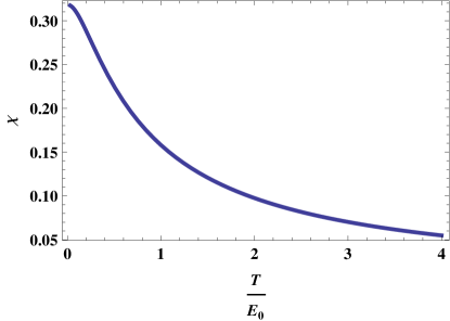
Figure 1: Temperature dependence of the magnetic susceptibility (24).

The spin sector contribution to the specific heat is

$$C=\frac{3T}{4\pi E_{0}}\int_{0}^{\infty}\frac{\mbox{d}xx^{2}}{[x^{2}(T/E_{0})^{2}+1]\cosh^{2}(x/2)}=\frac{3T}{4\pi E_{0}}\Big{[}1-\frac{E_{0}}{2\pi T}\psi^{\prime}\Big{(}E_{0}/2\pi T+1/2\Big{)}\Big{]}.$$ (26)

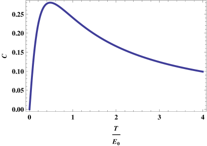
Figure 2: Temperature dependence of the spin sector contribution to the specific heat (26).

We see that at $T<<E_{0}$ the susceptibility is constant and the specific heat is linear in T. Hence at energies smaller than $E_{0}$ the impurity spin is fully screened.

II.1 Spin-orbit coupling

Our model (2) can be easily augmented by inclusion of the spin-orbit coupling:

$$H_{SO}=\Lambda{\bf T}{\bf S}.$$ (27)

At the 2-channel QCP we replace ${\bf T}$ as in (7) to get

$$H_{SO}\rightarrow\mbox{i}\frac{\Lambda}{\sqrt{T_{K}^{orb}}}\epsilon\chi^{a}S^{a}$$ (28)

This term combines with (10) such that now the impurity spin interacts with a linear combination of the orbital and spin Majoranas:

$$\cos\alpha\chi^{a}+\sin\alpha\xi^{a},~{}~{}\tan\alpha=g_{2}^{*}T_{K}^{orb}/\Lambda,$$ (29)

with the coupling constant

$$\tilde{V}=(\Lambda^{2}/T_{K}^{orb}+(g_{2}^{*})^{2}T_{K}^{orb})^{1/2}.$$ (30)

Thus, we see that the spin-orbit coupling does not bring any qualitative changes.

III A model with generic symmetry

As mentioned earlier, a single impurity version of model (1) is not solvable. However, it is still possible and worthwhile to make some qualitative statements about it. Consider model (1) with U(1)$\times$SU(N)$\times$SU(M) symmetry. An analog of decomposition (4) in this case is (see, for example, wznw ,wznw1 ,ludwig ):

$$\sum_{j=1}^{M}\sum_{\sigma=1}^{N}\sum_{k}\psi^{+}_{j\sigma}(k)(\partial_{\tau}-\epsilon_{k})\psi_{j\sigma}(k)=$$ (31)

$$\int_{-\infty}^{\infty}\mbox{d}x\partial_{x}\phi(\mbox{i}\partial_{\tau}+\partial_{x})\phi+\frac{2\pi}{N+M}\int\mbox{d}x\Big{[}:J^{a}J^{a}:+:F^{a}F^{a}:\Big{]},$$

where $J^{a}$ ($a=1,...N^{2}-1)$ and $F^{a}$ ($a=1,...M^{2}-1$) are currents from SU(N)_M and SU(M)_N Kac-Moody algebras defined as

$$J^{a}=\sum_{j=1}^{M}\psi^{+}_{j\alpha}\sigma^{a}_{\alpha\beta}\psi_{j\beta},~{}~{}F^{a}=\sum_{\sigma=1}^{N}\psi^{+}_{j\alpha}\tau^{a}_{jk}\psi_{k\alpha}$$ (32)

with $\sigma^{a},\tau^{a}$ being generators of the corresponding groups. For general $N\neq M$ the quadratic forms of currents cannot be expressed as models of free fermions as it happens for $N=M$, where they can be written in terms of Majorana fermions transforming in the adjoint representation of the SU(N) group. Neither does it work for the cross term in (2). Instead we have

$$\psi^{+}{\tau^{a}\sigma^{b}}\psi\rightarrow\Phi^{a}\Lambda^{b},$$ (33)

where $\Phi,\Lambda$ are Wess-Zumino primary fields from the adjoint representations of the SU(M) and SU(N) groups respectively. Their conformal dimensions are

$$h_{\Phi}=\frac{M}{N+M},~{}~{}h_{\Lambda}=\frac{N}{N+M}.$$ (34)

The QCP corresponds to the overscreening of the SU(N) sector. The corresponding Kondo scale is $T_{K}^{orb}=Wg_{1}^{M/N}\exp(-2\pi/Ng_{1})$. At the QCP one operator $\Phi$ creates an average with the impurity spin leaving behind a zero mode, fashioned along the lines of (7,10). As a result, the operator perturbing the critical SU_N(M) WZNW model is $\Lambda^{b}$ coupled to the SU(M) impurity spin. Its scaling dimension is $N/(N+M)<1$ and hence it is relevant. Thus, we can be confident that the model scales to strong coupling, which is presumably a Fermi liquid, but the details of this are not known. Consequently, the corresponding energy scale marking the crossover to Fermi liquid is

$$E_{0}\sim g_{2}^{1/(1-h_{\Lambda})}T_{K}^{orb}$$ (35)

IV Conclusion and Acknowledgements

We have presented an analytically tractable single impurity Kondo model where the impurity carries both spin and pseudospin $S=T$ =1/2 and the bulk electrons carry both spin and orbital indices. Our original motivation for considering this model was its relevance to the problem of ”bad” metals, as formulated in millis ,gabi ,piers . As we have already mentioned, according to DMFT, the single impurity problem describes both thermodynamics and the electron self energy within a range where the intersite correlations are relatively weak. Although the experimentally relevant models have different values of $S$, we have chosen $S=1/2$ to obtain analytic results.

Furthermore, we have considered the most interesting regime when the orbital moment is screened first and the coupling between spin and orbital channels is weak. Therefore, the screening of the orbital moment leads to a non-Fermi-liquid quantum critical point (QCP) which is destabilized by the interaction term mixing spin and orbital channels. If the corresponding coupling constant $g_{2}$ is small, there is a wide crossover regime between the unstable two-channel Kondo model QCP at high energies and coherent Fermi liquid at low energies. The ratio of these two energy scales is $\sim g_{2}^{2}$.

It is quite likely that the nonuniversal exponents in the self energy gabi discussed in the Introduction are crossover effects. To illustrate this point one needs to calculate the self energy; we plan to do it in a subsequent paper.

AMT is grateful to G. Kotliar, S. Lukyanov, R. M. Konik and P. Coleman for inspirational discussions and to A. James for help with the numerical calculations. The work was supported by the US DOE under contract number DE-AC02-98 CH 10886.

References

- (1) P. Werner, E. Gull, M. Troyer, and A. J. Millis, Phys. Rev. Lett. 101, 166405 (2008).
- (2) Z. P. Yin, K. Haule, G. Kotliar, Phys. Rev. B86, 239904(E) (2012).
- (3) T. T. Ong, P. Coleman, Phys. Rev. Lett. 108, 107201 (2012).
- (4) A. M. Tsvelick and P. B. Wiegmann, J. Phys. C15, 1707 (1982).
- (5) A. M. Tsvelik, ”Quantum Field Theory in Condensed Matter Physics”, Ch. 31,32; Cambridge University Press, 2003.
- (6) P. Di Francesco, P. Mathieu, D. Senechal, ”Conformal Field Theory”, Springer 1996.
- (7) J. M. Maldacena and A. W. W. Ludwig, Nucl. Phys. B506, 565 (1997).
- (8) P. Coleman, L. B. Ioffe and A. M. Tsvelik, Phys. Rev. B52, 6611 (1995).
- (9) A. M. Tsvelick, J. Phys. C18, 159 (1985).
- (10) From this point on our results differ from the ones of piers .
- (11) I. S. Gradshtein and I. M. Ryzhik, ”Table of Integrals, Series and Products”, sixth edition, 3.415 (4).
- (12) I. Affleck, A. W. W. Ludwig, Phys. Rev. B 48, 7297 (1993).