Control Explicit—Data Symbolic
Model Checking: An Introduction

Abstract

A comprehensive verification of parallel software imposes three crucial requirements on the procedure that implements it. Apart from accepting real code as program input and temporal formulae as specification input, the verification should be exhaustive, with respect to both control and data flows. This paper is concerned with the third requirement, proposing to combine explicit model checking to handle the control with symbolic set representations to handle the data. The combination of explicit and symbolic approaches is first investigated theoretically and we report the requirements on the symbolic representation and the changes to the model checking process the combination entails. The feasibility and efficiency of the combination is demonstrated on a case study using the DVE modelling language and we report a marked improvement in scalability compared to previous solutions. The results described in this paper show the potential to meet all three requirements for automatic verification in a single procedure combining explicit model checking with symbolic set representations.

1 Introduction

Specification of the intended behaviour of a computer system forms the basis of any rigorous, contract-based development. The final product must comply with its specification, and until it does, until all functional, safety and performance requirements are met, the development continues and the expenses grow. Requirements on safety and performance are rarely formalised, and thus compliance with those requirements is commonly ensured by strictly adhering to an established set of rules, e.g. DO-178B [19] for aviation systems. Functional requirements, on the other hand, often can be expressed in a precise, formal language – a property that makes them amenable to verification using formal methods.

Not all formal methods currently in practice, however, can handle requirements formalised in a language of sufficient expressivity. When programs behave nondeterministically, when they react to unpredictable environment or when the interleaving of components executed in parallel is unknown, the developers often need to express the desired behaviour as it evolves in time, using temporal logics [17]. Among the execution-based verification methods that exist, i.e. testing, symbolic execution [14] and model checking [9], only model checking is able to verify that a system is a model of the required temporal property [6].

Yet model checking in the present state is far from replacing testing and symbolic execution in real-world application. Apart from the well-known and well-understood problem of state space explosion, there are other aspects that prevent more widespread use. The one addressed by this paper is the restriction to closed systems, i.e. programs where each variable is initialised to a fixed value (see the related work for more detailed discussion of other attempts at model checking of open systems). Symbolic execution is not limited to closed systems; there the values of variables are represented symbolically, which in theory enables all possible values to be considered within a single run of such execution.

It seems that unifying these two formal methods, symbolic execution to gain access to open systems and model checking for temporal properties, could lead to a method of high practical value. Indeed, for carrying out unit tests [20] on a nondeterministic component within a larger program, neither technique alone would suffice to achieve substantial reliability of the product. Our approach to this unification is to augment the model checking by allowing to verify the correctness for multiple variable evaluations at a time. To represent the state space explicitly, but with the states being in fact symbolic sets of states: hence control explicit—data symbolic model checking.

A straightforward way for supporting open variables is to repeat the verification, as many times as there are combinations of the input values. It requires only a very small change in the implementation, as was demonstrated in [2], where the model checking was suitably modified for verification of Simulink circuits. When generating successors of a circuit state, the process first takes into consideration the branching in the specification transition system and then the branching in the program transition system (the control-flow branching). Resolution of the data-flow branching (caused by open input variables) can be attached to that of control-flow or, since Simulink circuits are otherwise deterministic, replace it. In other words, the states of the circuit model are treated as if having one successor for every combination of the input variable evaluations.

Needless to say, this approach is extremely demanding with respect to computational resources. Apart from the original (often merely potential) explosion caused by control-flow nondeterminism there is now an addition, inescapable explosion of data. Every variable multiplies the number of successors of every state by the size of its range. Even if the circuit only used Boolean variables, or equivalently if the range was always equal to two, the blow-up would still be exponential. For explicit model checking especially, such an approach is an interesting proof of concept, baseline for future improvements, but limited in application to academic examples and experiments. For use in practice, e.g. in industry-level unit testing, a cleverer approach needs to be adopted.

Contribution

On the most fundamental level, the modification of explicit model checking proposed in this paper lies in replacing the exponential number of states in the transition system with more complex successor generation. Model checking systems with input variables, i.e. with nontrivial data flow, entails either further state space explosion or employing some form of symbolic representation. Throughout this paper, we propose representing symbolically only the data part; the control part remains explicit. Not every symbolic representation, however, can be used and we detail as to what requirements must the representation meet to enable model checking against temporal properties. Using a basic representation that meets the proposed requirements, we have described how the model checking process must be modified to represent data symbolically. The experiments on Peterson’s communication protocol report far better scalability compared to the purely explicit approach. Replacing one level of the state space explosion for complex symbolic states and for the additional difficulty associated with their generation appears to have the potential to forward the progress towards practical verification of concurrent systems.

1.1 Related Work

Of the plethora of papers pertaining to execution-based verification only a few are directly related to the presented work. Firstly, there is the symbolic execution and the related research aiming at improving its robustness. For example, support for parallel or otherwise nondeterministically behaving systems was first incorporated in [13]. Allowing specification in LTL was partially introduced in [6], yet the undecidability of state matching limited the approach to only a small subset of LTL. The research that perhaps most closely resembles ours was described in a section on Delayed Nondeterminism in a PhD Thesis by Schlich [21]. There the variables were represented symbolically until used and then the algorithm opted for the explicit representation.

Symbolic model checking is most commonly applied on Boolean programs, avoiding many of the mentioned problems, especially those related to arithmetic. Computing multiplication with the standard representation, Binary Decision Diagrams [18], is exponential in the size of the representation [7]. Other representation were designed to remedy this deficiency, such as Binary Moment Diagrams [8] or Boolean Expression Diagrams [24]. These represent variables on the word level rather then on the binary level. Another direction of research attempted to utilise the advance of modern satisfiability solvers, first with classical SAT [4] and then with the more specific SMT [1]. However, SAT-based model checkers allow the state space to be traversed only to a bounded depth, which renders such model checking incomplete. It was also suggested to limit the scope of the symbolic model checking to programs with only Presburger arithmetics, where more efficient representation were applicable, e.g. Periodic Sets [5].

Various combinations of different approaches and representations have been devised and experimented with. When multiple representation were combined, it was mostly to improve on weak aspects of either of the representations, for example in [26] multiple symbolic representation for Boolean and integer variables were employed in combination. Finally, the two approaches to model checking, explicit and symbolic, were combined to improve solely upon control-flow nondeterminism. Some improvement was achieved by storing multiple explicit states in a single symbolic state [10] or by storing explicitly the property and symbolically the system description [22].

Our stating that model checking is restricted to closed systems requires further discussion. Module checking, introduced in [15] and detailed in [11], allows verification of open systems, though the meaning of openness differs from ours. The two sources of nondeterminism in module checking are internal and external, where the external nondeterminism is controlled by the environment. A system is open in the sense that the environment may restrict the nondeterminism and the verification has to be robust with respect to arbitrary restriction. The approach to verifying open systems also differs since only branching time logics can distinguish open from closed systems, in the module checking sense. For linear time logics, every path has to satisfy the property and thus open and closed systems collapse into one source of nondeterminism; where this paper intends to separate the nondeterministic choices emerging from control and data flows.

Much closer to our separation between control and data is the work initiated by Lin [16]. Lin’s Symbolic Transition Graphs with Assignments represent precisely parallel programs with input variables using a combination of first-order logic and process algebra for communicating systems. Similarly as for symbolic execution, the most complicated aspect of this representation is the handling of loops. Lin’s solution computes the greatest fix point of a predicate system representing the first-order term for each loop. Then two transition graph are bisimilar if the predicate systems representing all loops are equivalent. While the theoretical aspects of our work are very similar to Lin’s it is not clear how his equality of predicate systems could be used in LTL model checking, though it is intended as one of our future directions in research.

Finally, our work can be seen as an alternative approach to that described in [12]. There the authors also divide parallel programs into control and data, where control is handled using symbolic model checking and data by purely symbolic manipulation of first-order formulae. Avoiding the problems with loop – which were the main objective of Lin’s work – by not allowing symbolic data to influence control, the authors of [12] implemented verification of parallel programs against first-order branching logic. Hence while their distinction between control and data is almost precisely equivalent to ours, the method proposed in this paper allows verification against linear time logic with no restriction on the parallel program. The loops still pose a considerable problem, but can only severely increase the running time; they never render the verification task undecidable.

2 Preliminaries

The methodology proposed in this paper depends on various technical aspects of explicit model checking and specific input languages. These must be at least generally described for the purpose of further discussion. Within this section we will proceed from the more theoretical to more practical, from the foundations of model checking to its implementation.

Definition 1

Let $\Sigma$ be the set of atomic propositions. Then this recursive definition specifies all well-formed LTL formulae over $\Sigma$, where $p\in\Sigma$:

$\Psi::=p\mid\neg\Psi\mid\Psi\wedge\Psi\mid X\ \Psi\mid\Psi\ U\ \Psi$

Example 1

There are some well-established syntactic simplifications of the LTL language, e.g. $\mathit{false}:=p\wedge\neg p$, $\mathit{true}:=\neg\mathit{false}$, $\phi\Rightarrow\psi:=\neg(\phi\wedge\neg\psi)$, $F\ \phi:=$ $\mathit{true}\ U\ \phi$, $G\ \phi:=\neg(F\ \neg\phi)$. Assuming that $\Sigma=\{\alpha:=(c=5),\beta:=(a\neq b)\}$, these are examples of well-formed LTL formulae: $G\ \beta,\alpha\ U\ \neg\beta$. Informally, the first one states that $a$ must never be equal to $b$ and the second that $c$ is equal to $5$ as long as $a$ equals $b$ (and at some point $a$ must become different from $b$). $\triangle$

Definition 2

A Labelled Transition System (LTS) $M=(S,\rightarrow,\nu,s_{0})$ is a tuple, where: $S$ is a set of states, $\rightarrow\subseteq S\times S$ is a transition relation, $\nu:S\rightarrow 2^{\Sigma}$ is a valuation function and $s_{0}\in S$ is the initial state. A function $r:\mathbb{N}\rightarrow S$ is an infinite run over the states of $M$ if $r(0)=s_{0},\forall i:r(i)\rightarrow r(i+1)$. The trace or word of a run is a function $w:\mathbb{N}\rightarrow 2^{\Sigma}$, where $w(i)=\nu(r(i))$.

Traversing an LTS requires the underlying graph to be represented, in some form, in the computer memory. There are two categories of suitable graph representations: explicit, where vertices and edges are already stored in the memory and implicit, where successors are generated on-the-fly from the description of their predecessors. For implicit representation, only two functions must be provided as the system description: initial state to generate the initial system configuration and successors. The latter function takes as the input a single state and, based on the control-flow choices available in that state, returns the set of successor states of the input state.

An LTL formula states a property pertaining to an infinite trace; see how traces relate to runs in Definition 2. Assuming the LTS is a model of a computer program then a trace represents one specific execution of the program. Also the infiniteness of the executions is not necessarily an error – programs such as operating systems or controlling protocols are not supposed to terminate (and indeed would be incorrect if they did terminate).

Definition 3

Let $w$ be an infinite word and let $\Psi$ be an LTL formula over $\Sigma$. Then the following rules decide if $w$ satisfies $\Psi$, $w\models\Psi$, where $w(i)$ is the $i$-th letter of $w$ and $w_{i}$ is the $i$-th suffix of $w$:

$$\begin{array}[]{lcl}w\models p&\ \mathit{iff}&\ p\in w(0),\\ w\models\neg\Psi&\ \mathit{iff}&\ w\not\models\Psi,\\ w\models\Psi_{1}\wedge\Psi_{2}&\ \mathit{iff}&\ w\models\Psi_{1}\ \mathit{and}\ w\models\Psi_{2},\\ w\models X\ \Psi&\ \mathit{iff}&\ w_{1}\models\Psi,\\ w\models\Psi_{1}\ U\ \Psi_{2}&\ \mathit{iff}&\ \exists i\forall j<i:w_{j}\models\Psi_{1},w_{i}\models\Psi_{2}.\end{array}$$

Clearly, a system as a whole satisfies an LTL formula if all its executions (all infinite words over the states of its LTS) do. Efficient verification of that satisfaction, however, requires a more systematic approach than enumeration of all executions. An example of a successful approach is the enumerative approach using Büchi automata.

Definition 4

A Büchi automaton is a tuple $A=(S,\rightarrow,\nu,s_{0},F)$, formed of an LTS $M=(S,\rightarrow,\nu,s_{0})$ and $F\subseteq S$. An automaton $A$ accepts an infinite word $w$, $w\in L(A)$, if there exists a run $r$ for $w$ in $M$ and there is a state from $F$ that appears infinitely often on $r$, i.e. $\forall i\exists j>i:r(j)\in F$.

Arbitrary LTL formula $\phi$ can be transformed into a Büchi automaton $A_{\phi}$ such that $w\models\phi\Leftrightarrow w\in L(A_{\phi})$. Also checking that every execution satisfies $\phi$ is equivalent to checking that no execution satisfies $\neg\phi$. It only remains to combine the LTS model of the given system $M$ with $A_{\neg\phi}$ in such a way that the resulting automaton will accept exactly those words of $M$ that violate $\phi$. Finally, deciding existence of such a word – and by extension verifying correctness of the system – is equivalent to detecting accepting cycle in the underlying graph [9].

Returning back to the implementation of the model checking process, already having the initial state and successors functions, the description can be finalised by adding one more function: is accepting. With this function, which returns a binary answer when provided with an LTS state, one can represent Büchi automata and consequently detect accepting cycles within.

That is, however, a significant step and not entirely a trivial one. A state of the product LTS comprises two states, one for the specification and one for the system. It follows that the successors function must also be modified, because now there are control choices also from the specification LTS. These control choices are based on whether or not particular atomic propositions hold in the input state, such that the property remains satisfied. The described modifications are sufficient for LTL model checking, assuming, and that is an aspect of major importance for this paper, that the states of the product LTS are stored and that duplicates in the state space can be detected. The basis for this importance will become apparent in the next chapter.

3 Explicit Control with Symbolic Data

Automata-based model checking, as presented in the previous section, handles only control-flow nondeterminism. That would be perfectly sufficient if communication protocols were the only type of input models, but should model checking aspire to verify correctness of real software, such limitation would decrease its usability. Small units of programs often take inputs and possible values of these inputs – each defining a new, potentially unique execution – must be considered as well; otherwise the verification would not be exhaustive.

Handling of both sources of nondeterminism combined within a single procedure is a logical next step when adapting model checking for the use in unit testing. This paper proposes allowing the specification of ranges of the input variables in verified programs, i.e. allowing verification with open variables, even though bounded. Two approaches for handling such modification present themselves. Firstly, simply run one instance of the model checking process for every combination of the input variables: an approach described in Section 1. Secondly, and what is devised in this paper, run model checking only once but instead of simple, single-value states use multi-states encoding multiple values of variables.

3.1 Set-Based Reduction

The states of computation in a parallel program are uniquely defined by the evaluation of variables and the program counters of individual threads. Other program components needed for execution, such as stack and heap contents, are assumed to be represented as fresh variables. Given this abstraction we can define a transition system generated by the execution of a parallel program in exactly the same manner as in Definition 2. For the purposes of distinguishing the two sources of nondeterminism, control and data, we will associate with a parallel program $P$, a transition system $\mathcal{T}^{P}=(S,\rightarrow,\nu,S_{0})$, where each $s\in S$ is composed of two parts $s=(s_{c},s_{d})$. (Also $S_{0}$ is a subset of $S$, since there generally are many initial evaluations.) There $s_{c}$ represents the evaluation of program counters and other variables that are not modified externally and $s_{d}$ represents the evaluation of input variables. Similar state composition is preserved when the product with a Büchi automaton is computed, i.e. given a program $P$ and a Büchi automaton $A_{\varphi}$, the states of the product $\mathcal{A}^{P}_{\varphi}$ are again composed of two parts, where the information identifying the states of $A_{\varphi}$ is part of $s_{c}$.

Figure 1: Example verification task: for a program $P$ and a specification $\varphi$, the verification traverses the transition system $\mathcal{A}^{P}_{\varphi}$.

Example 2

Consider the verification task depicted in Figure 1. The identification of program states can be divided into two parts: one for control information (marked with lighter blue in the figure) and the other for data (marked with darker red). Note also that the control part contains the program counters for individual threads of the main program and the states $\varphi$ of the specification automaton $\mathcal{A}_{\varphi}$. Similarly, it is possible to distinguish the two sources of nondeterminism in parallel programs: the control-flow nondeterminism (thread interleaving) is marked as $\zeta$-transitions and the data-flow nondeterminism (variable evaluation) as $\delta$-transitions. $\triangle$

Note that the state space of this transition system is exponential both in the number of parallel threads and in the number of input variables. This paper attempts to partly remedy the second state space explosion caused by the data flow by introducing a set-based reduction. Intuitively, the reduction unifies those states that (1) have the same control part and at the same time (2) the possible evaluation of their data parts form the same sets. Formally, we can define the reduced state space inductively, starting from the initial states $S_{0}=\{s^{1},s^{2},\ldots,s^{n}\}$, where $s^{i}=(s^{i}_{c},s^{i}_{d})$ and $\forall i,j:s^{i}_{c}=s^{j}_{c}=s_{c}$. Then the one initial multi-states of the set-reduced transition system $\mathcal{T}_{set}=(\mathfrak{S},\rightarrow,\nu^{\prime},\mathfrak{s}_{0})$ is $\mathfrak{s}_{0}=(s_{c},\{s^{i}_{d}|i\leq n\})$. For a state $\mathfrak{s}=(s_{c},\{x_{1},\ldots,x_{n}\})$ let $\mathsf{S}=\{s|\exists i:(s_{c},x_{i})\rightarrow s\}$ be the set of successors in the unreduced state space and $\nu^{\prime}:\mathfrak{S}\rightarrow 2^{\Sigma}$ have $\nu^{\prime}(\mathfrak{s})=\bigcup_{i=1}^{n}\nu(s_{c},x_{i})$. Then the successors of $\mathfrak{s}$ in $\mathcal{T}_{set}$ form a set $\{(s,X)|x\in X\Leftrightarrow(s,x)\in\mathsf{S}\}$.

The reduced transition system can be combined with a Büchi automaton in a similar fashion as the unreduced state space. The resulting automaton $\mathcal{A}_{set}=(\mathfrak{S},\rightarrow,\nu^{\prime},s_{0},F^{\prime})$, where $F^{\prime}\subseteq\mathfrak{S}$ has the property that the set of accepting multi-states respects the accepting states of the unreduced automaton. Formally, let $F_{\exists},F_{\forall}\subseteq\mathfrak{S}$ such that $(s_{c},X)\in F_{\exists}\Leftrightarrow\exists x\in X:(s_{c},x)\in F$ and $(s_{c},X)\in F_{\forall}\Leftrightarrow\forall x\in X:(s_{c},x)\in F$. Then it holds that $F_{\exists}=F_{\forall}$ and thus either can be used to define $F^{\prime}$. The reason for this property of the proposed reduction is that the state of the Büchi automaton used in the product is contained in the control part of both states and multi-states, and hence remains unreduced. Detailed reasoning would be rather technical and the reader need only realise that while $\nu$ might evaluate some atomic propositions differently on states within a single multi-state, the atomic propositions used in $\varphi$ must be evaluated consistently within a multi-state. Otherwise the respective multi-states would be split when generating successors.

Example 3

There are two programs that nicely exemplify some of the properties of set-based reduction, which we will use in further discussion, especially regarding the efficiency. Consider the following program with a loop:
cin >> a; while ( a > 10 ) a--;
When only the data part of multi-states is considered, the reduced transition system unfolds to

and while the state space is finite, there are as many multi-states in the reduction system as there were states in the original system. Furthermore, many states are represented multiple times: given that the first and the third states in the above system have the same program counter, the values of $a$ between 10 and 254 are represented twice in these two multi-states alone.

On the other hand, for a specification and a program
x = 1; cin >> y; while ( true ) y++;
the reduced transition system contains three multi-states and three transitions:
whereas the original transition system contains 256 path that each enclose into a cycle only after 256 unfoldings of the while loop. $\triangle$

The set-based reduction preserves the properties of the original transition system with respect to LTL model checking as the following theorem shows. Thus a standard model checking procedure as described in Section 2 can be used to verify correctness of a parallel program with respect to an LTL property.

Theorem 3.1 (Correctness)

The product $\mathcal{A}=(S,\rightarrow,\nu,S_{0},F)$ of a program transition system $\mathcal{T}$ and a Büchi automaton $A$ contains an accepting cycle iff there exists one in the reduced $\mathcal{A}_{set}=(\mathfrak{S},\rightarrow,\nu^{\prime},\mathfrak{s}_{0},F^{\prime})$.

Proof

$\Rightarrow$ Let $\leadsto$ be the reflective and transitive closure of $\rightarrow$. Also for any $t=(t_{c},t_{d})\in S$ and $\mathfrak{s}=(s_{c},X)\in\mathfrak{S}$, let $t\sqsubseteq\mathfrak{s}$ iff $t_{c}=s_{c}\wedge t_{d}\in X\wedge\nu(t)\subseteq\nu^{\prime}(\mathfrak{s})\wedge$ $t\in F\Leftrightarrow\mathfrak{s}\in F^{\prime}$. One might observe that for any path $s_{1}\rightarrow s_{2}\rightarrow\ldots\rightarrow s_{n}$ in $\mathcal{A}$ there is a path $\mathfrak{s}_{1}\rightarrow\mathfrak{s}_{2}\ldots\rightarrow\mathfrak{s}_{n}$ in $\mathcal{A}_{set}$ such that for all states along the path it holds that $s_{i}\sqsubseteq\mathfrak{s}_{i}$. Assume $t_{0}\leadsto t_{1}\rightarrow\ldots\rightarrow t_{n}=t_{1}$ in $\mathcal{A}$ and hence also $\mathfrak{t}_{0}\leadsto\mathfrak{t}_{1}\rightarrow\ldots\rightarrow\mathfrak{t}_{n}$ in $\mathcal{A}_{set}$. But it the reduced state space it might happen that $\mathfrak{t}_{n}\neq\mathfrak{t}_{1}$ but instead $\mathfrak{t}_{n}=\mathfrak{t}^{\prime}_{1}$. Unrolling the cycle in $\mathcal{A}$ further we get $\mathfrak{t}_{1}\leadsto\mathfrak{t}^{\prime}_{1}\leadsto\mathfrak{t}^{\prime\prime}_{1}\leadsto\ldots$ in $\mathcal{A}_{set}$. Yet if $\mathfrak{t}=(t_{c},X)$ then $t_{c1}=t^{\prime}_{c1}=\ldots$ and also $X_{1}\supseteq X^{\prime}_{1}\supseteq\ldots$. To understand why the second part of the previous statement holds one needs only to remember that given $t_{1}=t_{n}$ the combined effect of the program between $t_{1}$ and $t_{n}$ on the data part has to be an identity. $X_{1},X^{\prime}_{1},\ldots$ may not be equal only because the program conditions along the path further limit what values of input variables might have led to this state of computation. It immediately follows that the sequence $X_{1},X^{\prime}_{1},\ldots$ has a fix point $\mathfrak{t}^{m}_{1}$, which is the first multi-state of a cycle in $\mathcal{A}_{set}$. Finally, since the relevant path in $\mathcal{P}$ may be arbitrarily unrolled along the cycle $t_{1}\leadsto t_{1}$, it still holds that for $t_{0}\leadsto t_{1}(\leadsto t_{1})^{m}\leadsto t_{1}$ and $\mathfrak{t}_{0}\leadsto\mathfrak{t}^{m}_{1}\leadsto\mathfrak{t}^{m}_{1}$ $t\sqsubseteq\mathfrak{t}$ along the paths and thus the cycle $\mathfrak{t}^{m}_{1}\leadsto\mathfrak{t}^{m}_{1}$ is accepting in $\mathcal{A}_{set}$.

$\Leftarrow$ Assume $\mathfrak{t}_{0}\leadsto\mathfrak{t}_{1}\rightarrow\ldots\rightarrow\mathfrak{t}_{n}=\mathfrak{t}_{1}$ in $\mathcal{A}_{set}$. Then as above there must be a path $t_{0}\leadsto t_{1}\rightarrow\ldots\rightarrow t_{n}$ in $\mathcal{A}$ such that $t\sqsubseteq\mathfrak{t}$ all along the path but again $t_{1}$ may not be equal to $t_{n}=t^{\prime}_{1}$. Let $t_{1}=(t_{c1},t_{d1})$ and let $\kappa$ be the operation applied on $t_{d1}$, i.e. $t^{\prime}_{d1}=\kappa(t_{d1})$, then $t^{\prime}_{c1}=t^{\prime\prime}_{c1}=\ldots$ and we will show that there exists $m$ such that $\kappa^{m}(t_{d1})=t_{d1}$. It follows from the fact that the underlying structure of the data part is a commutative ring $\mathbb{Z}/k\mathbb{Z}$ of integers modulo $k$, where $k$ is the product of the domains of input variables. Computer programs use modular arithmetic and it is a property of such arithmetic that for any operation $\kappa$ there is an $m$ such $m$ iterations of $\kappa$ is an identity. The rest of this implication is similar to the previous one.∎

As apparent from Example 3, reasoning about the efficient of the proposed set-based reduction – the ratio between the size of the original system and the size of the reduced system – is rather complicated. For a program without cycles, the reduction is exponential with respect to the number of input variables and to the sizes of their domains. Note, however, that for trivial cases of data-flow nondeterminism even this reduction can be negligible. The case of programs with cycles is considerably more involved.

Let us call cycles those paths in a transition system that start and end in two states with the same control part, $s=(s_{c},s_{d})$ and $s^{\prime}=(s_{c},s_{d}^{\prime})$. Then the function $f$ of the cycle, transforming $s_{d}$ to $s_{d}^{\prime}$, has a fix point as was argued in the above proof, and this fix point has to be computed (explicitly in our case, as opposed to symbolic solution [16] of the same problem). That aspect is present in full and reduced state spaces alike, yet may produce an exponential difference in their sizes. If the multi-state already contains the fix point before it reaches given cycle, as in the second program of Example 3, then the reduced system contains only as many multi-states as is the length of that cycle. On the other hand, as the first program of Example 3 demonstrated, the reduction can even be to the detriment of the space complexity even if we assume that the size of multi-states is sublinear in the number of states contained within, which is difficult to achieve, as we discuss in the conclusion.

The remainder of this section will investigate the necessary properties the hybrid representation must possess to enable LTL model checking by following the steps forming the model checking process and describing how each must be altered. As described in Section 2, LTL model checking requires implementation of three functions: initial state, successors, and is accepting.

3.2 Changes in LTS Traversal

Initial Ranges

The multi-states, as mentioned above, consist of two parts, but unless it proves to impede the clarity we will assume only the symbolic part to be present. Under this assumption the initial state function returns a set of every combination within the initial ranges of the undefined variables. For example, in case of two variables $a\in\{1,\ldots,5\}$, and $b\in\{4,\ldots,5\}$, the initial multi-state represents a set $\{(a,b)|1\leq a\leq 5\wedge 4\leq b\leq 5\}$.

Assignments and Conditions

Generating successors must take into consideration the branching of control flow and must allow changing the evaluation of variables. Without the loss of generality one can expect the successors to use only two methods to interact with variables: prune and apply. prune takes a Boolean expression $e$, evaluates it and removes all evaluations in the multi-state that do not satisfy $e$. apply takes an assignment, a pair (variable $v$, expression $e$) and updates the evaluation accordingly. Applying an assignment on a multi-state entails considering every combination of stored values, evaluating $e$ on that combination and finally updating $v$ for the value of $e$. Conditional branching is handled by prune and assignments are handled by apply. Which leaves only cycles.

Decidable Equality

Dealing with cycles represents a major problem for execution-based verification. They are either unwound [6], which is imprecise, or considered naively, which leads to infinite state spaces [13]. Our insisting on having LTL specifications, however, has one very specific consequence when dealing with cycles. Accepting cycle detection algorithms require duplicate detection to be decidable, i.e. the representation must enable checking equality of multi-states. Hence every multi-state is stored only once and consequently, the state space must be finite, even with cycles in the LTS.

It might appear that differentiating every two multi-state that only differ in their data parts produces unnecessarily too large state spaces; that subsumption [25] could be a sufficient condition for state equality. That is not correct with respect to LTL. For a state $S$ assume that a different state $S^{\prime}$ is found such that $S^{\prime}\subseteq S$. If these were matched into a single state $S$ and there was a path from $S^{\prime}$ to $S^{\prime\prime}\subseteq S$ such that $S^{\prime\prime}\cap S^{\prime}=\emptyset$, then the reduced transition system would contain a cycle where there was none in the original system.

3.3 Changes in Counterexample Computation

Pruning when generating successors leads to complications because the current multi-state is implicitly divided, based on which of its evaluations satisfy given condition. However, the information necessary for such division is only available when the successors are generated, i.e. after the actual source multi-state was stored. Only with hindsight can one express what evaluation of the input variables leads to a certain state.

This unintended consequence does not affect the model checking procedure itself, but it affects its crucial part: the counterexample generation. A counterexample represents the path that leads to an accepting cycle – the piece of information that specifies the defect of the system under verification. Standard explicit model checking generates counterexamples by traversing the LTS backwards from the accepting cycle along the so-called parent graph, a tree generated during the forward traversal. To remedy this consequence of using multi-states, it suffices (during the backwards traversal) to prune the multi-state to contain only the correct evaluations. An example: at some point the backwards traversal follows a transition that leads to a multi-state, which, in order to follow the transition in forward traversal, must satisfy $a>5$. Then those evaluations for which $a\leq 5$ are removed from this multi-state. Note also that this approach is robust even to accommodate the reduced cycle of the second program in Example 3.

4 Case Study

In this introductory paper we aim at validating the proposed method and use explicit sets to represent multi-states. There still are space reductions, considerable as will be demonstrated in the experiments, resulting from the redundancy exhibited by the repeated execution. The evaluation of defined variables and control-flow information, e.g. the program counter, was stored in every state, once for every evaluation of undefined variables. Now it is only stored once, as the explicit part of a multi-state. The space reductions would be undeniably greater have we used a symbolic representation of sets. However, as mentioned before, LTL specification is paramount to us, equality of multi-states must be decidable – a property which many symbolic representations lack.

4.1 The DVE Language

The DVE language was established specifically for the design of protocols for communicating systems. There are three basic modelling structures in DVE: processes, states, and transitions. At any given point of time, every process is in one of its states and a change in the system is caused by following a transition from one state to another. Communication between processes is facilitated by global variables or channels, that connect two transitions of different processes: the two transitions are followed concurrently. Following a transition is conditioned by guard expressions, that the source state must satisfy, and entails effects, an assignment modifying the variable evaluation. LTL specification is merely another process, whose transitions are always connected to the system transitions. Comprehensive treatment of the DVE syntax and semantics can be found in [23].

The DVE language allows using variables of different types and consequently of different sizes and, thus, the proposed modification only adds the specification which variables are undefined and what are their ranges. States are represented as an evaluation of variables and a map assigning a state to each process. In multi-states, the original states are preserved as the explicit part and the symbolic part is a representation of the undefined variables (stored as a new, defined variable in the explicit part). Once restored from memory, the explicit evaluation of variables forms the so-called context.

When following a transitions, the function successors calls the method prune with a guard as its parameter. If the representation results in being empty, i.e. not a single evaluation satisfies the guard, then no successors are generated. Otherwise, the effect is applied and the resulting representation is stored in a new multi-state. The evaluation of expressions is undertaken in a standard way, except that every combination of undefined variables is first loaded into the context: there is no need to modify the underlying arithmetic.

4.2 Experiments

The above described case study for the DVE language was implemented  in the DiVinE [3] verification environment, which already supported the DVE input language for system description. The change consisted only of the addition of hybrid representation, and by extension of support for partially open systems. The model checker remained unmodified, the parallel accepting cycle detection algorithms and specialised data structures could still be used without additional alternation of the code. Similar conditions were chosen for the comparison between repeated execution (unmodified DiVinE) and the new hybrid approach: the codes were compiled with optimisation option -O2 using GCC version 4.7.2 and ran on a dedicated Linux workstation with 64 core Intel Xeon 7560 @ 2.27GHz and 512GB RAM.

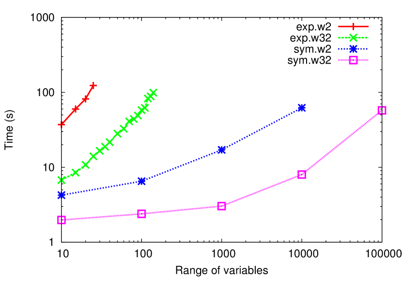
(a) Time complexity for peterson-liveness

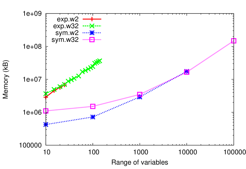
(b) Space complexity for peterson-liveness

We have conducted a set of experiments pertaining to the Peterson’s communication protocol. For the purposes of verification, the protocol is usually modelled in such a way that once a process accesses the critical section, it immediately leaves the critical section, without performing any work. The introduction of input variables allows the model to achieve closer approximation of practical use by simulating some action in the critical section, however artificial that action might be. Hence a global input variable $l\in\{0\ldots\mathsf{r}\}$ was added to the model and an action $l=(l+1)\%\mathsf{r}$. Note that the action is not biased towards set-based reduction because it forces inclusion of all subsets $\{0\ldots\mathsf{r}\},\{1\ldots\mathsf{r}\},\ldots$ even in the reduced state space.

The two plots above report the results of liveness verification of this modified Peterson’s protocol. Verification of this protocol is nontrivial and the best parallel algorithm OWCTY (see [3] for more details of this and other parallel algorithms used in DiVinE) requires several iteration before it can answer the verification query. The experiments were executed using the fully explicit approach of [2], denoted as exp, and the hybrid approach proposed in this paper, denoted as sym; using 2 and 32 parallel threads (w2 and w32). The plots clearly show that the fully explicit approach cannot scale with the range of input variables $r$ (the $x$-axis) and even when 32 parallel threads were used, verification of a single variable of range $0..140$ required almost 100 seconds. Our hybrid approach scaled markedly better, easily achieving the range up to 10000 with the same spacial complexity that exp needed for two orders of magnitude smaller range.

5 Conclusion

This paper represents an initial step towards complete and precise verification of parallel software against temporal specification. We investigate the potential of the combination of explicit and symbolic approaches, handling the control-flow explicitly and the data-flow symbolically, as the mean of taking this step. The potential is demonstrated in the preliminary results, on the experiments conducted with a communication protocol and a trivial explicit set representation, where the scalability of combining explicit and symbolic approaches surpasses the purely explicit approach. Even with the most basic symbolic representation for data, we have multiplied the allowed range of input variables. The data domain is still bounded, but that is a reasonable price to pay for temporal specification: one only needs to expand the boundary from $0$–$n$ to $0$–$2^{n}$.

Moving from a linear bound to a logarithmic bound on data is the long-term goal of our research. Purely symbolic representations (BDDs and similar) might allow such a move, but these are limited as to what operations on the data the representations support. More immediate possibilities lie in relaxing some of the imposed limitations, e.g. supporting only Presburger arithmetic would still allow precise verification on logarithmically bounded variables, while retaining the ability to verify against temporal specification. The first-order theory of bit-vectors appears most promising; there the greatest challenge would be the methodology of comparing two multi-states and the ranges of input variables much manageable problem.

References

- [1] A. Armando, J. Mantovani, and L. Platania. Bounded Model Checking of Software Using SMT Solvers Instead of SAT Solvers. In SPIN, volume 3925 of LNCS, pages 146–162. Springer, 2006.
- [2] J. Barnat, J. Beran, L. Brim, T. Kratochvíla, and P. Ročkai. Tool Chain to Support Automated Formal Verification of Avionics Simulink Designs. In FMICS, volume 7437 of LNCS, pages 78–92. Springer, 2012.
- [3] J. Barnat, L. Brim, V. Havel, J. Havlíček, J. Kriho, M. Lenčo, P. Ročkai, V. Štill, and J. Weiser. DiVinE 3.0 – Explicit-state Model-checker for Multithreaded C/C++ Programs. In To appear in Proc. of CAV, 2013.
- [4] A. Biere, A. Cimatti, E. Clarke, M. Fujita, and Y. Zhu. Symbolic Model Checking Using SAT Procedures instead of BDDs. In Proc. of DAC, pages 317–320, 1999.
- [5] B. Boigelot and P. Wolper. Symbolic Verification with Periodic Sets. In CAV, volume 818 of LNCS, pages 55–67. Springer, 1994.
- [6] P. Braione, G. Denaro, B. Křena, and M. Pezzè. Verifying LTL Properties of Bytecode with Symbolic Execution. In Proc. of Bytecode, 2008.
- [7] R. Bryant. On the Complexity of VLSI Implementations and Graph Representations of Boolean Functions with Application to Integer Multiplication. IEEE Trans. Comput., 40(2):205–213, 1991.
- [8] R. Bryant and Y.-A. Chen. Verification of Arithmetic Circuits with Binary Moment Diagrams. In Proc. of DAC, pages 535–541, 1995.
- [9] E. Clarke, E. Emerson, and A. Sistla. Automatic Verification of Finite-State Concurrent Systems Using Temporal Logic Specifications. ACM T. Progr. Lang. Sys., 8(2):244–263, 1986.
- [10] A. Duret-Lutz, K. Klai, D. Poitrenaud, and Y. Thierry-Mieg. Self-Loop Aggregation Product — A New Hybrid Approach to On-the-Fly LTL Model Checking. In ATVA, volume 6996 of LNCS, pages 336–350. Springer, 2011.
- [11] P. Godefroid. Reasoning about Abstract Open Systems with Generalized Module Checking. In EMSOFT, volume 2855 of LNCS, pages 223–240. Springer, 2003.
- [12] H. Hungar, O. Grumberg, and W. Damm. What if Model Checking Must Be Truly Symbolic. In CHARME, volume 987 of LNCS, pages 1–20. Springer, 1995.
- [13] S. Khurshid, C. Păsăreanu, and W. Visser. Generalized Symbolic Execution for Model Checking and Testing. In TACAS, volume 2619 of LNCS, pages 553–568. Springer, 2003.
- [14] J. King. Symbolic Execution and Program Testing. Commun. ACM, 19(7):385–394, 1976.
- [15] O. Kupferman and M. Vardi. Module Checking. In CAV, volume 1102 of LNCS, pages 75–86. Springer, 1996.
- [16] H. Lin. Symbolic Transition Graph with Assignment. In CONCUR, volume 1119 of LNCS, pages 50–65. Springer, 1996.
- [17] Z. Manna and A. Pnueli. Verification of Concurrent Programs, Part I: The Temporal Framework. Technical report, Stanford University, 1981.
- [18] K. McMillan. Symbolic Model Checking. PhD thesis, Carnegie Mellon University, 1992.
- [19] RCTA. DO-178-B, Software Consideratons in Airborne Systems and Equipment Certification. Technical report, RCTA, 1992. 548-92/SC167-177.
- [20] P. Runeson. A Survey of Unit Testing Practices. IEEE Software, 23(4):22–29, 2006.
- [21] B. Schlich. Model Checking of Software for Microcontrollers. PhD thesis, Aachen University, 2008.
- [22] R. Sebastiani, S. Tonetta, and M. Vardi. Symbolic Systems, Explicit Properties: On Hybrid Approaches for LTL Symbolic Model Checking. In CAV, volume 3576 of LNCS, pages 100–246. Springer, 2005.
- [23] P. Šimeček. DiVinE – Distributed Verification Environment. Master’s thesis, Masaryk University, 2006.
- [24] P. Williams, A. Biere, E. Clarke, and A. Gupta. Combining Decision Diagrams and SAT Procedures for Efficient Symbolic Model Checking. In CAV, volume 1855 of LNCS, pages 124–138. Springer, 2000.
- [25] T. Xie, D. Marinov, W. Schulte, and D. Notkin. Symstra: A Framework for Generating Object-Oriented Unit Tests Using Symbolic Execution. In TACAS, volume 3440 of LNCS, pages 365–381. Springer, 2005.
- [26] Z. Yang, C. Wang, A. Gupta, and F. Ivančić. Mixed Symbolic Representations for Model Checking Software Programs. In Proc. of MEMOCODE, pages 17–26, 2006.