Stability and Orientation of Lamellae in Diblock Copolymer Films

Abstract

The dynamics of microphase separation and the orientation of lamellae in diblock copolymers is investigated in terms of a mean-field model. The formation of lamellar structures and their stable states are explored and it is shown that lamellae are stable not only for the period of the structure corresponding to the minimum of the free energy. The range of wavelengths of stable lamellae is determined by a functional approach, introduced with this work, which is in agreement with the results of a linear stability analysis. The effects of the interaction of block copolymers with confining plane boundaries on the lamellae orientation are studied by an extensive analysis of the free energy. By changing the surface property at one boundary, a transition from a preferentially perpendicular to a parallel lamellar orientation with respect to the boundaries is found, which is rather independent of the distance between the boundaries. Computer simulations reveal, that the time scale of the lamellar orientational order dynamics, which is quantitatively characterized in terms of an orientational order parameter and the structure factor, depends significantly on the properties of the confining boundaries as well as on the quench depth.

1 Introduction

During microphase separation diblock copolymers can form various nanoscopic structures like lamellae, cylinders, spheres or bicontinuous gyroids, depending on their composition ^{1, 2, 3, 4, 5}. These self-organized periodic nanoscale patterns in bulk materials as well as in block copolymer (BCP) films attract great attention because of interesting phenomena in these systems and promising applications in nanofabrication, see, e.g., the reviews ^{6, 7, 8, 9}.

For lamellar structures the typical width of lamellae is of the order of the length of two covalently bonded polymers and range from $10\cdots 100$ nm. They are readily tunable by varying the molecular weights of both blocks of the copolymer. In bulk materials lamellae are locally ordered but on larger length scales one finds a random orientational order ¹⁰. Near a substrate lamellae are oriented parallel or perpendicularly onto it. The orientation is a direct result of a surface and interfacial energy minimization ¹¹. When coating a substrate with the same material as one block of a diblock copolymer, this block is selected and lamellae orient parallel to the substrate. Covering the substrate with a thin film of a equimolar random copolymer, its interaction with the two dissimilar BCP blocks can be balanced, so that the substrate behaves neutrally ^{12, 5}. In this case the lamellae orient perpendicularly near the substrate but the lamellae orientation in the plane of the substrate is disordered at large length scales.

Various strategies are investigated to achieve a long-range orientational order of the lamellae in BCP films by the application of electric fields ^{13, 14, 15, 16}, shear flow ^{17, 18, 19}, directional solidification ^{20, 21, 22, 23}, use of topographically ^{24, 25, 26} or chemically ^{27, 6} patterned substrates.

By chemical patterning of substrates with a periodicity close to the lamellae width, a long range orientational order of lamellae can be induced ²⁷. Such long range order can be achieved even in the case of small mismatches between both periodicities. This raises the question, whether straight lamellae are also stable at a wavelength apart from the optimal one at the minimum of the free energy, $\lambda_{e}$. Does for lamellae in BCPs also exist a continuous wave number band around $2\pi/\lambda_{e}$, similar as in other common pattern forming systems ^{28, 29}, even further below the critical temperature of microphase separation? This question is investigated in Sec. 3, where we introduce a general method for the determination of stable wave number bands in pattern forming systems with a potential, like BCPs. We determine by this method the stable wave number range of lamellae and we find also perfect agreement with the results of a standard linear stability analysis of straight lamellae (see also Appendix A and B). In Sec. 3 we calculate in addition analytical solutions for the lamellar structure in the weak as well as in the strong segregation limit and present also analytical results for the stability range in the weak segregation limit in part 3.5.

To induce a long range orientational lamellar order in the plane of BCP films with the lamellae perpendicular to the substrate, the film may be confined between two lateral boundaries at small and medium distances as in Refs. ^{30, 31}. It depends again on the surface preparation of the lateral boundaries, whether lamellae become oriented by energetic reasons either parallel or perpendicularly with respect to them. The homogeneous lamellar structures in such quasi two-dimensional systems confined between two boundaries are analysed in Sec. 4 and Appendix C. We determine for various selectivities at the boundaries the lamellar orientation corresponding to the lowest free energy. For nonsymmetric boundary conditions we find in two dimensions as a function of the surface selectivity of one boundary a transition from a preferentially perpendicular to a parallel orientation to the boundaries, which is rather independent of the distance between the boundaries. The dynamical evolution, including the coarsening and the development of the orientational order of lamellae between two boundaries is investigated in Sec. 5. The final Sec. 6 includes besides a discussion also experimental suggestions.

2 Model equation

Microphase separation in an incompressible $AB$-diblock copolymer melt is described in terms of a time-dependent Ginzburg-Landau model for the conserved mean-field order parameter $\psi(\mathbf{r},t)\sim\phi_{A}(\mathbf{r},t)-\phi_{B}(\mathbf{r},t)$, with the local concentrations $\phi_{A,B}$ of the components $A$ and $B$.

Spatial variations of the order parameter involve a spatial dependence of the chemical potential $\mu(\mathbf{r},t)$ and the mass current ${\mathbf{j}}(\mathbf{r},t)$, which determine the dynamics of $\psi(\mathbf{r},t)$ via the continuity equation

$$\frac{\partial\psi(\mathbf{r},t)}{\partial t}=-\nabla\mathbf{j}(\mathbf{r},t)\;.$$ (1)

Gradients of the chemical potential drive the mass current

$$\mathbf{j}(\mathbf{r},t)=-M\nabla\mu(\mathbf{r},t)\;,$$ (2)

with the Onsager coefficient $M(>0)$ ³² that describes the mobility of the monomers $A$ with respect to $B$. The functional derivative of a free energy functional $F\{\psi\}$ with respect to the order parameter determines the chemical potential

$$\mu(\mathbf{r},t)=\frac{\delta F\{\psi\}}{\delta\psi}\;,$$ (3)

and via Eq. (3) and Eq. (2) also the dynamics of $\psi(\mathbf{r},t)$:

$$\frac{\partial\psi(\mathbf{r},t)}{\partial t}=M\nabla^{2}\frac{\delta F\{\psi\}}{\delta\psi}\;.$$ (4)

The free energy $F\{\psi\}$ acts as a global Lyapunov functional and is always decreasing with time towards its minimum:

$$\frac{\partial F\{\psi\}}{\partial t} = \int\limits_{V}\left(\frac{\delta F}{\delta\psi}\frac{\partial\psi}{\partial t}\right)d\mathbf{r}=M\int\limits_{V}\left(\frac{\delta F}{\delta\psi}\nabla^{2}\frac{\delta F}{\delta\psi}\right)d\mathbf{r}$$ (5)

$$= -M\int\limits_{V}\left(\nabla\frac{\delta F}{\delta\psi}\right)^{2}d\mathbf{r}\leq 0\;.$$

Employing a generalized random phase approximation, the bulk free energy functional for diblock copolymers was derived by Leibler ³³ in the weak segregation limit, which is applicable to the slightly quenched regime of microphase separation. Here we use the extended free energy introduced by Ohta and Kawasaki ³⁴,

$$\frac{F_{b}\{\psi\}}{k_{B}T}=\int\limits_{V}\left[-\frac{b}{2}\psi^{2}+\frac{u}{4}\psi^{4}+\frac{K}{2}(\nabla\psi)^{2}\right]d\mathbf{r}\qquad\qquad\,\,\,\,$$

$$\;+\frac{D}{2}\int\limits_{V}\int\limits_{V}G(\mathbf{r},\mathbf{r}^{\prime})[\psi(\mathbf{r},t)-\bar{\psi}][\psi(\mathbf{r}^{\prime},t)-\bar{\psi}]d\mathbf{r}d\mathbf{r}^{\prime},$$ (6)

which also includes the strong segregation limit, applicable to the deeply quenched regime. The functional comprises the temperature independent phenomenological constants $u$, $K$, $D$ and $\bar{\psi}=\langle\psi\rangle$ is the spatial average of the order parameter $\psi(\mathbf{r},t)$. $b$ is the temperature dependent control parameter of the model and for $b>b_{c}$ microphase separation sets in. The second term in Eq. (2) with the double integral covers the long-range interaction due to the connectivity of the subchains and the Green’s function $G(\mathbf{r},\mathbf{r}^{\prime})$ satisfies Laplace’s equation $\nabla^{2}G(\mathbf{r},\mathbf{r}^{\prime})=-\delta(\mathbf{r}-\mathbf{r}^{\prime})$.

The coefficients of the mean field free energy in Eq. (2) can be related to microscopic models under the following assumptions: All chains have the same index of polymerization $N$, are composed of by the same number $N_{A}(N_{B})$ of monomers of type $A$ ($B$), with $N=N_{A}+N_{B}$, and have therefore the same composition $f=N_{A}/N$. Both blocks have the same Kuhn statistical segment length $l$.

The control parameter $b$ in Eq. (2) is related to the Flory-Huggins interaction parameter $\chi$ as follows ³⁴,

$$b=2\chi-\frac{s(f)}{2Nf^{2}(1-f)^{2}}\;,$$ (7)

where $s(f)$ is of order unity and depends on approximations ^{11, 33}. Microphase separation occurs for $\chi>\chi_{c}$ ($T<T_{c}$) and the temperature dependence of the Flory-Huggins interaction parameter $\chi$ is taken as

$$\chi=A+B/T\;,$$ (8)

where the coefficients $A$ and $B$ are determined from experiments ³⁵. The parameter $u>0$ in Eq. (2) remains undetermined in the strong segregation limit ³⁴. For the lamellar structure in the weak segregation limit $u$ can be identified with the vertex function $u=\Gamma_{4}(0,0)$, which depends on the composition $f$ and the polymerization index $N$ ^{33, 11}. The parameter $K>0$ describes the interfacial energy between $A$ and $B$ domains and it depends on the composition $f$ as follows ³⁴:

$$K=\frac{l^{2}}{4f(1-f)}\,.$$ (9)

The parameter

$$D=\frac{3}{l^{2}N^{2}f^{2}(1-f)^{2}}\;$$ (10)

is positive and decays with the polymerization degree $N$ ³⁴. Similar functional dependencies of $K$ and $D$ have been obtained in Refs. ^{11, 36} except the difference in numerical factors due to the use of different models for the polymer chain (and therefore different expressions for the radius of gyration). Besides the derivation of the interaction parameters from microscopic models it is also possible to determine them by fitting data from scattering experiments obtained immediately after a quench (see, e.g., ^{35, 37, 38} and references therein).

With the functional given by Eq. (2) and Eq. (4) the nonlinear evolution equation of the order parameter $\psi({\bf r},t)$ follows:

$$\partial_{t}\psi = Mk_{B}T\left[\nabla^{2}(-b\psi+u\psi^{3}-K\nabla^{2}\psi)\right.$$ (11)

$$\qquad\qquad\left.-D(\psi-\bar{\psi})\right]\;.$$

With the length scale $\xi=\sqrt{K}$ and the time scale $\tau=\xi^{2}/(Mk_{B}T)$ one may introduce with $\mathbf{r}=\xi\mathbf{r}^{\prime}$ and $t=\tau t^{\prime}$ the dimensionless variables $\mathbf{r}^{\prime}$ and $t^{\prime}$. Using in addition the rescaled order parameter $\psi^{\prime}=\sqrt{u}\psi$, one obtains the dimensionless form of the equation (primes are omitted)

$$\partial_{t}\psi=\nabla^{2}(-\varepsilon\psi+\psi^{3}-\nabla^{2}\psi)-\alpha(\psi-\beta)\;,$$ (12)

with the dimensionless parameters:

$$\varepsilon=b\,,\,\,\,\,\alpha=DK\,,\,\,\,\,\beta=\sqrt{u}\bar{\psi}\,\,.$$ (13)

According to Eq. (9) and Eq. (10) one has the scaling $\alpha\propto N^{-2}$ and the limiting case $\alpha=0$ corresponds to the Cahn-Hilliard equation ³⁹ describing, e.g., phase separation in polymer blends.

The bulk free energy in dimensionless form is given by

$$F_{b}\{\psi\} = \int\limits_{V}\left[-\frac{\varepsilon}{2}\psi^{2}+\frac{1}{4}\psi^{4}+\frac{1}{2}(\nabla\psi)^{2}\right.$$ (14)

$$\quad\left.+\frac{\alpha}{2}h(\mathbf{r})(\psi-\beta)\right]d\mathbf{r}\;,$$

where we have introduced for practical reasons the auxiliary function

$$h(\mathbf{r})=\int\limits_{V}G(\mathbf{r},\mathbf{r}^{\prime})\,\left[\psi(\mathbf{r}^{\prime})-\beta\right]\,d\mathbf{r}^{\prime}\;.$$ (15)

The function $h(\mathbf{r})$ fulfills Poisson’s equation

$$\nabla^{2}h(\mathbf{r})=-(\psi(\mathbf{r})-\beta)\,,$$ (16)

with the boundary condition along the direction $\mathbf{n}$ normal to the surface of the volume $V$,

$$\mathbf{n}\cdot\nabla h(\mathbf{r})=0\;,$$ (17)

that follows from the conservation of the order parameter: $\int(\psi-\beta)\,d\mathbf{r}=0$.

2.1 Effects of boundaries

To study unconfined systems periodic boundary conditions of the order parameter $\psi$ can be applied in each spatial direction. For confined systems one needs for the fourth order Eq. (12) two boundary conditions. The first boundary condition follows from the conservation of the order parameter $\int(\psi-\beta)\,d\mathbf{r}=0$ corresponding to a zero flux at the boundary:

$$\mathbf{n}\cdot\nabla\left(-\varepsilon\psi+\psi^{3}-\nabla^{2}\psi\right)=0\;.$$ (18)

The free energy in a confined system includes a surface contribution $F_{s}$, which can be written in dimensionless form,

$$F_{s}=\frac{1}{2}\int\limits_{S}g(\psi-\psi_{S})^{2}\,dS\;,$$ (19)

with two phenomenological parameters $g$ and $\psi_{S}$. $g>0$ is a measure of the strength of the interaction of the block copolymer with the surface and $\psi_{S}$ is the preferred difference between the concentrations of $A$ and $B$ at the surface. The case $g=const.$ and $\psi_{S}=const.$ corresponds to a homogeneous surface and non-constant $g=g(S)$ and $\psi(S)$ model patterned surfaces as e.g. described in Ref. ⁴⁰. The second boundary condition is derived from the local equilibrium condition of the total free energy $F=F_{b}+F_{s}$ at the surface

$$\frac{\delta F}{\delta\psi}=\mu+\left[{\bf n}\cdot\nabla\psi+g(\psi-\psi_{s})\right]_{S}\,.$$ (20)

Since the bulk is in equilibrium with the surface one has the second boundary condition:

$$\mathbf{n}\cdot\nabla\psi+g(\psi-\psi_{S})=0\;.$$ (21)

Note that the surface energy in Eq. (19) is equivalent to the expression proposed in Refs. ^{41, 11},

$$F_{s}=\int\limits_{S}\left(-H_{1}\psi+\frac{a_{1}}{2}\psi^{2}\right)\,dS\;,$$ (22)

where the “field” $H_{1}$ is related to the difference of chemical potential between $A$- and $B$ blocks at the surface and the parameter $a_{1}$ is related to the so-called “extrapolation length”, $a_{1}\sim\delta^{-1}$, that describes the ability of the surface to modify the local interaction parameter $\chi$ ⁴¹. In our notation one has $H_{1}=g\psi_{S}$ and $a_{1}=g$. The usual situation for diblock copolymers is the so-called “ordinary transition” with $\delta>0$ and therefore $a_{1}>0$ (or $g>0$). The surface modifies the local monomer interactions only within a thin surface layer of thickness $\mathcal{O}(l)$ with $l$ as the Kuhn statistical segment length ⁴¹. In this situation the local interaction parameter $\chi$ at the surface is smaller than in the bulk and there is no ordering transition in the range $T>T_{c}$ for $H_{1}=0$. For $H_{1}\neq 0$ finite values of the order parameter $\psi\not=0$ are already induced beyond the critical temperature, $T>T_{c}$. Walls with the property $H_{1}\neq 0$ are so-called selective boundaries and with $H_{1}=0$ so-called neutral boundaries.

Although we restrict our investigations to the most relevant ordinary transition we shortly mention for completeness also another type of transition. The so-called “surface transition” occurs for $a_{1}<0$, which corresponds to $\delta<0$. In this case the local interaction parameter $\chi$ is greater than in the bulk and even for $H_{1}=0$ an ordering transition may be observed at $T>T_{c}$ near the surface.

3 Unconfined system: Periodic solutions

Above the onset of microphase separation a perfect lamellar order of block copolymers is described by periodic solutions of Eq. (12) and their properties in unconfined systems are investigated in this section for symmetric diblock copolymers, i.e. $\beta=0$. An analytical approximation of the amplitude of the spatially periodic solution immediately above onset is given in Sec. 3.2. A method for the determination of the stability boundaries of periodic solutions, which works close to and even far beyond onset of microphase separation is presented in Sec. 3.4. It is based on an analysis of the free energy functional evaluated for periodic solutions. A conventional linear stability analysis of nonlinear periodic solutions, cf. ²⁹, is presented for the present system in Appendix A and B.

3.1 Onset of microphase separation

The homogeneous phase of a symmetric diblock copolymer melt is described by a vanishing order parameter: $\psi=0$. This basic state becomes unstable with respect to small perturbations $\psi(\mathbf{r},t)\sim e^{\sigma t}e^{i\mathbf{k}\cdot\mathbf{r}}$ when the control parameter $\varepsilon$ is raised beyond its critical value $\varepsilon_{c}$, corresponding to a quench below the critical temperature $T_{c}$ of the diblock copolymer melt. In this case the growth rate $\sigma$ of the perturbations becomes positive and microphase separation sets in. Since Eq. (12) is isotropic in space, $\sigma$ depends only on the modulus of the wave vector, $k=|\mathbf{k}|$, which is determined by the linear part of Eq. (12):

$$\sigma(k)=k^{2}(\varepsilon-k^{2})-\alpha\;.$$ (23)

The neutral stability condition $\sigma(k)=0$ yields the neutral curve

$$\varepsilon_{N}(k)=k^{2}+\alpha/k^{2}\;$$ (24)

and the basic state, $\psi=0$, is unstable above $\varepsilon_{N}(k)$ with $\sigma(k)>0$. The critical value of the control parameter, $\varepsilon_{c}$, and the critical wave number, $k_{c}$, are both obtained from the extremal condition $d\varepsilon_{N}(k)/dk=0$ at the minimum of the neutral curve:

$$\varepsilon_{c}=2\sqrt{\alpha}\;,\,\,\qquad k_{c}=\alpha^{1/4}\;.$$ (25)

The wave numbers along the left and right part of the neutral curve are given as a function of the control parameter $\varepsilon$ by the expression

$$k_{N}^{2}(\varepsilon)=\frac{1}{2}\left(\varepsilon\mp\sqrt{\varepsilon^{2}-\varepsilon_{c}^{2}}\right)\;\,$$ (26)

and the wave number $k_{m}$ at the maximum of the growth rate $\sigma(k)$ increases with $\varepsilon>\varepsilon_{c}$ as follows:

$$k_{m}=\sqrt{\frac{\varepsilon}{2}}\,\,\,.$$ (27)

For further discussions also the reduced control parameter $r=\varepsilon/\varepsilon_{c}-1$ and the reduced wave number $\tilde{k}=k/k_{c}$ are useful. Then the rescaled neutral curve takes the following form

$$r_{N}(\tilde{k})=\frac{(\tilde{k}^{2}-1)^{2}}{2\tilde{k}^{2}},$$ (28)

and the critical values of the control parameter and the wave number are given by

$$r_{c}=0\;,\qquad\tilde{k}_{c}=1\;.$$ (29)

The reduced wave numbers along $r_{N}(\tilde{k})$ are

$$\tilde{k}_{N}^{2}=1+r\mp\sqrt{r^{2}+2r}\;,$$ (30)

and the reduced wave number at the maximum of the growth rate $\sigma(\tilde{k})$ is $\tilde{k}_{m}=\sqrt{1+r}$.

Microphase separation and spatially periodic solutions of Eq. (12) develop in the range $r>0$ and $\varepsilon>\varepsilon_{c}$, respectively.

3.2 Amplitude equation

The basic Eq. (12) takes in terms of the reduced control parameter $r=\varepsilon/\varepsilon_{c}-1$ the following form:

$$\partial_{t}\psi=\nabla^{2}[-2k_{c}^{2}(r+1)\psi+\psi^{3}-\nabla^{2}\psi]-k_{c}^{4}\psi\;.$$ (31)

Equation (31) is rotationally invariant and therefore the wave vector of a periodic solution can be chosen parallel to the $x$-axis with ${\bf k}=(k,0)$.

In the range of small values of $r\gtrsim 0$ the neutral curve is still narrow around $k_{c}$ and nonlinear periodic solutions exist only for $k$ rather close to $k_{c}$. Small deviations of the wave vector ${\bf k}$ from the critical one, $(k_{c},0)$, and therefore long wavelength (slow) modulations of the periodic solution $\propto\exp(i{\bf k}_{c}\cdot{\bf r})$ can be taken into account by a spatially dependent amplitude (envelope),

$$\psi=A(x,y,t)e^{ik_{c}x}+\textrm{c.c.}\,,$$ (32)

with $A(x,y,t)$ slowly varying on the scale $2\pi/k_{c}$. Such a separation into a slowly varying amplitude and a fast varying periodic part is successfully used in a broad class of pattern forming systems, as described for instance in Refs. ^{42, 28, 43, 29} . By this separation into short and long length scales near threshold, $r\gtrsim 0$, a further reduction of the basic equation (31) to a universal equation for the envelope $A(x,y,t)$ is possible^{42, 28, 43, 29} and allows in the weak segregation regime further analytical progress, as described in the following.

The partial differential equation describing the dynamics of $A(x,y,t)$, the well-known Newell-Whitehead-Segel amplitude equation ⁴² for the envelope of periodic solutions in isotropic systems, can be derived by a multiple scale analysis ^{28, 44, 29},

$$\tau_{0}\partial_{t}A=rA+\xi_{0}^{2}\left(\partial_{x}-\frac{i}{2k_{c}}\partial_{y}^{2}\right)^{2}A-g_{0}|A|^{2}A\;,$$ (33)

$$\mbox{with}\quad\tau_{0}=\frac{1}{2k_{c}^{4}}\,,\quad\xi_{0}^{2}=\frac{2}{k_{c}^{2}}\,,\quad g_{0}=\frac{3}{2k_{c}^{2}}\,.$$ (34)

Eq. (33) has in the range $r>0$ periodic solutions

$$A=A_{0}e^{i(Qx+Py)}\;$$ (35)

in terms of the deviations $Q=k-k_{c}$ and $P<<k_{c}$ from the critical wave vector $(k_{c},0)$.

The rotational invariance of the system allows to choose for stationary solutions $P=0$, i.e. the stationary amplitude $A_{0}$ can be expressed in terms of $Q$ or $\tilde{k}=k/k_{c}$:

$$A_{0}^{2}=\frac{2k_{c}^{2}}{3}\left(r-\frac{2Q^{2}}{k_{c}^{2}}\right)=\frac{2k_{c}^{2}}{3}\left[r-2(\tilde{k}-1)^{2}\right]\;.$$ (36)

The amplitude $A_{0}$ vanishes along the neutral curve

$$\hat{r}_{N}=2Q^{2}/k_{c}^{2}=2(\tilde{k}-1)^{2}\,,$$ (37)

which is equivalent to Eq. (28) for $r\gtrsim 0$ and $|Q|<<1$.

The amplitude equation (33) has also non-periodic, inhomogeneous solutions, as for instance described in Refs. ^{45, 46, 28, 29} . $A(x,y,t)$ varies in these cases on length scales along the $x$ and the $y$ direction, which are larger than $2\pi/k_{c}$. These length scales $\xi_{1}$ along the $x$ direction and $\xi_{2}$ along the $y$ direction are:

$$\displaystyle\xi_{1}=\frac{1}{k_{c}}\left(\frac{2}{r}\right)^{1/2}\,,\qquad\xi_{2}=\frac{1}{k_{c}}\left(\frac{1}{2r}\right)^{1/4}\,.$$ (38)

Accordingly, the envelope $A(x,y,t)$ varies perpendicular to the lamellae (along the $x$ direction) on a different length scale than parallel to the lamellae (along the $y$ direction), when for instance the envelope decays from its bulk value $A\propto\sqrt{r}$ beyond threshold ($r>0$) to a small value at the boundary. The ratio between the two length scales is $\xi_{2}/\xi_{1}=(r/8)^{1/4}$ and therefore in the weak segregation regime $r\gtrsim 0$ the length $\xi_{2}$ is always considerably smaller than the length $\xi_{1}$. This difference has a strong influence on the orientation of lamellae near boundaries as discussed in Sec. 4 .

3.3 Nonlinear solutions

In extended systems with periodic boundary conditions spatially periodic solutions of the nonlinear equation (12) of wave number $k$ can be represented by a Fourier series,

$$\psi_{k}(x)=\sum\limits_{j=-M}^{M}A_{j}~{}e^{ikxj}\;,\qquad A_{j}=A_{-j}^{\ast}\;,$$ (39)

where the coefficients of this series are determined numerically, as described in Appendix A. For a truncated ansatz with one mode,

$$\psi=a_{0}\cos(kx)\;,$$ (40)

one obtains for the amplitude $a_{0}$:

$$a_{0} = \pm 2\sqrt{\frac{2k_{c}^{2}}{3}\left[r-r_{N}(\tilde{k})\right]~{}}\;,$$ (41)

which becomes in the range $|Q|<<1$ identical to the expression in Eq. (36). Again $a_{0}$ only exists beyond the neutral curve $r>r_{N}(\tilde{k})$ [resp. $\varepsilon>\varepsilon_{N}(k)$].

3.4 Wave number bands of stable periodic solutions

Spatially periodic solutions in extended pattern forming systems are stable only in a subrange of the wave number band beyond a neutral curve as given for example by Eq. (24) ²⁸.

Stationary, spatially periodic solutions may be destabilized, for instance, by small perturbations with a wave vector parallel to that of the nonlinear periodic pattern, if the so-called Eckhaus stability boundary is crossed. Or, a periodic solution may be destabilized by perturbations with the wave vector perpendicular to that of the pattern (zig-zag instability), or by a combination of both types of destabilizing modes (skewed varicose) ²⁸. Such stability boundaries are determined by the condition, that the growth rate of small perturbations with respect to nonlinear periodic solutions vanishes, as described in more detail in Appendix A and B.

In systems where the dynamic equation of the field $\psi$ can be derived from a functional $F\{\psi\}$, the Eckhaus stability boundary and the zig-zag stability boundary can be determined by an analysis of the functional $F$ in terms of the periodic solutions $\psi({\mathbf{r}})$. The idea of this method was indicated earlier⁴⁶ and it is described below.

3.4.1 Eckhaus stability boundary

By crossing the Eckhaus boundary, nonlinear periodic solutions become unstable with respect to small longitudinal perturbations with a wave vector parallel to $\mathbf{k}$ of the unperturbed pattern^{47, 46, 29}. The wave vector $\mathbf{k}=(k,0)$ is chosen along the $x$-axis and in order to determine the Eckhaus boundary we calculate the free energy $F$ for a slightly perturbed solution, which has a slightly ”compressed” periodicity of wave number $k+\Delta k_{x}$ and free energy $F(k+\Delta k_{x})/2$ in one half of the system and a slightly ”dilated” periodicity of wave number $k-\Delta k_{x}$ and free energy $F(k-\Delta k_{x})/2$ in the other half. The free energy of the perturbed periodic solution is then as follows:

$$\bar{F}(k)=\frac{1}{2}[F(k+\Delta k_{x})+F(k-\Delta k_{x})]\;.$$ (42)

Such deformations ensure that the mean value of the wave number $\bar{k}=k$ in the whole system and also the number of periodic units remains unchanged.

For small values of $\Delta k_{x}$ the expression at the right hand side of Eq. (42) can be expanded in terms of a Taylor series and one obtains at leading order in $\Delta k_{x}$:

$$\bar{F}(k)=F(k)+\frac{1}{2}\frac{d^{2}F(k)}{dk^{2}}(\Delta k_{x})^{2}+\cdots\;.$$ (43)

It depends therefore on the sign of the second derivative $d^{2}F(k)/dk^{2}$, whether the slight deformation of the periodic solution leads to a reduction or an enhancement of the free energy $\bar{F}(k)$ with respect to $F(k)$. In the case of $d^{2}F(k)/dk^{2}<0$ a simultaneous small dilation and compression of the periodic solution of wave number $k$ in neighboring ranges leads to a reduction of the free energy with $\bar{F}(k)<F(k)$. I.e. for such parameter combinations $(\varepsilon,k)$ periodic solutions are unstable. In the opposite case with $d^{2}F(k)/dk^{2}>0$ a periodic solution with wave number $k$ is stable with respect to longitudinal perturbations. Therefore, the curve separating in the $\varepsilon-k$ plane the range of stable from unstable solutions is determined via the condition

$$\frac{d^{2}F(\varepsilon,k)}{dk^{2}}=0\;.$$ (44)

3.4.2 Zig-zag stability boundary

The zig-zag instability of a periodic solution of wave vector $\mathbf{k}$ is induced by perturbations with a wave vector perpendicular to $\mathbf{k}$. Utilizing that the free energy of the perturbed solution with the wave vector $\mathbf{k}=(k,\Delta k_{y})$ only depends on the value of the wave number $|\mathbf{k}|=\sqrt{k^{2}+(\Delta k_{y})^{2}}$, one finds for small values of $\Delta k_{y}$ at leading order

$$F(|\mathbf{k}|)=F(k)+\frac{1}{2k}\frac{dF(k)}{dk}(\Delta k_{y})^{2}+\cdots\;.$$ (45)

In the range of $k$ with $dF(k)/dk<0$ small transversal perturbations of the periodic solution reduce the free energy of the system and thus the periodic solutions are unstable. A periodic solution of wave number $k$ with $dF(k)/dk>0$ is stable with respect to transversal perturbations. Therefore the zig-zag stability boundary in the $\varepsilon-k$ plane is determined by the condition

$$\frac{dF(\varepsilon,k)}{dk}=0\;,$$ (46)

which corresponds for periodic solutions also to the minimum condition of free energy functional with respect to $k$. The conditions for the Eckhaus boundary given by Eq. (44) and the zig-zag line by Eq. (46) are valid for any two-dimensional isotropic system with a dynamics governed by a functional.

Recipe for a determination of the stability boundaries of stationary periodic patterns in systems with a potential: In a first step the nonlinear periodic solution of wave number $k$ is determined either analytically (e.g. by a one-mode approximation) or numerically. In a second step the free energy functional $F(\varepsilon,k)$ is determined for the periodic solution and in a third step the location of the Eckhaus stability boundary, $\varepsilon_{E}(k)$, is determined via the condition given by Eq. (44) and the zig-zag stability boundary by Eq. (46).

3.5 Stability in the weak segregation regime

With the one-mode approximation given by Eq. (40) the functional in Eq. (14) can be easily evaluated and the resulting free energy per period $\lambda=2\pi/k$ is given by:

$${\cal F}(k)\equiv\frac{F_{b}(k)}{\lambda}=-\frac{3}{32}a_{0}^{4}\;.$$ (47)

In this case the condition (44) leads to the following Eckhaus stability boundary:

$$\varepsilon_{E}(k)=\frac{3k^{8}+5\alpha^{2}}{k^{2}(k^{4}+3\alpha)}\;.$$ (48)

This formula reads in terms of the reduced control parameter $r$ and the reduced wave number $\tilde{k}$ as follows:

$$r_{E}=\frac{3\tilde{k}^{8}-2\tilde{k}^{6}-6\tilde{k}^{2}+5}{2\tilde{k}^{2}(\tilde{k}^{4}+3)}\;.$$ (49)

The zig-zag instability condition (46) provides the wave number $k_{ZZ}$ (resp. $\tilde{k}_{ZZ}$) at the zig-zag stability boundary:

$$k_{ZZ}=\alpha^{1/4}\;\qquad(\textrm{or}\;\;\tilde{k}_{ZZ}=1)\;.$$ (50)

This wave number does not depend on the control parameter $\varepsilon$, respectively $r$. The lamella period $\lambda_{e}=2\pi/k_{ZZ}$ at the minimum of the free energy and the corresponding free energy per period ${\cal F}_{e}={\cal F}(k_{ZZ})$ are given by

$$\lambda_{e}=\frac{2\pi}{\alpha^{1/4}}\;\;\;\;\,\,\mbox{and}\,\,\,\,\,{\cal F}_{e}=-\frac{(\varepsilon-2\sqrt{\alpha})^{2}}{6}\;.$$ (51)

These results are obtained for a one-mode approximation of the nonlinear periodic solution and an analysis of the related free energy agrees with a conventional stability analysis in terms of amplitude equations ²⁸, as described for the present system in more detail in Appendix B.

The stability properties of periodic solutions of Eq. (12) beyond threshold are summarized in Fig. 1. The dot-dashed line represents the neutral curve $r_{N}(\tilde{k})$ as described by Eq. (28). In the range beyond $r_{N}(\tilde{k})$ periodic solutions are in one spatial dimension only stable within the Eckhaus stability boundary, which is marked in Fig. 1 by triangles (full numerical analysis). For comparison the Eckhaus-stability boundary in terms of a one-mode approximation is given by the dashed line, cf. Eq. (49). The zig-zag stability boundary obtained by full numerical analysis is marked by the open circles in Fig. 1 and for the one-mode approximation in Eq. (50) by the solid line. To the left of the zig-zag boundary and to the right of the right Eckhaus boundary, spatially periodic solutions are unstable in two spatial dimensions.

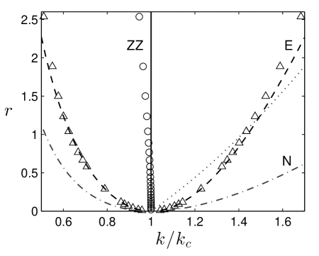
Figure 1: The stability diagram of the periodic solutions of Eq. (12) shows the neutral curve (N, dot-dashed line) according to Eq. (28), the Eckhaus stability boundary obtained for the one-mode solution via Eq. (49) (E, dashed line) and numerically (triangles), as well as the zig-zag stability boundary for the one-mode approximation given by Eq. (50) (ZZ, solid line) and as obtained numerically (circles). The wave number $\tilde{k}_{m}=\sqrt{1+r}$ at the maximum of the growth rate $\sigma$ is given by the dotted line.

In a full numerical analysis the nonlinear periodic solution is determined numerically, as described in more detail in Appendix A. Then the stability boundaries are determined by the conditions given in Eq. (44) and in Eq. (46), similar as for the one mode approximation above.

Alternatively, the stability of nonlinear periodic solutions is determined by a linear stability analysis, as described in Appendix A and in Appendix B analytically in the range $r\gtrsim 0$. The analysis of the functional and the linear stability analysis give identical stability boundaries.

The reduced control parameter range, $0<r<1$, corresponds to a moderately deep quench of the diblock copolymer melt and belongs to the so-called weak segregation regime. In this range the Eckhaus and zig-zag boundary, as obtained by the one-mode approximation in Eq. (40), coincide well with the numerical stability analysis, where several modes of the Fourier expansion in Eq. (39) are taken into account. In the range $r>1$ the spatial shape of the nonlinear periodic solutions becomes increasingly anharmonic and deviates from the one-mode solution given by Eq. (40). Accordingly, the results of the one-mode approximation, as given by Eq. (49) and Eq. (50), start to deviate from the full numerical results obtained for the Eckhaus boundary (triangles) and the zig-zag line (circles).

The dotted line in Fig. 1 shows the control parameter dependence of the wave number $\tilde{k}_{m}$ of the fastest growing perturbation with respect to the homogeneous state. The curve $\tilde{k}_{m}(r)$ crosses the Eckhaus boundary at $\tilde{k}=5^{1/4}\approx 1.5$, corresponding to $r=\sqrt{5}-1\approx 1.24$. Therefore, after a deep quench with $r>\sqrt{5}-1$, the wave number of lamellar structures developing during the early stages of microphase separation may lie in the unstable range to the right of the Eckhaus stability boundary. The processes required to relax the wave number of the periodic solution back to the stable wave number band leads to the appearance of many defects as discussed further in Sec. 5.

3.6 Strong segregation regime

With increasing of the control parameter $r$ (resp. $\varepsilon$) the spatially periodic solutions of Eq. (12) become rather anharmonic and for large values of $r$ they can be approximated by a square wave of the form

$$\psi(x)=a_{0}[1-2\Theta(x-\lambda/4)+2\Theta(x-3\lambda/4)],$$ (52)

with $0<x<\lambda$ and the Heaviside step function $\Theta(x)$. In this limit the Green’s function in Eq. (14) is given by $G(x,x^{\prime})=|x-x^{\prime}|/2$. The gradient square term in the free energy Eq. (14) can be calculated by using the hyperbolic tangent profile $\psi=\mp a_{0}\tanh[(x-x_{i})/\xi]$ with a small width $\xi$ of the interfaces at $x_{1}=\lambda/4$ and $x_{2}=3\lambda/4$ as an approximation of the step function. Within these approximations one obtains the following expression for the free energy per period $\lambda$:

$${\cal F}=-\frac{a_{0}^{2}}{2}\left(\varepsilon-\frac{a_{0}^{2}}{2}-\frac{16}{3\lambda\xi}-\frac{\alpha\lambda^{2}}{48}\right)\;.$$ (53)

A minimization of this expression with respect to $a_{0}$ gives

$$a_{0}^{2}=\varepsilon-\frac{16}{3\lambda\xi}-\frac{\alpha\lambda^{2}}{48}\;,$$ (54)

and with this amplitude the corresponding free energy can be further simplified to

$${\cal F}=-\frac{1}{4}a_{0}^{4}\;.$$ (55)

The equilibrium period of lamellae $\lambda_{e}$ corresponding to the minimum of the free energy is found by a minimization of Eq. (55) with respect to $\lambda$:

$$\lambda_{e}=4\left(\frac{2}{\alpha\xi}\right)^{1/3}\;.$$ (56)

In the strong segregation regime, i.e. $\varepsilon\gg\varepsilon_{c}$ (large $r$), or equivalently for $\alpha\to 0$ at a fixed $\varepsilon$, the width of the interface $\xi\to\sqrt{2/\varepsilon}$ becomes small ⁴⁸. In this case $\lambda_{e}$ at the minimum of ${\cal F}$ and the corresponding free energy per period ${\cal F}_{e}$ are given by

$$\lambda_{e} = 4(2\varepsilon)^{1/6}\alpha^{-1/3}\;,$$

$${\cal F}_{e} = -\frac{1}{4}\left[\varepsilon-(2\varepsilon\alpha)^{1/3}\right]^{2}\;.$$ (57)

The scaling $\lambda_{e}\sim\alpha^{-1/3}$ has to be compared with the scaling in the weak segregation limit $\lambda_{e}\sim\alpha^{-1/4}$ according to Eq. (51). The results for $\lambda_{e}$ and ${\cal F}_{e}$ obtained in weak and strong segregation regime, which are given by Eq. (51) and Eq. (3.6), respectively, are in each regime in good agreement with the results according to the full numerical solutions, as can be seen in Fig. 2.

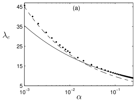
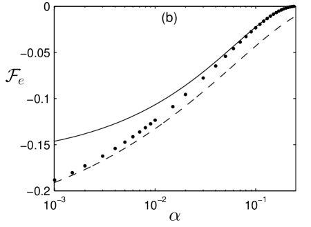
Figure 2: The lamella period $\lambda_{e}$ at the minimum of ${\cal F}(k)$ is shown in (a) as a function of $\alpha$ for $\varepsilon=1$ and in (b) the corresponding free energy ${\cal F}_{e}={\cal F}(\lambda_{e})$. The solid lines are obtained by Eq. (51) (weak segregation), the dashed lines by Eq. (3.6) (strong segregation). The bullets are the results of the full numerical calculations.

The transition from the weak segregation regime in the range $\alpha>0.02$ to the strong segregation regime in the range $\alpha<0.02$ is clearly visible in Fig. 2. The scaling exponents agree with those obtained earlier from variational calculations ³⁴ and numerical simulations ^{49, 50}.

4 Orientation of lamellae between substrates

The free energy of block copolymer films between two confining substrates depends on the orientation of lamellae with respect to the substrates, on the distance between the confining substrates and on the surface properties of the bounding substrates. In order to model for instance a BCP film with the lamellae perpendicular to a substrate, which is in addition laterally confined by parallel side walls as in Refs. ^{30, 31}, we consider in this section Eq. (12) in two spatial dimensions in the $x-y$ plane with boundaries at $y=0$ and $y=L_{y}$. This analysis applies as well to BCP confined between two extended plane parallel substrates.

The film thickness $L_{y}$ is given in terms of the dimensionless number $d$ and the wavelength $\lambda_{e}$:

$$L_{y}=d\ \lambda_{e}\;.$$ (58)

Boundary conditions. At plane substrates the boundary conditions for $\psi$ given by Eq. (18) and Eq. (21) take the following form,

$$\left.\frac{\partial}{\partial y}\left(-\varepsilon\psi+\psi^{3}-\nabla^{2}\psi\right)\right|_{y=0,\,L_{y}}=0\,,\qquad$$ (59a)

$$\qquad\,\left.\frac{\partial\psi}{\partial y}\right|_{y=0}=g(\psi-\psi_{0})|_{y=0}\;,$$ (59b)

$$\qquad\,\left.\frac{\partial\psi}{\partial y}\right|_{y=L_{y}}=g(\psi_{L_{y}}-\psi)|_{y=L_{y}}\;,$$ (59c)

with $\psi_{0}=\psi_{S}(y=0)$ and $\psi_{L_{y}}=\psi_{S}(y=L_{y})$.

Substrates preferentially wetted by one block of an $AB$ copolymer are described by finite values of $\psi_{0}$ and $\psi_{L_{y}}$, corresponding to so-called selective boundary conditions. We consider either symmetric selective boundary conditions at the two confining substrates, $\psi_{0}=\psi_{L_{y}}\not=0$, or antisymmetric ones, $\psi_{0}=-\psi_{L_{y}}\not=0$. Substrates being equally wetted by the $A$- and the $B$ block of a copolymer correspond to neutral boundary conditions, $\psi_{0}=\psi_{L_{y}}=0$. As a third example of confined copolymer films we investigate also mixed boundary conditions, when one substrate acts like a selective boundary and the opposite one like a neutral boundary.

With the wave vector ${\bf k}_{\perp}=(k,0)$ we describe the periodic order of lamellae perpendicular and with ${\bf k}_{\parallel}=(0,k)$ the periodic order of lamellae parallel to the substrates.

Numerical method: To find stationary solutions of Eq. (12) with the boundary conditions Eq. (59) a central difference approximation of the spatial derivatives is used. In the case of an orientation of lamellae parallel to the substrates one has to consider only the $y$ dependence of Eq. (12) and Newton’s iteration method is used for its solution. For lamellae perpendicularly oriented to the substrates two-dimensional simulations of Eq. (12) are required. In this case we use a simple relaxation method with the width of one period $L_{x}=\lambda_{e}$ along the $x$ direction.

For a given solution $\psi({\bf r})$ the total free energy $F=F_{b}+F_{s}$ is calculated by integrating Eq. (14) and Eq. (19) numerically. In order to determine the last term in Eq. (14), Poisson’s equation for the auxiliary function in Eq. (16) is solved numerically by a relaxation method. The spatial discretization was chosen to be $\delta x=\delta y=0.5$ for most of the calculations, which provide a relative error of the free energy less than $1$%. For a transition range, where the free energies of lamellae parallel and perpendicular to the substrates become comparable, the discretization was decreased to $\delta x=\delta y=0.25$ for the purpose of a precision higher than $0.2$%. Note, that the values for the total free energy $F$ presented in the following are divided by the system size $A=L_{x}\times L_{y}$, i.e. we use the free energy per unit system size.

4.1 Selective boundary conditions

In the case of homogeneous, selective boundary conditions with $\psi_{0},\psi_{L_{y}}\not=0$ at the substrates, lamellae parallel to the boundaries have a lower free energy than perpendicularly oriented ones, as shown in this section. If the values $\psi_{0},\psi_{L_{y}}$ have a magnitude similar to the maximum of the amplitude of $\psi(y)$ in the bulk, then the envelope of $\psi(y)$ is only slightly deformed near the boundaries.

In the case $\psi_{0}$ and $\psi_{L_{y}}$ agree with the extrema of $\psi(y)$ in the bulk, then also the boundary condition $\left.\partial_{y}\psi\right|_{y=0,L_{y}}\approx 0$ can be fulfilled at an extremum of a periodic function $\psi(y)$ without any deformation.

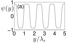
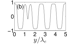
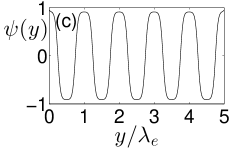
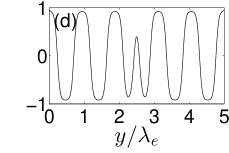
Figure 3: Four stationary solutions $\psi(y)$ of Eq. (12) in a film of thickness $L_{y}=5\lambda_{e}$ are shown for symmetric selective boundary conditions $\psi_{0}=\psi_{L_{y}}=1$. Part (a) and (c) show periodic solutions with an integer number of lamellae and part (b) and (d) so-called (unstable) saddle-point solutions. Parameters $\varepsilon=g=1$ and $\alpha=0.015$.

Examples of $\psi(y)$ for lamellae parallel to the boundary are shown in the case of selective boundary conditions, $\psi_{0}=\psi_{L_{y}}=1$, in Fig. 3(a) and Fig. 3(c) for a copolymer film of thickness $L_{y}=5\lambda_{e}$ in the strong segregation regime. The periodic field $\psi(y)$ in Fig. 3(a) and in Fig. 3(c) differs in the number of periods on the interval $[0,L_{y}]$, corresponding to different values of the wave number $k$. The wavelength of the solution with five periods in Fig. 3(c) corresponds to $\lambda=\lambda_{e}$ at the minimum of the free energy. In Fig. 3(a) the solution has four periods with a wavelength $\lambda>\lambda_{e}$ and this stationary solution in an unconfined system is unstable according to the results in Fig. 1. However, dynamical simulations show, that this wavelength is stabilized in a confined thin film. The solution in Fig. 4(e) has six periods on the interval $L_{y}=5\lambda_{e}$ and a wavelength $\lambda$ smaller than $\lambda_{e}$. This solution is according to the results presented in Fig. 1 expected to be stable in unconfined systems. The free energy $F/L_{y}$ of the solutions in Fig. 4(a) and (e) is larger than in Fig. 4(c) at the minimum of the free energy.

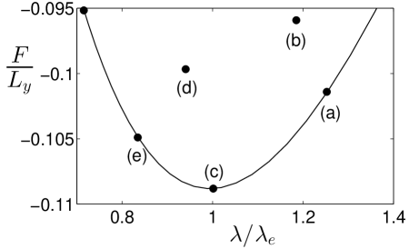
Figure 4: The normalized free energy $F/L_{y}$ of a copolymer film of thickness $L_{y}=5\lambda_{e}$ is shown as a function of the normalized width $\lambda/\lambda_{e}$ (solid line) for lamellae parallel to selective boundaries with $\psi_{0}=\psi_{L_{y}}=1$ and parameters as in Fig. 3. (a)-(d) mark the free energy of the corresponding solutions in Fig. 3.

The stationary solutions in Fig. 3(b) and Fig. 3(d) are so-called saddle point solutions, which are unstable. As the characteristic wavelength $\lambda$ of these two solutions we take the distance between two extrema in the ”undistorted” range of each solution. With this definition the solution in Fig. 3(d) has a wavelength between the wavelengths of the two solutions in Fig. 3(e) and (c) and the saddle point solution in Fig. 3(b) has a wavelength between that of the periodic solutions in Fig. 3(a) and (c). The free energy of both saddle point solutions is higher than that of the periodic solutions marked as (a), (c) and (e) in Fig. 4. The locally strong deformation of the periodic solutions in Fig. 3(b) and (d) may occur at different locations $y$ in the region $(0,L_{y})$, depending on the initial profile. In order to include or to remove one periodicity, as for instance by changing from the solution given in Fig. 3(a) to Fig. 3(c) or reversely, the local maximum of the saddle point solution Fig. 3(b) has to be crossed. Such energy barriers are essentially responsible that states with a wave number $k\neq k_{c}$ are stable in BCP films even if the wave number does not correspond to the minimum of the free energy.

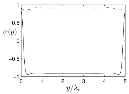
Figure 5: Stationary solutions of Eq. (12) for lamellae oriented perpendicularly to the boundaries at a position $x_{1}$ (dashed), where $\psi(x,y)$ takes its maximum in the bulk and at $x_{2}$ (solid), where $\psi(x,y)$ takes its minimum. The same parameters as in Fig. 3.

The $y$ dependence of the order parameter $\psi$ is rather different in the case of the lamellae perpendicular to selective boundaries. In this case $\psi(x,y)$ is a periodic function along the $x$ direction and selective boundary conditions force a finite value $\psi_{0,L_{y}}\not=0$ ($\psi_{0,L_{y}}>0$) at $y=0,L_{y}$, independent of the phase of the function. At positions $x_{1}$, where $\psi(x,y)$ takes its maximum in the bulk, the order parameter $\psi(x_{1},y)$ is nearly undeformed as a function of $y$, as can be seen by the dashed line in Fig. 5. However, the imposed selective boundary condition requires strong deformations of $\psi(x_{2},y)$ along the $y$ direction at positions $x_{2}$, where $\psi(x,y)$ takes its minimum in the bulk, as indicated by the solid line in Fig. 5. As a consequence of such strong deformations of $\psi(x_{2},y)$ near the boundaries, perpendicularly oriented lamellae have for selective boundary conditions a higher free energy than parallel oriented ones as shown in more detail in Fig. 6.

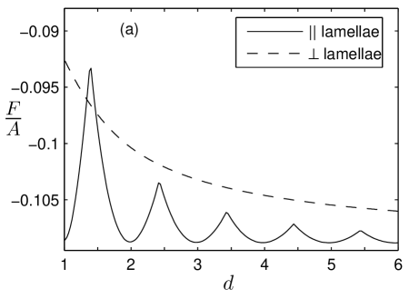
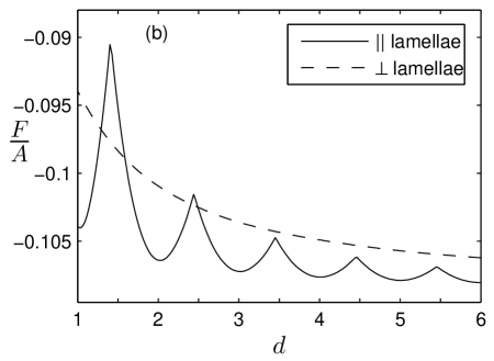
Figure 6: The free energy per unit area $F/A$ as a function of $d$ for lamellae parallel or perpendicular to symmetric selective boundaries in (a) with $\psi_{0}=\psi_{L_{y}}=1$ and in (b) with $\psi_{0}=\psi_{L_{y}}=0.5$. Parameters $\alpha=0.015$ and $\varepsilon=g=1$.

The free energy per unit area, $F_{\parallel}/A$, of a copolymer film with its lamellae parallel to the boundaries has as a function of the film thickness $L_{y}=d\lambda_{e}$ local minima at integer values of $d$ as indicated by the solid lines in Fig. 6(a) and Fig. 6(b). For parameters used in Fig. 6(a) the corresponding minima of the solid line have even an equal height. The dashed line in Fig. 6(a) shows the normalized free energy, $F_{\perp}/A$, of lamellae perpendicular to the substrate, which is for nearly all values of $d$ higher than $F_{\parallel}/A$. The periodically occurring strong variation of the order parameter $\psi(x_{2},y)$ for perpendicularly oriented lamella in the case of selective boundary conditions, as indicated at one position $x_{2}$ by the solid line in Fig. 5, enhances the free energy compared to the nearly undeformed function $\psi(y)$ in Fig. 3(a) for parallel lamellae.

The decay of $F_{\perp}(d)/A$ in Fig. 6(a) indicates that the weight of the strong deformation of $\psi(x,y)$ of perpendicularly oriented lamellae near the substrate becomes smaller with increasing thickness of the copolymer film. In Fig. 6(a) only for a very thin film-thickness of about $d\sim 1.5$ the free energy of parallel oriented lamellae is higher than for perpendicularly oriented ones.

In Fig. 6(b) the normalized free energies of parallel and perpendicularly oriented lamella are shown in the case of a reduced selectivity, $\psi_{0}=\psi_{L_{y}}=0.5$. Since the control parameter $\varepsilon$ (resp. $r$) is unchanged compared to the case in Fig. 6(a), a reduced value $\psi_{0}=\psi_{L_{y}}=0.5$ requires now a deformation of the function $\psi(y)$ at the boundaries also for parallel lamellae. This deformation increases the normalized free energy of parallel oriented lamellae, while the normalized free energy of perpendicularly oriented ones remains nearly unchanged, as can be seen by comparing the dashed lines in Fig. 6(a) and (b). This enhancement of the free energy is stronger for small values of $d$ than for larger values of $d$, because of the decreasing weight of boundary effects with increasing film thicknesses.

As a consequence of this energy enhancement in the case of a reduced preferential adsorption, there are now two maxima of the free energy of parallel lamellae in Fig. 6(b), at about $d\approx 1.5$ and $d\approx 2.5$, where the free energy is higher than that of lamellae perpendicular to the substrates. Such situations of confined diblock copolymers were also studied experimentally in thin films in the range $d=1.4-3.2$ by varying the selectivity of the substrates ¹². Here, a reduction of the preferential adsorption leads at about $d\approx 2.5$ to a frustration and lamellae perpendicularly oriented to the boundaries. However, in agreement with our simulations, for block copolymer films being less frustrated and also for strong preferential adsorption the parallel orientation of lamellae remains always preferred in this experiment.

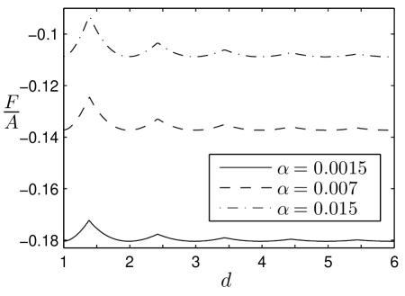
Figure 7: The free energy per unit area $F/A$ of lamellae parallel to the substrate as a function of $d$ for selective boundaries $\psi_{0}=\psi_{L_{y}}=1$ and different values of $\alpha$ and $\varepsilon=g=1$.

The normalized free energy of lamellae parallel to selective substrates becomes smaller with decreasing values of $\alpha$, as shown in Fig. 7. This trend is similar to the $\alpha$-dependence of the bulk free energy given by Eq. (51) [see Fig. 2(b)]. Since decreasing values of $\alpha$ correspond to increasing values of the thickness of the lamellae, the weight of surface effects decreases, that leads to a reduction of the peak height with $\alpha$, as can be seen in Fig. 7 too.

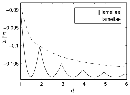
Figure 8: The free energy per unit area $F/A$ of parallel and perpendicularly oriented lamellae as a function of $d$ for asymmetric selective boundaries: $\psi_{0}=1,\psi_{L_{y}}=-1$. Parameters $\alpha=0.015$ and $\varepsilon=g=1$.

For asymmetric selective boundary conditions at the substrates, when one of the two substrates is preferentially wetted by one block and the other one by the second block of the copolymer, the normalized free energy of parallel lamellae has local minima at a film thickness close to a half-integer multiple of the equilibrium lamellar thickness $\lambda_{e}$, i.e. for $d=1.5,2.5,3.5,\dots$, as indicated by the solid line in Fig. 8. A situation with comparable free energies for lamella orientations parallel and perpendicular to asymmetric boundaries is only met in the range of very thin films of about $d\approx 2$. Otherwise the trend, that lamellae parallel to the substrates have for asymmetric selective boundaries a lower free energy, can be explained by the same arguments as given above for the case of symmetric selective boundary conditions.

By a reduction of the surface interaction strength $g$ (leading to non-interacting or quasi-periodic boundary conditions for $g\rightarrow 0$) or by a reduction of the preferred difference $\psi_{S}$ between the concentrations of $A$- and $B$ blocks at the boundary the free energies of both orientations can become comparable in the range of very thin films like in Fig. 6(b). However, in the range of thick films a parallel orientation of lamellae is always preferred in the case of selective boundary conditions. Detailed studies on that issue can be found elsewhere (see, e.g., ^{51, 52, 53, 54, 55}).

4.2 Neutral boundary conditions

Neutral boundaries with $\psi_{0}=\psi_{L_{y}}=0$ correspond to substrates, which are neither preferentially wetted by the $A$- nor by the $B$ block of a copolymer.

A first estimate of the expected preferred lamellae orientation may be gained by considering the effect of neutral boundaries in the weak segregation limit with small values of $r\gtrsim 0$. In this range a representation of $\psi=A\exp\left(i~{}{\bf k}_{\parallel,\perp}\cdot{\bf r}\right)+cc$ as in Eq. (32) is useful, where ${\bf k}_{\perp}=(k,0)$ is the wave vector in the $(x,y)$ plane of lamellae perpendicular and ${\bf k}_{\parallel}=(0,k)$ of lamellae parallel to the substrates. The envelope $A(x,y)$ decays in the case of neutral boundaries from its finite bulk value $A\propto\sqrt{r}$ to the boundary value $A\approx 0$. Such a reduction of the envelope causes an enhancement of the free energy per unit size compared to the case without boundary effects.

The transition layer, in which the envelope $A(x,y)$ changes from its bulk value to that at the boundary, is for perpendicularly oriented lamellae according to Eq. (38) proportional to $\xi_{2}\propto r^{-1/4}$, which is for small values of $r$ smaller than the transition layer of parallel oriented lamellae proportional to $\xi_{1}\propto r^{-1/2}$. Since the transition range is smaller in the case of lamellae perpendicular to the boundaries, we expect a smaller energy of perpendicularly oriented lamellae than for parallel oriented ones.

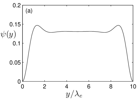
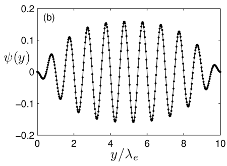
Figure 9: Stationary solutions of Eq. (12) for neutral boundary conditions $\psi_{0}=\psi_{L_{y}}=0$: In (a) at a position $x_{1}$ where $\psi(x,y)$ takes its maximum for lamellae perpendicular and in (b) parallel to the boundaries. In (b) the dots mark the analytical approximation as described in Appendix C for the same boundary condition. The parameters are $L_{y}=10\lambda_{e}$, $g=1$, $r=0.021$, $k=0.7$ (corresponding to $\varepsilon=1$ and $\alpha=0.24$).

Full numerical solutions of Eq. (12) by taking into account the boundary conditions (59) with $\psi_{0}=\psi_{L_{y}}=0$ are shown in Fig. 9 in the weak segregation limit at $r=0.021$ for perpendicularly oriented lamellae in part (a) and for parallel oriented lamellae in part (b). In Fig. 9(b) we show also the analytical approximation of the solution (symbols) for the same boundary conditions, as described in the Appendix C.

As indicated by the estimate in the previous paragraph, the length of the envelope of $\psi(y)$ needed for the transition from its value in the bulk to that at the boundary is indeed larger for parallel oriented lamellae than for the perpendicularly oriented ones. A narrower transition range causes a smaller enhancement of the free energy and therefore, in the range of small values of $r\gtrsim 0$ (weak segregation limit) lamellae perpendicularly oriented with respect to the substrates are energetically preferred. This behavior extends also to the strong segregation regime with larger values of $r$, as we have tested by further numerical calculations.

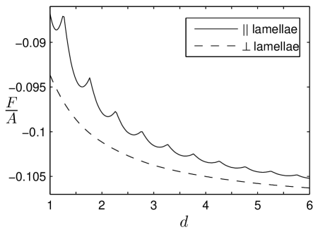
Figure 10: The free energy per unit area $F/A$ of parallel and perpendicularly oriented lamellae as a function of $d$ for neutral boundaries $\psi_{0}=\psi_{L_{y}}=0$ and the parameters $\alpha=0.015$, $\varepsilon=g=1$.

For numerical stationary solutions of Eq. (12) in the strong segregation regime the free energy of lamellae, that are perpendicularly oriented to neutral boundaries, does not differ very much from the free energy obtained in the case of selective boundaries, as can be seen by comparing the dashed curves in Fig. 6 and Fig. 10. On the other hand, the decay of the envelope of $\psi(x,y)$ close to the boundaries, as shown in Fig. 9(b), enhances the free energy of parallel lamellae compared to the case of selective boundaries, cf. Fig. 6. As a consequence of both trends, in the case of neutral boundaries perpendicularly oriented lamellae have always a lower free energy than parallel oriented ones, as shown in Fig. 10.

Note, that the free energy of parallel oriented lamellae has in the case of neutral boundaries local minima as a function of the film thickness close to integer and half-integer multiples of $\lambda_{e}$. The tendency of lamellae to align perpendicularly to the substrates in the case of neutral boundaries has been also found in Refs. ^{56, 51}

In the weak segregation limit, i.e. small values of $r$, approximate analytical solutions of Eq. (12) are derived for lamellae parallel to the substrates, as described in more detail in Appendix C. Depending on $\psi_{0}$ and $\psi_{L_{y}}$ such an analytical approximation can be very good as can be seen for example in Fig. 9(b).

4.3 Selective versus neutral boundaries

It depends on the ratio between the extremal values of the amplitude of $\psi$ in the bulk and the induced values at the boundaries whether the boundary conditions act more like selective or neutral boundary conditions. This can be recognized for instance by comparing the difference between the free energy of parallel and perpendicularly oriented lamellae in Fig. 6 and Fig. 10 for the three different values: $\psi_{0}=\psi_{L_{y}}=1$, $\psi_{0}=\psi_{L_{y}}=0.5$ and $\psi_{0}=\psi_{L_{y}}=0$. While in the case $\psi_{0}=\psi_{L_{y}}=1$ the maximum of $\psi(y)$ in the bulk is similar to the imposed value at the boundary, in the other two cases the maximum in the bulk is larger than at the boundaries.

The ratio between the maximum value and the value at the boundary can also be changed by changing the quench depth, i.e. by changing $r$ (respectively $\varepsilon$), but keeping now the values $\psi_{0}=\psi_{L_{y}}$ fixed. In this case the maximum bulk value can be either smaller or larger than the values at boundaries, depending on $r$. We found that for different values of $\psi_{0}=\psi_{L_{y}}$ variations of the control parameter $r$ do not induce a reorientation of the lamellae with respect to the boundaries.

4.4 Mixed boundary conditions

The results presented in the previous sections indicate that a combination of a selective and a neutral boundary condition may lead to almost equal energies for parallel and perpendicularly oriented lamellae over a large range of values of the film thickness $L_{y}$. Therefore, we compare in this section for mixed boundary conditions the free energies of homogeneously oriented lamellae parallel and perpendicular to the confining substrates.

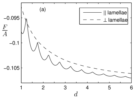
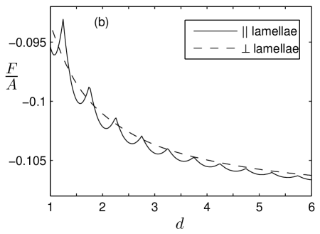
Figure 11: The free energy per unit area $F/A$ of parallel and perpendicularly oriented lamellae as a function of $d$ for mixed boundary conditions: In (a) $\psi_{0}=0$, $\psi_{L_{y}}=1$ and in (b) $\psi_{0}=0$, $\psi_{L_{y}}=0.5$. Parameters $\alpha=0.015$ and $\varepsilon=g=1$.

In Fig. 11 the free energy per unit size is shown as a function of $d$ for perpendicularly (dashed lines) and parallel (solid lines) oriented lamellae in the case of mixed boundaries with $\psi_{0}=0$ and either $\psi_{L_{y}}=1$ or $\psi_{L_{y}}=0.5$. One may compare these results with those given in Fig. 6 for symmetric selective boundary conditions $\psi_{0}=\psi_{L_{y}}=1,~{}0.5$. There are two major differences between the results in both figures. The energy differences between the two lamellae orientations are smaller for mixed boundary conditions in Fig. 11 and the free energy of parallel oriented lamellae now has local minima at integer and half integer values of $d$.

The trend indicated in Fig. 11 suggests that by changing the boundary condition at one surface from selective to neutral and keeping the other surface neutral, the preferred lamellae orientation can be changed from parallel to perpendicular.

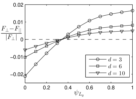
Figure 12: The relative free energy difference $(F_{\perp}-F_{\parallel})/|F_{\perp}|$ is shown for three thicknesses $L_{y}=3\lambda_{e},~{}6\lambda_{e},~{}10\lambda_{e}$ of the BCP film as a function of the selectivity $\psi_{L_{y}}$ at one boundary and $\psi_{0}=0$ at the opposite one. Beyond a critical value $\psi_{L_{y}}(crit)$ the preferred lamella orientation is parallel to the boundaries and perpendicular below. Parameters $\alpha=0.015$ and $\varepsilon=g=1$.

This is shown in Fig. 12, where the relative difference of the free energy $(F_{\perp}-F_{\parallel})/|F_{\perp}|$ is plotted as a function of $\psi_{L_{y}}$ for three different values of the film thickness $L_{y}=d\lambda_{e}$. Fig. 12 shows in addition that the critical value $\psi_{L_{y}}(crit)$, where both lamellae orientations have the same free energy, is rather independent of the film thickness $d$. This may be explained as follows. For the parameters used in Fig. 12 the two length scales introduced in Eq. (38) are nearly equal and both are small: $\xi_{1}/\lambda_{e}\approx 0.13$ and $\xi_{2}/\lambda_{e}\approx 0.1$. I.e. the influence of the boundary is similar for the three values of the film thickness in Fig. 12, only the weight of the influence is reduced by increasing the film thickness. The prior effect leads to a smaller slope of the curves with larger values of $d$ in Fig. 12.

The critical selectivity $\psi_{L_{y}}(crit)$ depends weakly on the parameter $\alpha$. For smaller values of $\alpha$ and therefore a larger lamella period $\lambda_{e}$, the critical value of $\psi_{L_{y}}(crit)$ is smaller. Thus lamellae with a larger period require a smaller selectivity of the surface to realign.

Note that in case of relatively thin films the free energy of parallel oriented lamellae as a function of thickness shows pronounced oscillations between local minima and maxima [see Fig. 11(a)]. This leads to a weak thickness dependence of the critical selectivity when considering the thicknesses that correspond to a maximum and a minimum of $F_{\parallel}$ (see Fig. 13). In the case of a maximum of $F_{\parallel}$ the reorientation takes place at higher values of $\psi_{L_{y}}$ than for a minimum. With increasing film thicknesses this difference is rapidly decreasing.

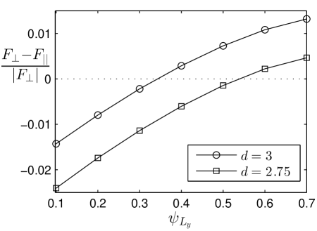
Figure 13: The relative free energy difference $(F_{\perp}-F_{\parallel})/|F_{\perp}|$ is shown as a function of the selectivity $\psi_{L_{y}}$ at one boundary with $\psi_{0}=0$ at the opposite one for two BCP films with $L_{y}=2.75\lambda_{e}$ (lower curve) and $L_{y}=3\lambda_{e}$ (upper curve). In both cases the preferred lamella orientation is parallel to the boundaries beyond a critical value $\psi_{L_{y}}(crit)$ and perpendicular below. Parameters $\alpha=0.015$ and $\varepsilon=g=1$.

5 Dynamics of microphase separation

The spatio-temporal dynamics of microphase separation in copolymers in two spatial dimensions between two parallel boundaries and the related lamellar (orientational) order is investigated here. We also describe typical differences between the evolution of structures in the strong and the weak segregation regime in BCP films confined between different boundaries on the one hand and in unconfined systems on the other hand.

For numerical simulations of Eq. (12) we use a central difference approximation of the spatial derivatives with $\delta x=\delta y=0.5$ and an Euler integration of the resulting ordinary differential equations with a time step $\Delta t=10^{-4}-10^{-3}$. In the unconfined case periodic boundary conditions are applied and a system size $L_{x}=L_{y}=256$ ($\approx 14\lambda_{e}$ for $\alpha=0.015$) is chosen. For block copolymer films of thickness $L_{y}=6\lambda_{e}$ between two substrates, different combinations of the boundary conditions along the $y$ direction are used, cf. Eqs. (59), and periodic boundary conditions along the $x$ direction with $L_{x}=4\lambda_{e}$, $8\lambda_{e}$, or $32\lambda_{e}$. To mimic a quench we start simulations of Eq. (12) with random initial conditions for $\psi$ of a small amplitude of about $10^{-4}$. Typical scenarios of the dynamics of microphase separation are studied in the strong segregation regime at a control parameter $\varepsilon=1$ ($r=3.08$) and in the weak segregation regime at $\varepsilon=0.37$ ($r=0.5$).

Microphase separation can be characterized by the structure factor of the evolving patterns,

$$S(\mathbf{k},t) = |\hat{\psi}(\mathbf{k},t)|^{2}\;,\;\;$$

$$\mbox{with}~{}\quad\hat{\psi}(\mathbf{k},t) = \int e^{i\mathbf{k}\cdot\mathbf{r}}\psi(\mathbf{r},t)d\mathbf{r}\;\,.$$ (60)

Since we expect anisotropy effects in BCP films confined between two substrates we introduce different characteristic lengths along the $x$ and the $y$ direction:

$$l_{x}(t)=\pi/\langle k_{x}\rangle(t)\;,\;\;l_{y}(t)=\pi/\langle k_{y}\rangle(t)\;.$$ (61)

The averaged wave numbers $\langle k_{i}\rangle$ are

$$\langle k_{x}\rangle(t)=\dfrac{{\int}_{0}^{k_{max}}dk_{x}{\int}_{-\Delta k}^{\Delta k}dk_{y}\,\,S(k_{x},k_{y},t)k_{x}}{{\int}_{0}^{k_{max}}dk_{x}{\int}_{-\Delta k}^{\Delta k}dk_{y}\,\,S(k_{x},k_{y},t)}\;,$$ (62a)

$$\langle k_{y}\rangle(t)=\dfrac{{\int}_{0}^{k_{max}}dk_{y}{\int}_{-\Delta k}^{\Delta k}dk_{x}\,\,S(k_{x},k_{y},t)k_{y}}{{\int}_{0}^{k_{max}}dk_{y}{\int}_{-\Delta k}^{\Delta k}dk_{x}\,\,S(k_{x},k_{y},t)}\;,$$ (62b)

where $\Delta k$ is the half-width of the corresponding peak of the structure factor along $k_{x}$ and $k_{y}$, respectively.

5.1 Unconfined systems

During microphase separation in diblock copolymers the most unstable perturbation with respect to the homogeneous basic state $\psi=0$ has the wave number $k_{m}=\sqrt{\varepsilon/2}$, cf. Eq. (27), similar as in binary mixtures ⁵⁷. The coarsening regime in diblock copolymers below $T_{c}$ is at early stages similar as in polymer blends, as indicated by two snapshots of a simulation in Fig. 14. In diblock copolymers the coarsening process of phase separation is limited by the chemical bond between an $A$- and $B$ block, which limits the domain size of phase separation to the order of the chain length of diblock copolymers.

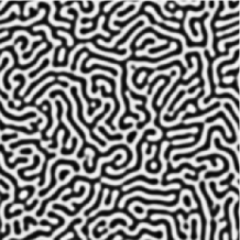
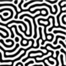
(a)                                 (b)

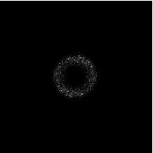
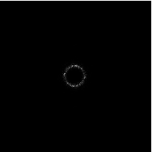
(c)                                 (d)

Figure 14: Microphase separation in the strong segregation regime for the parameters $\varepsilon=1$ ($r=3.08$) and $\alpha=0.015$ is shown in a two-dimensional system with $L_{x}=L_{y}=256\approx 14\lambda_{e}$ ($\lambda_{e}=19.3$) and periodic boundary conditions: In (a) at the time $t=10^{2}$ with the average wavelength of about $\lambda\approx 11.0$ and in (b) at $t=10^{4}$ with $\lambda\approx 17.5$. Dark and bright regions in the top part correspond to $A$- and $B$ block rich phases, respectively. The bottom part (c) and (d) show the corresponding structure factors, where the bright regions correspond to large values of $S(\mathbf{k},t)$.

The pattern shown in Fig. 14(b) has an average wavelength still below the optimal wavelength $\lambda_{e}$ at the minimum of the free energy. With a further progress of time the mean wavelength approaches only very slowly towards $\lambda_{e}$, because the system has to get rid of lamellar imperfections by diffusion processes.

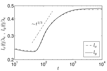
Figure 15: The temporal evolution of the characteristic length scales $l_{x}(t)$ and $l_{y}(t)$ (averaged over 10 independent runs) after a quench is shown in the strong segregation regime for the same parameters as in Fig. 14 and periodic boundary conditions.

Figure 16: The temporal evolution of the characteristic length scales $l_{x}(t)$ and $l_{y}(t)$ (averaged over 10 independent runs) after a quench is shown in the weak segregation regime at $\varepsilon=0.37$ ($r=0.5$) for a system with periodic boundary conditions and otherwise the same parameters as in Fig. 14 and in Fig. 15.

In an unconfined system the two length scales $l_{x}(t)$ and $l_{y}(t)$ evolve in a similar way and this isotropic behavior of the block copolymer melt is also reflected by the rotational symmetry of the structure factor shown by the parts (c) and (d) of Fig. 14. During the intermediate regime between the early stage of phase separation with a dominating growth of the perturbation of wave number $k_{m}$ and the late stage of coarsening with an average domain size, $l_{x}\approx l_{y}\approx\lambda_{e}/2$, one observes the scaling $l_{x}\sim l_{y}\sim t^{1/3}$ as shown in Fig. 15, which is common for polymer blends. Such a scenario is typical for a deep quench into the strong segregation regime at about $\varepsilon\sim 1$ and beyond.

In the weak segregation regime ($\varepsilon=0.37$ or smaller) the wave number of the fastest growing mode during the early stage of phase separation, $k_{m}=\sqrt{\varepsilon/2}$, is already closer to $2\pi/\lambda_{e}$ and therefore, one observes during pattern evolution only a slight variation of the scales $l_{x}(t)$ and $l_{y}(t)$, as shown in Fig. 16. Typical snapshots of phase separation during the early stage in the weak segregation regime are similar to patterns shown in Fig. 14(b).

5.2 Confined systems

For a block copolymer film confined between two selective boundaries with $\psi_{0}=\psi_{L_{y}}=1$, three snapshots during microphase separation in the strong segregation regime at $\varepsilon=1$ ($r=3.08$) are shown in Fig. 17, which will be compared later with results in the weak segregation limit.

After a deep quench at $t=0$ far below threshold $\varepsilon_{c}=2\sqrt{\alpha}$ (for $\alpha=0.0015$ one has $\varepsilon_{c}=0.077$) the selective boundary conditions trigger close to the substrates immediately a large value of the order parameter $\psi$ and in this case lamellae orient parallel to the substrates. One should note, that for the parameters in Fig. 17 the wavelength of the fastest growing mode $\lambda_{m}=2\pi/k_{m}=2\pi\sqrt{2/\varepsilon}=2\pi\sqrt{2}\approx 8.9$ is much smaller than the wavelength $\lambda_{e}=4(2\varepsilon)^{1/6}\alpha^{-1/3}\approx 39$ at the minimum of the free energy of a lamellar structure.

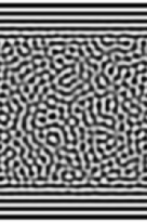
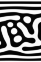
(a)                      (b)                      (c)

Figure 17: Microphase separation in a BCP film between two selective boundaries with $\psi_{0}=\psi_{L_{y}}=1$ is shown in the strong segregation regime at $\varepsilon=1$ ($r=3.08$) in (a) at time $t=20$ after the quench, in (b) at $t=40$, and in (c) at $t=10^{4}$ close to the final state. Parameters $L_{x}=4\lambda_{e}$, $L_{y}=6\lambda_{e}$, $\alpha=0.0015$ and $g=1$.

In the strong segregation regime the correlation lengths in the $x$ and $y$ direction are rather small and therefore a surface induced orientational order of the lamellae occurs only within short ranges near the boundaries as indicated by parts (a) and (b) in Fig. 17. Further away from the substrates the orientation of lamellae is only weakly influenced by boundary conditions and the lamellae are disordered, whereby this disorder resembles very much to that in the unconfined case, as shown in Fig. 14 and has also been observed in experiments on confined thin films ^{30, 31}. The average wavelength of the structure tends in the long time limit to $\lambda_{e}$.

Typical lamellar structures at the late stage of microphase separation in the strong segregation regime are shown in Fig. 18 for three types of boundary conditions. Neutral boundary conditions $\psi_{0}=\psi_{L_{y}}=0$ are used in Fig. 18(a), symmetric selective boundaries $\psi_{0}=\psi_{L_{y}}=1$ in Fig. 18(b) and in Fig. 18(c) mixed boundary conditions, $\psi_{0}=0$, $\psi_{L_{y}}=1$.

(a)

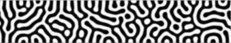
(b)

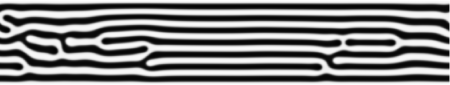
(c)

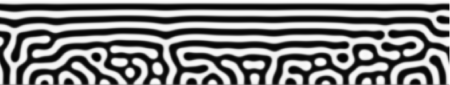
Figure 18: Microphase separation is shown in the strong segregation regime in a confined system at $t=10^{4}$ after a quench: In (a) for neutral, $\psi_{0}=\psi_{L_{y}}=0$, in (b) for symmetric selective, $\psi_{0}=\psi_{L_{y}}=1$, and in (c) for mixed boundary conditions, $\psi_{0}=0$, $\psi_{L_{y}}=1$. Parameters $L_{x}=32\lambda_{e}$, $L_{y}=6\lambda_{e}$, $\alpha=0.015$, $\varepsilon=1$ ($r=3.08$) and $g=1$.

The simulations of Eq. (12) were started with random initial conditions.

In the case of symmetric selective boundaries in Fig. 18(b) lamellae parallel to the substrates have the lower free energy as shown for the defect free lamellar order in Fig. 6. For neutral boundaries in Fig. 18(a) an orthogonal lamellae orientation close to a boundary is favored, which is in agreement with the results shown in Fig. 10. In the case of mixed boundary conditions in Fig. 18(c) lamellae are oriented parallel close to the selective (upper) boundary and perpendicular to the neutral (lower) boundary.

The pattern away from the boundaries in the bulk shows for neutral boundaries [Fig. 18(a)] a stronger disorder compared to the case of selective boundaries [Fig. 18(b)]. In the strong segregation regime the coherence lengths are small for both cases, but in the case of selective boundary conditions larger values of $\psi$ close to the boundary are induced and this causes a more regular lamellae orientation in the bulk.

The pattern Fig. 18(b) consists of seven periods parallel to the horizontal $x$-axis around the center of the image and six periods with $\lambda=\lambda_{e}$ close to the right end, whereby both regions are connected by a pattern including defects. The wave numbers corresponding to seven and six lamellae between the boundaries lie both in the range $k/k_{c}\geq 1$ of the stability diagram in Fig. 1, where a straight and defect free lamellar order is linearly stable with respect to small perturbations.

In simulations started with random initial conditions, patterns with $k_{m}>k_{c}$ grow with the largest rate and therefore a lamellar order with small wavelengths is preferred during the early stage of microphase separation. Since one has in Fig. 1 a wide wave number range $k>k_{c}$ of stable straight lamellae, a relaxation of a pattern like in Fig. 18(b) to the homogeneous state with six lamellae, which has the lowest free energy, is a long lasting process.

We showed in the previous section in Fig. 11(a) that in the case of mixed boundary conditions and parameters as in Fig. 18(c) a defect-free order of lamellae parallel to the substrates has a lower free energy than perpendicularly oriented ones. In simulations of extended systems with mixed boundaries, where patterns with defects may occur, neither a parallel nor a perpendicular orientation of lamellae is preferred in the bulk. Moreover, the pattern in Fig. 18(c) shows, that for mixed boundary conditions an orientational transition across the block-copolymer film can be expected, from parallel oriented lamellae at the selective (upper) boundary to a perpendicular lamellae orientation at the neutral (lower) boundary. The free energy of the pattern in Fig. 18(c) is higher than the free energy of parallel oriented lamellae as shown Fig. 11(a) and lower than that of perpendicularly oriented ones.

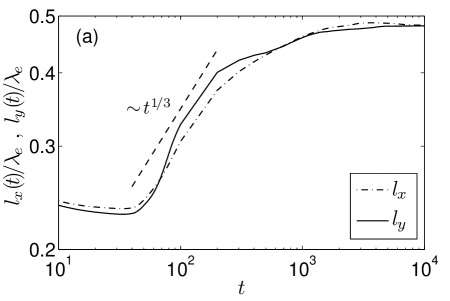
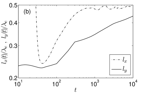
Figure 19: The time dependence of the characteristic length scales $l_{x}(t)$ and $l_{y}(t)$ (averaged over three runs) is shown in the strong segregation regime for the same parameters as in Fig. 18: (a) neutral boundaries, $\psi_{0}=\psi_{L_{y}}=0$, and (b) selective boundaries, $\psi_{0}=\psi_{L_{y}}=1$.

The temporal evolution of the lengths $l_{x}(t)$ and $l_{y}(t)$ in the case of neutral boundary conditions, as shown in Fig. 19(a), is rather similar to the unconfined case shown in Fig. 15. During the early stage of phase separation the dominating length scale is again that of the fastest growing mode, which is followed by the intermediate coarsening regime with $l_{x}\sim l_{y}\propto t^{1/3}$, before $l_{x}(t)$ and $l_{y}(t)$ terminate again at the typical length scale $\lambda_{e}/2$ of a diblock copolymer.

In the case of symmetric selective boundary conditions, $\psi_{0}=\psi_{L_{y}}=1$, the length scales $l_{x}$ and $l_{y}$ exhibit a different behavior during the initial stage of phase separation and especially the behavior of $l_{x}(t)$ is changed significantly, as shown in Fig. 19(b). A comparison of Fig. 17(a) and Fig. 17(b) reveals, that during the early stage of microphase separation compositional waves are induced by the selective boundaries and they propagate into the copolymer film. These induced composition waves near the boundaries have a quasi-infinite wavelength $l_{x}$ along the $x$ direction, while the wavelength $l_{y}$ along the $y$ direction behaves similar as in Fig. 19(a) for neutral boundaries. Far away from the selective boundaries one finds a random lamellae orientation and therefore $l_{x}$ behaves in the bulk at an intermediate and late stage of microphase separation similar as in the case of neutral boundaries.

(a)

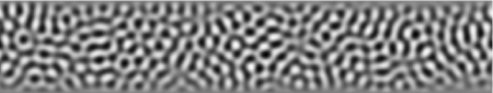
(b)

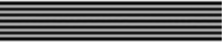
(c)

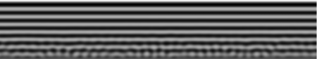
Figure 20: Microphase separation is shown in a confined system in the weak segregation regime with $\varepsilon=0.37$ ($r=0.5$) at the time $t=500$ after a quench and for three boundary conditions: (a) neutral, (b) symmetric selective and mixed in (c). Other parameters as in Fig. 18.

For comparison, we show in Fig. 20 late stage patterns in the weak segregation regime at $\varepsilon=0.37$ ($r=0.5$) for the same confined systems as in Fig. 18. These patterns show at a time $t=500$ already a similar order as in the strong segregation limit at $t=10^{4}$ (Fig. 18) in spite of the fact that the dynamics is slower for smaller values of the control parameter $r$. However, by a reduction of the control parameter from $r=3.08$ in the strong segregation limit to $r=0.5$ one has an enhancement of the length scales from $\xi_{1}\approx 0.13$ to $\xi_{1}\approx 0.32$ and from $\xi_{2}\approx 0.10$ to $\xi_{2}\approx 0.16$. These higher coherence lengths increase simultaneously the action range of the boundaries and both effects cause a higher lamellar order in a thin copolymer film within a shorter time (Fig. 20).

Similar as in the strong segregation regime one finds in the case of selective boundaries [Fig. 20(b)] again a higher lamellar order than in the case of neutral boundaries [Fig. 20(a)]. This is in agreement with the observation, that $\xi_{1}$ is for $r=0.5$ roughly by a factor of $2$ larger than $\xi_{2}$. This reasoning also confirms the results for the case of mixed boundaries [Fig. 20(c)], where the action range of the neutral (lower) boundary is smaller than that of the selective (upper) boundary.

The characteristic lengths $l_{x}(t)$ and $l_{y}(t)$ develop for $r=0.5$ and neutral boundaries again very similar as in the unconfined case in Fig. 16. In the case of selective boundaries [Fig. 20(b)] the two scales $l_{x}(t)$ and $l_{y}(t)$ show a similar behavior as in the strong segregation limit, only the saturation of $l_{y}(t)$ takes place already at $t\sim 10^{2}$.

In summary selective boundary conditions are more efficient for controlling the orientation of lamellae in copolymer films than neutral ones. A comparison of the results in Fig. 18 and in Fig. 20 suggests in addition that a quench to a small value of $\varepsilon\gtrsim\varepsilon_{c}$, followed by a further enhancement of $\varepsilon$ into the strong segregation regime, favors a coherent order of the lamellae. In the case of mixed boundary conditions one obtains ”mixed” lamellar structures as shown in Fig. 18(c), which can be also interpreted as a coexistence of two different boundary induced lamellae orientations.

As described in Sec. 4, different numbers of parallel oriented lamella between selective substrates can have at certain values of the distance $L_{y}$ between the boundaries equal free energies. For example at $L_{y}=4.4373$ and for parameters as given in Fig. 21 solutions with five and four lamellae parallel to the substrates have the same free energy. Such a coexistence is shown in Fig. 21 where the interface between both solutions does not move. This coexistence has a strong similarity for instance with observations presented in Fig. 3(a) in Ref.³⁰. This example indicates that in the case of a film thickness, which is not an integer multiple of $\lambda_{e}$, one may observe a spatial variation of the number of lamellae in a block copolymer film.

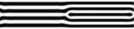
Figure 21: The spatial coexistence of structures with four and five lamellae parallel to the boundaries at a distance $L_{y}=4.4373\lambda_{e}$ is shown in the case of selective boundary conditions $\psi_{0}=\psi_{L_{y}}=1$. Parameters $\varepsilon=g=1$ and $\alpha=0.015$.

Also the free energy of parallel and perpendicularly oriented lamellae can be equal for certain boundary conditions and film thicknesses, as discussed in Sec. 4. In Fig. 22 we show an example for parameters, where parallel and perpendicularly oriented lamellae have the same free energy. According to the interface between both orientations the free energy of the structure in Fig. 22 is slightly higher than that of the pure parallel or perpendicular orientation. Nevertheless, as the interface between coexisting lamellae orientations in Fig. 22 is not moving the coexisting pattern is long lasting.

Figure 22: The spatial coexistence of structures with lamellae parallel and perpendicular to the boundaries at a distance $L_{y}=4.3854\lambda_{e}$ is shown in the case of selective boundary conditions $\psi_{0}=\psi_{L_{y}}=0.4$. Parameters $\varepsilon=g=1$ and $\alpha=0.015$.

5.3 Dynamics of orientational ordering

In diblock copolymers confined between boundaries the rotational symmetry is broken. The structure factor $S({\bf k},t)$ as well as the characteristic length scales $l_{x}$ and $l_{y}$, as introduced above, do not provide a sufficient quantitative characterization of the orientational order of lamellae. Besides the so-called Euler characteristics ⁵⁸ or a complex demodulation method ⁵⁹ the lamellar morphology may be described in the framework of a network analysis ^{60, 61}, as applied in this section.

A basic element of the following analysis is image processing and the open source library OpenCV ⁶² is used for the detection of the interfaces between the $A$- and $B$-rich regions in the 2-dimensional binarized images of the field $\psi(x,y)$. The curves along these interfaces are approximated by polygonal chains resulting into a set of segments of lengths $l_{i}$ with the corresponding segment orientation angle $\theta_{i}$ relative to the $x$-axis. These data allow the calculation of an average interface segment length

$$\langle l_{s}\rangle=\frac{1}{N}\sum_{i=1}^{N}l_{i}\;,$$ (63)

over which neighboring lamellae are parallel to each other, as well as the calculation of the average orientation of segments and the number of segments. These criteria offer an improved distinction between patterns of different morphology.

An order parameter of the segment distribution, similar to the order parameter in nematic liquid crystals ⁶³, is an appropriate quantity for a characterization of the lamellar patterns during microphase separation. Since the orientation angles $\theta_{i}$ and $\theta_{i}+\pi$ are equivalent, the order parameter is given by a symmetric second rank and traceless tensor

$$\hat{Q}=\begin{pmatrix}Q_{xx}&Q_{xy}\\ Q_{xy}&-Q_{xx}\end{pmatrix}\;,$$

$$Q_{xx}=\frac{\sum_{i=1}^{N}l_{i}\cos(2\theta_{i})}{\sum_{i=1}^{N}l_{i}}\;,$$

$$Q_{xy}=\frac{\sum_{i=1}^{N}l_{i}\sin(2\theta_{i})}{\sum_{i=1}^{N}l_{i}}\;.$$ (64)

With the scalar order parameter $S$ and the averaged orientation angle $\theta$ with respect to the $x$-axis,

$$S=\sqrt{Q_{xx}^{2}+Q_{xy}^{2}}\;,\;\;\theta=\frac{1}{2}\textrm{arccos}(Q_{xx}/S)\;.$$ (65)

With the unit vector (the director) $\mathbf{n}=(n_{x},n_{y})=(\cos\theta,\sin\theta)$ the tensor order parameter can also be written in the following form:

$$Q_{ij}=S(2n_{i}n_{j}-\delta_{ij})\;,$$ (66)

where $S$ has for perfectly ordered segments the value $S=1$ and for an isotropic orientational distribution of the segments one has $S=0$.

For the same parameters as used in Fig. 18 and Fig. 19 now the quantities $S$, $\theta$ and $\langle l_{s}\rangle$ are calculated as a function of time and the results are shown in Fig. 23. The snapshots in Fig. 18 indicate a significantly higher orientational order of the lamellae in the case of selective boundary conditions compared to neutral ones. This difference in the orientational order can now be quantified by comparing $S(t)$ for the two boundary conditions, as can be seen in Fig. 23(a).

The temporal evolution of the average boundary segment length $\langle l_{s}\rangle$ after a deep quench is shown in Fig. 23(c) and the mean orientation $\theta$ of segments in Fig. 23(b) for the three different boundary conditions: symmetric selective, neutral and mixed.

As can be already seen in Fig. 18, the average segment length of straight lamellae without defects takes in the thin film geometry its smallest value in the case of neutral boundary conditions. Simultaneously, one observes for neutral boundary conditions the smallest values of the scalar order parameter $S(t)$ on the time scale shown in Fig. 23(a) as well the strongest fluctuations of $\theta(t)$. Since the action length of the boundaries in the case of neutral boundary conditions is small and the removal of defects is a slow process, $\langle l_{s}\rangle$ increases only slowly as function of time ($\langle l_{s}\rangle\to L_{y}$ in the long time limit).

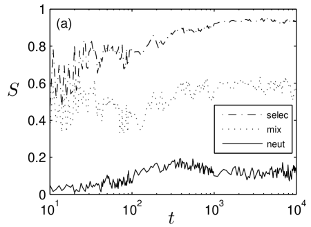
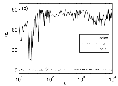
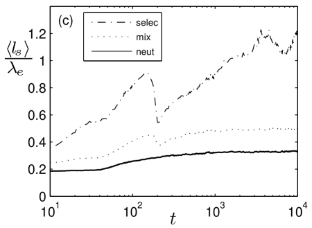
Figure 23: In part (a) the scalar order parameter $S$, in (b) the lamellae orientation angle $\theta$ [cf. Eq. (65)], and in (c) the averaged segment length $\langle l_{s}\rangle$ [cf. Eq. (63)] is shown in the strong segregation regime as a function of time for the same parameters as in Fig. 18 and Fig. 19 for the boundary conditions symmetric selective ($\psi_{0}=\psi_{L_{y}}=1$), symmetric neutral ($\psi_{0}=\psi_{L_{y}}=0$) and mixed ($\psi_{0}=0$, $\psi_{L_{y}}=1$).

(a)

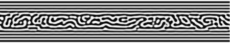
(b)

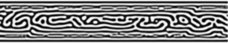
(c)

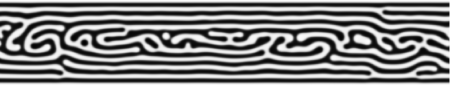
Figure 24: Snapshots of $\psi(x,y,t)$ at $t=100$ (a), $t=200$ (b) and $t=300$ (c) are shown for symmetric selective boundary conditions and the same parameters as in Fig. 18.

In the case of selective boundaries the action length of the substrates is larger and therefore oriented lamellae are formed much earlier. Consequently, one observes higher values of $\langle l_{s}\rangle$ and of the order parameter $S$ much earlier. The fact, that $S(t)$ has still not reached the value $S=1$ at about $t=10^{4}$ in Fig. 23(a) is related to the few defects left, as can be seen for instance in Fig. 18(b). As the regular structure is represented by lamellae parallel to the substrates, $\langle l_{s}\rangle\to L_{x}$ for long time dynamics. The reduction of $\langle l_{s}\rangle$ for selective boundaries at about $t=200$ in Fig. 23(c) is related to intermediate structures that occur during coarsening as indicated by the transition from the pattern in Fig. 24(a) to the pattern in Fig. 24(b).

The rather early achieved orientational order for selective boundaries is also indicated by the behavior of $\theta(t)$, which approaches zero quite early in Fig. 23(b). The large fluctuations of $\theta(t)$ in Fig. 23(b) for the neutral boundary conditions reflect the coarsening and the related removal of defects on the route to a higher orientational order. In this case the boundary segments are preferentially oriented perpendicular to the substrates resulting into the orientation angle $\theta\approx\pi/2$ for long-time evolution. In case of mixed boundaries, one obtains a mixing of both trends with respect to the orientation of lamellae. The selective (upper) surface triggers lamellae oriented parallel to the substrate whereas the neutral (lower) surface initiates lamellae oriented perpendicular to the substrate with less defects as for the two neutral boundaries [see Fig. 18(b)], and accordingly the results for $S$ and $\langle l_{s}\rangle$, represented by dotted lines in Fig. 23(a) and Fig. 23(c), lie between the two symmetric cases.

For comparison we show the temporal evolution of $S$, $\theta$ and $\langle l_{s}\rangle$ in Fig. 25 in the weak segregation regime with $\varepsilon=0.37$. Both, the behavior of $S(t)$ and of $\langle l_{s}\rangle$ confirm, that in the weak segregation regime an orientational order is reached on a smaller time scale as in the case of the strong segregation regime.

The composition waves with almost equilibrium wavelength result into $\langle l_{s}\rangle\approx L_{x}$ for the selective and mixed boundary conditions. The selective boundaries provide the fastest formation of regular parallel lamellae and therefore the fastest saturation of $\langle l_{s}\rangle$. In case of neutral boundaries $\langle l_{s}\rangle$ is increased faster in time compared to the deep quench [Fig. 23(c)] with the tendency $\langle l_{s}\rangle\to L_{y}$.

In case of a not too deep quench the scalar order parameter $S$ shown in Fig. 25(a) grows much faster in time compared to the deep quench. The boundary segments are again preferentially oriented perpendicular to the boundaries for the neutral boundary conditions and parallel to the boundaries for the selective and mixed boundary conditions [Fig. 25(b)].

Thus even this quite simple analysis of lamellar patterns provides quantitative characteristics of the dynamics and influence of the boundary conditions on the resulting patterns, that are complimentary to the standard analysis of the structure factor.

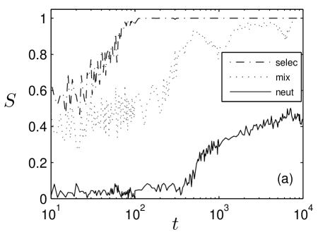
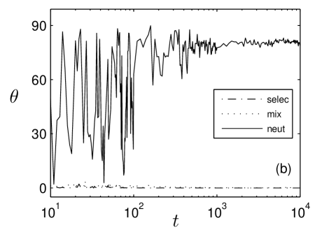
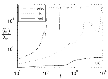
Figure 25: In part (a) the scalar order parameter $S$ and in (b) the lamellae orientation angle $\theta$ [cf. Eq. (65)], and in (c) the averaged segment length $\langle l_{s}\rangle$ [cf. Eq. (63)] is shown in the weak segregation regime as a function of time for the same parameters as in Fig. 20 for the boundary conditions, symmetric selective ($\psi_{0}=\psi_{L_{y}}=1$), symmetric neutral ($\psi_{0}=\psi_{L_{y}}=0$) and mixed ($\psi_{0}=0$, $\psi_{L_{y}}=1$).

6 Summary and conclusions

The formation and stability of lamellae in block copolymers has been investigated in terms of a mean-field model. A method for the determination of the stable wave number band has been introduced in Sec. 3 and the shape of this band provides the basis for a deeper understanding of stable lamellae conformations which are locked in experiments on BCP films to different wavelengths when using spatially periodic chemical nano patterning of substrates ²⁷.

We have found, similar as in previous calculations in terms of self-consistent mean field theories or phenomenological free energy models ^{53, 55}, that selective boundaries induce lamellae orientations parallel to the substrates and in the case of neutral boundaries lamellae orient perpendicular to surfaces. We present also estimates in terms of the different length scales parallel and perpendicular to the lamellae, whether lamellae orient parallel or perpendicular to confining boundaries. Some of the lamellae conformations calculated within this work resemble very much the lamellae orientations observed experimentally in thin BCP films at neutral substrates in Refs. ^{30, 31}. We derive also analytical expressions in the case of lamellae parallel to substrates for the concentration modulation perpendicular to the boundaries, which can be useful for qualitative considerations in further works.

In the case of mixed boundary conditions, i.e. selective at one boundary and neutral at the opposite boundary, we find a critical value ${\psi_{S}}(crit)$ of the selectivity below which the energetically preferred, homogeneous lamellae orientation changes from parallel to perpendicular with respect to the confining boundaries for any film thickness.

The results obtained are interesting also with regard to a recently used strategy to control the long range lamellae order in diblock copolymer films, where a thickness-dependent orientation of lamellae has been found ⁶⁴. While the lamellae oriented parallel to the substrate in the ranges of film thicknesses, $d<19$ and $d>23$, a perpendicular orientation in the range $19\leq d\leq 22$ was observed ⁶⁴. At a first sight, this experimental observation seems to be in contradiction to our results. However, these experiments were done in the presence of a solvent that changed the degree of swelling of the BCP film. Although our mean-field model does not contain explicitly the effects of a solvent on the lamellae formation and its interaction with surfaces, we suggest to use our results for an interpretation of the mentioned experiment. It has been found that in the presence of a solvent the degree of swelling $\phi=\lambda_{e}/\lambda_{s}$ (where $\lambda_{s}$ stands for the lamellae period in the swollen state) depends on the film thickness ⁶⁴. For very thin films ($d\approx 3$) the degree of swelling is around $\phi\approx 0.68$ whereas for thicker films ($d\approx 30$) it is about $\phi\approx 0.715$, which means, thicker films swell about $4\%$ less than thinner films and the concentration of the solvent $c_{s}$ is decreasing with increasing the film thickness. Accordingly, for thinner films in the swollen state we calculate an “effective value” of the model parameter $\alpha\sim\lambda^{-4}:$ $\alpha_{s}=(0.68)^{4}\alpha_{0}$ ($\alpha_{0}$ indicates the interaction parameter in the absence of a solvent). It is about $18\%$ smaller than for thick films where $\alpha_{s}=(0.715)^{4}\alpha_{0}$. Thus to model the influence of the solvent we can assume that the parameter $\alpha$ is effectively increased by increasing the film thickness. In addition our simulations reveal that the critical absorption at the surface, ${\psi_{S}}(crit)$, increases with $\alpha$. Assuming a linear behavior of ${\psi_{S}}(crit)$ as a function of $\alpha$

$${\psi_{S}}(crit)=a\cdot\alpha+b,$$ (67)

in a small range around $\alpha_{s}(d=30)/\alpha_{s}(d=3)\approx 1.2$, we calculate the slope $a\approx 14.8$. Therefore, in the range $d=3\cdots 30$,

$${\psi_{S}}(crit)[d=30]-{\psi_{S}}(crit)[d=3]\approx 0.7\alpha_{0}\;,$$ (68)

and ${\psi_{S}}(crit)$ increases slightly with the film thickness.

On the other hand the solvent may reduce the selectivity of the confining surface (see, e.g., ⁶⁵). Thus, ${\psi_{S}}$ is decreasing with an increasing solvent concentration. According to the swelling behavior it means that ${\psi_{S}}$ is increasing with increasing the film thickness $d$ as in thicker films the solvent concentration is lower. The exact form of the curve ${\psi_{S}}(d)$ can be determined experimentally by measuring the BCP-substrate interfacial tension in the swollen state for various film thicknesses.

Combining now the two effects, the addition of a solvent has, we end up with two curves that, depending on their relative position, offer the possibility for a reorientation effect of the lamellae as a function of the film thickness (see Fig. 26). The region where ${\psi_{S}}(d)<{\psi_{S}}(crit)$ indicates a possible transition region.

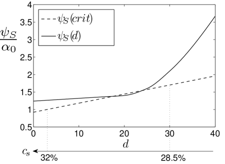
Figure 26: Critical value $\psi_{S}(crit)$ of the surface selectivity and $\psi_{S}$ rescaled by $\alpha_{0}$ as a function of $d$. The additional axis at the bottom indicates the solvent concentration $c_{s}$.

Of course the curve for ${\psi_{S}}(d)$ in Fig. 26 is to some extend hypothetical and the shape has to be determined experimentally via measuring the interfacial tension. Nevertheless, our results indicate a route for further experiments on the thickness-dependent lamellae reorientation. Especially for diblock copolymers with a pronounced change of the degree of swelling as a function of the film thickness (like, e.g., in ⁶⁶, where the increase of the solvent uptake with decreasing film thickness is more than $10$%) a considerably wide reorientation range may be realized by a suitable tuning of the wetting properties of the confining surfaces.

In addition to the energetic considerations of the influence of boundaries on the homogeneous lamellae orientations, we also investigated the dynamical evolution of lamellae structures between boundaries. In the case of mixed boundaries, one also finds complex lamellae conformations, even if they have a higher free energy than a homogenous lamellar order either parallel or perpendicular to the confining parallel boundaries. Simulations of the time-dependent mean field model show, that the type of boundary condition determines strongly the evolution of the orientational order as well as the number of defects in BCP films parallel and perpendicular to the boundaries, which has been quantified by using an order parameter for the characterization of the lamellae orientation. The consideration of different quench depths in combination with various boundary conditions provides a strategy for the experimental preparation of defect-free oriented lamellae.

We are grateful for inspiring discussions with W. Baumgarten, M. Hauser, M. Müller, W. Pesch and L. Tsarkova and for useful hints given by M. Khazimullin on using OpenCV. This work was supported by the German Science Foundation via the Research Center SFB 840 and the Research Unit FOR 608.

Appendix A Numerics of nonlinear solutions

Here we describe the numerical determination of stationary periodic solutions of Eq. (12) for $\beta=0$ as well as their linear stability. Since Eq. (12) is isotropic one can choose the $x$ direction parallel to the wave vector of the periodic solution. A Fourier expansion of the periodic solution $\psi_{k}(x)$, as given by Eq. (39), leads together with Eq. (12) after projection onto the $j$-th Fourier mode $e^{ikxj}$ to a set of nonlinear equations for the coefficients $A_{j}$:

$$[\varepsilon(jk)^{2}-(jk)^{4}-\alpha]A_{j}-(jk)^{2}\sum\limits_{l,m}A_{l}A_{m}A_{j-l-m}=0\;,$$

$$j=-M\ldots M\;.$$ (69)

For $M>1$ this system of nonlinear equations is solved numerically by Newton’s iteration method and $M$ is adjusted to keep the relative error smaller than $10^{-6}$. For $\varepsilon=1$ this accuracy can be maintained in the case of $\alpha=0.001$ with a very steep density profile by choosing $M=120$ modes and in the case of smoother density variations by $M=15$ modes. For larger values of $\alpha$ a smaller number of modes is required as the solution becomes more harmonic.

The linear stability of periodic solutions $\psi_{k}(x)$ of Eq. (12) with respect to small perturbations $\psi_{1}(x,y,t)$ is investigated as follows. One starts with the ansatz $\psi(x)=\psi_{k}(x)+\psi_{1}(x,y,t)$ and a linearization of the basic equation (12) with respect to $\psi_{1}(x,y,t)$ gives

$$\partial_{t}\psi_{1}(x,y,t)=\nabla^{2}\left(-\varepsilon+3\psi_{k}^{2}-\nabla^{2}\right)\psi_{1}-\alpha\psi_{1}\;,$$ (70)

wherein the spatially periodic function $\psi_{k}$ enters parametrically. For a solution of this linear equation (70) with periodic coefficients one uses a Floquet ansatz,

$$\psi_{1}(x,y,t)=e^{\sigma t}e^{is(x\cos\theta+y\sin\theta)}\phi_{F}(x)+\textrm{c.c.}\;,$$ (71)

with the Floquet parameter $s$, a $2\pi/k$-periodic function $\phi_{F}(x)$ and the angle $\theta$ enclosed between the wave vector of the perturbation $\psi_{1}$ and the wave vector of the basic periodic solution. This periodic function $\phi_{F}(x)$ can be represented by a Fourier expansion

$$\phi_{F}(x)=\sum_{n=-M}^{M}D_{n}~{}e^{ikxn}\;.$$ (72)

Taking into account Eq. (39) for $\psi_{k}$ the linear partial differential equation Eq. (70) is transformed after projection into an eigenvalue problem

$$\sigma D_{n}=\left\{\varepsilon C_{n}-C_{n}^{2}-\alpha\right\}D_{n}-3C_{n}\sum_{l,m}A_{l}A_{m}D_{n-l-m}\;,$$

$$C_{n}=(kn+s\cos\theta)^{2}+s^{2}\sin^{2}\theta\;,$$

$$n=-M\ldots M\;,$$ (73)

where the coefficients $A_{l}$ are determined by Eq. (A). We are interested in the growth rate $\sigma(\varepsilon,k,s,\theta)$, i.e., in the eigenvalue $\sigma$ with the largest real part. The condition $Re[\sigma(\varepsilon,k,s,\theta)]=0$ yields the stability boundaries $\varepsilon=\varepsilon_{0}(k,s,\theta)$. For $Re(\sigma)=0$ and $\theta=0$ one finds $\varepsilon=\varepsilon_{E}(k)$ that determines the Eckhaus boundary. In the case of $Re(\sigma)=0$ and $\theta=\pi/2$ the corresponding $\varepsilon=\varepsilon_{ZZ}(k)$ gives the zig-zag line.

Appendix B Stability of weakly nonlinear solutions

As described in Sec. 3.4 a periodic solution in a two-dimensional isotropic system may be destabilized by modulations along the wave vector (Eckhaus instability), undulations perpendicular to it (zig-zag instability), and a combination of both types (skewed varicose) ²⁸. Two of the instability branches are given in Fig. 1 and they may be determined analytically near threshold by analyzing the stability of the solution given by Eq. (35) for $P=0$ with respect to small perturbations $\delta A$:

$$A=A_{0}e^{iQx}+\delta A\;.$$ (74)

The analytical form of the perturbation is as follows:

$$\delta A=e^{\sigma t}e^{iQx}\{a_{1}\exp[is(x\cos\theta+y\sin\theta)]$$

$$\qquad\qquad+a_{2}\exp[-is(x\cos\theta+y\sin\theta)]\}\;.\qquad$$ (75)

A linearization of Eq. (33) with respect to small perturbations $\delta A$ leads for the growth rate $\sigma$ to a $2\times 2$ eigenvalue problem (see e.g. ^{28, 29}). In the special case $\theta=0$ and under the condition of neutral growth $\sigma=0$ the following expression for the control parameter $r_{E}$ at the Eckhaus stability boundary ($\theta=0$, longitudinal instability) follows:

$$r_{E}=\frac{6Q^{2}}{k_{c}^{2}}=6(\tilde{k}-1)^{2}\;.$$ (76)

A comparison with the neutral curve in Eq. (37) shows that the width of curve $r_{E}(Q)$ is narrower than $r_{N}(Q)$ by the famous factor

$$\frac{r_{E}(Q)}{r_{N}(Q)}=\frac{1}{\sqrt{3}}$$ (77)

for Eckhaus stability boundary ^{47, 46, 28, 29}.

The zig-zag stability boundary (transversal instability) results for the case $\theta=\pi/2$ and $\sigma=0$:

$$Q=0\;\textrm{, i.e.,}\;\;\tilde{k}_{ZZ}=1\;.$$ (78)

Hence, the stationary weakly nonlinear solution given by Eq. (35) is linearly stable in the region $Q\geq 0$ ($\tilde{k}\geq 1$) between the zig-zag line in Eq. (78) and the Eckhaus boundary $Q_{E}=\sqrt{rk_{c}^{2}/6~{}}$.

The results for the stability boundaries found so far in this appendix in the framework of the amplitude equation Eq. (33) are typically valid only in the vicinity of the critical point ($r\gtrsim 0$, $|k-k_{c}|\ll 1$). An essential improvement of the analytical results for the stability diagram can be obtained by the Galerkin approach in a one-mode approximation, as described in the following.

Inserting the ansatz given by Eq. (32) into Eq. (31) and projecting on the critical mode $e^{-ik_{c}x}$ one gets in the leading order

$$\partial_{t}A=\nabla^{2}_{k_{c}}[-2k_{c}^{2}(r+1)A+3|A|^{2}A-\nabla^{2}_{k_{c}}A]-k_{c}^{4}A\;,$$

$$\mbox{with}\qquad\nabla^{2}_{k_{c}}\equiv(\partial_{x}+ik_{c})^{2}+\partial_{y}^{2}\;.$$ (79)

Above threshold one may derive for the amplitude $A_{0}$ with the ansatz Eq. (35) via Eq. (B) the following expression:

$$A_{0}^{2}=\frac{2k_{c}^{2}}{3}\left[r-\frac{\big{[}(Q+k_{c})^{2}-k_{c}^{2}\big{]}^{2}}{2k_{c}^{2}(Q+k_{c})^{2}}\right]$$

$$\qquad=\frac{2k_{c}^{2}}{3}\left[r-\frac{(\tilde{k}^{2}-1)^{2}}{2\tilde{k}^{2}}\right]\;.$$ (80)

One can easily see that this amplitude $A_{0}$ vanishes at the neutral curve Eq. (28) for arbitrary values of $r$. Inserting perturbation Eq. (74) with the amplitude given by (B) into Eq. (B) the growth rate $\sigma$ is again calculated from a $2\times 2$ eigenvalue problem. The various stability boundaries are determined via the neutral stability condition $\sigma(r,Q,\theta)=0$ in terms of the control parameter $r(Q,\theta)$ by keeping simultaneously only the leading terms in $s$. Minimization of $r(Q,\theta)$ with respect to $\theta$ gives in the range $Q>0$ the angle $\theta=0$ and therefore an Eckhaus stability boundary

$$r_{E}=\frac{3\tilde{k}^{8}-2\tilde{k}^{6}-6\tilde{k}^{2}+5}{2\tilde{k}^{2}(\tilde{k}^{4}+3)}\;,$$ (81)

that coincides with the result obtained in the framework of the free energy considerations [see Eq. (49)]. For $\tilde{k}$ between the neutral curve given by Eq. (28) and the Eckhaus boundary in Eq. (81) the periodic solution in Eq. (35) with $A_{0}$ from Eq. (B) is unstable with respect to long-wavelength perturbations along the wave vector, i.e. $s\to 0$ and $\theta=0$.

In the vicinity of the band center $\tilde{k}=1$ one has in the leading order $r_{E}=6(\tilde{k}-1)^{2}+\cdots$ in agreement with the result derived via the standard amplitude equation [see Eq. (76)].

A minimization of $r(Q,\theta)$ in the range $Q<0$ gives the angle $\theta=\pi/2$ for the zig-zag instability line

$$Q_{ZZ}=0\;\textrm{, i.e.,}\;\;\tilde{k}_{ZZ}=1\;,$$ (82)

in agreement with Eq. (50). For the perturbations Eq. (74) with $s\to 0$, $\theta=\pi/2$ the growth rate $\sigma$ is negative for $\tilde{k}$ on the right hand side of the zig-zag line Eq. (82) up to the Eckhaus boundary Eq. (81).

A skew varicose instability with $0<\theta<\pi/2$ does not occur.

Appendix C Weakly nonlinear solution under confinement

Close to the onset of microphase separation ($r\gtrsim 0$) the dynamics of the amplitude of the periodic order parameter field $\psi(\mathbf{r})$ is governed by the Newell-Whitehead-Segel amplitude equation (33), as described in Sec. 3.2. This equation has spatially periodic solutions in extended systems as described in Sec. 3.2, but it may also be solved in the presence of boundaries.

Here we take into account boundary conditions for the case of lamellae oriented parallel to the substrates. With the ansatz

$$\psi(y)=\sqrt{\frac{2k_{c}^{2}r}{3}}~{}B(y)e^{ik_{c}(y-y_{0})}+\mbox{c.c.}\,.$$ (83)

one gets, starting from Eq. (31), the following equation of the envelope $B(y)$:

$$\frac{2}{rk_{c}^{2}}\partial_{y}^{2}B+\left(1-\mid B\mid^{2}\right)B=0\,.$$ (84)

This equation has constant solutions of the form

$$B_{0}(y)=B_{0}=\pm 1,$$ (85)

corresponding to a spatially periodic field $\psi(y)$ of constant amplitude.

Eq. (84) also has the solution

$$B(y)=B_{0}\tanh\left[\frac{k_{c}\sqrt{r}}{2}(y-\tilde{y})\right]\,$$ (86)

and this may be used to construct approximate solutions for lamellae parallel to the two boundaries. The decomposition (83) is based on the assumption, that $B(y)$ varies slowly on the scale $2\pi/k_{c}$ and close to threshold one may simplify the boundary conditions (59) to the following conditions,

$$\partial_{y}\psi|_{y=0,L_{y}}=0\,,$$ (87a)

$$\psi|_{y=0}=\psi_{0}=c\cdot\psi_{b}\,,$$ (87b)

$$\psi|_{y=L_{y}}=\psi_{L_{y}}=c\cdot\psi_{b}\,,$$ (87c)

by neglecting higher order derivatives of $\psi$. The constant $c$ is used to switch between different types of boundary conditions: $c=0$ corresponds to neutral boundaries, and $c\neq 0$ to selective (symmetric) boundaries.

In order to fulfill the boundary conditions (87) at $y=0$ and $y=L_{y}$, we use a linear superposition of the solution (86) of the form

$$B(y)=v_{1}+v_{2}Y_{1}(y)+v_{3}Y_{2}(y)\,,$$ (88)

where the constants $v_{1},v_{2},v_{3}$ indicate the possible signs $\pm 1$ and with

$$Y_{1}(y)=\tanh\left[\frac{k_{c}\sqrt{r}}{2}(y-y_{1})\right]\,,$$ (89a)

$$Y_{2}(y)=\tanh\left[\frac{k_{c}\sqrt{r}}{2}(y-y_{2})\right]\,.$$ (89b)

The constants $y_{1}$ and $y_{2}$ are determined by the boundary conditions.

With the bulk value

$$\psi_{b}=\sqrt{\frac{8k_{c}^{2}r}{3}}\,$$ (90)

the order parameter $\psi(y)$ takes the form

$$\psi(y)=\psi_{b}[v_{1}+v_{2}Y_{1}(y)+v_{3}Y_{2}(y)]\cos\left[k_{c}(y-y_{0})\right]\,.$$ (91)

Inserting Eq. (91) into the boundary conditions (87) one has the following equations

$$\left[v_{2}(1-Y_{1}^{2}(0))\frac{\sqrt{r}}{2}\right]\cos(k_{c}y_{0})+$$

$$[v_{1}+v_{2}Y_{1}(0)-v_{3}]\sin(k_{c}y_{0})=0\,,$$ (92a)

$$\left[v_{3}(1-Y_{2}^{2}(L_{y}))\frac{\sqrt{r}}{2}\right]\cos(k_{c}y_{0})+$$

$$[v_{1}+v_{2}+v_{3}Y_{2}(L_{y})]\sin(k_{c}y_{0})=0\,,$$ (92b)

$$[v_{1}+v_{2}Y_{1}(0)-v_{3}]\cos(k_{c}y_{0})=c\,,$$ (92c)

$$[v_{1}+v_{2}+v_{3}Y_{2}(L_{y})]\cos(k_{c}y_{0})=c\,$$ (92d)

for the determination of the constants of the ansatz. Here we assumed a system size $L_{y}=n\cdot(2\pi)/k_{c}$ and exploited the approximation that the boundaries do not influence each other so that $Y_{1}(L_{y})=1$ and $Y_{2}(0)=-1$. From this one may directly deduce $v_{1}=v_{3}=-v_{2}$.

In the following some special cases are considered to illustrate the high quality of this approximation. The cases of selective ($c=1$) or neutral ($c=0$) boundaries may be solved explicitly. For the case of neutral boundaries we obtain $k_{c}y_{0}=\pm\pi/2$, $y_{1}=0$ and $y_{2}=L_{y}$ as a solution [see Fig. 9 (b)]. $v_{1}$ remains arbitrary in this case. If $c=1$ the value at the boundary corresponds to the bulk value and this case is conform with the periodic one where $B(y)=\pm 1=\mbox{const.}$ and $y_{0}=0$ [see Fig. 27 (a)]. For $c<1$ the selectivity is reduced [see Fig. 27 (b)]. In this case an explicit solution is not possible but one may use the approximation $\sin(k_{c}y_{0})\approx 0$ if $c$ is not too small what corresponds to $y_{0}\approx 0$. With this approximation we find $Y_{1}(0)\approx c$ and $Y_{2}(L_{y})\approx-c$ and $v_{1}=-1$ as a solution. The example shown in Fig. 27 (b) is for $c=0.5$ what results in $y_{1}\approx-10.83$ and $y_{2}\approx L_{y}+10.83$. Although this is only an approximation it still fits very well the full numerical solution. Of course this case may be studied more accurately by taking into account the wave number change. In this case one has more free parameters to adjust reasonably. Furthermore in the case of mixed boundaries this approximation becomes more complex and higher order derivatives have to be taken into account. The solution of the resulting equations becomes involved and the advantage of the approximations gets lost in comparison with the full numerical solution of the problem.

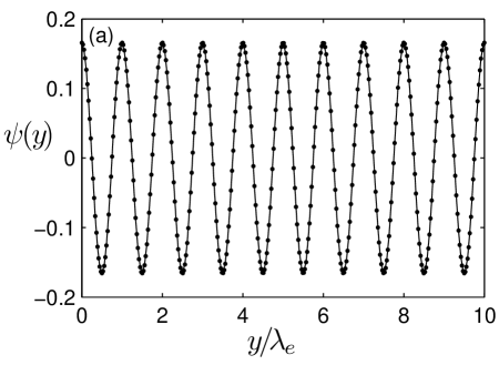
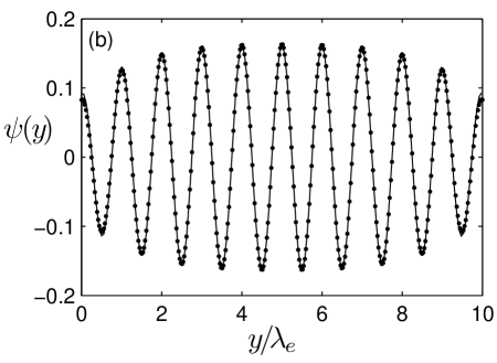
Figure 27: The numerical solution $\psi(y)$ of Eq. (12) is shown for various boundary conditions for lamellae parallel to the boundary: In part (a) for selective boundaries $c=1$ and in (b) for selective boundaries with a reduced selectivity $c=0.5$. The solid lines mark the numerical solution and the analytical approximation given by Eq. (91) is displayed by the dots. The parameters are $L_{y}=10\lambda_{e}$, $g=1$, $r=0.021$, $k_{c}=0.7$ (corresponding to $\varepsilon=1$ and $\alpha=0.24$).

References

- Bates et al. 1994 Bates, F. S.; Schulz, M. F.; Khandpur, A. K.; Förster, S.; Rosedale, J. H.; Almdal, K.; K., M. Faraday Discuss. 1994, 98, 7–18
- Förster et al. 1994 Förster, S.; Khandpur, A. K.; Zhao, J.; Bates, F. S.; Hamley, I. W.; Ryan, A. J.; Bras, W. Macromolecules 1994, 27, 6922–6935
- Matsen and Bates 1996 Matsen, M. W.; Bates, F. S. Macromolecules 1996, 29, 1091–1098
- Bates and Fredrickson 1999 Bates, F. S.; Fredrickson, G. H. Phys. Today 1999, 52, 32–38
- Fasolka and Mayes 2001 Fasolka, M.; Mayes, A. Annu. Rev. Mater. Res. 2001, 31, 323–355
- Segalman 2005 Segalman, R. A. Mater. Sci. Eng. R 2005, 48, 191–226
- Marencic and Register 2010 Marencic, A. P.; Register, R. A. Annu. Rev. Chem. Biomol. Eng. 2010, 1, 277–297
- Bang et al. 2009 Bang, J.; Jeong, U.; Ryu, D. Y.; Russell, T. P.; Hawker, C. J. Adv. Mater. 2009, 21, 4769–4792
- Hamley 2009 Hamley, I. Progress in Polymer Science 2009, 34, 1161–1210
- Gido et al. 1993 Gido, S. P.; Gunther, J.; Thomas, E. L.; Hoffman, D. Macromolecules 1993, 26, 4506–4520
- Fredrickson 1987 Fredrickson, G. H. Macromolecules 1987, 20, 2535–2542
- Kellogg et al. 1996 Kellogg, G.; Walton, D.; Mayes, A.; Lambooy, P.; Russell, T.; Gallagher, P.; Satija, S. Phys. Rev. Lett. 1996, 76, 2503–2506
- Amundson et al. 1991 Amundson, K.; Helfand, E.; Davis, D.; Quan, X.; Patel, S.; Smith, S. Macromolecules 1991, 24, 6546–6548
- Thurn-Albrecht et al. 2002 Thurn-Albrecht, T.; DeRouchey, J.; Russell, T.; Kolb, R. Macromolecules 2002, 35, 8106–8110
- Boker et al. 2002 Boker, A.; Knoll, A.; Elbs, H.; Abetz, V.; Muller, A.; Krausch, G. Macromolecules 2002, 35, 1319–1325
- Xu et al. 2007 Xu, T.; Wang, J.; Russell, T. P. In Nanostructured Soft Matter: Experiment, Theory, Simulation and Perspective; Zvelindovsky, A. V., Ed.; Springer: Dordrecht, 2007; pp 171–198
- Albalak and Thomas 1993 Albalak, R.; Thomas, E. J. Polym. Sci., Part B: Polym. Phys. 1993, 31, 37–46
- Wiesner 1997 Wiesner, U. Macromol. Chem. Phys. 1997, 198, 3319–3352
- Angelescu et al. 2004 Angelescu, D.; Waller, J.; Adamson, D.; Deshpande, P.; Chou, S.; Register, R.; Chaikin, P. Adv. Mater. 2004, 16, 1736–1739
- Hashimoto et al. 1999 Hashimoto, T.; Bodycomb, J.; Funaki, Y.; Kimishima, K. Macromolecules 1999, 32, 952–954
- De Rosa et al. 2000 De Rosa, C.; Park, C.; Thomas, E.; Lotz, B. Nature 2000, 405, 433–437
- Yoon et al. 2006 Yoon, J.; Lee, W.; Thomas, E. L. Adv. Mater. 2006, 18, 2691–2695
- Berry et al. 2007 Berry, B. C.; Bosse, A. W.; Douglas, J. F.; Jones, R. L.; Karim, A. Nano Lett. 2007, 7, 2789–2794
- Segalman et al. 2001 Segalman, R.; Yokoyama, H.; Kramer, E. Adv. Mater. 2001, 13, 1152–1155
- Cheng et al. 2006 Cheng, J. Y.; Ross, C. A.; Smith, H. I.; Thomas, E. L. Adv. Mater. 2006, 18, 2505–2521
- Bita et al. 2008 Bita, I.; Yang, K. W.; Jung, Y. S.; Ross, C. A.; Thomas, E. L.; Berggren, K. K. Science 2008, 321, 939–943
- Kim et al. 2003 Kim, S.; Solak, H.; Stoykovich, M.; Ferrier, N.; de Pablo, J.; Nealey, P. Nature 2003, 424, 411–414
- Cross and Hohenberg 1993 Cross, M. C.; Hohenberg, P. C. Rev. Mod. Phys. 1993, 65, 851–1112
- Cross and Greenside 2009 Cross, M.; Greenside, H. Pattern Formation and Dynamics in Nonequilibrium Systems; Cambridge University Press: New York, 2009
- Park et al. 2007 Park, S.-M.; Stoykovich, M. P.; Ruiz, R.; Zhang, Y.; Black, C. T.; Nealey, P. F. Adv. Mater. 2007, 19, 607–611
- Han et al. 2010 Han, E.; Kang, H.; Liu, C. C.; Nealey, P. F.; Copalan, P. Adv. Mater. 2010, 22, 43254329
- Gunton et al. 1983 Gunton, J. D.; San Miguel, M.; Sahni, P. In Phase Transitions and Critical Phenomena; Domb, C., Lebowitz, J. L., Eds.; Academic Press: London, 1983; Vol. 8; pp 267–466
- Leibler 1980 Leibler, L. Macromolecules 1980, 13, 1602–1617
- Ohta and Kawasaki 1986 Ohta, T.; Kawasaki, K. Macromolecules 1986, 19, 2621–2632
- Hashimoto et al. 1983 Hashimoto, T.; Shibayama, M.; Kawai, H. Macromolecules 1983, 16, 1093–1101
- Choksi and Ren 2003 Choksi, R.; Ren, X. J. Stat. Phys. 2003, 113, 151–176
- Bates and Hartney 1985 Bates, F. S.; Hartney, M. A. Macromolecules 1985, 18, 2478–2486
- Sakamoto and Hashimoto 1995 Sakamoto, N.; Hashimoto, T. Macromolecules 1995, 28, 6825–6834
- Cahn and Hilliard 1958 Cahn, J. W.; Hilliard, J. E. J. Chem. Phys. 1958, 28, 258–267
- Chen and Chakrabarti 1998 Chen, H.; Chakrabarti, A. J. Chem. Phys. 1998, 108, 6897–6905
- Binder 1983 Binder, K. In Phase Transitions and Critical Phenomena; Domb, C., Lebowitz, J. L., Eds.; Academic: New York, 1983; Vol. 8; pp 1–144
- Newell and Whitehead 1969 Newell, A. C.; Whitehead, J. A. J. Fluid Mech. 1969, 38, 279–303
- Newell et al. 1993 Newell, A. C.; Passot, T.; Lega, J. Annu. Rev. Fluid Mech. 1993, 25, 399–453
- Shiwa 1997 Shiwa, Y. Phys. Lett. A 1997, 228, 279–282
- Kramer and Hohenberg 1984 Kramer, L.; Hohenberg, P. Physica D 1984, 13, 357–369
- Kramer and Zimmermann 1985 Kramer, L.; Zimmermann, W. Physica D 1985, 16, 221–232
- Eckhaus 1965 Eckhaus, W. Studies in Nonlinear Stability Theory; Springer: New York, 1965; p 93 ff.
- Weith et al. 2009 Weith, V.; Krekhov, A.; Zimmermann, W. Eur. Phys. J. B 2009, 67, 419–427
- Oono and Bahiana 1988 Oono, Y.; Bahiana, M. Phys. Rev. Lett. 1988, 61, 1109–1111
- Liu and Goldenfeld 1989 Liu, F.; Goldenfeld, N. Phys. Rev. A 1989, 39, 4805–4810
- Geisinger et al. 1999 Geisinger, T.; Muller, M.; Binder, K. J. Chem. Phys. 1999, 111, 5241–5250
- Wang et al. 2000 Wang, Q.; Yan, Q.; Nealey, P.; de Pablo, J. J. Chem. Phys. 2000, 112, 450–464
- Matsen 1997 Matsen, M. J. Chem. Phys. 1997, 106, 7781–7791
- Pickett et al. 1993 Pickett, G.; Witten, T.; Nagel, S. Macromolecules 1993, 26, 3194–3199
- Walton et al. 1994 Walton, D.; Kellogg, G.; Mayes, A.; Lambooy, P.; Russell, T. Macromolecules 1994, 27, 6225–6228
- Lee et al. 1999 Lee, B.; Douglas, J.; Glotzer, S. Phys. Rev. E 1999, 60, 5812–5822
- Langer 1971 Langer, J. S. Ann. Phys. (N.Y.) 1971, 65, 53–86
- Mecke 1996 Mecke, K. R. Phys. Rev. E 1996, 53, 4794–4800
- Marietti et al. 2001 Marietti, Y.; Debierre, J.-M.; Bock, T. M.; Kassner, K. Phys. Rev. E 2001, 63, 066302
- Campbell et al. 2012 Campbell, I. P.; Lau, G. J.; Feaver, J. L.; Stoykovich, M. P. Macromolecules 2012, 45, 1587–1594
- Pujari et al. 2012 Pujari, S.; Keaton, M. A.; Chaikin, P. M.; Register, R. A. Soft Matter 2012, 8, 5358–5363
- Bradski 2000 Bradski, G. Dr. Dobb’s Journal of Software Tools 2000,
- de Gennes and Prost 1993 de Gennes, P. G.; Prost, J. The Physics of Liquid Crystals; Clarendon Press: Oxford: Oxford, 1993
- Olszowka et al. 2009 Olszowka, V.; Tsarkova, L.; Boeker, A. Soft Matter 2009, 5, 812–819
- Cavicchi et al. 2005 Cavicchi, K.; Berthiaume, K.; Russell, T. Polymer 2005, 46, 11635–11639
- Zettl et al. 2010 Zettl, U.; Knoll, A.; Tsarkova, L. Langmuir 2010, 26, 6610–6617