Abstract:

We present a determination of a set of polarized parton distributions (PDFs) of the nucleon, at next-to-leading order, from a global set of longitudinally polarized deep-inelastic scattering data: NNPDFpol1.0. The determination is based on the NNPDF methodology: a Monte Carlo approach, with neural networks used as unbiased interpolants, previously applied to the determination of unpolarized parton distributions, and designed to provide a faithful and statistically sound representation of PDF uncertainties. We present our dataset, its statistical features, and its Monte Carlo representation. We summarize the technique used to solve the polarized evolution equations and its benchmarking, and the method used to compute physical observables. We review the NNPDF methodology for parametrization and fitting of neural networks, the algorithm used to determine the optimal fit, and its adaptation to the polarized case. We finally present our set of polarized parton distributions. We discuss its statistical properties, test for its stability upon various modifications of the fitting procedure, and compare it to other recent polarized parton sets, and in particular obtain predictions for polarized first moments of PDFs based on it. We find that the uncertainties on the gluon, and to a lesser extent the strange PDF, were substantially underestimated in previous determinations.

1 Introduction

The interest in the determination of polarized parton distributions (PDFs) of the nucleon is largely related to the experimental discovery in the late 80s that the singlet axial charge of the proton is anomalously small [1, 2], soon followed by the theoretical realization [3, 4] that the perturbative behavior of polarized PDFs deviates from parton model expectations, according to which gluons decouple in the asymptotic limit. The theoretical interpretation of these results has spawned a huge literature, while at the same time experimental information on polarized PDFs from deep-inelastic scattering but also from a variety of other processes has been accumulating over the years (see e.g. [5] and references therein).

First studies of the polarized structure of the nucleon were aimed at an accurate determination of polarized first moments (including detailed uncertainty estimates) [6, 7, 8], but did not attempt a determination of a full PDF set, which was first proposed in Ref. [9], but without uncertainty estimation. More recently, polarized PDF sets with uncertainties have been constructed by at least four groups (BB [10, 11], AAC [12], LSS [13, 14] and DSSV [68, 15]). These PDF sets slightly differ in the choice of datasets, the form of PDF parametrization, and in several details of the QCD analysis (such as the treatment of higher twist corrections), but they are all based on the standard Hessian methodology for PDF fitting and uncertainty determination, which has been widely used in the unpolarized case (see [16, 17] and references therein). This methodology is known [16] to run into difficulties especially when information is scarce, because of the intrinsic bias of the Hessian method based on a fixed parton parametrization. This is likely to be particularly the case for polarized PDFs, which rely on data both less abundant and less accurate than their unpolarized counterparts.

In order to overcome these difficulties, the NNPDF collaboration has proposed and developed a new methodology for PDF determination [18, 19, 20, 21, 22, 23, 24, 25, 26, 27, 28, 29]. The NNPDF technique uses a robust set of statistical tools, which include Monte Carlo methods for error propagation, neural networks for PDF parametrization, and genetic algorithms for their training. The NNPDF sets are now routinely used by the Tevatron and LHC collaborations in their data analysis and for data-theory comparisons. In this work we extend the application of the NNPDF methodology to the determination of polarized parton distributions of the nucleon. As we will see, some PDF uncertainties will turn out to be underestimated in existing PDF determinations: in particular those of the polarized gluon distribution, but also those of the strange distribution.

The outline of this paper is as follows. In Sect. 2 we present the data set used to determine polarized PDFs, and we review the relationship between measured asymmetries and structure functions. In Sect. 3 we discuss the parametrization of polarized PDFs in terms of neural networks, and the construction of polarized structure functions. Then in Sect. 4 we discuss the minimization strategy. The results for the NNPDFpol1.0 polarized partons are presented in Sect. 5, and in Sect. 6 we discuss the phenomenological implications for the spin content of the proton and the test of the Bjorken sum rule. Finally in Sect. 7 we summarize our results and outline future developments. Some details on the benchmarking of polarized PDF evolution are given in the Appendix.

2 Experimental data

The bulk of the experimental information on (longitudinal) polarized proton structure comes from inclusive polarized deep-inelastic scattering with charged lepton beams. Deep-inelastic scattering with longitudinally polarized beams and targets allows a determination of the longitudinal structure function $g_{1}(x,Q^{2})$, which in turn admits a factorized expression in terms of polarized PDFs. Neutral-current deep-inelastic scattering does not allow to us to disentangle the contribution of quarks and antiquarks. Using both proton and neutron (deuteron or ³He) targets it is possible to separate the isospin singlet and triplet quark contributions to structure functions, with the gluon determined from scaling violations. A weak control on the separation of the isospin singlet quark contribution into its SU(3) octet and singlet component is possible using baryon decays to fix the respective normalization of these contributions, with in principle their different scale dependence providing some constraint on their shape.

Only charged-current deep-inelastic scattering would allow for full flavor separation [30]: this could be feasible with neutrino beams (such as available at a neutrino factory [31]), or perhaps very high-energy polarized charged lepton beams (such as available at an electron-ion collider [32]). Therefore, current constraints on flavor separation are only provided by semi-inclusive deep-inelastic scattering data or by polarized hadron collider processes, such as polarized Drell-Yan production in fixed target collisions and polarized $W$ production at the relativistic Heavy Ion Collider (RHIC). Likewise, direct constraints on the medium and large-$x$ polarized gluon require hadron and jet production either in fixed target experiments or at RHIC, while the small-$x$ gluon can only be probed by going to higher energy, such as at a polarized Electron-Ion Collider.

In this paper we will concentrate on inclusive longitudinally polarized DIS data, and thus we will only determine a subset of PDF combinations. This first polarized PDF set based on NNPDF methodology will then be available for inclusion of other datasets through the reweighting technique of Refs. [24, 28].

We will first review the experimental observables which we use for the determination of polarized structure functions, and the information which various experiments provide on them. Then, we will summarize the features of the data we use, and finally the construction and validation of the Monte Carlo pseudodata sample from the input experimental data.

2.1 Experimental observables and longitudinal polarized structure functions

Standard perturbative factorization provides predictions for polarized structure functions $g_{1}(x,Q^{2})$. However, experiments measure cross section asymmetries, defined by considering longitudinally polarized leptons scattering off a hadronic target, polarized either longitudinally or transversely with respect to the collision axis, from which the longitudinal ($A_{\parallel}$) and transverse ($A_{\perp}$) asymmetries are determined as

$$A_{\parallel}=\frac{d\sigma^{\rightarrow\Rightarrow}-d\sigma^{\rightarrow\Leftarrow}}{d\sigma^{\rightarrow\Rightarrow}+d\sigma^{\rightarrow\Leftarrow}};\quad A_{\perp}=\frac{d\sigma^{\rightarrow\Uparrow}-d\sigma^{\rightarrow\Downarrow}}{d\sigma^{\rightarrow\Uparrow}+d\sigma^{\rightarrow\Downarrow}}.\quad$$ (1)

The hadronic tensor for polarized, parity conserving deep-inelastic scattering can be parametrized in terms of four structure functions: two of them, $F_{1}(x,Q^{2})$ and $F_{2}(x,Q^{2})$, characterize spin-averaged deep-inelastic scattering, while $g_{1}(x,Q^{2})$ and $g_{2}(x,Q^{2})$ appear when both the lepton beam and the nucleon target are in definite polarization states. For the conventional definition of the hadronic tensor in terms of structure functions, see e.g. [33].

The two polarized structure functions are related to the measurable asymmetries Eq. (1) by

$$g_{1}(x,Q^{2}) =\frac{F_{1}(x,Q^{2})}{(1+\gamma^{2})(1+\eta\zeta)}\left[(1+\gamma\zeta)\frac{A_{\parallel}}{D}-(\eta-\gamma)\frac{A_{\perp}}{d}\right]\mbox{ ,}$$ (2)

$$g_{2}(x,Q^{2}) =\frac{F_{1}(x,Q^{2})}{(1+\gamma^{2})(1+\eta\zeta)}\left[\left(\frac{\zeta}{\gamma}-1\right)\frac{A_{\parallel}}{D}+\left(\eta+\frac{1}{\gamma}\right)\frac{A_{\perp}}{d}\right]\mbox{ .}$$ (3)

In Eqs. (2-3) the dependence on the nucleon mass $m$ is taken into account through the factor

$$\gamma^{2}\equiv\frac{4m^{2}x^{2}}{Q^{2}},$$ (4)

which also appears in the definitions of the other kinematic factors in Eqs. (2-3):

$$d =\frac{D\sqrt{1-y-\gamma^{2}y^{2}/4}}{1-y/2},$$ (5)

$$D =\frac{1-(1-y)\epsilon}{1+\epsilon R(x,Q^{2})},$$ (6)

$$\eta =\frac{\epsilon\gamma y}{1-\epsilon(1-y)},$$ (7)

$$\zeta =\frac{\gamma(1-y/2)}{1+\gamma^{2}y/2},$$ (8)

$$\epsilon =\frac{4(1-y)-\gamma^{2}y^{2}}{2y^{2}+4(1-y)+\gamma^{2}y^{2}}.$$ (9)

Here $y$ is the standard lepton scaling variable, given by

$$y=\frac{p\cdot q}{p\cdot k}=\frac{Q^{2}}{2xmE}$$ (10)

in terms of the nucleon, lepton and virtual photon momenta, $p$, $k$ and $q$, or, in the target rest frame, in terms of the energy $E$ of the incoming lepton beam.

The unpolarized structure function $F_{1}$ and unpolarized structure function ratio $R$ which enter the definition Eq. (2-3) of the asymmetry may be expressed in terms of $F_{2}$ and $F_{L}$ by

$$F_{1}(x,Q^{2}) \equiv \frac{F_{2}(x,Q^{2})}{2x\left[1+R(x,Q^{2})\right]}\left(1+\gamma^{2}\right)$$ (11)

$$R(x,Q^{2}) \equiv \frac{F_{L}(x,Q^{2})}{F_{2}(x,Q^{2})-F_{L}(x,Q^{2})}.$$ (12)

The longitudinal and transverse asymmetries are sometimes expressed in terms of the virtual photo-absorption asymmetries $A_{1}$ and $A_{2}$ according to

$$A_{\parallel}=D(A_{1}+\eta A_{2})\mbox{ ,}\qquad\qquad A_{\perp}=d(A_{2}-\zeta A_{1}),$$ (13)

where

$$A_{1}(x,Q^{2})\equiv\frac{\sigma^{T}_{1/2}-\sigma^{T}_{3/2}}{\sigma^{T}_{1/2}+\sigma^{T}_{3/2}}\mbox{ ,}\qquad\qquad A_{2}(x,Q^{2})\equiv\frac{2\sigma^{TL}}{\sigma^{T}_{1/2}+\sigma^{T}_{3/2}}.$$ (14)

Recall that $\sigma^{T}_{1/2}$ and $\sigma^{T}_{3/2}$ are cross sections for the scattering of virtual transversely polarized photons (corresponding to longitudinal lepton polarization) with helicity of the photon-nucleon system equal to 1/2 and 3/2 respectively, and $\sigma^{TL}$ denotes the interference term between the transverse and longitudinal photon-nucleon amplitudes. In the limit $m^{2}\ll Q^{2}$ Eqs. (13) reduce to $D=A_{\parallel}/A_{1}$, $d=A_{\perp}/A_{2}$, thereby providing a physical interpretation of $d$ and $D$ as depolarization factors.

Using Eqs. (13) in Eqs. (2-3) we may express the structure functions in terms of $A_{1}$ and $A_{2}$ instead:

$$g_{1}(x,Q^{2}) =\frac{F_{1}(x,Q^{2})}{1+\gamma^{2}}\left[A_{1}(x,Q^{2})+\gamma A_{2}(x,Q^{2})\right],$$ (15)

$$g_{2}(x,Q^{2}) =\frac{F_{1}(x,Q^{2})}{1+\gamma^{2}}\left[\frac{A_{2}}{\gamma}-A_{1}\right].$$ (16)

We are interested in the structure function $g_{1}(x,Q^{2})$, whose moments are proportional to nucleon matrix elements of twist-two longitudinally polarized quark and gluon operators, and therefore can be expressed in terms of longitudinally polarized quark and gluon distributions. Using Eqs. (2-3) we may obtain an expression of it in terms of the two asymmetries $A_{\parallel}$, $A_{\perp}$, or, using Eqs. (15-16), in terms of the two asymmetries $A_{1}$, $A_{2}$. Clearly, up to corrections of ${\mathcal{O}}\left(\frac{m}{Q}\right)$, $g_{1}$ is fully determined by $A_{\parallel}$, which coincides with $A_{1}$ up to ${\mathcal{O}}\left(\frac{m}{Q}\right)$ terms, while $g_{2}$ is determined by $A_{\perp}$ or $A_{2}$. It follows that, even though in principle a measurement of both asymmetries is necessary for the determination of $g_{1}$, in practice most of the information comes from $A_{\parallel}$ or $A_{1}$, with the other asymmetry only providing a relatively small correction unless $Q^{2}$ is very small.

It may thus be convenient to express $g_{1}$ in terms of $A_{\parallel}$ and $g_{2}$:

$$g_{1}(x,Q^{2})=\frac{F_{1}(x,Q^{2})}{1+\gamma\eta}\frac{A_{\parallel}}{D}+\frac{\gamma(\gamma-\eta)}{\gamma\eta+1}g_{2}(x,Q^{2}),$$ (17)

or, equivalently, in terms of $A_{1}$ and $g_{2}$:

$$g_{1}(x,Q^{2})=A_{1}(x,Q^{2})F_{1}(x,Q^{2})+\gamma^{2}g_{2}(x,Q^{2}).$$ (18)

It is then possible to use Eq. (17) or Eq. (18) to determine $g_{1}(x,Q^{2})$ from a dedicated measurement of the longitudinal asymmetry, and an independent determination of $g_{2}(x,Q^{2})$.

In practice, experimental information on the transverse asymmetry and structure function $g_{2}$ is scarce [34, 35, 36]. However, the Wilson expansion for polarized DIS implies that the structure function $g_{2}$ can be written as the sum of a twist-two and a twist-three contribution [37]:

$$g_{2}(x,Q^{2})=g_{2}^{\rm t2}(x,Q^{2})+g_{2}^{\rm t3}(x,Q^{2}).$$ (19)

The twist-two contribution to $g_{2}$ is simply related to $g_{1}$. One finds

$$g_{2}^{\rm t2}(x,Q^{2})=-g_{1}(x,Q^{2})+\int_{x}^{1}\frac{dy}{y}g_{1}(y,Q^{2})$$ (20)

which in Mellin space becomes

$$g_{2}^{\rm t2}(N,Q^{2})=-\frac{N-1}{N}g_{1}(N,Q^{2}).$$ (21)

It is important to note that $g_{2}^{\rm t3}$ is not suppressed by a power of $\frac{m}{Q}$ in comparison to $g_{2}^{\rm t2}$, because in the polarized case the availability of the spin vector allows the construction of an extra scalar invariant. Nevertheless, experimental evidence suggests that $g_{2}^{\rm t3}$ is compatible with zero at low scale $Q^{2}\sim m^{2}$. Fits to $g_{2}^{\rm t3}$ [38, 39], as well as theoretical estimates of it [38, 40] support the conclusion that

$$g_{2}(x,Q^{2})\approx g_{2}^{\rm t2}(x,Q^{2})\equiv g_{2}^{\rm WW}(x,Q^{2}),$$ (22)

which is known as the Wandzura-Wilczek [37] relation.

We will thus determine $g_{1}$, using Eq. (17) or Eq. (18), from an experimental determination of the longitudinal asymmetry, and using the approximate Wandzura-Wilczek form Eq. (22) of $g_{2}$. In order to test the dependence of results on this approximation, we will also consider the opposite assumption that $g_{2}=0$ identically.

2.2 The dataset: observables, kinematic cuts, uncertainties and correlations

We use deep-inelastic lepton-nucleon scattering (DIS) data coming from all relevant experiments [2, 35, 41, 42, 34, 43, 44, 45, 46, 47, 48] performed at CERN, SLAC and DESY. The experiments use different nucleon targets (protons, neutrons or deuterons). The main features of these data sets are summarized in Tab. 1, where we show, for each experiment, the number of available data points, the kinematic range covered by the experiment, and the quantity which is published and which we use for the extraction of $g_{1}$. This quantity is not the same for all experiments: the primary observable can be one of the many asymmetries or structure functions discussed in Sect. 2.1, as we now summarize (individual experiments are labeled as in Tab. 1).

• EMC, SMC, SMClowx, COMPASS, HERMES97

  All these experiments have performed a measurement of $A_{\parallel}$. They have then determined $A_{1}$ from it using Eq. (13), under the assumption $\eta\approx 0$. Therefore, what these experiments actually publish is a measurement of $\frac{A_{\parallel}}{D}$. We determine $g_{1}$ from $\frac{A_{\parallel}}{D}$ using Eq. (17). This is possible because $D$ is completely fixed by Eq. (6) in terms of the unpolarized structure function ratio Eq. (12) and of the kinematics. We determine the unpolarized structure function ratio using as primary inputs $F_{2}$, for which we use the parametrization of Ref. [49, 18], and $F_{L}$, which we determine from its expression in terms of parton distributions, using the NNPDF2.1 NNLO parton set [26].

• HERMES

  This experiment has performed a measurement of $A_{\parallel}$, and it publishes both $A_{\parallel}$ and $A_{1}$ (which is determined using Eq. (13) and a parametrization of $A_{2}$). We use the published values of $A_{\parallel}$, which are closer to the experimentally measured quantity, to determine $g_{1}$ through Eq. (17).

• E143

  This experiment has taken data with three different beam energies, $E_{1}=29.1$ GeV, $E_{2}=16.2$ GeV, $E_{3}=9.7$ GeV. For the highest energy both $A_{\parallel}$ and $A_{\perp}$ are independently measured and $A_{1}$ is extracted from them using Eq. (13); for the two lowest energies only $A_{\parallel}$ is measured and $A_{1}$ is extracted from it using Eqs. (15-16) while assuming the form Eq. (22) for $g_{2}$. The values of $A_{1}$ obtained with the three beam energies are combined into a single determination of $A_{1}$; radiative corrections are applied at this combination stage. Because of this, we must use this combined value of $A_{1}$, from which we then determine $g_{1}$ using Eq. (18). In order to determine $y$ Eq. (10), which depends on the beam energy, we use the mean of the three energies.

• E154

  This experiment measures $A_{\parallel}$ and $A_{\perp}$ independently, and then extracts a determination of $A_{1}$. We use these values of $A_{1}$ to determine $g_{1}$ by means of Eq. (18).

• E155

  This experiment only measures $A_{\parallel}$, from which $\frac{g_{1}}{F_{1}}$ is extracted using Eq. (15) with the Wandzura-Wilczek form of $g_{2}$ Eq. (22). In this case, we use these values of $\frac{g_{1}}{F_{1}}$, and we extract $g_{1}$ using Eq. (11) for $F_{1}$, together with the parametrization of Ref. [49, 18] for $F_{2}$ and the expression in terms of parton distributions and the NNPDF2.1 NNLO parton set [26] for $F_{L}$, as in the other cases.

Experiment	Set	$N_{\rm dat}$	$x_{\rm min}$	$x_{\rm max}$	$Q^{2}_{\rm min}$ [GeV2]	$Q^{2}_{\rm max}$ [GeV2]	$F$	Ref.
EMC
	EMC-A1P	10	.0150	.4660	3.5	29.5	$A_{\parallel}^{p}/D$	[2]
SMC
	SMC-A1P	12	.0050	.4800	1.3	58.0	$A_{\parallel}^{p}/D$	[41]
	SMC-A1D	12	.0050	.4790	1.3	54.8	$A_{\parallel}^{d}/D$	[41]
SMClowx
	SMClx-A1P	15 (8)	.0001 (.0043)	.1210	0.02 (1.09)	23.1	$A_{\parallel}^{p}/D$	[42]
	SMClx-A1D	15 (8)	.0001 (.0043)	.1210	0.02 (1.09)	22.9	$A_{\parallel}^{d}/D$	[42]
E143
	E143-A1P	28 (25)	.0310	.5260	1.27	9.52 (7.72)	$A_{1}^{p}$	[34]
	E143-A1D	28 (25)	.0310	.5260	1.27	9.52 (7.72)	$A_{1}^{d}$	[34]
E154
	E154-A1N	11	.0170	.5640	1.2	15.0	$A_{1}^{n}$	[43]
E155
	E155-G1P	22 (20)	.0150	.7500 (.5000)	1.22	34.72 (26.86)	$g_{1}^{p}/F_{1}^{p}$	[44]
	E155-G1N	22 (20)	.0150	.7500 (.5000)	1.22	34.72 (26.86)	$g_{1}^{n}/F_{1}^{n}$	[44]
COMPASS-D
	CMP07-A1D	15	.0046	.5660	1.10	55.3	$A_{\parallel}^{d}/D$	[45]
COMPASS-P
	CMP10-A1P	15	.0046	.5680	1.10	62.1	$A_{\parallel}^{p}/D$	[46]
HERMES97
	HER97-A1N	9 (8)	.0330	.4640 (.3420)	1.22	5.25 (3.86)	$A_{\parallel}^{n}/D$	[47]
HERMES
	HER-A1P	38 (28)	.0264	.7311 (.5823)	1.12	14.29 (11.36)	$A_{\parallel}^{p}$	[48]
	HER-A1D	38 (28)	.0264	.7311 (.5823)	1.12	14.29 (11.36)	$A_{\parallel}^{d}$	[48]
Total		290 (245)

Table 1: Experimental data sets included in the present analysis. For each experiment we show the number of points before and after (in parenthesis) applying kinematic cuts, the kinematic range and the measured observable.

Figure 1: Experimental data in the $(x,Q^{2})$ plane (after kinematic cuts).

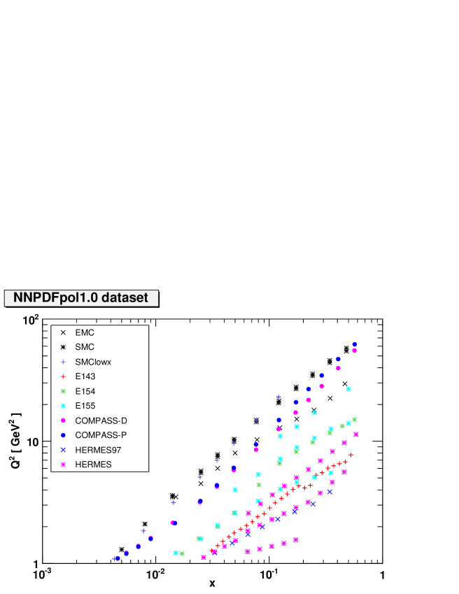
We have excluded from our analysis all data points with $Q^{2}\leq Q^{2}_{\rm cut}=1$ GeV², since below such energy scale perturbative QCD cannot be considered reliable. A similar choice of cut was made in Refs. [6, 7, 8, 15, 11, 12]. We further impose a cut on the squared invariant mass of the hadronic final state $W^{2}=Q^{2}(1-x)/x$ in order to remove points which may be affected by sizable higher-twist corrections. The cut is chosen based on a study presented in Ref. [50], where higher twist terms were added to the observables, with a coefficient fitted to the data, and it was shown that the higher twist contribution becomes compatible with zero if one imposes the cut $W^{2}\geq W^{2}_{\rm cut}=6.25$ GeV². We will follow this choice, which excludes data points with large Bjorken-$x$ at moderate values of the squared momentum transfer $Q^{2}$, roughly corresponding to the bottom-right corner of the $(x,Q^{2})$-plane, see Fig. 1: in particular, it excludes all available JLAB data [51, 52, 53]. The number of data points surviving the kinematic cuts for each data set is given in parenthesis in Tab. 1.

As can be seen from the scatter plot in Fig. 1, the region of the $(x,Q^{2})$-plane where data are available after kinematic cuts is roughly restricted to $4\cdot 10^{-3}\lesssim x\lesssim 0.6$ and $1$ GeV${}^{2}\leq Q^{2}\lesssim 60$ GeV². In recent years, the coverage of the low-$x$ region has been improved by a complementary set of SMC data [42] and by the more recent COMPASS data [45, 46]. In the large-$x$ region, information is provided at rather high $Q^{2}$ by the same COMPASS data and at lower energy by the latest HERMES measurements [48]. In comparison to the dataset used in Refs. [6, 7, 8] several new datasets are being used, in particular the SMC [42], HERMES [48] and COMPASS [45, 46] data. The dataset used in this paper is the same as that of Ref. [11], and also the same as the DIS data of the fit of Ref. [15], which however has a wider data set which extends beyond inclusive DIS.

Each experimental collaboration provides uncertainties on the measured quantities listed in the next-to-last column of Tab. 1. Correlated systematics are only provided by EMC and E143, which give the values of the systematics due to the uncertainty in the beam and target polarizations, while all other experiments do not provide any information on the covariance matrix. For each experiment, we determine the uncorrelated uncertainty on $g_{1}$ by combining the uncertainty on the experimental observable with that of the unpolarized structure function using standard error propagation. We include all available correlated systematics. These are provided by the experimental collaboration as a percentage correction to $g_{1}$ (or, alternatively, to the asymmetry $A_{1}$): we apply the percentage uncertainty on $g_{1}$ to the structure function determined by us as discussed in Sect. 2.2 (which, of course, is very close to the value determined by the experimental collaboration).

We then construct a covariance matrix

$${\rm cov}_{pq}=\left(\sum_{i}\sigma^{(c)}_{i,p}\sigma^{(c)}_{i,q}+\delta_{pq}\sigma^{(u)}_{p}\sigma^{(u)}_{q}\right)g_{1,p}g_{1,q},$$ (23)

where $p$ and $q$ run over the experimental data points, $g_{1,p}\equiv g_{1}(x_{p},Q_{p}^{2})$ ($g_{1,q}\equiv g_{1}(x_{q},Q_{q}^{2})$), $\sigma^{(c)}_{i,p}$ are the various sources of correlated uncertainty, and $\sigma^{(u)}_{p}$ the uncorrelated uncertainties, which are in turn found as a sum in quadrature of all uncorrelated sources of statistical $\sigma^{\rm(stat)}_{i,p}$ and systematic $\sigma^{\rm(syst)}_{i,p}$ uncertainty on each point:

$$\left(\sigma^{(u)}_{p}\right)^{2}=\sum_{i}\left(\sigma^{\rm(stat)}_{i,p}\right)^{2}+\sum_{j}\left(\sigma^{\rm(syst)}_{j,p}\right)^{2}.$$ (24)

The correlation matrix is defined as

$$\rho_{pq}=\frac{{\rm cov}_{pq}}{\sigma^{\rm(tot)}_{p}\sigma^{\rm(tot)}_{q}g_{1,p}g_{1,q}}\mbox{ ,}$$ (25)

where the total uncertainty $\sigma^{\rm(tot)}_{p}$ on the $p$-th data point is

$$\left(\sigma^{\rm(tot)}_{p}\right)^{2}=(\sigma^{(u)}_{p})^{2}+\sum_{i}\left(\sigma^{(c)}_{i,p}\right)^{2}\mbox{ .}$$ (26)

We show in Tab. 2 the average experimental uncertainties for each dataset, with uncertainties separated into statistical and correlated systematics. All values are given as absolute uncertainties and refer to the structure function $g_{1}$, which has been reconstructed for each experiment as discussed above. As in the case of Tab. 1, we provide the values before and after kinematic cuts (if different).

In Tab. 1, we distinguish between experiments, defined as groups of data which cannot be correlated to each other, and datasets within a given experiment, which could in principle be correlated with each other, as they correspond to measurements of different observables in the same experiment, or measurements of the same observable in different years. Even though, in practice, only two experiments provide such correlated systematics (see Tab. 2), this distinction will be useful in the minimization strategy, see Sect. 4 below.

Experiment	Set	$\langle\delta{g_{1}}_{\mbox{\tiny s}}\rangle$	$\langle\delta{g_{1}}_{\mbox{\tiny c}}\rangle$	$\langle\delta{g_{1}}_{\mbox{\tiny tot}}\rangle$
EMC
	EMC-A1P	0.144	0.037	0.150
SMC
	SMC-A1P	0.098	–	0.098
	SMC-A1D	0.116	–	0.116
SMClowx
	SMClx-A1P	18.379 (0.291)	– (–)	18.379 (0.291)
	SMClx-A1D	22.536 (0.649)	– (–)	22.536 (0.649)
E143
	E143-A1P	0.042 (0.046)	0.009 (0.009)	0.043 (0.047)
	E143-A1D	0.053 (0.058)	0.004 (0.005)	0.054 (0.059)
E154
	E154-A1N	0.044	–	0.044
E155
	E155-G1P	0.040 (0.043)	– (–)	0.040 (0.043)
	E155-G1N	0.124 (0.135)	– (–)	0.124 (0.135)
COMPASS-D
	CMP07-A1D	0.061	–	0.061
COMPASS-P
	CMP10-A1P	0.101	–	0.101
HERMES97
	HER97-A1N	0.087 (0.093)	– (–)	0.087 (0.093)
HERMES
	HER-A1P	0.067 (0.062)	– (–)	0.067 (0.062)
	HER-A1D	0.040 (0.034)	– (–)	0.040 (0.034)

Table 2: Averaged statistical, correlated systematic and total uncertainties before and after (in parenthesis) kinematic cuts for each of the experimental sets included in the present analysis. Uncorrelated systematic uncertainties are considered as part of the statistical uncertainty and they are added in quadrature. All values are absolute uncertainties and refer to the structure function $g_{1}$, which has been reconstructed for each experiment as discussed in the text. Details on the number of points and the kinematics of each dataset are provided in Tab. 1.

2.3 Monte-Carlo generation of the pseudo-data sample

Error propagation from experimental data to the fit is handled by a Monte Carlo sampling of the probability distribution defined by data. The statistical sample is obtained by generating $N_{\mathrm{rep}}$ pseudodata replicas, according to a multigaussian distribution centered at the data points and with a covariance equal to that of the original data. Explicitly, given an experimental data point $g_{1,p}^{(\mathrm{exp})}\equiv g_{1}(x_{p},Q_{p}^{2})$, we generate $k=1,\dots,N_{\mathrm{rep}}$ artificial points $g_{1,p}^{(\mathrm{art}),(k)}$ according to

$$g_{1,p}^{(\mathrm{art}),(k)}(x,Q^{2})=\left[1+\sum_{i}r_{(c),p}^{(k)}\sigma_{i,p}^{(c)}+r_{(u),p}^{(k)}\sigma_{p}^{(u)}\right]g_{1,p}^{(\mathrm{exp})}(x,Q^{2}),$$ (27)

where $r_{(c),p}^{(k)}$, $r_{(u),p}^{(k)}$ are univariate gaussianly distributed random numbers, and $\sigma_{i,p}^{(c)}$ and $\sigma_{p}^{(u)}$ are respectively the relative correlated systematic and statistical uncertainty. Unlike in the unpolarized case, Eq. (27) receives no contribution from normalization uncertainties, given that all polarized observables are obtained as cross section asymmetries.

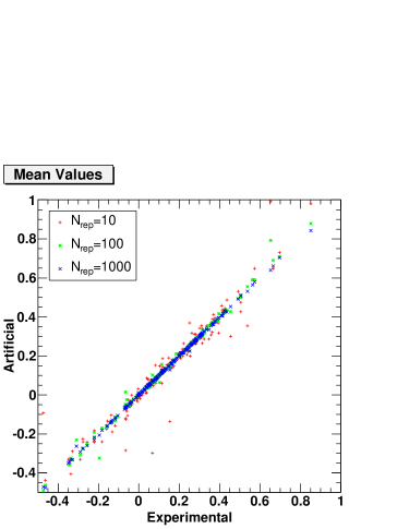
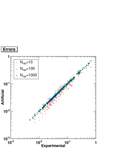
The number of Monte Carlo replicas of the data is determined by requiring that the central values, uncertainties and correlations of the original experimental data can be reproduced to a given accuracy by taking averages, variances and covariances over the replica sample. A comparison between expectation values and variances of the Monte Carlo set and the corresponding input experimental values as a function of the number of replicas is shown in Fig. 2, where we display scatter-plots of the central values and errors for samples of $N_{\mbox{\scriptsize{rep}}}=10,100$ and $1000$ replicas. A more quantitative comparison can be performed by defining suitable statistical estimators (see, for example, Appendix B of Ref. [18]).

We show in Tabs. 3–4 the percentage error and the scatter correlation $r$ (which is crudely speaking the correlation between the input value and the value computed from the replica sample) for central values and errors respectively . We do not compute values for correlations, as these, as seen in Tab. 2, are only available for a very small number of data points from two experiments. Note that some large values of the percentage uncertainty are due to the fact that $g_{1}$ for some experiments can take values which are very close to zero. It is clear from both the tables and the plots that a Monte Carlo sample of pseudo-data with $N_{\mathrm{rep}}=100$ is sufficient to reproduce the mean values and the errors of experimental data to an accuracy which is better than 5%, while the improvement in going up to $N_{\mathrm{rep}}=1000$ is moderate. Therefore, we will henceforth use a $N_{\mathrm{rep}}=100$ replica sample as a default in the remainder of this paper.

	Estimator	$\left\langle\mbox{PE}\left[\langle g_{1}^{\mbox{\scriptsize{(art)}}}\rangle\right]\right\rangle$ [%]			$r\left[g_{1}^{\mbox{\scriptsize{(art)}}}\right]$
	$N_{\mbox{\scriptsize{rep}}}$	10	100	1000	10	100	1000
Experiment	EMC	23.7	3.5	2.9	.76037	.99547	.99712
	SMC	19.4	5.6	1.2	.94789	.99908	.99993
	SMClowx	183	25.8	15.4	.80370	.99239	.99960
	E143	18.5	5.7	2.1	.99159	.99860	.99984
	E154	239	44.0	21.9	.99635	.99981	.99994
	E155	37.3	13.4	4.3	.99798	.99993	.99998
	COMPASS-D	26.4	8.6	3.2	.96016	.98774	.99917
	COMPASS-P	16.4	1.9	1.5	.91942	.99829	.99902
	HERMES97	22.5	6.2	2.2	.96168	.99762	.99979
	HERMES	10.5	5.8	1.2	.98564	.99916	.99973

Table 3: Table of statistical estimators for the mean value computed from the Monte Carlo sample with $N_{\mathrm{rep}}=10,100,1000$ replicas. Estimators refer to individual experiments and are defined in Appendix B of Ref. [18].

	Estimator	$\left\langle\mbox{PE}\left[\langle\delta g_{1}^{\mbox{\scriptsize{(art)}}}\rangle\right]\right\rangle$ [%]			$r\left[\delta g_{1}^{\mbox{\scriptsize{(art)}}}\right]$
	$N_{\mbox{\scriptsize{rep}}}$	10	100	1000	10	100	1000
Experiment	EMC	12.8	4.9	2.0	.97397	.99521	.99876
	SMC	22.4	5.4	1.7	.96585	.99489	.99980
	SMClowx	16.9	6.2	2.1	.97959	.99490	.99905
	E143	16.0	7.4	2.0	.95646	.98684	.99946
	E154	19.1	3.7	1.3	.99410	.99871	.99992
	E155	21.2	5.6	1.8	.99428	.99971	.99997
	COMPASS-D	15.5	5.2	1.6	.99375	.99687	.99993
	COMPASS-P	18.4	7.4	1.5	.99499	.99005	.99988
	HERMES97	17.9	6.4	1.6	.89065	.97318	.99894
	HERMES	19.5	6.0	1.6	.91523	.99237	.99942

Table 4: Table of statistical estimators for the errors computed from the Monte Carlo sample with $N_{\mathrm{rep}}=10,100,1000$ replicas. Estimators refer to individual experiments and are defined in Appendix B of Ref. [18].

Figure 2: Scatter-plot of experimental versus artificial Monte Carlo mean central values and absolute uncertainties of polarized structure functions computed from ensembles made of $N_{\mbox{\scriptsize{rep}}}=10,100,1000$ replicas.

3 From polarized PDFs to observables

3.1 Leading-twist factorization of the structure functions

At leading twist, the polarized structure function $g_{1}$ for neutral-current virtual photon DIS is given in terms of the polarized quark and gluon distributions by

$$g_{1}(x,Q^{2})=\frac{\langle e^{2}\rangle}{2}[C_{NS}\otimes\Delta q_{NS}+C_{S}\otimes\Delta\Sigma+2n_{f}C_{g}\otimes\Delta g]\ .$$ (28)

Here $n_{f}$ is the number of active flavors, the average charge is given by $\langle e^{2}\rangle=n_{f}^{-1}\sum_{i=1}^{n_{f}}e^{2}_{i}$ in terms of the electric charge $e_{i}$ of the $i$-th quark flavor, $\otimes$ denotes the convolution with respect to $x$, and the nonsinglet and singlet quark distributions are defined as

$$\Delta q_{NS}\equiv\sum_{i=1}^{n_{f}}\left(\frac{e^{2}_{i}}{\langle e^{2}\rangle}-1\right)(\Delta q_{i}+\Delta\bar{q}_{i}),\qquad\Delta\Sigma\equiv\sum_{i=1}^{n_{f}}(\Delta q_{i}+\Delta\bar{q}_{i}),$$ (29)

where $\Delta q_{i}$ and $\Delta\bar{q}_{i}$ are the polarized quark and antiquark distributions of flavor $i$ and $\Delta g$ is the polarized gluon PDF.

In the parton model, Eq. (28) reduces to

$$g_{1}(x,Q^{2})=\frac{1}{2}\sum_{i=1}^{n_{f}}e_{i}^{2}\left(\Delta q_{i}(x,Q^{2})+\Delta\bar{q}_{i}(x,Q^{2})\right),$$ (30)

but in perturbative QCD the parton model expression is not recovered even when $\alpha_{s}\to 0$ because at large $Q^{2}$ the first moment of the gluon distribution $\int_{0}^{1}\!dx\,\Delta g\sim({\alpha_{s}(Q^{2}))^{-1}}$, so the gluon does not decouple from $g_{1}$ asymptotically. Be that as it may, below charm threshold, with $n_{f}=3$, Eq. (28) can be rewritten as

$$g_{1}(x,Q^{2})=\frac{1}{9}\Delta\Sigma(x,Q^{2})+\frac{1}{12}\Delta T_{3}(x,Q^{2})+\frac{1}{36}\Delta T_{8}(x,Q^{2}),$$ (31)

in terms of the singlet quark-antiquark distribution $\Delta\Sigma(x,Q^{2})$, defined in Eq. (29), the isospin triplet combination

$$\Delta T_{3}(x,Q_{0}^{2})=\Delta u(x,Q_{0}^{2})+\Delta\bar{u}(x,Q_{0}^{2})-\left[\Delta d(x,Q_{0}^{2})+\Delta\bar{d}(x,Q_{0}^{2})\right],$$ (32)

and the SU(3) octet combination

$$\Delta T_{8}(x,Q_{0}^{2})=\Delta u(x,Q_{0}^{2})+\Delta\bar{u}(x,Q_{0}^{2})+\Delta d(x,Q_{0}^{2})+\Delta\bar{d}(x,Q_{0}^{2})-2\left[\Delta s(x,Q_{0}^{2})+\Delta\bar{s}(x,Q_{0}^{2})\right].$$ (33)

It is clear from Eqs. (28-30) that neutral current $g_{1}$ data only allow for a direct determination of the four polarized PDF combinations $\Delta g$, $\Delta\Sigma$, $\Delta T_{3}$ and $\Delta T_{8}$. In principle, an intrinsic polarized component could also be present for each heavy flavour. However, we will neglect it here and assume that heavy quark PDFs are dynamically generated above threshold by (massless) Altarelli-Parisi evolution, in a zero-mass variable-flavor number (ZM-VFNS) scheme. In such a scheme all heavy quark mass effects are neglected. While they can be introduced for instance through the FONLL method [54], these effects have been shown to be relatively small already on the scale of present-day unpolarized PDF uncertainties, and thus are most likely negligible in the polarized case where uncertainties are rather larger.

The proton and neutron PDFs are related to each other by isospin, which we will assume to be exact, thus yielding

$$\Delta u^{p}=\Delta d^{n},\quad\Delta d^{p}=\Delta u^{n},\quad\Delta s^{p}=\Delta s^{n},$$ (34)

and likewise for the polarized anti-quarks. In the following we will always assume that PDFs refer to the proton. The first moment of all non-singlet combinations of quark and antiquark distributions are scale-independent because of axial current conservation, while the first moment of the singlet quark distribution is not. Because of the axial anomaly, the first moment of the singlet quark distribution is scale-dependent in the $\overline{\rm MS}$ scheme. However, it may be convenient to choose a factorization scheme in which the first moment of the singlet quark distribution is also scale independent so that all the individual quark and antiquark spin fractions are scale independent. Several such schemes, including the so-called Adler-Bardeen (AB) scheme, were discussed in Ref. [6], where the transformation connecting them to the $\overline{\rm MS}$ scheme was constructed explicitly.

By means of the SU(2) or SU(3) flavour symmetry it is possible to relate the first moments of the nonsinglet $C$-even combinations ($\Delta T_{3}$ and $\Delta T_{8}$) to the baryon octet decay constants $a_{3}$ and $a_{8}$:

$$a_{3} =\int_{0}^{1}dx~{}\Delta T_{3}(x,Q^{2}),$$ (35)

$$a_{8} =\int_{0}^{1}dx~{}\Delta T_{8}(x,Q^{2}),$$ (36)

whose current experimental values are [55]

$$a_{3}=g_{A}=1.2701\pm 0.0025,$$ (37)

$$a_{8}=0.585\pm 0.025.$$ (38)

A much larger uncertainty on the octet axial charge, up to about 30%, is found if SU(3) symmetry is violated [56]. Even though a detailed phenomenological analysis does not seem to support this conclusion [57], we will take as default this more conservative uncertainty estimation

$$a_{8}=0.585\pm 0.176.$$ (39)

The impact of replacing this with the more aggressive determination given in Eq. (38) will be studied in Sect. 5.3.2.

Structure functions will be computed in terms of polarized parton distributions using the so-called NNPDF FastKernel method, introduced in Ref. [23]. In short, in this method the PDFs at scale $Q^{2}$ are obtained by convoluting the parton distributions at the parametrization scale $Q_{0}^{2}$ with a set of Green’s functions, which are in turn obtained by solving the QCD evolution equations in Mellin space. These Green’s functions are then convoluted with coefficient functions, so that the structure function can be directly expressed in terms of the PDFs at the parametrization scale through suitable kernels $K$. In terms of the polarized PDFs at the input scale we have

$$g_{1}^{p}=\{K_{{\rm g1},\Delta\Sigma}\otimes\Delta\Sigma_{0}+K_{{\rm g1},\Delta g}\otimes\Delta g_{0}+K_{{\rm g1},+}\otimes\left(\Delta T_{3,0}+\hbox{${{1}\over{3}}$}\Delta T_{8,0}\right)\}\ ,$$ (40)

where the kernels $K_{{\rm g1},\Delta\Sigma},K_{{\rm g1},\Delta g},K_{{\rm g1},+}$ take into account both the coefficient functions and $Q^{2}$ evolution. This way of expressing structure functions is amenable to numerical optimization, because all kernels can then be precomputed and stored, and convolutions may be reduced to matrix multiplications by projecting onto a set of suitable basis functions.

The neutron polarized structure function $g_{1}^{n}$ is given in terms of the proton and deuteron ones as

$$g_{1}^{n}=2\frac{g_{1}^{d}}{1-1.5\omega_{D}}-g_{1}^{p}\ ,$$ (41)

with $\omega_{D}=0.05$ the probability that the deuteron is found in a D state. Under the assumption of exact isospin symmetry, the expression of $g_{1}^{n}$ in terms of parton densities is obtained from Eq. (40) by interchanging the up and down quark PDFs, which amounts to changing the sign of $\Delta T_{3}$.

The implementation of the polarized PDF evolution up to NLO has been benchmarked against the HOPPET evolution code [58] using the settings of the Les Houches PDF evolution benchmark tables [59]. This benchmarking is discussed in more detail in Appendix A. We will assume the values $\alpha_{s}\left(M_{Z}^{2}\right)=0.119$ for the strong coupling constant and $m_{c}=1.4$ GeV and $m_{b}=4.75$ GeV for the charm and bottom quark masses respectively.

3.2 Target mass corrections to $g_{1}$

The leading twist expressions of structure functions given in Sect. 3.1 are corrected both by dynamical and kinematic higher-twist terms. The former are related to the contribution of higher twist operators to the Wilson expansion, and are generally expected to be small. The latter are related to target-mass corrections (TMCs), and because of their kinematical origin they can be included exactly: we do this following Ref. [60]. As discussed in Sect. 2.1, we thus consistently include all nucleon mass effects, both in the relation between measured asymmetries and structure functions, and in the relation between the latter and parton distributions.

The target mass corrections are especially simple in Mellin space, where they take the form [60]

$$\tilde{g}_{1}(N,Q^{2})=g_{1}(N,Q^{2})+\frac{m^{2}}{Q^{2}}\frac{N(N+1)}{(N+2)^{2}}\left[(N+4)~{}g_{1}(N+2,Q^{2})+4\frac{N+2}{N+1}~{}g_{2}(N+2,Q^{2})\right]+{\mathcal{O}}\left(\frac{m^{2}}{Q^{2}}\right)^{2}\ ,$$

(42)

$$\tilde{g}_{2}(N,Q^{2})=g_{2}(N,Q^{2})+\frac{m^{2}}{Q^{2}}\frac{N(N-1)}{(N+2)^{2}}\left[N\frac{N+2}{N+1}g_{2}(N+2,Q^{2})-g_{1}(N+2,Q^{2})\right]+{\mathcal{O}}\left(\frac{m^{2}}{Q^{2}}\right)^{2}\ .$$ (43)

We denote by $\tilde{g}_{1,2}(N,Q^{2})$ the Mellin space structure functions with TMCs included, while $g_{1,2}(N,Q^{2})$ are the structure functions determined in the $m=0$ limit.

As discussed in Sect. 2.1, in the absence of precise data on the structure function $g_{2}$, we will either determine it using the Wandzura-Wilczek approximation Eq. (22) (which is uncorrected by target-mass effects [60]), or, as a cross-check, simply setting it to zero. In either case, we may then determine $\tilde{g}_{1}$ Eq.(42) in terms of $g_{1}$.

In the former (Wandzura-Wilczek) case, substituting Eq. (21) in Eq. (42) and taking the inverse Mellin transform, we get

$$\tilde{g}_{1}(x,Q^{2})=\frac{1}{2\pi i}\int dN\,x^{-N}\left[1+\frac{m^{2}x^{2}}{Q^{2}}\frac{(N-2)^{2}(N-1)}{N^{2}}\right]g_{1}(N,Q^{2})\ ,$$ (44)

where we have shifted $N\to N-2$ in the term proportional to $m^{2}$. Inverting the Mellin transform we then obtain

$$\tilde{g}_{1}(x,Q^{2})=g_{1}(x,Q^{2})+\frac{m^{2}x^{2}}{Q^{2}}\left[-5g_{1}(x,Q^{2})-x\frac{dg_{1}(x,Q^{2})}{dx}+\int_{x}^{1}\frac{dy}{y}\left(8g_{1}(y,Q^{2})+4g_{1}(y,Q^{2})\log\frac{x}{y}\right)\right]\ .$$ (45)

If instead $g_{2}=0$,

$$\tilde{g}_{1}(x,Q^{2})=\frac{1}{2\pi i}\int dN\,x^{-N}\left[1+\frac{m^{2}x^{2}}{Q^{2}}\frac{(N^{2}-4)(N-1)}{N^{2}}\right]g_{1}(N,Q^{2})\ ,$$ (46)

whence

$$\tilde{g}_{1}(x,Q^{2})=g_{1}(x,Q^{2})+\frac{m^{2}x^{2}}{Q^{2}}\left[-g_{1}(x,Q^{2})-x\frac{dg_{1}(x,Q^{2})}{dx}-\int_{x}^{1}\frac{dy}{y}\left(4g_{1}(y,Q^{2})+4g_{1}(y,Q^{2})\log\frac{x}{y}\right)\right].$$ (47)

The numerical implementation of Eqs. (45) or Eq. (47) is difficult, because of the presence of the first derivative of $g_{1}$ in the correction term. Therefore, we will include target mass effects in an iterative way: we start by performing a fit in which we set $m=0$ and at each iteration the target mass corrected $g_{1}$ structure function is computed by means of Eqs. (45–47) using the $g_{1}$ obtained in the previous minimization step.

4 Neural networks and fitting strategy

We will now briefly review the NNPDF methodology for parton parametrization in terms of neural networks, and their optimization (fitting) through a genetic algorithm. The details of the procedure have been discussed in previous NNPDF papers, in particular Refs. [20, 23, 61]. Here we summarize the main steps of the whole strategy, and discuss in greater detail some points which are specific to the polarized case.

4.1 Neural network parametrization

Each of the independent polarized PDFs in the evolution basis introduced in Sect. 3.1, $\Delta\Sigma,\Delta g,\Delta T_{3}$ and $\Delta T_{8}$, is parametrized using a multi-layer feed-forward neural network [27]. All neural networks have the same architecture, namely 2-5-3-1, which corresponds to 37 free parameters for each PDF, and thus a total of 148 free parameters. This is to be compared to about 10-15 free parameters for all other available determinations of polarized PDFs. This parametrization has been explicitly shown to be redundant in the unpolarized case, in that results are unchanged when a smaller neural network architecture is adopted: this ensures that results do not depend on the architecture [27]. Given that polarized data are much less abundant and affected by much larger uncertainties than unpolarized ones, this architecture is adequate also in the polarized case.

The neural network parametrization is supplemented with a preprocessing function. In principle, large enough neural networks can reproduce any functional form given sufficient training time. However, the training can be made more efficient by adding a preprocessing step, i.e. by multiplying the output of the neural networks by a fixed function. The neural network then only fits the deviation from this function, which improves the speed of the minimization procedure if the preprocessing function is suitably chosen. We thus write the input PDF basis in terms of preprocessing functions and neural networks ${\rm NN}_{\rm\Delta pdf}$ as follows

$$\Delta\Sigma(x,Q_{0}^{2}) = {(1-x)^{m_{1}}}{x^{-n_{1}}}{\rm NN}_{\Delta\Sigma}(x)\ ,$$

$$\Delta T_{3}(x,Q_{0}^{2}) = A_{3}{(1-x)^{m_{3}}}{x^{-n_{3}}}{\rm NN}_{\Delta T_{3}}(x)\ ,$$

$$\Delta T_{8}(x,Q_{0}^{2}) = A_{8}{(1-x)^{m_{8}}}{x^{-n_{\Delta T_{8}}}}{\rm NN}_{\Delta T_{3}}(x)\ ,$$ (48)

$$\Delta g(x,Q_{0}^{2}) = {(1-x)^{m_{g}}}{x^{-n_{g}}}{\rm NN}_{\Delta g}(x).$$

Of course, one should check that no bias is introduced in the choice of preprocessing functions. To this purpose, we first select a reasonable range of values for the large and small–$x$ preprocessing exponents $m$ and $n$, and produce a PDF determination by choosing for each replica a value of the exponents at random with uniform distribution within this range. We then determine effective exponents for each replica, defined as

$$m_{\rm eff}(Q^{2})\equiv\lim_{x\to 1}\frac{\ln\Delta f(x,Q^{2})}{\ln(1-x)}\mbox{ ,}$$ (49)

$$n_{\rm eff}(Q^{2})\equiv\lim_{x\to 0}\frac{\ln\Delta f(x,Q^{2})}{\ln\frac{1}{x}}\mbox{ ,}$$ (50)

where $\Delta f=\Delta\Sigma\mbox{, }\Delta T_{3}\mbox{, }\Delta T_{8}\mbox{, }\Delta g$. Finally, we check that the range of variation of the preprocessing exponents is wider than the range of effective exponents for each PDF. If it is not, we enlarge the range of variation of preprocessing, then repeat the PDF determination, and iterate until the condition is satisfied. This ensures that the range of effective large- and small-$x$ exponents found in the fit is not biased, and in particular not restricted, by the range of preprocessing exponents. Our final values for the preprocessing exponents are summarized in Tab. 5, while the effective exponents obtained in our fit will be discussed in Sect. 5.5. It is apparent from Tab. 5 that the allowed range of preprocessing exponents is rather wider than in the unpolarized case, as a consequence of the limited amount of experimental information. It is enough to perform this check at the input evolution scale, $Q_{0}^{2}=1$ GeV².

PDF	$m$	$n$
$\Delta\Sigma(x,Q_{0}^{2})$	$\left[1.5,3.5\right]$	$\left[0.2,0.7\right]$
$\Delta g(x,Q_{0}^{2})$	$\left[2.5,5.0\right]$	$\left[0.4,0.9\right]$
$\Delta T_{3}(x,Q_{0}^{2})$	·$\left[1.5,3.5\right]$	$\left[0.4,0.7\right]$
$\Delta T_{8}(x,Q_{0}^{2})$	·$\left[1.5,3.0\right]$	$\left[0.1,0.6\right]$

Table 5: Ranges for the small and large $x$ preprocessing exponents Eq. (4.1).

Two of the PDFs in the parametrization basis Eq. (4.1), namely the nonsinglet triplet and octet $\Delta T_{3}$ and $\Delta T_{8}$, are supplemented by a prefactor. This is because these PDFs must satisfy the sum rules Eqs. (35, 36), which are enforced by letting

$$A_{3} = \frac{a_{3}}{\int_{0}^{1}dx\,(1-x)^{m_{3}}x^{-n_{3}}{\rm NN}_{\Delta T_{3}}(x)},$$

$$A_{8} = \frac{a_{8}}{\int_{0}^{1}dx\,(1-x)^{m_{8}}x^{-n_{8}}{\rm NN}_{\Delta T_{8}}(x)}.$$ (51)

The integrals are computed numerically each time the parameters of the PDF set are modified. The values of $a_{3}$ and $a_{8}$ are chosen for each replica as gaussianly distributed numbers, with central value and width given by the corresponding experimental values, Eqs. (37,39).

4.2 Genetic algorithm minimization

As discussed at length in Ref. [20], minimization with a neural network parametrization of PDFs must be performed through an algorithm which explores the very wide functional space efficiently. This is done by means of a genetic algorithm, which is used to minimize a suitably defined figure of merit, namely the error function [20],

$$E^{(k)}=\frac{1}{N_{\mathrm{dat}}}\sum_{I,J=1}^{N_{\rm dat}}\left(g_{I}^{(\mathrm{art})(k)}-g_{I}^{(\mathrm{net})(k)}\right)\left(\left({\mathrm{cov}}\right)^{-1}\right)_{IJ}\left(g_{J}^{(\mathrm{art})(k)}-g_{J}^{(\mathrm{net})(k)}\right)\ .$$ (52)

Here $g_{I}^{\rm(art)(k)}$ is the value of the observable $g_{I}$ at the kinematical point $I$ corresponding to the Monte Carlo replica $k$, and $g_{I}^{(\rm net)(k)}$ is the same observable computed from the neural network PDFs; the covariance matrix $\left({\rm cov}\right)_{IJ}$ is defined in Eq. (23).

The minimization procedure we adopt follows closely that of Ref. [19], to which we refer for a more general discussion. Minimization is perfomed by means of a genetic algorithm, which minimizes the figure of merit, Eq. (52) by creating, at each minimization step, a pool of new neural nets, obtained by randomly mutating the parameters of the starting set, and retaining the configuration which corresponds to the lowest value of the figure of merit.

The parameters which characterize the behaviour of the genetic algorithm are tuned in order to optimize the efficiency of the minimization procedure: here, we rely on previous experience of the development of unpolarized NNPDF sets. In particular, the algorithm is characterized by a mutation rate, which we take to decrease as a function of the number of iterations $N_{\rm ite}$ of the algorithm according to [20]

$$\eta_{i,j}=\eta_{i,j}^{(0)}/N_{\rm ite}^{r_{\eta}}\ ,$$ (53)

so that in the early stages of the training large mutations are allowed, while they become less likely as one approaches the minimum. The starting mutation rates are chosen to be larger for PDFs which contain more information. We perform two mutations per PDF at each step, with the starting rates given in Tab. 6. The exponent $r_{\eta}$ has been introduced in order to optimally span the whole range of possible beneficial mutations and it is randomized between $0$ and $1$ at each iteration of the genetic algorithm, as in Ref. [23].

Furthermore, following Ref. [23], we let the number of new candidate solutions depend on the stage of the minimization. At earlier stages of the minimization, when the number of generations is smaller than $N^{\rm mut}$, we use a large population of mutants, $N_{\rm mut}^{a}\gg 1$, so a larger space of mutations is being explored. At later stages of the minimization, as the minimum is approached, a smaller number of mutations $N_{\rm mut}^{b}\ll N_{\rm mut}^{a}$ is used. The values of the parameters $N_{\rm gen}^{\rm mut}$, $N_{\rm mut}^{a}$ and $N_{\rm mut}^{b}$ are collected in Tab. 7.

$\eta^{(0)}_{i,\Delta\Sigma}$	$\eta^{(0)}_{i,\Delta g}$	$\eta^{(0)}_{i,\Delta T_{3}}$	$\eta^{(0)}_{i,\Delta T_{8}}$
$5,0.5$	$5,0.5$	$2,0.2$	$2,0.2$

Table 6: The initial values of the mutation rates for the two mutations of each PDF.

$N_{\rm gen}^{\rm mut}$	$N^{a}_{\rm mut}$	$N^{b}_{\rm mut}$	$N_{\rm gen}^{\rm wt}$	$E^{\mathrm{sw}}$
200	50	10	5000	2.5

Table 7: Values of the parameters of the genetic algorithm.

Because the minimization procedure stops the fit to all experiments at once, we must make sure that the quality of the fit to different experiments is approximately the same. This is nontrivial, because of the variety of experiments and datasets included in the fit. Therefore, the figure of merit per datapoint for a given set is not necessarily a reliable indicator of the quality of the fit to that set, because some experiments may have systematically underestimated or overestimated uncertainties. Furthermore, unlike for unpolarized PDF fits, information on the experimental covariance matrix is only available for a small subset of experiments, so for most experiments statistical and systematic errors must be added in quadrature, thereby leading to an overestimate of uncertainties: this leads to a wide spread of values of the figure of merit, whose value depends on the size of the correlated uncertainties which are being treated as uncorrelated.

A methodology to deal with this situation was developed in Ref. [23]. The idea is to first determine the optimal value of the figure of merit for each experiment, i.e. a set of target values $E_{i}^{\rm targ}$ for each of the $i$ experiments, then during the fit give more weight to experiments for which the figure of merit is further away from its target value, and stop training experiments which have already reached the target value. This is done by minimizing, instead of the figure of merit Eq. (52), the weighted figure of merit

$$E_{\rm wt}^{(k)}=\frac{1}{N_{\mathrm{dat}}}\sum_{j=1}^{N_{\mathrm{sets}}}p_{j}^{(k)}N_{\mathrm{dat},j}E_{j}^{(k)}\,,$$ (54)

where $E_{j}^{(k)}$ is the error function for the $j$-th dataset with $N_{{\rm dat},j}$ points, and the weights $p_{j}^{(k)}$ are given by

1. If $E_{i}^{(k)}\geq E_{i}^{\rm targ}$, then $p_{i}^{(k)}=\left(E_{i}^{(k)}/E_{i}^{\rm targ}\right)^{n}$,

2. If $E_{i}^{(k)}<E_{i}^{\rm targ}$, then $p_{i}^{(k)}=0$  ,

with $n$ a free parameter which essentially determines the amount of weighting. In the unpolarized fits of Refs. [23, 25, 26, 29] the value $n=2$ was used. Here instead we will choose $n=3$. This larger value, determined by trial and error, is justified by the wider spread of figures of merit in the polarized case, which in turn is related to the absence of correlated systematics for most experiments.

The target values $E_{i}^{\rm targ}$ are determined through an iterative procedure: they are set to one at first, then a very long fixed-length fit is run, and the values of $E_{i}$ are taken as targets for a new fit, which is performed until stopping (according to the criterion to be discussed in Sect. 4.3 below). The values of $E_{i}$ at the end of this fit are then taken as new targets until convergence is reached, usually after a couple iterations.

Weighted training stops after the first $N_{\rm gen}^{\rm wt}$ generations, unless the total error function Eq. (52) is above some threshold $E^{(k)}\geq E^{\rm sw}$. If it is, weighted training continues until $E^{(k)}$ falls below the threshold value. Afterwards, the error function is just the unweighted error function Eq. (52) computed on experiments. This ensures that the figure of merit behaves smoothly in the last stages of training. The values for the parameters $N_{\rm gen}^{\rm wt}$ and $E^{\rm sw}$ are also given in Tab. 7.

4.3 Determination of the optimal fit

Because the neural network parametrization is very redundant, it may be able to fit not only the underlying behaviour of the PDFs, but also the statistical noise in the data. Therefore, the best fit does not necessarily coincide with the absolute minimum of the figure of merit Eq. (52). We thus determine the best fit, as in Refs. [19, 20], using a cross-validation method [62]: for each replica, the data are randomly divided in two sets, training and validation, which include a fraction $f_{\rm tr}^{(j)}$ and $f_{\rm val}^{(j)}=1-f_{\rm tr}^{(j)}$ of the data points respectively. The figure of merit Eq. (52) is then computed for both sets. The training figure of merit function is minimized through the genetic algorithm, while the validation figure of merit is monitored: when the latter starts increasing while the former still decreases the fit is stopped. This means that the fit is stopped as soon as the neural network is starting to learn the statistical fluctuations of the points, which are different in the training and validation sets, rather than the underlying law which they share.

In the unpolarized fits of Refs. [19, 20, 23, 25, 26, 29] equal training and validation fractions were uniforlmly chosen, $f_{\rm tr}^{(j)}=f_{\rm val}^{(j)}=1/2$. However, in this case we have to face the problem that the number of datapoints is quite small: most experiments include about ten datapoints (see Tab. 1). Hence, it is difficult to achieve a stable minimization if only half of them are actually used for minimization, as we have explicitly verified. Therefore, we have chosen to include 80% of the data in the training set, i.e. $f_{\rm tr}^{(j)}=0.8$ and $f_{\rm val}^{(j)}=0.2$. We have explicitly verified that the fit quality which is obtained in this case is comparable to the one achieved when including all data in the training set (i.e. with $f_{\rm tr}^{(j)}=1.0$ and $f_{\rm val}^{(j)}=0.0$), but the presence of a nonzero validation set allows for a satisfactory stopping, as we have checked by explicit inspection of the profiles of the figure of merit as a function of training time.

In practice, in order to implement cross-validation we must determine a stopping criterion, namely, give conditions which must be satisfied in order for the minimization to stop. First, we require that the weighted training stage has been completed, i.e., that the genetic algorithm has been run for at least $N_{\rm gen}^{\rm wt}$ minimization steps. Furthermore, we check that all experiments have reached a value of the figure of merit below a minimal threshold $E_{\rm thr}$. Note that because stopping can occur only after weighted training has been switched off, and this in turn only happens when the figure of merit falls below the value $E^{\rm sw}$, the total figure of merit must be below this value in order for stopping to be possible.

We then compute moving averages

$$\langle E_{\mathrm{tr,val}}(i)\rangle\equiv\frac{1}{N_{\mathrm{smear}}}\sum_{l=i-N_{\mathrm{smear}}+1}^{i}E_{\mathrm{wt;\,tr,val}}(l)\,,$$ (55)

of the figure of merit Eq. (54) for either the training or the validation set at the $l$-th genetic minimzation step. The fit is then stopped if

$$r_{\rm tr}<1-\delta_{\rm tr}\quad{\rm and}\quad r_{\rm val}>1+\delta_{\rm val}\,,$$ (56)

where

$$r_{\rm tr}\equiv\frac{\langle E_{\mathrm{tr}}(i)\rangle}{\langle E_{\mathrm{tr}}(i-\Delta_{\mathrm{smear}})\rangle}\,,$$ (57)

$$r_{\rm val}\equiv\frac{\langle E_{\mathrm{val}}(i)\rangle}{\langle E_{\mathrm{val}}(i-\Delta_{\mathrm{smear}})\rangle}\,.$$ (58)

The parameter $N_{\rm smear}$ determines the width of the moving average; the parameter $\Delta_{\rm smear}$ determines the distance between the two points along the minimization path which are compared in order to determine whether the figure of merit is increasing or decreasing; and the parameters $\delta_{\rm tr}$, $\delta_{\rm val}$ are the threshold values for the decrease of the training and increase of the validation figure of merit to be deemed significant. The optimal value of these parameters should be chosen in such a way that the fit does not stop on a statistical fluctuation, yet it does stop before the fit starts overlearning (i.e. learning statistical fluctuation). As explained in Ref. [23], this is done studying the profiles of the error functions for individual dataset and for individual replicas. In order to avoid unacceptably long fits, training is stopped anyway when a maximum number of iterations $N_{\rm gen}^{\rm max}$ is reached, even though the stopping conditions Eq. (56) are not satisfied. This leads to a small loss of accuracy of the corresponding fits: this is acceptable provided it only happens for a small enough fraction of replicas. If a fit stops at $N_{\rm gen}^{\rm max}$ without the stopping criterion having been satisfied, we also check that the total figure of merit is below the value $E^{\rm sw}$ at which weighted training is switched off. If it hasn’t, we conclude that the specific fit has not converged, and we retrain the same replica, i.e., we perform a new fit to the same data starting with a different random seed. This only occurs in about one or two percent of cases.

The full set of parameters which determine the stopping criterion is given in Tab. 8.

$N_{\rm gen}^{\rm max}$	$E_{\rm thr}$	$N_{\rm smear}$	$\Delta_{\rm smear}$	$\delta_{\rm tr}$	$\delta_{\rm val}$
$20000$	$8$	$100$	$100$	$5\cdot 10^{-4}$	$5\cdot 10^{-4}$

Table 8: Parameters for the stopping criterium.

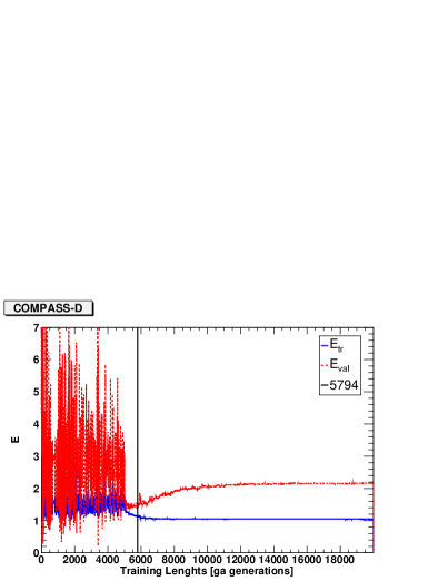
An example of how the stopping criterium works in practice is shown in Fig. 3. We display the moving averages Eq. (55) of the training and validation error functions $\langle E_{\rm tr,val}^{(k)}\rangle$, computed with the parameter settings of Tab. 8, and plotted as a function of the number of iterations of the genetic algorithm, for a particular replica and for two of the experiments included in the fit. The wide fluctuations which are observed in the first part of training, up to the $N_{\rm gen}^{\rm wt}$-th generation, are due to the fact that the weights which enter the definition of the figure of merit Eq. (54) are frequently adjusted. Nevertheless, the downwards trend of the figure of merit is clearly visible. Once the weighted training is switched off, minimization proceeds smoothly. The vertical line denotes the point at which the stopping criterion is satisfied. Here, we have let the minimization go on beyond this point, and we see clearly that the minimization has entered an overlearning regime, in which the validation error function $E_{\rm val}^{(k)}$ is rising while the training $E_{\rm tr}^{(k)}$ is still decreasing. Note that the stopping point, which in this particular case occurs at $N_{\rm gen}^{\rm stop}=5794$, is determined by verifying that the stopping criteria are satisfied by the total figure of merit, not that of individual experiments shown here. The fact that the two different experiments considered here both start overlearning at the same point shows that the weighted training has been effective in synchronizing the fit quality for different experiments.

Figure 3: Behaviour of the moving average Eq. (55) of the training and validation figure of merit for two different datasets included in a global fit (COMPASS-P and HERMES) as a function of training length. The The straight vertical line indicates the point at which the fit stops with the stopping parameters of Tab. 8. The weighted training is switched off at $N_{\rm gen}^{\rm wt}=5000$.

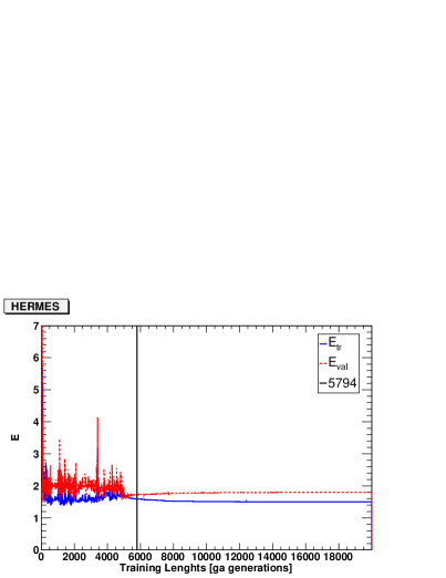
4.4 Theoretical constraints

Polarized PDFs are only loosely constrained by data, which are scarce and not very accurate. Theoretical constraints are thus especially important in reducing the uncertainty on the PDFs. We consider in particular positivity and integrability.

Positivity of the individual cross sections which enter the polarized asymmetries Eq. (1) implies that, up to power-suppressed corrections, longitudinal polarized structure functions are bounded by their unpolarized counterparts, i.e.

$$|g_{1}(x,Q^{2})|\leq F_{1}(x,Q^{2}).$$ (59)

At leading order, structure functions are proportional to parton distributions, so imposing Eq. (59) for any process (and a similar condition on an asymmetry which is sensitive to polarized gluons [63]), would imply

$$|\Delta f_{i}(x,Q^{2})|\leq f_{i}(x,Q^{2})$$ (60)

for any pair of unpolarized and polarized PDFs $f$ and $\Delta f$, for all quark flavors and gluon $i$, for all $x$, and for all $Q^{2}$. Beyond leading order, the condition Eq. (59) must still hold, but it does not necessarily imply Eq. (60). Rather, one should then impose at least a number of conditions of the form of Eq. (59) on physically measurable cross-sections which is equal to the number of independent polarized PDFs. For example, in principle one may require that the condition Eq. (59) is separately satisfied for each flavor, i.e. when only contributions from the $i$-th flavor are included in the polarized and unpolarized structure function: this corresponds to requiring positivity of semi-inclusive structure functions which could in principle be measured (and that fragmentation effects cancel in the ratio). A condition on the gluon can be obtained by imposing positivity of the polarized and unpolarized cross-sections for inclusive Higgs production in gluon-proton scattering [63], again measurable in principle if not in practice.

Because $g_{1}/F_{1}\sim x$ as $x\to 0$ [64], the positivity bound Eq. (59) is only significant at large enough $x\gtrsim 10^{-2}$. On the other hand, at very large $x$ the NLO corrections to the LO positivity bound become negligible [63, 65]. Therefore, the NLO positivity bound in practice only differs from its LO counterpart Eq. (60) in a small region $10^{-2}\sim x\lesssim 0.3$, and even there by an amount of rather less that 10% [63], which is negligible in comparison to the size of PDF uncertainties, as we shall see explicitly in Sec. 5.

Therefore, we will impose the leading-order positivity bound Eq. (60) on each flavor combination $\Delta q_{i}+\Delta\bar{q}_{i}$ and on the gluon $\Delta g$ (denoted as $\Delta f_{i}$ below). We do this by requiring

$$|\Delta f_{i}(x,Q^{2})|\leq f_{i}(x,Q^{2})+\sigma_{i}(x,Q^{2})\ ,$$ (61)

where $\sigma_{i}(x,Q^{2})$ is the uncertainty on the corresponding unpolarized PDF combination $f_{i}(x,Q^{2})$ at the kinematic point $(x,Q^{2})$. This choice is motivated by two considerations. First, it is clearly meaningless to impose positivity of the polarized PDF to an accuracy which is greater than that with which the unpolarized PDF has been determined. Second, because the unpolarized PDFs satisfy NLO positivity, they can become negative and thus they may have nodes. As a consequence, the LO bound Eq. (60) would imply that the polarized PDF must vanish at the same point, which would be clearly meaningless.

As in Ref. [23] positivity is imposed during the minimization procedure, thereby guaranteeing that the genetic algorithm only explores the subspace of acceptable physical solutions. This is done through a Lagrange multiplier $\lambda_{\rm pos}$, i.e. by computing the polarized PDF at $N_{\rm dat,pos}$ fixed kinematic points $(x_{p},Q_{0}^{2})$ and then adding to the error function Eq. (52) a contribution

$$E_{\rm pos}^{(k)}={\lambda_{\rm pos}}\sum_{p=1}^{N_{\rm dat,pos}}\Bigg{\{}\sum_{j=u+\bar{u},d+\bar{d},s+\bar{s},g}\Theta\left[\left|\Delta f_{j}^{(\rm net)(k)}(x_{p},Q_{0}^{2})\right|-\left(f_{j}+\sigma_{j}\right)(x_{p},Q_{0}^{2})\right]$$

$$\qquad\qquad\times\left[\left|\Delta f_{j}^{(\rm net)(k)}(x_{p},Q_{0}^{2})\right|-\left(f_{j}+\sigma_{j}\right)(x_{p},Q_{0}^{2})\right]\Bigg{\}}\ .$$ (62)

This provides a penalty, proportional to the violation of positivity, which enforces Eq. (61) separately for all the non-zero quark-antiquark combinations. The values of the unpolarized PDF combination $f_{j}(x,Q^{2})$ and its uncertainty $\sigma_{j}(x,Q^{2})$ are computed using the NNPDF2.1 NNLO PDF set [25], while $\Delta f_{j}^{(\rm net)(k)}$ is the corresponding polarized PDF computed from the neural network parametrization for the $k$-th replica. The polarized and unpolarized PDFs are evaluated at $N_{\rm dat,pos}=20$ points with $x$ equally spaced in the interval

$$x\in\left[10^{-2},0.9\right]\ .$$ (63)

Positivity is imposed at the initial scale $Q_{0}^{2}=1$ GeV² since once positivity is enforced at low scales, it is automatically satisfied at larger scales [63, 65]. After stopping, we finally test the positivity condition Eq. (61) is satisfied on a grid of $N_{\rm dat,pos}=40$ points in the same intervals. Replicas for which positivity is violated in one or more points are discarded and retrained.

In the unpolarized case, in which positivity only played a minor role in constraining PDFs, a fixed value of the Lagrange multiplier $\lambda_{\rm pos}$ was chosen. In the polarized case it turns out to be necessary to vary the Lagrange multiplier along the minimization. Specifically, we let

$$\left\{\begin{array}[]{rcll}\lambda_{\rm pos}&=&\lambda_{\rm max}^{(N_{\rm gen}-1)/(N_{\lambda_{\rm max}}-1)}&N_{\rm gen}<N_{\lambda_{\rm max}}\\ \lambda_{\rm pos}&=&\lambda_{\rm max}&N_{\rm gen}\geq N_{\lambda_{\rm max}}.\end{array}\right.$$ (64)

This means that the Lagrange multiplier increases as the minimization proceeds, starting from $\lambda_{\rm pos}=1$, at the first minimization step, $N_{\rm gen}=1$, up to $\lambda_{\rm pos}=\lambda_{\rm max}\gg 1$ when $N_{\rm gen}=N_{\lambda_{\rm max}}$. After $N_{\lambda_{\rm max}}$ generations $\lambda_{\rm pos}$ is then kept constant to $\lambda_{\rm max}$. The rationale behind this choice is that the genetic algorithm can thus learn experimental data and positivity at different stages of minimization. During the early stages, the contribution coming from the modified error function Eq. (4.4) is negligible, due to the moderate value of the Lagrange multiplier; hence, the genetic algorithm will mostly learn the basic shape of the PDF driven by experimental data. As soon as the minimization proceeds, the contribution coming from the Lagrange multiplier increases, thus ensuring the proper learning of positivity: at this stage, most of the replicas which will not fulfill the positivity bound will be discarded.

The final values of $N_{\lambda_{\rm max}}=2000$ and $\lambda_{\rm max}=10$ have been determined as follows. First of all, we have performed a fit without any positivity constraint and we have observed that data were mostly learnt in about $2000$ generations: hence we have taken this value for $N_{\lambda_{\rm max}}$. Then we have tried different values for $\lambda_{\rm max}$ until we managed to reproduce the same $\chi^{2}$ obtained in the previous, positivity unconstrained, fit. This ensures that positivity is not learnt to the detriment of the global fit quality.

Notice that the value of $\lambda_{\rm max}$ is rather small if compared to the analogous Lagrange multiplier used in the unpolarized case [25]. This depends on the fact that, in this latter case, positivity is learnt at the early stages of minimization, when the error function can be much larger than its asymptotic value: a large Lagrange multiplier is then needed to select the best replicas. Also, unpolarized PDFs are quite well constrained by data and positivity is almost automatically fulfilled, except in some restricted kinematic regions; only a few replicas violate positivity and need to be penalized. This means that the behaviour of the error function Eq. (52), which governs the fitting procedure, is essentially dominated by data instead of positivity.

In the polarized case, instead, positivity starts to be effectively implemented only after some minimizaton steps, when the error function has already decreased to a value of a few units. Furthermore, we have checked that, at this stage, most of replicas slightly violate the positivity condition Eq. (61): thus, a too large value of the Lagrange multiplier on the one hand would penalize replicas which are good in reproducing experimental data and only slightly worse in reproducing positivity; on the other, it would promote replicas which fulfill positivity but whose fit to data is quite bad. As a consequence of this behaviour, the convergence of the minimization algorithm would be harder to reach. We also verified that, using a value for the Lagrange multiplier up to $\lambda_{\rm pos}=100$ leads to no significant improvement neither in the fulfillment of positivity requirement nor in the fit quality. We will show in detail the effects of the positivity bound Eq. (61) on the fitted replicas and on polarized PDFs in Sect. 5.

Finally, as already mentioned, we impose an integrability constraint. The requirement that polarized PDFs be integrable, i.e. that they have finite first moments, corresponds to the assumption that the nucleon matrix element of the axial current for the $i$-th flavor is finite. The integrability condition is imposed by computing at each minimization step the integral of each of the polarized PDFs in a given interval,

$$I(x_{1},x_{2})=\int_{x_{1}}^{x_{2}}dx~{}\Delta q_{i}(x,Q_{0}^{2})\,\qquad\Delta q_{i}=\Delta\Sigma,\Delta g,\Delta T_{3},\Delta T_{8}$$ (65)

with $x_{1}$ and $x_{2}$ chosen in the small $x$ region, well below the data points, and verifying that in this region the growth of the integral as $x_{1}$ decreases for fixed $x_{2}$ is less than logarithmic. In practice, we test for the condition

$$\frac{I(x_{1},x_{2})}{I(x_{1}^{\prime},x_{2})}<\frac{\ln\frac{x_{2}}{x_{1}}}{\ln\frac{x_{2}}{x_{1}\prime}},$$ (66)

with $x_{1}<x_{1}^{\prime}$. Mutations which do not satisfy the condition are rejected during the minimization procedure. In our default fit, we chose $x_{1}=10^{-5}$, $x_{1}^{\prime}=2\cdot 10^{-5}$ and $x_{2}=10^{-4}$.

5 Results

We now present the main result of this paper, namely the first determination of a polarized PDF set based on the NNPDF methodology, NNPDFpol1.0. We will first illustrate the statistical features of our PDF fit, then compare the NNPDFpol1.0 PDFs to other recent polarized parton sets [15, 14, 12, 11]. We will finally discuss the stability of our results upon the variation of several theoretical and methodological assumptions: the treatment of target-mass corrections, the use of sum rules to fix the triplet and octet axial charges, the implementation of positivity of PDFs, and preprocessing of neural networks and its impact on small and large $x$ behaviour.

We will not discuss here the way predictions for PDFs and uncertainties are obtained from NNPDF replica sets, for which we refer to general reviews, such as Ref. [66].

5.1 Statistical features

The statistical features of the NNPDFpol1.0 analysis are summarized in Tabs. 9-10, for the full dataset and for individual experiments and sets respectively.

NNPDFpol1.0
$\chi^{2}_{\rm tot}$	0.77
$\left\langle E\right\rangle\pm\sigma_{E}$	1.82 $\pm$ 0.18
$\left\langle E_{\rm tr}\right\rangle\pm\sigma_{E_{\rm tr}}$	1.66 $\pm$ 0.49
$\left\langle E_{\rm val}\right\rangle\pm\sigma_{E_{\rm val}}$	1.88 $\pm$ 0.67
$\left\langle{\rm TL}\right\rangle\pm\sigma_{TL}$	6927 $\pm$ 3839
$\left\langle\chi^{2(k)}\right\rangle\pm\sigma_{\chi^{2}}$	0.91 $\pm$ 0.12

Table 9: Statistical estimators for NNPDFpol1.0 with $N_{\mathrm{rep}}=100$ replicas.

Experiment	Set	$\chi^{2}_{\rm tot}$	$\left\langle E\right\rangle\pm\sigma_{E}$
EMC		0.44	1.54 $\pm$ 0.64
	EMC-A1P	0.44	1.54 $\pm$ 0.64
SMC		0.93	1.93 $\pm$ 0.51
	SMC-A1P	0.40	1.44 $\pm$ 0.54
	SMC-A1D	1.46	2.42 $\pm$ 0.82
SMClowx		0.97	1.90 $\pm$ 0.67
	SMClx-A1P	1.40	2.32 $\pm$ 1.13
	SMClx-A1D	0.53	1.48 $\pm$ 0.69
E143		0.64	1.68 $\pm$ 0.29
	E143-A1P	0.43	1.49 $\pm$ 0.34
	E143-A1D	0.88	1.90 $\pm$ 0.45
E154		0.40	1.69 $\pm$ 0.61
	E154-A1N	0.40	1.69 $\pm$ 0.61
E155		0.89	1.96 $\pm$ 0.36
	E155-G1P	0.89	2.00 $\pm$ 0.51
	E155-G1N	0.88	1.93 $\pm$ 0.47
COMPASS-D		0.65	1.72 $\pm$ 0.53
	CMP07-A1D	0.65	1.72 $\pm$ 0.53
COMPASS-P		1.31	2.38 $\pm$ 0.72
	CMP10-A1P	1.31	2.38 $\pm$ 0.72
HERMES97		0.34	1.37 $\pm$ 0.69
	HER97-A1N	0.34	1.37 $\pm$ 0.69
HERMES		0.79	1.79 $\pm$ 0.30
	HER-A1P	0.44	1.49 $\pm$ 0.39
	HER-A1D	1.13	2.09 $\pm$ 0.50

Table 10: Same as Tab. 9 but for individual experiments.

The error function $\langle E\rangle$ Eq. (52) shown in the tables both for the total, training and validation datasets is the figure of merit for the quality of the fit of each PDF replica to the corresponding data replica. The quantity which is actually minimized during the neural network training is this figure of merit for the training set, supplemented by weighting in the early stages of training according to Eq. (54) and by a Lagrange multiplier to enforce positivity according to Eq. (4.4). In the table we also show the average over all replicas $\left\langle\chi_{\mathrm{tot}}^{2(k)}\right\rangle$ of $\chi_{\mathrm{tot}}^{2(k)}$ computed for the $k$-th replica, which coincides with the figure of merit Eq. (54), but with the data replica $g_{I}^{\rm(art)(k)}$ replaced by the experimental data $g_{I}^{\rm(dat)}$. We finally show $\chi^{2}_{\mathrm{tot}}$, which coincides with the figure of merit Eq. (54), but again with $g_{I}^{\rm(art)(k)}$ replaced by $g_{I}^{\rm(dat)}$, and also with $g_{I}^{(\mathrm{net})(k)}$ replaced by $\left\langle g_{I}^{(\mathrm{net})(k)}\right\rangle$, i.e. the average of the observable over replicas, which provides our best prediction. The average number of iterations of the genetic algorithm at stopping, $\left\langle\rm TL\right\rangle$, is also given in this table.

Figure 4: Distribution of $\chi^{2(k)}$ and $E_{\mathrm{tr}}^{(k)}$ over the sample of $N_{\mathrm{rep}}=100$ replicas.

Figure 5: Distribution of training lengths over the sample of $N_{\mathrm{rep}}=100$ replicas.

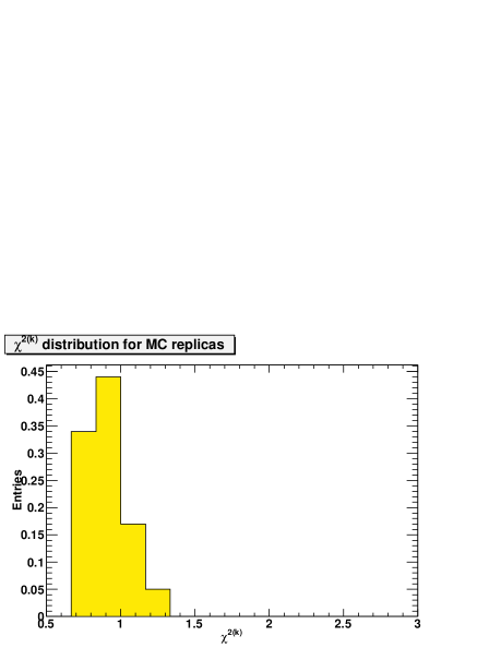
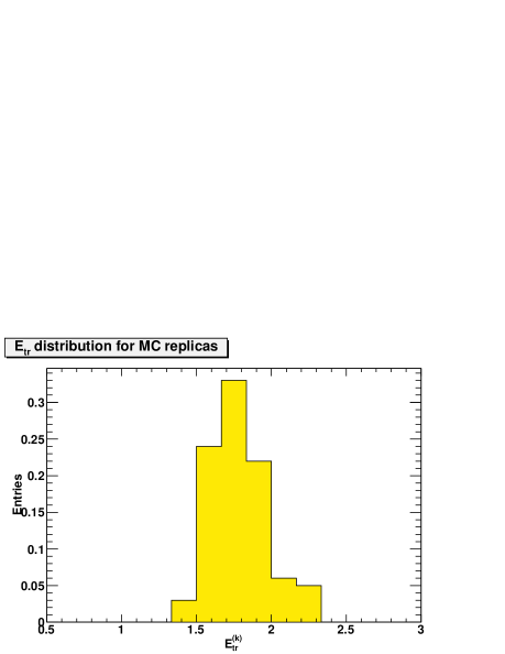
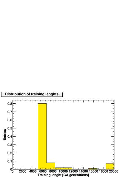
The distribution of $\chi^{2(k)}$, $E_{\mathrm{tr}}^{(k)}$, and training lengths among the $N_{\mathrm{rep}}=100$ replicas are shown in Fig. 4 and Fig. 5 respectively. Note that the latter has a long tail which causes an accumulation of points at the maximum training length, $N_{\mathrm{gen}}^{\mathrm{max}}$. This means that there is a fraction of replicas that do not fulfill the stopping criterion. This may cause a loss in accuracy in outlier fits, which however make up fewer than $10\%$ of the total sample.

The features of the fit can be summarized as follows:

• The quality of the central fit, as measured by its $\chi_{\mathrm{tot}}^{2}=0.77$, is good. However, this value should be taken with care in view of the fact that uncertainties for all experiments but two are overestimated because the covariance matrix is not available and thus correlations between systematics cannot be properly accounted for. This explains the value lower than one for this quantity, which would be very unlikely if it had included correlations.

• The values of $\chi_{\mathrm{tot}}^{2}$ and $\left\langle E\right\rangle$ differ by approximately one unit. This is due to the fact that replicas fluctuate within their uncertainty about the experimental data, which in turn are gaussianly distributed about a true value [49]: it shows that the neural net is correctly reproducing the underlying law thus being closer to the true value. This is confirmed by the fact that $\left\langle\chi^{2(k)}\right\rangle$ is of order one.

  

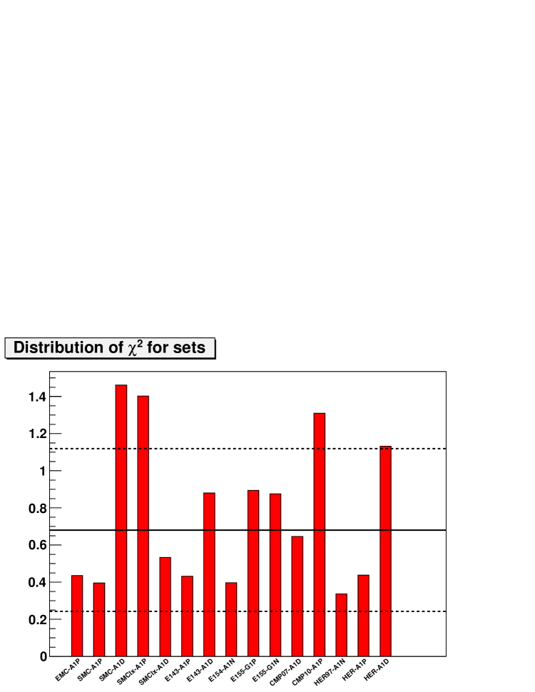
  Figure 6: Value of the $\chi^{2}$ per data point for the datasets included in the NNPDFpol1.0 reference fit, listed in Tab. 10. The horizontal line is the unweighted average of these $\chi^{2}$ over the datasets and the black dashed lines give the one-sigma interval about it.

• The distribution of $\chi^{2}$ for different experiments (also shown as a histogram in Fig. 6) shows sizable differences, and indeed the standard deviation (shown as a dashed line in the plot) about the mean (shown as a solid line) is very large. This can be understood as a consequence of the lack of information on the covariance matrix: experiments where large correlated uncertainties are treated as uncorrelated will necessarily have a smaller value of the $\chi^{2}$.

5.2 Parton distributions

The NNPDFpol1.0 parton distributions, computed from a set of $N_{\mbox{\scriptsize{rep}}}=100$ replicas, are displayed in Fig. 7 at the input scale $Q_{0}^{2}=1$ GeV², in the PDF parametrization basis Eq. (4.1) as a function of $x$ both on a logarithmic and linear scale. In Figs. 8-9 the same PDFs are plotted in the flavour basis, and compared to other available NLO PDF sets: BB10 [11] and AAC08 [12] in Fig. 8, and DSSV08 [15] in Fig. 9. We do not show a direct comparison to the LSS polarized PDFs [14] because there are no publicly available routines for the computation of PDF uncertainties for this set. Note that the dataset used for the BB10 determination contains purely DIS data, and that for AAC contains DIS supplemented by some high-$p_{T}$ RHIC pion production data: hence they are directly comparable to our PDF determination. The DSSV08 determination instead includes, on top of DIS data, polarized jet production data, and, more importantly, a large amount of semi-inclusive DIS data which in particular allow for flavour-antiflavour separation and a more direct handle on strangeness. All uncertainties in these plots correspond to the nominal 1–$\sigma$ error bands.

Figure 7: The NNPDFpol1.0 polarized parton distributions at $Q_{0}^{2}=1$ GeV² in the parametrization basis plotted as a function of $x$, on a logarithmic (left) and linear (right) scale.

Figure 8: Comparison of the NNPDFpol1.0 PDFs (in the flavour basis) and the BB10 [11] and AAC08 [12] PDFs.

Figure 9: Comparison of the NNPDFpol1.0 PDFs (in the flavour basis) and the DSSV08 PDFs [15].

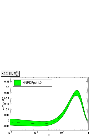
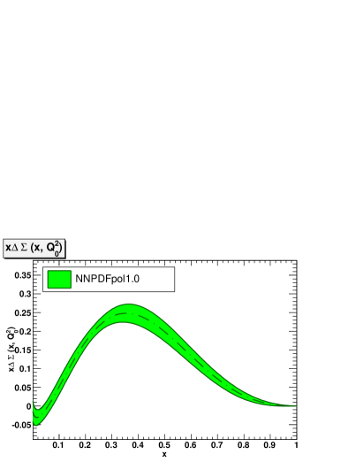
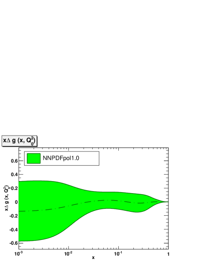
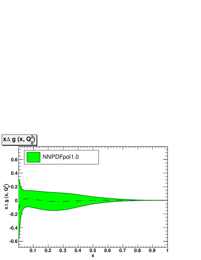
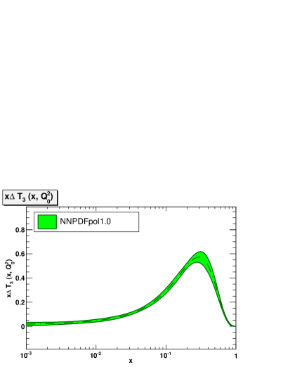
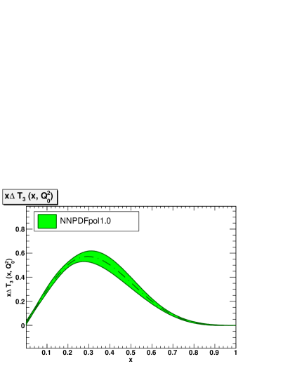
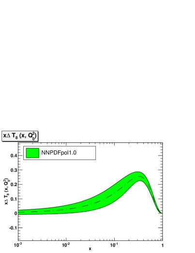
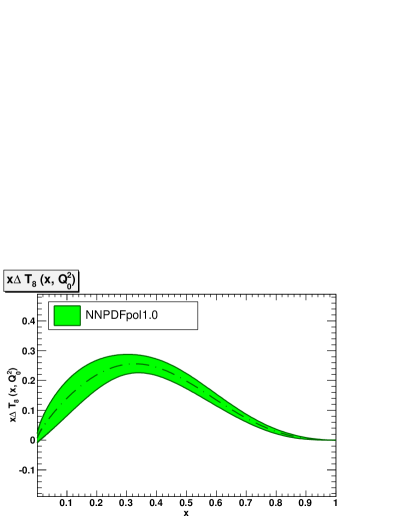
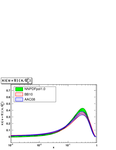
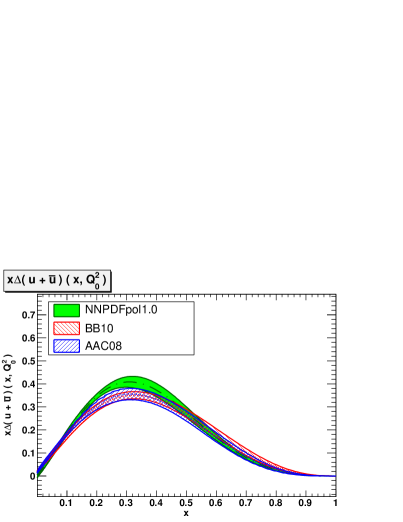
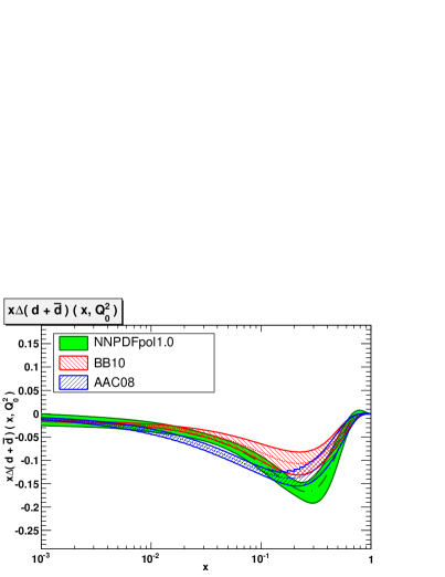
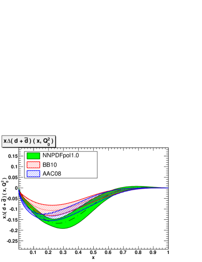
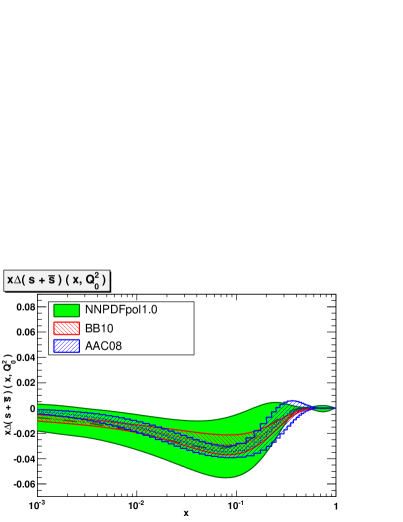
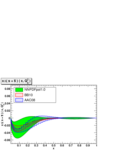
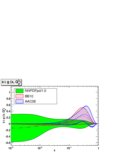
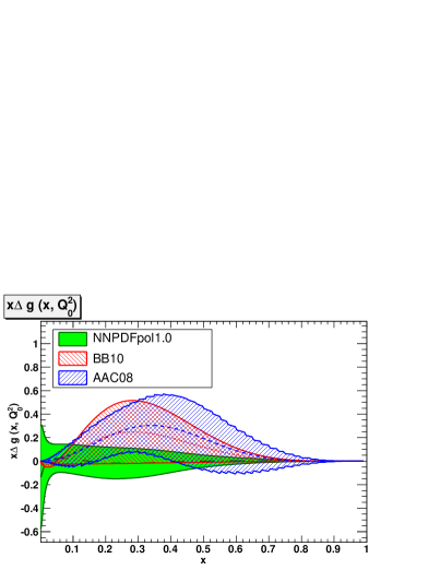
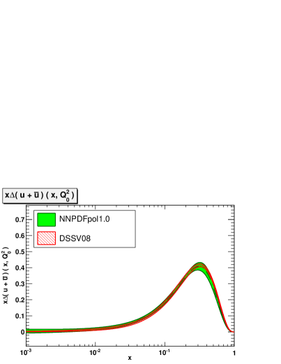
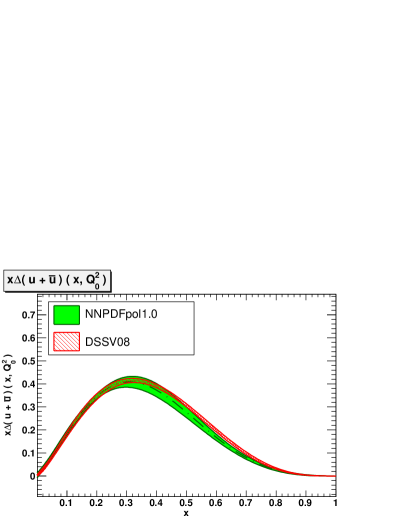
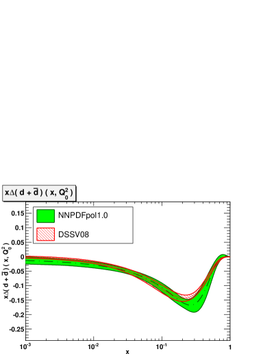
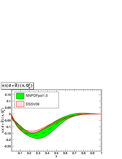
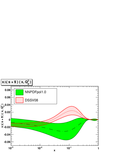
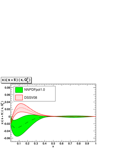
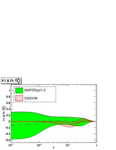
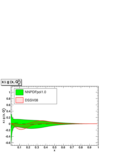
The main conclusions of this comparison are the following:

• The central values of the $\Delta u+\Delta\bar{u}$ and the $\Delta d+\Delta\bar{d}$ are in reasonable agreement with those of other parton sets. The NNPDFpol1.0 results are in best agreement with DSSV08, in slightly worse agreement with AAC08, and in worst agreement with BB10. Uncertainties on these PDFs are generally slightly larger for NNPDF than for other sets, especially DSSV, which however is based on a much wider dataset.

• The NNPDFpol1.0 determination of $\Delta s+\Delta\bar{s}$ is affected by a much larger uncertainty than BB10 and AAC08, for almost all values of $x$. The AAC08 and BB10 strange PDFs fall well within the NNPDFpol1.0 uncertainty band.

• The NNPDFpol1.0 determination of $\Delta s+\Delta\bar{s}$ is inconsistent at the two sigma level in the medium-small $x\sim 0.1$ region with DSSV08, which is also rather more accurate, as one would expect as it includes semi-inclusive data (in particular for production of hadrons with strangeness). This suggests a tension between the inclusive analysis data and the semi-inclusive analysis.

• The gluon PDF is affected by a large uncertainty, rather larger than any other set, especially at small $x$. In particular, the NNPDFpol1.0 polarized gluon distribution is compatible with zero for all values of $x$.

• Uncertainties on the PDFs in the regions where no data are available tend to be larger than those of other sets. At very large values of $x$ the PDF uncertainty band is largely determined by the positivity constraint.

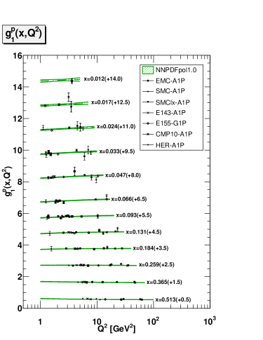
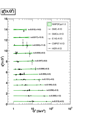
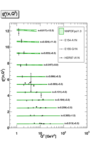
Finally, in Fig. 10 we compare the structure function $g_{1}(x,Q^{2})$ for proton, deuteron and neutron, computed using NNPDFpol1.0 (with its one-$\sigma$ uncertainty band) to the experimental data included in the fit. Experimental data are grouped in bins of $x$ with a logarithmic spacing, while the NNPDF prediction and its uncertainty are computed at the central value of each bin.

The uncertainty band in the NNPDFpol1.0 result is typically smaller than the experimental errors, except at small-$x$ where a much more restricted dataset is available; in that region, the uncertainties are comparable. Scaling violations of the polarized structure functions are clearly visible, especially for $g_{1}^{p}$, despite the limited range in $Q^{2}$.

Figure 10: The proton, neutron and deuteron polarized structure function $g_{1}(x,Q^{2})$ as functions of $Q^{2}$ in different bins of $x$ compared to experimental data. Experimental data are grouped in bins of $x$, while NNPDFpol1.0 results are given at the center of each bin, whose value is given next to each curve. In order to improve legibility, the values of $g_{1}(x,Q^{2})$ have been shifted by the amount given next to each curve.

5.3 Stability of the results

Our results have been obtained with a number of theoretical and methodological assumptions, discussed in Sects. 3-4. We will now test their upon variation of these assumptions.

5.3.1 Target-mass corrections and $g_{2}$.

We have consistently included in our determination of $g_{1}$ corrections suppressed by powers of the nucleon mass which are of kinematic origin. Thus in particular, as explained in Sec. 3.2, we have included target-mass corrections (TMCs) up to first order in ${m^{2}}/{Q^{2}}$. Furthermore, both TMCs and the relation between the measured asymmetries and the structure function $g_{1}$ involve contributions to the structure function $g_{2}$ proportional to powers of ${m^{2}}/{Q^{2}}$ which we include according to Eq. (17) or Eq. (18) (see the discussion in Sect. 2.2). Our default PDF set is obtained assuming that $g_{2}$ is given by the Wandzura-Wilczek relation, Eq. (22).

In order to assess the impact of these assumptions on our results, we have performed two more PDF determinations. In the first, we set $m=0$ consistently everywhere, both in the extraction of the structure functions from the asymmetry data and in our computation of structure functions. This thus removes TMCs, and also contributions proportional to $g_{2}$. In the second, we retain mass effects, but we assume $g_{2}=0$.

The statistical estimators for each of these three fits over the full dataset are shown in Tab. 11. Clearly, all fits are of comparable quality.

Fit	NNPDFpol1.0 $g_{2}=g_{2}^{\mbox{\tiny WW}}$	NNPDFpol1.0 $m=0$	NNPDFpol1.0 $g_{2}=0$
$\chi^{2}_{\rm tot}$	0.77	0.78	0.75
$\left\langle E\right\rangle\pm\sigma_{E}$	1.82 $\pm$ 0.18	1.81 $\pm$ 0.16	1.83 $\pm$ 0.15
$\left\langle E_{\rm tr}\right\rangle\pm\sigma_{E_{\rm tr}}$	1.66 $\pm$ 0.49	1.62 $\pm$ 0.50	1.70 $\pm$ 0.38
$\left\langle E_{\rm val}\right\rangle\pm\sigma_{E_{\rm val}}$	1.88 $\pm$ 0.67	1.84 $\pm$ 0.70	1.96 $\pm$ 0.56
$\left\langle\chi^{2(k)}\right\rangle\pm\sigma_{\chi^{2}}$	0.91 $\pm$ 0.12	0.90 $\pm$ 0.09	0.86 $\pm$ 0.09

Table 11: The statistical estimators of Tab. 9 (obtained assuming $g_{2}=g_{2}^{\mbox{\tiny WW}}$) compared to a fit with $m=0$ or with $g_{2}=0$.

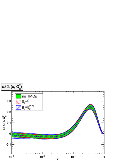
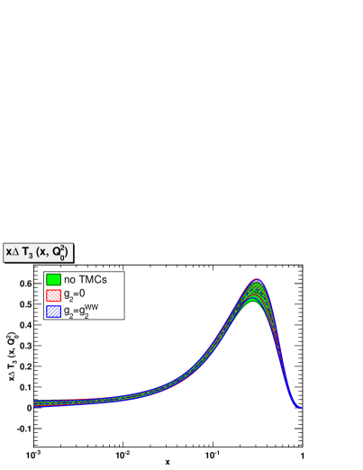
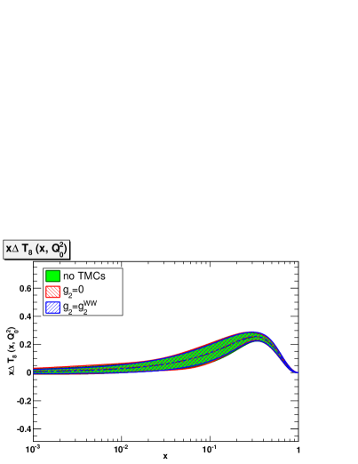
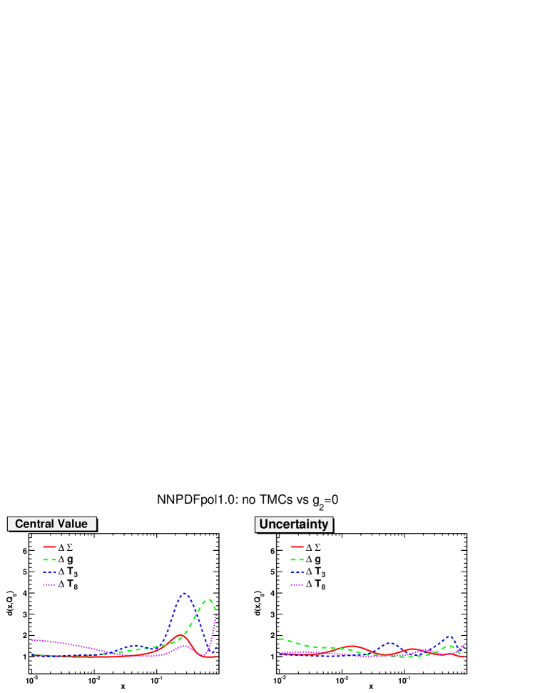
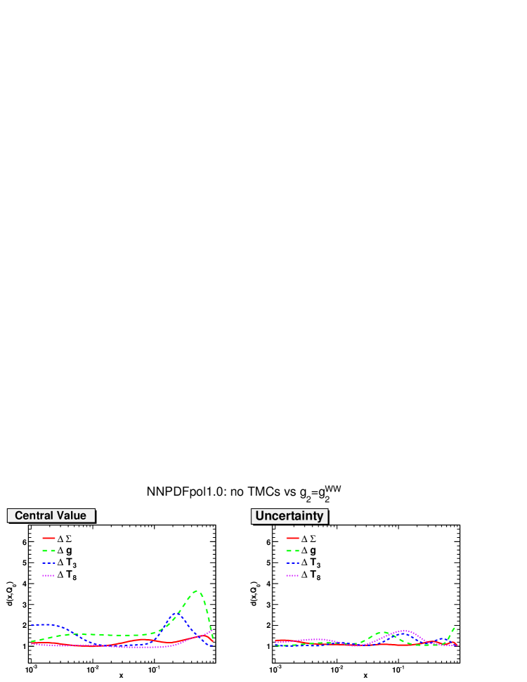
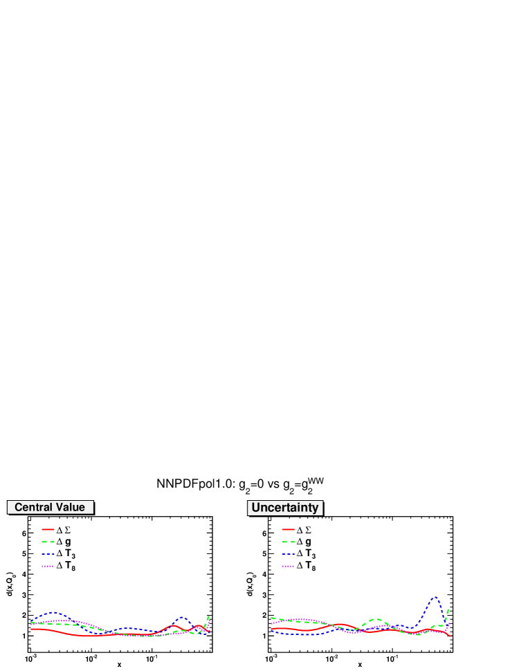
Furthermore, in Fig. 11 we compare the PDFs at the initial scale $Q_{0}^{2}$ determined in these fits to our default set: differences are hardly visible. This comparison can be made more quantitative by using the distance $d(x,Q^{2})$ between different fits, as defined in Appendix A of Ref. [23]. The distance is defined in such a way that if we compare two different samples of $N_{\rm rep}$ replicas each extracted from the same distribution, then on average $d=1$, while if the two samples are extracted from two distributions which differ by one standard deviation, then on average $d=\sqrt{N_{\rm rep}}$ (the difference being due to the fact that the standard deviation of the mean scales as $1/\sqrt{N_{\rm rep}}$).

The distances $d(x,Q^{2})$ between central values and uncertainties of the three fits of Tab. 11 are shown in Fig. 12. They never exceed $d=4$, which means less than half a standard deviation for $N_{\rm rep}=100$. It is interesting to observe that distances tend to be larger in the large-$x$ region, where the expansion in powers of $m^{2}/Q^{2}$ is less accurate, and the effects of dynamical higher twists can become relevant. It is reassuring that even in this region the distances are reasonably small.

We conclude that inclusive DIS data, with our kinematic cuts, do not show sensitivity to finite nucleon mass effects, neither in terms of fit quality, nor in terms of the effect on PDFs.

Figure 11: Comparison between the default NNPDFpol1.0 PDFs (labeled as $g_{2}=g_{2}^{\mbox{\tiny WW}}$ in the plot), PDFs with $m=0$ (labeled as noTMCs in the plot) and PDFs with $g_{2}=0$; each corresponds to the statistical estimators of Tab. 11.

Figure 12: Distances between each pair of the three sets of PDFs shown in Fig. 11.

5.3.2 Sum rules

Our default PDF fit is obtained by assuming that the triplet axial charge $a_{3}$ is fixed to its value extracted from $\beta$ decay, Eq. (37), and that the octet axial charge $a_{8}$ is fixed to the value of $a_{8}$ determined from baryon octet decays, but with an inflated uncertainty in order to allow for SU(3) violation, Eq. (39). As discussed after Eq. (51) uncertainties on them are included by randomizing their values among replicas.

In order to test the impact of these assumptions, we have produced two more PDF determinations. In the first, we have not imposed the triplet sum rule Eq. (35), so in particular $a_{3}$ is free and determined by the data, instead of being fixed to the value Eq. (37). In the second, we have assumed that the uncertainty on $a_{8}$ is given by the much smaller value of Eq. (38).

Fit	free $a_{3}$	$a_{8}$ Eq. (38)
$\chi^{2}_{\rm tot}$	0.79	0.77
$\left\langle E\right\rangle\pm\sigma_{E}$	1.84 $\pm$ 0.19	1.86 $\pm$ 0.19
$\left\langle E_{\rm tr}\right\rangle\pm\sigma_{E_{\rm tr}}$	1.73 $\pm$ 0.41	1.66 $\pm$ 0.53
$\left\langle E_{\rm val}\right\rangle\pm\sigma_{E_{\rm val}}$	1.93 $\pm$ 0.58	1.87 $\pm$ 0.71
$\left\langle\chi^{2(k)}\right\rangle\pm\sigma_{\chi^{2}}$	0.93 $\pm$ 0.12	0.92 $\pm$ 0.15

Table 12: The statistical estimators of Tab. 9, but for fits in which the triplet sum rule is not imposed (free $a_{3}$) or in which the octet sum rule is imposed with the smaller uncertainty Eq. (38).

The statistical estimators for the total dataset for each of these fits are shown in Tab. 12. Here too, there is no significant difference in fit quality between these fits and the default.

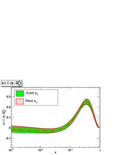
The distances between PDFs in the default and the free $a_{3}$ fits are displayed in Fig. 13. As one may expect, only the triplet is affected significantly: the central value is shifted by about $d\sim 5$, i.e. about half-$\sigma$, in the region $x\sim 0.3$, where $x\Delta T_{3}$ has a maximum, and also around $x\sim 0.01$. The uncertainties on the PDFs are very similar in both cases for all PDFs, except $\Delta T_{3}$ at small-$x$: in this case, removing the $a_{3}$ sum rule results in a moderate increase of the uncertainties; the effect of removing $a_{3}$ is otherwise negligible. The singlet and triplet PDFs for these two fits are compared in Fig. 14.

Figure 13: Distances between PDFs (central values and uncertainties) for the default fit, with $a_{3}$ fixed, and the fit with free $a_{3}$, computed using $N_{\mbox{\tiny rep}}=100$ replicas from each set.

Figure 14: Comparison of the singlet and triplet PDFs for the default fit, with $a_{3}$ fixed, and the fit with free $a_{3}$.

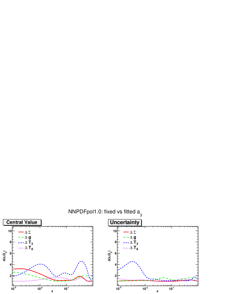
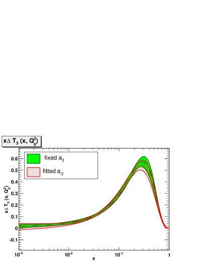
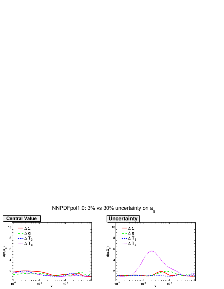
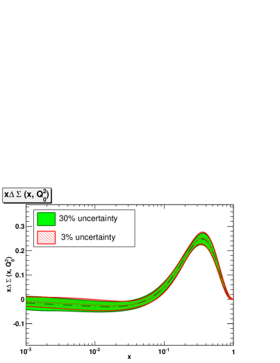
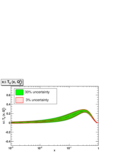
The distances between the default and the fit with the smaller uncertainty on $a_{8}$, Eq. (38), are shown in Fig. 15. In this case, again as expected, the only effect is on the $\Delta T_{8}$ uncertainty, which changes in the region $10^{-2}\lesssim x\lesssim 10^{-1}$ by up to $d\sim 6$ (about half a standard deviation): if a more accurate value of $a_{8}$ is assumed, the determined $\Delta T_{8}$ is correspondingly more accurate. Central values are unaffected. The singlet and octet PDFs for this fit are compared to the default in Fig. 16. We conclude that the size of the uncertainty on $\Delta T_{8}$ has a moderate effect on our fit; on the other hand it is clear that if the octet sum rule were not imposed at all, the uncertainty on the octet and thus on strangeness would increase very significantly, as we have checked explicitly.

Figure 15: Distances between PDFs (central values and uncertainties) for the default fit, with $a_{8}$ Eq. (39), and the fit with the value of $a_{8}$ with smaller uncertainty, Eq. (38).

Figure 16: Comparison of the singlet and octet PDFs for the default fit, with $a_{8}$ Eq. (39), and the fit with the value of $a_{8}$ with smaller uncertainty, Eq. (38).

We conclude that our fit results are quite stable upon variations of our treatment of both the triplet and the octet sum rules.

5.4 Positivity

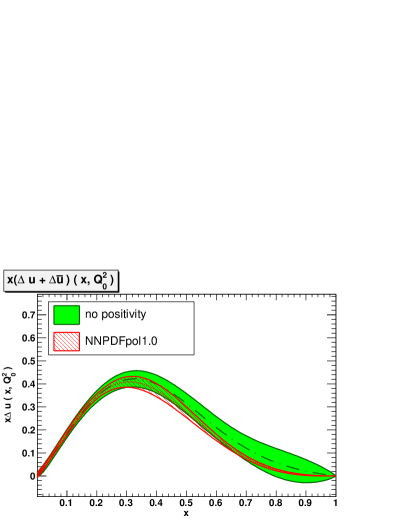
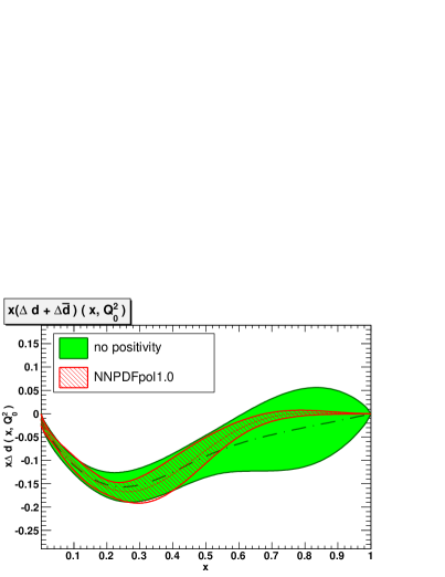
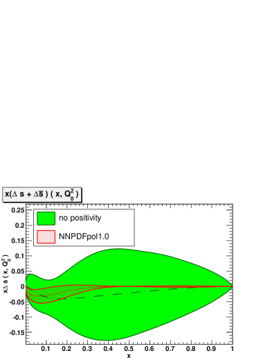
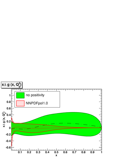
As discussed in Sect. 4, positivity of the individual cross sections entering the polarized asymmetries Eq. (1) has been imposed at leading order according to Eq. (61), using the NNPDF2.1 NNLO PDF set [25], separately for the lightest polarized quark PDF combinations $\Delta u+\Delta\bar{u}$, $\Delta d+\Delta\bar{d}$, $\Delta s+\Delta\bar{s}$ and for the polarized gluon PDF, by means of a Lagrange multiplier Eq. (4.4). After stopping, positivity is checked a posteriori and replicas which do not satisfy it are discarded and retrained.

In Fig. 17 we compare to the positivity bound for the up, down, strange PDF combinations and gluon PDF a set of $N_{\mbox{\tiny rep}}=100$ replicas obtained by enforcing positivity through a Lagrange multiplier, but before the final, a posteriori check. Almost all replicas satisfy the constraint, but at least one replica which clearly violates it for the $s+\bar{s}$ combination (and thus will be discarded) is seen.

Figure 17: The positivity bound Eq. (61), compared to a set of $N_{\mbox{\tiny rep}}=100$ replicas (dashed lines).

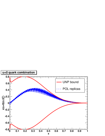
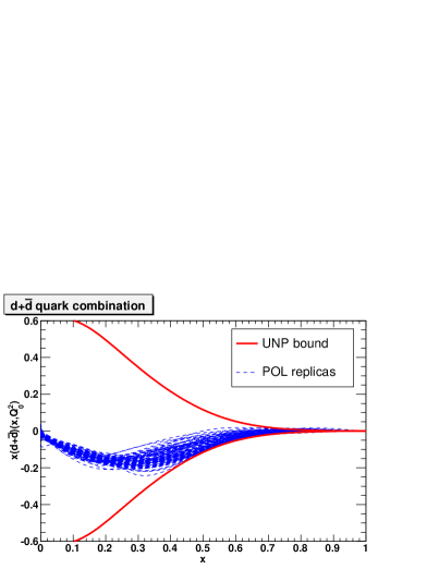
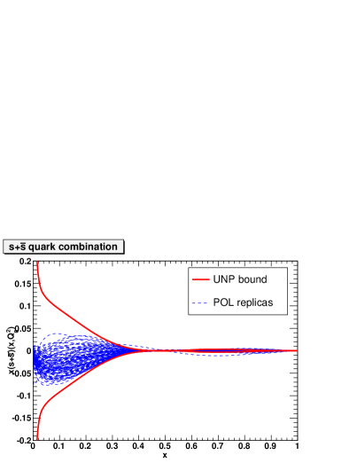
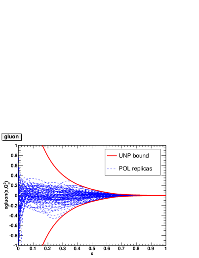
In order to assess the effect of the positivity constraints we have performed a fit without imposing positivity. Because positivity significantly affects PDFs in the region where no data are available, and thus in particular their large $x$ behaviour, preprocessing exponents for this PDF determination had to be determined again using the procedure described in Sect. 4.1. The values of the large $x$ preprocessing exponents used in the fit without positivity are shown in Tab. 13. The small $x$ exponents are the same as in the baseline fit, Tab. 5.

PDF	$m$
$\Delta\Sigma(x,Q_{0}^{2})$	$\left[0.5,5.0\right]$
$\Delta g(x,Q_{0}^{2})$	$\left[0.5,5.0\right]$
$\Delta T_{3}(x,Q_{0}^{2})$	$\left[0.5,4.0\right]$
$\Delta T_{8}(x,Q_{0}^{2})$	$\left[0.5,6.0\right]$

Table 13: Ranges for the large $x$ preprocessing exponents Eq. (4.1) for the fit in which no positivity is imposed. The small $x$ exponents are the same as in the baseline fit Tab. 5.

The corresponding estimators are shown in Tab. 14. Also in this case, we see no significant change in fit quality, with only a slight improvement in $\chi^{2}_{\rm tot}$ when the constraint is removed. This shows that our PDF parametrization is flexible enough to easily accommodate positivity. On the other hand, clearly the positivity bound has a significant impact on PDFs, especially in the large $x$ region, as shown in Fig. 18, where PDFs obtained from this fit are compared to the baseline. At small $x$, instead, the impact of positivity is moderate, because, as discussed in Sect. 4.4, $g_{1}/F_{1}\sim x$ as $x\to 0$ [64] so there is no constraint in the limit. This in particular implies that there is no significant loss of accuracy in imposing the LO positivity bound, because in the small $x\lesssim 10^{-2}$ region, where the LO and NLO positivity bounds differ significantly [65] the bound is not significant.

Fit	NNPDFpol1.0 no positivity
$\chi^{2}_{\rm tot}$	0.72
$\left\langle E\right\rangle\pm\sigma_{E}$	1.84 $\pm$ 0.22
$\left\langle E_{\rm tr}\right\rangle\pm\sigma_{E_{\rm tr}}$	1.60 $\pm$ 0.20
$\left\langle E_{\rm val}\right\rangle\pm\sigma_{E_{\rm val}}$	2.07 $\pm$ 0.39
$\left\langle\chi^{2(k)}\right\rangle\pm\sigma_{\chi^{2}}$	0.95 $\pm$ 0.16

Table 14: The statistical estimators of Tab. 9 for a fit without positivity constraints.

Figure 18: The NNPDFpol1.0 PDFs with and without positivity constraints compared at the initial parametrization scale $Q_{0}^{2}=1$ GeV² in the flavor basis.

5.5 Small- and large-$x$ behaviour and preprocessing

The asymptotic behavior of both polarized and unpolarized PDFs for $x$ close to 0 or 1 is not controlled by perturbation theory, because powers of $\ln\frac{1}{x}$ and $\ln(1-x)$ respectively appear in the perturbative coefficients, thereby spoiling the reliability of the perturbative expansion close to the endpoints. Non-perturbative effects are also expected to set in eventually (see e.g. [67, 64]). For this reason, our fitting procedure makes no assumptions on the large- and small-$x$ behaviors of PDFs, apart from the positivity and integrability constraints discussed in the previous Section.

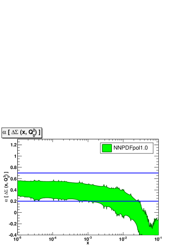
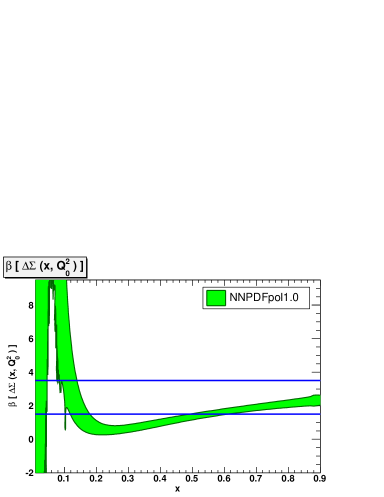
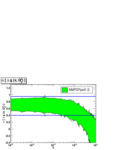
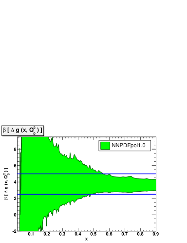
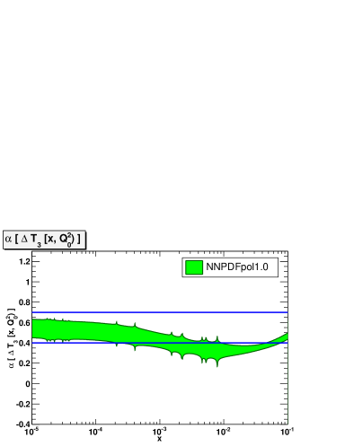
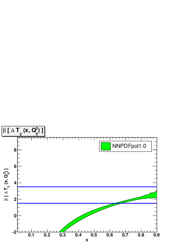
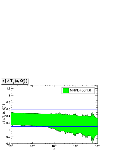
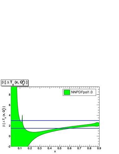
It is however necessary to check that no bias is introduced by the preprocessing. We do this following the iterative method described in Sect. 4.1. The outcome of the procedure is the set of exponents Eq. (4.1), listed in Tab. 5. The lack of bias with these choices is explicitly demonstrated in Fig. 19, where we plot the 68% confidence level of the distribution of

$$\alpha[\Delta q(x,Q^{2})]=\frac{\ln\Delta q(x,Q^{2})}{\ln\frac{1}{x}}\mbox{ ,}$$ (67)

$$\beta[\Delta q(x,Q^{2})]=\frac{\ln\Delta q(x,Q^{2})}{\ln(1-x)}\mbox{ ,}$$ (68)

$\Delta q=\Delta\Sigma\mbox{, }\Delta g\mbox{, }\Delta T_{3}\mbox{, }\Delta T_{8}$, for the default NNPDFpol1.0 $N_{\rm rep}=100$ replica set, at $Q^{2}=Q_{0}^{2}=1$ GeV², and compare them to the ranges of Tab. 5. It is apparent that as the endpoints $x=0$ and $x=1$ are approached, the uncertainties on both the small-$x$ and the large-$x$ exponents lie well within the range of the preprocessing exponents for all PDFs, thus confirming that the latter do not introduce any bias.

Figure 19: The 68% confidence level of the distribution of effective small- and large-$x$ exponents Eqs. (67-68) for the default $N_{\rm rep}=100$ replica NNPDFpol1.0 set at $Q_{0}^{2}=1$ GeV², plotted as functions of $x$. The range of variation of the preprocessing exponents of Tab. 5 is also shown in each case (solid lines).

6 Polarized nucleon structure

The NNPDFpol1.0 PDF set may be used for a determination of the first moments of polarized parton distributions. As briefly summarized in the introduction, these are the quantities of greatest physical interest in that they are directly related to the spin structure of the nucleon, and indeed their determination, in particular the determination of the first moments of the quark and gluon distributions, has been the main motivation for the experimental campaign of $g_{1}$ measurements. The determination of the isotriplet first moment, because of the Bjorken sum rule, provides a potentially accurate and unbiased handle on the strong coupling $\alpha_{s}$.

6.1 First moments

We have computed the first moments

$$\langle\Delta f(Q^{2})\rangle\equiv\int_{0}^{1}dx\,\Delta f(x,Q^{2})$$ (69)

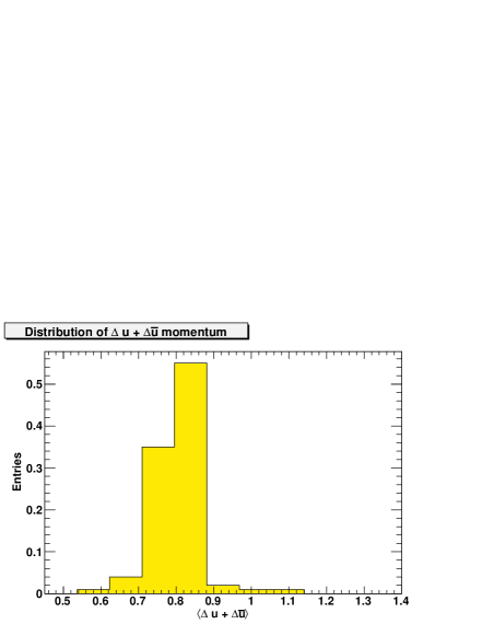
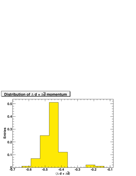
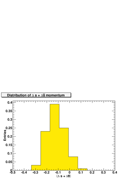
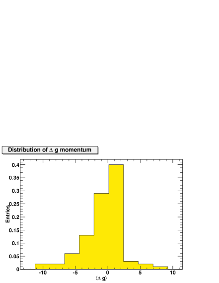
of each light polarized quark-antiquark and gluon distribution using a sample of $N_{\mathrm{rep}}=100$ NNPDFpol1.0 PDF replicas. The histogram of the distribution of first moments over the replica sample at $Q_{0}^{2}=1~{}{\rm GeV^{2}}$ are displayed in Fig. 20: they appear to be reasonably approximated by a Gaussian.

The central value and one-$\sigma$ uncertainties of the quark first moments are listed in Tab. 15, while those of the singlet quark combination Eq. (29) and the gluon are given in Tab. 16. Results are compared to those from other parton sets, namely ABFR98 [8], DSSV10 [15], AAC08 [12], BB10 [11] and LSS10 [14]. Results from other PDF sets are not available for all combinations and scales, because public codes only allow for the computation of first moments in a limited $x$ range, in particular down to a minimum value of $x$: hence we must rely on published values for the first moments. In particular, the DSSV and AAC results are shown at $Q_{0}^{2}=1~{}{\rm GeV^{2}}$, while the BB and LSS results are shown at $Q^{2}=4~{}{\rm GeV^{2}}$. For ease of reference, the NNPDF values for both scales are shown in Tab. 16.

Figure 20: Distribution of the first moments of $\Delta u+\Delta\bar{u}$ (top left), $\Delta d+\Delta\bar{d}$ (top right), $\Delta s+\Delta\bar{s}$ (bottom left) over a set of $N_{\mathrm{rep}}=100$ NNPDFpol1.0 PDF replicas.

	$\langle\Delta u+\Delta\bar{u}\rangle$								$\langle\Delta d+\Delta\bar{d}\rangle$								$\langle\Delta s+\Delta\bar{s}\rangle$
	cv		exp		th		tot		cv		exp		th		tot		cv		exp		th		tot
NNPDFpol1.0	0.	80	0.	08	—		0.	08	-0.	46	0.	08	—		0.	08	-0.	13	0.	09	—		0.	09
DSSV08 [68]	0.	817	0.	013	0.	008	0.	015	-0.	453	0.	011	0.	036	0.	038	-0.	110	0.	023	0.	098	0.	101

Table 15: First moments of the polarized quark distributions at $Q_{0}^{2}=1$ GeV²; cv denotes the central value, whil exp and th denote uncertainties (see text) whose sum in quadrature is given by tot.

In order to compare the results for first moments shown in Tabs. 15-16, it should be understood that the uncertainties shown, and sometimes also the central values, have somewhat different meanings. In particular:

• For NNPDFpol1.0 the exp uncertainty, determined as the standard deviation of the replica sample, is a pure PDF uncertainty: it includes the propagation of the experimental data uncertainties and the uncertainty due to the interpolation and extrapolation.

• In the ABFR98 study, the central values were obtained in the so-called AB factorization scheme [6]. While the gluon in this scheme coincides with the gluon in the $\overline{\rm MS}$ scheme used here (and thus the value from Ref. [8] for the gluon is shown in Tab. 16), the quark singlet differs from it. However, in Ref. [8] a value of the singlet axial charge $a_{0}$ in the limit of infinite $Q^{2}$ was also given. In the $\overline{\rm MS}$, the singlet axial charge and the first moment of $\Delta\Sigma$ coincide [6], hence we have determined $\left\langle\Delta\Sigma\right\rangle$ for ABFR98 by evolving down to $Q^{2}=1$ GeV² the value of $a_{0}(\infty)$ given in Ref. [8], at NLO and with $\alpha_{s}(M_{z})=0.118$ [69] (the impact of the $\alpha_{s}$ uncertainty is negligible). We have checked that the same result is obtained if $a_{0}$ is computed as the appropriate linear combination of $\left\langle\Delta\Sigma\right\rangle$ in the AB scheme and the first moment of $\Delta g$. In the ABFR98 study, the exp uncertainty is the Hessian uncertainty on the best fit, and it thus includes the propagated data uncertainty. The th uncertainty includes the uncertainty originated by neglected higher orders (estimated by renormalization and factorization scale variations), higher twists, position of heavy quark thresholds, value of the strong coupling, violation of SU(3) (uncertainty on $a_{8}$ Eq. (36)), and finally uncertainties related to the choice of functional form, estimated by varying the functional form. This latter source of theoretical uncertainty corresponds to interpolation and extrapolation uncertainties which are included in the exp for NNPDF.

• For DSSV08 and BB10 PDFs, the central value is obtained by computing the first moment integral of the best-fit with a fixed functional form restricted to the data region, and then supplementing it with a contribution due to the extrapolation in the unmeasured (small $x$) region. The exp uncertainty in the table is the Hessian uncertainty given by DSSV08 or BB10 on the moment in the measured region, and it thus includes the propagated data uncertainty. In both cases, we have determined the th uncertainty shown in the table as the difference between the full first moment quoted by DSSV08 or BB10, and the first moment in the measured region. It is thus the contribution from the extrapolation region, which we assume to be $100\%$ uncertain. In both cases, we have computed the truncated first moment in the measured region using publicly available codes, and checked that it coincides with the values quoted by DSSV08 and BB10.

• For AAC08, the central value is obtained by computing the first moment integral of the best-fit with a fixed functional form, and the exp uncertainty is the Hessian uncertainty on it. However, AAC08 uses a so-called tolerance [70] criterion for the determination of Hessian uncertainties, which rescales the $\Delta\chi^{2}=1$ region by a suitable factor, in order to effectively keep into account also interpolation errors. Hence, the exp uncertainties include propagated data uncertainties, as well as uncertainties on the PDF shape.

• For LSS10, the central value is obtained by computing the first moment integral of the best-fit with a fixed functional form, and the exp uncertainty is the Hessian uncertainty on it. Hence it includes the propagated data uncertainty.

		$\langle\Delta\Sigma\rangle$								$\langle\Delta g\rangle$
		cv		exp		th		tot		cv		exp		th		tot
NNPDFpol1.0 (1GeV2)		0.	22	0.	20	—		0.	20	-1.	2	4.	2	—		4.	2
NNPDFpol1.0 (4GeV2)		0.	18	0.	20	—		0.	20	-0.	9	3.	9	—		4.	2
ABFR98 [8]		0.	12	0.	05	${}^{+0.19}_{-0.12}$		${}^{+0.19}_{-0.13}$		1.	6	0.	4	0.	8	0.	9
DSSV08 [68]		0.	255	0.	019	0.	126	0.	127	-0.	12	0.	12	0.	06	0.	13
AAC08 [12]	(positive)	0.	26	0.	06	—		0.	06	0.	40	0.	28	—		0.	28
	(node)	0.	25	0.	07	—		0.	07	-0.	12	1.	78	—		1.	78
BB10 [11]		0.	19	0.	08	0.	23	0.	24	0.	46	0.	43	0.	004	0.	43
LSS10 [14]	(positive)	0.	207	0.	034	—		0.	034	0.	316	0.	190	—		0.	190
	(node)	0.	254	0.	042	—		0.	042	-0.	34	0.	46	—		0.	46

Table 16: Same as Tab. 15, but for the total singlet quark distribution and the gluon distribution. The NNPDF results are shown both at $Q_{0}^{2}=1$ GeV² and $Q^{2}=4~{}{\rm GeV^{2}}$, the ABFR, DSSV and AAC results are shown at $Q_{0}^{2}=1$ GeV², and the BB10 and LSS10 are shown at $Q^{2}=4~{}{\rm GeV^{2}}$).

In all cases, the total uncertainty is computed as the sum in quadrature of the exp and th uncertainties. Roughly speaking, for LSS10 this includes only the data uncertainties; for DSSV08, and BB10 it also includes extrapolation uncertainties; for AAC08 interpolation uncertainties; for NNPDFpol1.0 both extrapolation and interpolation uncertainties; and for ABFR98 all of the above, but also theoretical (QCD) uncertainties. For LSS10 and AAC08, we quote the results obtained from two different fits, both assuming positive- or node-gluon PDF: their spread gives a feeling for the missing uncertainty due to the choice of functional form. Note that the AAC08 results correspond to their Set B which includes, besides DIS data, also RHIC $\pi^{0}$ production data; the DSSV08 fit also includes, on top of these, RHIC jet data and semi-inclusive DIS data; LSS10 includes, beside DIS, also semi-inclusive DIS data. All other sets are based on DIS data only.

Coming now to a comparison of results, we see that for the singlet first moment $\langle\Delta\Sigma\rangle$ the NNPDFpol1.0 result is consistent within uncertainties with that of other groups. The uncertainty on the NNPDFpol1.0 result is comparable (if somewhat larger) to that found whenever the extrapolation uncertainty has been included. For individual quark flavors (Tab. 15) we find excellent agreement in the central values obtained between NNPDFpol1.0 and DSSV08; the NNPDF uncertainties are rather larger, but this could also be due to the fact that the DSSV08 dataset is sensitive to flavour separation.

For the gluon first moment $\langle\Delta g\rangle$, the NNPDFpol1.0 result is characterized by an uncertainty which is much larger than that of any other determination: a factor of three or four larger than ABFR98 and AAC08, ten times larger than BB10, and twenty times larger than DSSV08 and LSS10. It is compatible with zero within this large uncertainty. We have seen that for the quark singlet, the NNPDFpol1.0 uncertainty is similar to that of groups which include an estimate of extrapolation uncertainties. In order to assess the impact of the extrapolation uncertainty for the gluon, we have computed the gluon first truncated moment in the region $x\in[10^{-3},1]$:

$$\int_{10^{-3}}^{1}dx\,\Delta g(x,Q^{2}=1~{}{\rm GeV^{2}})=-0.26\pm 1.19\,,$$ (70)

to be compared with the result of Tab. 16, which is larger by almost a factor four.

We must conclude that the experimental status of the gluon first moment is still completely uncertain, unless one is willing to make strong theoretical assumptions on the behaviour of the polarized gluon at small $x$, and that previous different conclusions were affected by a significant under-estimate of the impact of the bias in the choice of functional form, in the data and especially in the extrapolation region. Because of the large uncertainty related to the extrapolation region, only low $x$ data can improve this situation, such as those which could be collected at a high energy electron-ion collider [71, 32].

6.2 The Bjorken sum rule

Perturbative factorization, expressed in this context by Eq. (28) for the structure function $g_{1}(x,Q^{2})$, and the assumption of exact isospin symmetry, immediately lead to the so-called Bjorken sum rule (originally derived [72, 73] using current algebra):

$$\Gamma_{1}^{p}\left(Q^{2}\right)-\Gamma_{1}^{n}\left(Q^{2}\right)=\frac{1}{6}\Delta C_{\mathrm{NS}}(\alpha_{s}(Q^{2}))a_{3}\ ,$$ (71)

where

$$\Gamma_{1}^{p,n}(Q^{2})\equiv\int_{0}^{1}dx\,g_{1}^{p,n}(x,Q^{2})\ ,$$ (72)

and $\Delta C_{\mathrm{NS}}(\alpha_{s}(Q^{2}))$ is the first moment of the non-singlet coefficient function, while $a_{3}$ is defined in Eq. (35).

Because the first moment of the non-singlet coefficient function $\Delta C_{\rm NS}$ is known up to three loops [74] and isospin symmetry is expected to hold to high accuracy, the Bjorken sum rule Eq. (71) potentially provides a theoretically very accurate handle on the strong coupling constant: in principle, the truncated isotriplet first moment

$$\Gamma_{1}^{\rm NS}\left(Q^{2},x_{\rm min}\right)\equiv\int_{x_{\rm min}}^{1}dx\left[g_{1}^{p}\left(x,Q^{2}\right)-g_{1}^{n}\left(x,Q^{2}\right)\right]$$ (73)

can be extracted from the data without any theoretical assumption. Given a measurement of $\Gamma_{1}^{\rm NS}\left(Q^{2},0\right)$ at one scale the strong coupling can then be extracted from Eq. (71) using the value of $a_{3}$ from $\beta$ decays, while given a measurement of $\Gamma_{1}^{\rm NS}\left(Q^{2},0\right)$ at two scales both $a_{3}$ and the value of $\alpha_{s}$ can be extracted simultaneously.

In Ref. [75], $a_{3}$ and $\alpha_{s}$ where simultaneously determined from a set of nonsinglet truncated moments (both the first and higher moments), by exploiting the scale dependence of the latter [76], with the result $g_{A}=1.04\pm 0.13$ and $\alpha_{s}(M_{z})=0.126^{+0.006}_{-0.014}$, where the uncertainty is dominated by the data, interpolation and extrapolation, but also includes theoretical (QCD) uncertainties. In this reference, truncated moments were determined from a neural network interpolation of existing data, sufficient for a computation of moments at any scale. However, because the small $x$ behaviour of the structure function is only weakly constrained by data, the $x\to 0$ extrapolation was done by assuming a powerlike (Regge) behaviour [77].

Figure 21: The truncated Bjorken sum rule $\Gamma_{1}^{\rm NS}\left(Q^{2},x\right)$ Eq. (73) plotted as a function of $x$ for $Q^{2}=1$ GeV², for the fit with free $a_{3}$ (left) and for the reference fit with $a_{3}$ fixed to the value Eq. (37), (right panel). In the left plot, the shaded band corresponds to the asymptotic value of the truncated sum rule, Eq. (75), while in the right plot it corresponds to the experimental value Eq. (37).

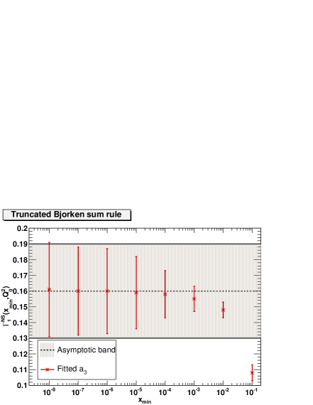
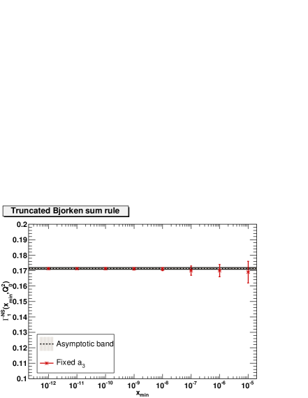
The situation within NNPDFpol1.0 can be understood by exploiting the PDF determination in which $a_{3}$ is not fixed by the triplet sum rule, discussed in Sect. 5.3.2. Using the results of this determination, we find

$$a_{3}=\int_{0}^{1}dx\,\Delta T_{3}(x,Q^{2})=1.19\pm 0.22\ .$$ (74)

The uncertainty is about twice that of the determination of Ref. [75]. As mentioned, the latter was obtained from a neural network parametrization of the data with no theoretical assumptions, and based on a methodology which is quite close to that of the NNPDFpol1.0 PDF determination discussed here, the only difference being the assumption of Regge behaviour in order to perform the small $x$ extrapolation. This strongly suggests that, as in the case of the gluon distribution discussed above, the uncertainty on the value Eq. (74) is dominated by the small $x$ extrapolation.

To study this, in Fig. 21 we plot the value of the truncated Bjorken sum rule $\Gamma_{1}^{\rm NS}\left(Q^{2},x_{\rm min}\right)$ Eq. (73) as a function of the lower limit of integration $x_{\rm min}$ at $Q_{0}^{2}=1$ GeV², along with the asymptotic value

$$\Gamma_{1}^{\rm NS}\left(1~{}\hbox{GeV}^{2},0\right)=0.16\pm 0.03$$ (75)

which at NLO corresponds to the value of $a_{3}$ given by Eq. (74). As a consistency check, we also show the same plot for our baseline fit, in which $a_{3}$ is fixed by the sum rule to the value Eq. (37). It is clear that indeed the uncertainty is completely dominated by the small $x$ extrapolation.

This suggests that a determination of $\alpha_{s}$ from the Bjorken sum rule is not competitive unless one is willing to make assumptions on the small $x$ behaviour of the nonsinglet structure function in the unmeasured region. Indeed, it is clear that a determination based on NNPDFpol1.0 would be affected by an uncertainty which is necessarily larger than that found in Ref. [75], which is already not competitive. The fact that a determination of $\alpha_{s}$ from the Bjorken sum rule is not competitive due to small $x$ extrapolation ambiguities was already pointed out in Ref. [8], where values of $a_{3}$ and $\alpha_{s}$ similar to those of Ref. [75] were obtained.

7 Conclusions and outlook

We have presented a first determination of polarized parton distributions based on the NNPDF methodology: NNPDFpol1.0. We have determined polarized PDFs from the most recent inclusive data on proton, deuteron and neutron deep-inelastic polarized asymmetries and structure functions. Our main result is that the uncertainty in the gluon distribution, and to a lesser extent the strange distribution, and in the small $x$ extrapolation for all parton distributions, is rather larger than in previous polarized PDF determinations. Also, there seems to be some tension between strangeness determined in deep-inelastic scattering and using sem-inclusive data.

In particular, we find that the role of the gluon distribution in the spin structure of the nucleon is essentially unknown, as the first moment of the gluon distribution is compatible with zero, but with an uncertainty which is compatible with a very large positive or negative gluon spin fraction. Likewise, the contribution from the small $x$ region to the Bjorken sum rule makes its use as a means to determine $\alpha_{s}$ essentially impossible. Different conclusions can be reached only if one is willing to make strong theoretical assumptions on the small $x$ behaviour of polarized PDFs.

Future experiments, in particular open charm and hadron production in fixed target experiments, [87, 78] inclusive jet production [80, 81] and $W$ boson production [82, 83, 84] from the RHIC collider may improve the knowledge on individual polarized flavors and antiflavors and on the gluon distribution in the valence region. However, only a high-energy electron-ion collider [71, 32] might provide information on polarized PDFs at small $x$ and thus reduce the uncertainty on first moments in a significant way.

 

The NNPDFpol1.0 polarized PDFs, with $N_{\rm rep}=100$ replicas, are available from the NNPDF HEPFORGE web site,

http://nnpdf.hepforge.org/ .

A Mathematica driver code is also available from the same source.

Acknowledgments

We would like to thank C. Aidala and G. Altarelli for encouragement in this project, D. De Florian, D. Hasch, A. Bacchetta and M. Radici for useful discussions on polarized PDFs. We thank G. Salam for assistance with the polarized PDF evolution Les Houches benchmark tables. The research of JR has been supported by a Marie Curie Intra–European Fellowship of the European Community’s 7th Framework Programme under contract number PIEF-GA-2010-272515. SF, ERN and GR are supported by a PRIN2010 grant.

Appendix A Benchmarking of polarized PDF evolution

We have benchmarked our implementation of the evolution of polarized parton densities by cross-checking against the Les Houches polarized PDF evolution benchmark tables [85]. Note that in Ref. [85] the polarized sea PDFs are given incorrectly, and should be

$$x\Delta\bar{u}=-0.045x^{0.3}(1-x)^{7}$$

$$x\Delta\bar{d}=-0.055x^{0.3}(1-x)^{7}\ .$$ (76)

These tables were obtained from a comparison of the HOPPET [58] and PEGASUS [86] evolution codes, which are $x-$space and $N-$space codes respectively. In order to perform a meaningful comparison, we use the so-called iterated solution of the $N-$space evolution equations and use the same initial PDFs and running coupling as in [85]. The relative difference $\epsilon_{\rm rel}$ between our PDF evolution and the benchmark tables of Refs. [85] at NLO in the ZM-VFNS scheme are tabulated in Tab. 17 for various combinations of polarized PDFs: the accuracy of our code is $\mathcal{O}\left(10^{-5}\right)$ for all relevant values of $x$, which is the nominal accuracy of the agreement between HOPPET and PEGASUS.

$x$	$\epsilon_{\rm rel}\left(\Delta u_{V}\right)$	$\epsilon_{\rm rel}\left(\Delta d_{V}\right)$	$\epsilon_{\rm rel}\left(\Delta\Sigma\right)$	$\epsilon_{\rm rel}\left(\Delta g\right)$
$10^{-3}$	$1.1\,10^{-4}$	$9.2\,10^{-5}$	$9.9\,10^{-5}$	$1.1\,10^{-4}$
$10^{-2}$	$1.4\,10^{-4}$	$1.9\,10^{-4}$	$3.5\,10^{-4}$	$9.3\,10^{-5}$
$0.1$	$1.2\,10^{-4}$	$1.6\,10^{-4}$	$5.4\,10^{-6}$	$1.7\,10^{-4}$
$0.3$	$2.3\,10^{-6}$	$1.1\,10^{-5}$	$7.5\,10^{-6}$	$1.7\,10^{-5}$
$0.5$	$5.6\,10^{-6}$	$9.6\,10^{-6}$	$1.6\,10^{-5}$	$2.5\,10^{-5}$
$0.7$	$1.2\,10^{-4}$	$9.2\,10^{-7}$	$1.6\,10^{-4}$	$7.8\,10^{-5}$
$0.9$	$3.5\,10^{-3}$	$1.1\,10^{-2}$	$4.1\,10^{-3}$	$7.8\,10^{-3}$

Table 17: Percentage difference between FastKernel perturbative evolution of polarized PDFs and the Les Houches benchmark tables [85] for different polarized PDF combinations at NLO in the ZM-VFNS scheme.

Therefore, we can conclude that the accuracy of the polarized PDF evolution in the FastKernel framework is satisfactory for precision phenomenology.

References

- [1] European Muon Collaboration, J. Ashman et al., Phys.Lett. B206 (1988) 364.
- [2] European Muon, J. Ashman et al., Nucl. Phys. B328 (1989) 1.
- [3] G. Altarelli and G.G. Ross, Phys.Lett. B212 (1988) 391.
- [4] G. Altarelli and B. Lampe, Z.Phys. C47 (1990) 315.
- [5] D. de Florian et al., Prog.Part.Nucl.Phys. 67 (2012) 251, 1112.0904.
- [6] R.D. Ball, S. Forte and G. Ridolfi, Phys. Lett. B378 (1996) 255, hep-ph/9510449.
- [7] G. Altarelli et al., Nucl. Phys. B496 (1997) 337, hep-ph/9701289.
- [8] G. Altarelli et al., Acta Phys. Polon. B29 (1998) 1145, hep-ph/9803237.
- [9] T. Gehrmann and W.J. Stirling, Phys.Rev. D53 (1996) 6100, hep-ph/9512406.
- [10] J. Blumlein and H. Bottcher, Nucl. Phys. B636 (2002) 225, hep-ph/0203155.
- [11] J. Blumlein and H. Bottcher, Nucl.Phys. B841 (2010) 205, 1005.3113.
- [12] Asymmetry Analysis Collaboration, M. Hirai and S. Kumano, Nucl.Phys. B813 (2009) 106, 0808.0413.
- [13] E. Leader, A.V. Sidorov and D.B. Stamenov, Phys. Rev. D75 (2007) 074027, hep-ph/0612360.
- [14] E. Leader, A.V. Sidorov and D.B. Stamenov, Phys.Rev. D82 (2010) 114018, 1010.0574.
- [15] D. de Florian et al., Phys. Rev. D80 (2009) 034030, 0904.3821.
- [16] S. Forte, Acta Phys.Polon. B41 (2010) 2859, 1011.5247.
- [17] S. Forte and G. Watt, (2013), 1301.6754.
- [18] NNPDF Collaboration, L. Del Debbio et al., JHEP 03 (2005) 080, hep-ph/0501067.
- [19] NNPDF Collaboration, L. Del Debbio et al., JHEP 03 (2007) 039, hep-ph/0701127.
- [20] NNPDF Collaboration, R.D. Ball et al., Nucl. Phys. B809 (2009) 1, 0808.1231.
- [21] NNPDF Collaboration, R.D. Ball et al., JHEP 1005 (2010) 075, 0912.2276.
- [22] NNPDF Collaboration, R.D. Ball et al., Nucl. Phys. B823 (2009) 195, 0906.1958.
- [23] NNPDF Collaboration, R.D. Ball et al., Nucl.Phys. B838 (2010) 136, 1002.4407.
- [24] NNPDF Collaboration, R.D. Ball et al., Nucl.Phys. B849 (2011) 112, 1012.0836.
- [25] NNPDF Collaboration, R.D. Ball et al., Nucl.Phys. B849 (2011) 296, 1101.1300.
- [26] NNPDF Collaboration, R.D. Ball et al., Nucl.Phys. B855 (2012) 153, 1107.2652.
- [27] NNPDF Collaboration, R.D. Ball et al., (2011), 1110.1863.
- [28] NNPDF Collaboration, R.D. Ball et al., Nucl.Phys. B855 (2012) 608, 1108.1758.
- [29] NNPDF Collaboration, R.D. Ball et al., Nucl.Phys. B867 (2013) 244, 1207.1303.
- [30] S. Forte, M.L. Mangano and G. Ridolfi, Nucl.Phys. B602 (2001) 585, hep-ph/0101192.
- [31] M.L. Mangano et al., (2001), hep-ph/0105155.
- [32] D. Boer et al., (2011), 1108.1713.
- [33] R.K. Ellis, W.J. Stirling and B. Webber, Camb.Monogr.Part.Phys.Nucl.Phys.Cosmol. 8 (1996) 1.
- [34] E143, K. Abe et al., Phys. Rev. D58 (1998) 112003, hep-ph/9802357.
- [35] E155 Collaboration, P. Anthony et al., Phys.Lett. B553 (2003) 18, hep-ex/0204028.
- [36] A. Airapetian et al., Eur.Phys.J. C72 (2012) 1921, 1112.5584.
- [37] S. Wandzura and F. Wilczek, Phys. Lett. B72 (1977) 195.
- [38] A. Accardi et al., JHEP 0911 (2009) 093, 0907.2942.
- [39] J. Blumlein and H. Bottcher, (2012), 1207.3170.
- [40] V. Braun et al., Phys.Rev. D83 (2011) 094023, 1103.1269.
- [41] Spin Muon Collaboration, B. Adeva et al., Phys.Rev. D58 (1998) 112001.
- [42] Spin Muon Collaboration, B. Adeva et al., Phys.Rev. D60 (1999) 072004.
- [43] E154, K. Abe et al., Phys. Rev. Lett. 79 (1997) 26, hep-ex/9705012.
- [44] E155, P.L. Anthony et al., Phys. Lett. B493 (2000) 19, hep-ph/0007248.
- [45] COMPASS, V.Y. Alexakhin et al., Phys. Lett. B647 (2007) 8, hep-ex/0609038.
- [46] COMPASS, M.G. Alekseev et al., Phys. Lett. B690 (2010) 466, 1001.4654.
- [47] HERMES Collaboration, K. Ackerstaff et al., Phys.Lett. B404 (1997) 383, hep-ex/9703005.
- [48] HERMES, A. Airapetian et al., Phys. Rev. D75 (2007) 012007, hep-ex/0609039.
- [49] S. Forte et al., JHEP 05 (2002) 062, hep-ph/0204232.
- [50] C. Simolo, (2006), 0807.1501.
- [51] Jefferson Lab Hall A, X. Zheng et al., Phys. Rev. C70 (2004) 065207, nucl-ex/0405006.
- [52] CLAS Collaboration, R. Fatemi et al., Phys.Rev.Lett. 91 (2003) 222002, nucl-ex/0306019.
- [53] CLAS, K.V. Dharmawardane et al., Phys. Lett. B641 (2006) 11, nucl-ex/0605028.
- [54] S. Forte et al., Nucl.Phys. B834 (2010) 116, 1001.2312.
- [55] Particle Data Group, K. Nakamura et al., J.Phys.G G37 (2010) 075021.
- [56] R. Flores-Mendieta, E.E. Jenkins and A.V. Manohar, Phys.Rev. D58 (1998) 094028, hep-ph/9805416.
- [57] N. Cabibbo, E.C. Swallow and R. Winston, Ann.Rev.Nucl.Part.Sci. 53 (2003) 39, hep-ph/0307298.
- [58] G.P. Salam and J. Rojo, Comput. Phys. Commun. 180 (2009) 120, 0804.3755.
- [59] Z.J. Ajaltouni et al., (2009), 0903.3861.
- [60] A. Piccione and G. Ridolfi, Nucl. Phys. B513 (1998) 301, hep-ph/9707478.
- [61] J. Rojo and J.I. Latorre, JHEP 01 (2004) 055, hep-ph/0401047.
- [62] C.M. Bishop, Neural Networks for Pattern Recognition (Oxford University Press, 1995).
- [63] G. Altarelli, S. Forte and G. Ridolfi, Nucl. Phys. B534 (1998) 277, hep-ph/9806345.
- [64] R.D. Ball, S. Forte and G. Ridolfi, Nucl. Phys. B444 (1995) 287, hep-ph/9502340.
- [65] S. Forte, G. Altarelli and G. Ridolfi, Nucl.Phys.Proc.Suppl. 74 (1999) 138, hep-ph/9808462.
- [66] S. Alekhin et al., (2011), 1101.0536.
- [67] R. Roberts, (1990).
- [68] D. de Florian et al., Phys.Rev.Lett. 101 (2008) 072001, 0804.0422.
- [69] Particle Data Group, J. Beringer et al., Phys.Rev. D86 (2012) 010001.
- [70] J. Pumplin et al., JHEP 0207 (2002) 012, hep-ph/0201195.
- [71] A. Deshpande et al., Ann.Rev.Nucl.Part.Sci. 55 (2005) 165, hep-ph/0506148.
- [72] J. Bjorken, Phys.Rev. 148 (1966) 1467.
- [73] J. Bjorken, Phys.Rev. D1 (1970) 1376.
- [74] S.A. Larin and J.A.M. Vermaseren, Phys. Lett. B259 (1991) 345.
- [75] L. Del Debbio, A. Guffanti and A. Piccione, JHEP 0911 (2009) 060, 0907.2506.
- [76] S. Forte and L. Magnea, Phys.Lett. B448 (1999) 295, hep-ph/9812479.
- [77] F. Close and R. Roberts, Phys.Lett. B336 (1994) 257, hep-ph/9407204.
- [78] COMPASS Collaboration, C. Adolph et al., (2012), 1202.4064.
- [79] COMPASS Collaboration, M. Alekseev et al., (2008), 0802.3023.
- [80] PHENIX Collaboration, A. Adare et al., Phys.Rev. D84 (2011) 012006, 1009.4921.
- [81] STAR Collaboration, L. Adamczyk et al., (2012), 1205.2735.
- [82] STAR Collaboration, M.M. Aggarwal et al., (2010), 1009.0326.
- [83] PHENIX Collaboration, A. Adare et al., (2010), 1009.0505.
- [84] STAR Collaboration, J.R. Stevens, (2013), 1302.6639.
- [85] M. Dittmar et al., (2005), hep-ph/0511119.
- [86] A. Vogt et al., Nucl. Phys. Proc. Suppl. 183 (2008) 155, 0807.1238.
- [87] COMPASS Collaboration, C. Adolph et al., (2012), 1211.6849.