Detecting Overlapping Temporal Community Structure in Time-Evolving Networks
Abstract
We present a principled approach for detecting overlapping temporal community structure in dynamic networks. Our method is based on the following framework: find the overlapping temporal community structure that maximizes a quality function associated with each snapshot of the network subject to a temporal smoothness constraint. A novel quality function and a smoothness constraint are proposed to handle overlaps, and a new convex relaxation is used to solve the resulting combinatorial optimization problem. We provide theoretical guarantees as well as experimental results that reveal community structure in real and synthetic networks. Our main insight is that certain structures can be identified only when temporal correlation is considered and when communities are allowed to overlap. In general, discovering such overlapping temporal community structure can enhance our understanding of real-world complex networks by revealing the underlying stability behind their seemingly chaotic evolution.
I Introduction
Communities are densely connected groups of nodes in a network. Community detection, which attempts to identify such communities, is a fundamental primitive in the analysis of complex networked systems that span multiple disciplines in network science such as biological networks, online social networks, epidemic networks, communication networks, etc. It serves as an important tool for understanding the underlying, often latent, structure of networks and has a wide range of applications: user profiling for online marketing, computer virus spread and spam detection, understanding protein-protein interactions, content caching, to name a few. The concept of communities has been generalized to overlapping communities which allows nodes to belong to multiple communities at the same time. This has been shown to reveal the latent structure at multiple levels of hierarchy.
Community detection in static networks has been studied extensively (see [1] for a comprehensive survey), but has primarily been applied to social networks and information networks. Applications to communications networks have been few. Perhaps this is because communication networks (and in particular wireless networks) change at a much faster timescale than social and information networks, and the science of community detection in time-varying networks is still developing. In this paper, we hope to narrow this gap by providing efficient techniques for detecting communities in networks that vary over time while allowing such communities to be overlapping as we elaborate below.
Temporal community detection [2, 3, 4, 5] aims to identify how communities emerge, grow, combine, and decay over time. This is useful in practice because most networks of interest, particularly communication networks, are time-varying. Typically, temporal community detection enforces some continuity or “smoothness” with the past community structure as the network evolves. While one could apply static community detection independently in each snapshot, this fails to discover small, yet persistent communities because, without the smoothness constraints, these structures would be buried in noise and thus be unidentifiable to static methods.
In this paper, we propose a principled framework that goes beyond regular temporal communities and incorporates the concept of overlapping temporal communities (OTC). In this formulation, nodes can belong to multiple communities at any given time and those communities can persist over time as well. This allows us to detect even more subtle persistent structure that would otherwise be subsumed into larger communities. We illustrate the various notions of community structure in Fig. 1. As we will demonstrate in Section V using both synthetic and real-world data, our framework is able to correctly identify such community structure.
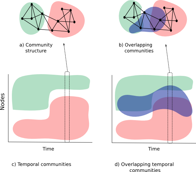
Knowing the OTC structure of an evolving network is useful because, although the observed network may change rapidly, its latent structure often evolves much more slowly. For example, contact-based social networks might change from day to day due to people’s varying daily activities, but the social groups (e.g. family, friends, colleagues) that people belong to are much more stable. Identifying such latent time-persistent structure can reveal the fundamental rules governing the seemingly chaotic evolution of real-life complex networks. In addition, knowledge of the times when significant changes occur could be used for predicting network evolution.
The OTC structure of networks has many applications to designing communication networks as well. For example, it can be used in efficient distributed storage of information in a wireless network so that average access latency is minimized [6]. The OTC structure can also be used to select relay nodes and design routing schemes in a disruption tolerant wireless networks. Another application is to devise real-life mobility models for analysis and evaluation of network protocols. We elaborate on these applications in Section VI.
Our approach: We describe the key ideas behind our techniques. A naive approach to temporal community detection is to perform static community detection independently in each snapshot. The limitations of this approach are well-documented [5], as it is very sensitive to even minor changes in the network. The approach can be extended to detect OTC structure as well but has the same limitations. Past work, including [2] and [5] argue that temporal communities can be detected if an explicit smoothness constraint that captures the distance to past partitions is enforced. With the smoothness constraint, it is possible to go beyond static methods and detect small persistent communities, as information at multiple snapshots is considered together. In this paper, we build on the above intuition and propose an approach for detecting OTC structure using temporal information. Our approach is a novel convex relaxation of the following combinatorial problem: find the temporal community structure that maximizes a quality function associated with each snapshot subject to a temporal smoothness constraint. To handle overlapping communities, we use generalizations of the quality function proposed in [7] and the temporal smoothness measure proposed in [5]. While the quality function favors densely connected groups, the smoothness constraint promotes persistent structure. Our formulation is fairly general and allows other quality functions and smoothness metrics to be used. Further, it is naturally applicable to overlapping temporal communities and does not require any ad hoc modifications. Unlike most existing approaches that use greedy heuristics to solve the resulting NP-hard problem of optimizing over the combinatorial set of all partitions (or covers when overlaps are allowed), we use a tight convex relaxation of this set via the trace norm. This not only results in a convex optimization problem that can be solved efficiently using existing techniques, but also enables us to obtain a priori guarantees on the performance of our method, and provides valuable insight. In particular, our analysis shows that, under a natural generative model, our method is able to recover communities that persists for snapshots and have size , where is the number of nodes. This result highlights the benefit of utilizing temporal information: with more snapshots, we are able to detect smaller communities. We believe this specific relation is novel, and applies beyond the particular methods in this paper. We note that our approach can detect non-overlapping temporal communities as well.
To summarize, we provide the first principled formulation of the problem of detecting overlapping temporal communities. A critical piece of the formulation is the quality function for quantifying the community structure in any snapshot, and a distance function to ensure contiguity with the past community structure. To the best of our knowledge, we are the first ones to propose such functions for overlapping communities. We provide a convex relaxation and hence an efficient way to solve the optimization problem, while most existing work relies on greedy heuristics. In addition, we provide theoretical guarantees on the performance of our method, and we discuss the insights we gain from the guarantees. Finally, we evaluate our method using several synthetic and real network data-sets and illustrate its efficacy. We also discuss applications of our method to communication networks.
Remark on terminology: In the sequel, we use cluster and community interchangeably, both allowing overlaps.
II Related Work
There is a long line of work on community detection which has been comprehensively surveyed in [1]. Here, we focus on work that is most relevant to our approach. In particular, [8] presents a convex formulation for optimizing modularity [9], a well-known quality function for static non-overlapping communities. Our convex formulation is completely different, and our allow overlapping and temporal communities. Our formulation is related to low-rank matrix recovery techniques [10, 11]. This line of work typically uses trace norm as a convex surrogate of the non-convex rank function, and similarly the norm for sparsity. In this paper, we use trace norm as a relaxation for the set of covers, a combinatorial and non-convex set, and the (weighted) norm as the quality function. Similar relaxation for static clustering without overlaps is considered in [12]. Our approach for dealing with overlaps is very different from exiting work; for a survey we refer to [13] and section XI of [1]. In the rest of this section we focus on an overview of temporal clustering.
Most existing work on temporal clustering can be divided into two categories: 1) maximize quality function subject to smoothness constraints; 2) slightly modify the clustering structure from the previous snapshot.
The first approach starts with [2], which proposes the framework of Evolutionary Clustering that aims to optimize a combination of a snapshot quality and a temporal smoothness cost. The work in [5] argues that a specific choice of the temporal cost, namely estrangement, works well. In [3] the authors uses the KL-divergence in both the snapshot quality and temporal cost, and reformulates the problem using non-negative matrix factorization in order to obtain soft clusterings. In [4] a particle-density based method is proposed to optimize the clustering objective. All of these works use greedy algorithms to solve the optimization problem, which only guarantees convergence to a local optimum. Our formulation is similar to the Evolutionary Clustering framework, but we are able to use convex optimization via a reasonable relaxation.
The second class of methods typically work as follows: each time the network changes, they modify the clustering structure to reflect the change according to some predefined rules. Smoothness is maintained since the modification would not change the clustering too much. For example, [14] proposes iLCD (intrinsic Longitudinal Community Detection) algorithm, which updates, merges, and creates communities based on the previous clustering; overlap is allowed. [15] adopts a similar idea, but does not allow a node to belong to multiple clusters while follow-up work [16] removes this restriction. However, all of these works use update rules that are based on heuristics; some of them might produce duplicates or very small communities and need to use ad hoc procedures to remove them. Unlike our work, they do not provide any analytical guarantees.
Other existing approaches include [17, 18, 19], which use objective functions that essentially measure both snapshot quality and temporal smoothness. Also, [20] propose a method to detect communities in multi-dimensional networks. None of these however detect overlapping communities and simultaneously detect their evolution over time.
III Formulation and Algorithm
In this section, we formulate the problem and describe our algorithm. We consider the following natural formulation of OTC detection. Suppose we are given snapshots of a network with nodes in terms of adjacency matrices , 111We use the convention .. Our general goal is, at each time , to assign each node to a number of clusters so that the edge densities within clusters are higher than those across clusters, and that the assignment does not change rapidly with time. Note that each node might be assigned to multiple clusters, and clusters can overlap. A node might also be associated with no cluster; these nodes are called outliers, and are common in real networks. Mathematically, let be the total number of communities at time . the value of is, of course, not known a priori. We would like to find covers with outliers, where a cover with outliers means a collection of subsets with ; again note that we allow outlier nodes that do not belong to any of the subsets. For convenience, we will use cover in the sequel when we actually mean cover with outliers.
To make this formulation concrete, there are several questions that need to be answered. 1) How to concisely represent a cover? 2) When overlaps are allowed, how to measure the quality of a cover? 3) In particular, how to avoid degenerate solutions? For example, declaring each edge as a cluster would make the in-cluster edge density and across-cluster density , but is an undesirable solution providing little information. Similarly, producing a cluster that differs from another only by one node hardly reveals any additional structure. 4) How to enforce temporal smoothness when overlap is present? 5) How to solve the resulting optimization problem over covers?
In the remainder of this section, we present our precise approach and address the above questions.
III-A Cover Matrix
Our first step, and also a key to later development, is to adopt a matrix representation of a cover. We use the following representation from [7].
Definition 1 (Matrix Representation of a Cover).
A matrix represents a cover if . That is, equals the number of clusters that include both node and .
Each cover has a unique matrix representation. To see this, let us introduce the notion of a cluster assignment matrix.
Definition 2 (Cluster Assignment Matrix).
is the cluster assignment matrix of a cover if when and zero otherwise.
The cluster assignment matrix is another representation of a cover which shows the clusters that each node belongs to. Clearly each cover corresponds to a unique , and each corresponds to a unique via the factorization (the -th entry of the matrix is the inner product of the -th and -th rows of , which, due to the structure of , equals the number of shared clusters of node and , i.e., ). In the sequel we will mainly use as the optimization variable, but the factorization is useful later for post-processing.
Another way to view the cover matrix is that it assigns to each pair of nodes a “similarity level” , measured by the number of shared clusters between and [7]. When there is no overlap, the assigned similarity level is either ( assigned to the same cluster) or (assigned to different clusters). When overlaps are allowed, nodes sharing many clusters are considered more similar. In contrast, the network adjacency matrix can be viewed as the observed similarity level. With this in mind, we can think of the general objective of OTC detection as: find a series of covers such that the assigned similarity level is closed to the observed one at each , and the covers change smoothly over time. In general the number of clusters that include both node and might be greater than , so the assigned similarity is also above .
III-B Overlapping Temporal Community Detection
We now give a precise formulation of the above general objective. We adopt an optimization-based approach to OTC Detection. In particular, we consider the following framework:
| (1) | |||||
| s.t. | |||||
Here is the snapshot quality, which serves two purposes: 1) it measures how well the cover reflects the network , i.e., the closeness between the assigned similarity level encoded in and the observed similarity level in , and 2) it prevents the algorithm from over-fitting, e.g., generating duplicate communities or many small communities overlap with each other. The function is a distance function that measures the difference between the covers at time and . Consequently, the first constraint in the above formulation ensures that the covers evolve smoothly over time. This constraint prefers the evolutionary path with fewer changes and reflects the inertia inherent in evolution of groups in real life networks.
In this paper we focus on concave and convex (w.r.t. ). This covers many existing methods for clustering without overlap. For example, can be the modularity function [9] (here is the degree of node in , is the total number of edges, and we ignore the pre-constant) or the correlation clustering [21] objective (here is called the matrix norm of ), and can be the estrangement [5] .
For OTC detection, the difficulty lies in defining quality and distance functions that can handle overlaps. We propose two novel metrics that are suitable to this task. For the snapshot quality , we use the weighted distance between the cover matrix and the adjacency matrix :
where are some weights to be chosen. In this paper, we use the weights , where and are defined in the last paragraph. This qualify function generalizes the correlation clustering objective [21] and is closely related to the widely-used modularity quality function [9] when there is no overlap. In particular, it penalizes three types of “errors” (recall is the number of clusters including both and , or the assigned similarity level between ):
-
•
and : nodes and are connected but they are assigned to different clusters
-
•
and : nodes and are disconnected but they share at least one clusters, i.e., the assigned similarity level is positive while the observed one is zero.
-
•
and : nodes and are connected but they share more than one clusters, i.e., the assigned similarity level is higher than the observed one.
Note that in the last two cases, the more clusters and share, the higher the cost is. This prevents the algorithm from over-fitting by generating many small clusters with lots of overlap.
For the temporal distance , we use:
In other words, we measure the change in the assigned similarity level between node and (i.e., the number of clusters that include both nodes), but only when there is an edge between and in both snapshots and . For non-overlapping clusters, this reduces to the number of persisting edges that change “state” from intra-cluster to inter-cluster and vice-versa. Our measure is a modification and generalization of the estrangement measure in [5] to overlapping clusters.
III-C Convex Relaxation
The optimization problem (1) is combinatorial due to the constraint “ represents a cover”. Exhaustive search is impossible because there are exponentially many possible covers. One option is to use greedy local search, which a popular choice for optimizing modularity and other clustering objectives, but it only converges to local minimums and provides no guarantees.
In this paper, we use convex optimization. There are two advantages of this approach: 1) it leads to an optimization problem that is efficiently solvable and guaranteed to converge to the global optimum, and 2) it is possible to obtain a priori characterization of the optimal solution (see Section IV), which provides interesting insights into the problem. To this end, we relax the cover constraint and solve the following optimization problem:
| (2) | |||||
| s.t. | |||||
here is the so-called trace norm, the sum of singular values of . It is known that the trace norm constraint is a convex relaxation of the original cover constraint [7]. We briefly explain the reason here. Recall that a cover matrix admits the factorization , so a cover is positive semidefinite and satisfies
| (3) |
In particular, the right hand side in (3) equals if represents a partition. Therefore, as long as is no smaller than the right hand side in (3), then a cover matrix also satisfies the new constraint, which is thus a relaxation. Although the right hand side in (3) is unknown a priori, in practice we find that choosing to be suitably large, such as as is done in our experiment section, works well. Moreover, the constraint effectively imposes an upper bound on the amount of overlap and prevents the algorithm from producing a large number of clusters, which is desirable on its own right.
Trace norm is known to be a good relaxation for partition matrices both in theory and in practice [22, 12]. All partition matrices with a small number of partitions (which is the case of interest) are low-rank, and trace norm is the tightest convex relaxation of low-rank matrices in a formal sense [23]. Moreover, trace norm utilizes the graph eigen-spectrum which has long been known to reveal hidden clustering structure and is the basis of the highly successful spectral clustering methods. This advantage of trace norm carries over to overlapping clusters [7]. With this relaxation and our choice of and , (2) becomes a convex program and can be solved in polynomial time using general-purpose convex optimization packages such as SDPT3. In Appendix -A, we describe a specialized gradient descent algorithm, which is even faster.
III-D Post-processing
Ideally, the optimal solution would represent a cover, which could be easily extracted from (e.g. by finding all maximal cliques); in the next section we provide one sufficient condition for this to happen. In practice, however, because of the relaxation, may not have the structure of a cover matrix. But it is empirically observed that is usually close to a cover matrix; in particular, the optimization can be viewed as a “denoising” procedure, which filters out most (though not all) of the noise in the observation and makes the underlying clustering structure more clear. Therefore, a good clustering is likely to be extracted from via simple post-processing. We describe one such procedure below.
Recall again that a cover matrix can be factorized as , where is an assignment matrix of non-negative entries, with indicating node in cluster . Therefore, performing Non-negative Matrix Factorization (NMF) [24] on a cover gives the corresponding clustering assignment. When the optimal solution is not an cover but close to be one, we expect that performing NMF would still produce an approximate assignment matrix , which is then rounded to be an exact assignment matrix. In particular, we declare node to belong to cluster at time if .
III-E Remarks on Our Method
Mapping communities: Practical application sometimes requires the communities at time to be mapped to those at , in order to track the evolution of communities. In the experiment section, we use the mapping method in [5], which still works when is a cover instead of a partition. The method involves mapping those communities across consecutive snapshots that have the maximal mutual Jaccard overlap between their constituent node-sets, and generating new community identifiers only when needed.
Online algorithm: In some cases it might be interesting to use an online version of the algorithm (2): At each time when a new snapshot becomes available, we obtain a new cover by solving the following problem:
| (4) | |||||
| s.t. |
where is the solution from the last snapshot and is considered fixed. Rigorously speaking, the solution to the online formulation is in general different from that to the offline one. But we expect in practice the online formulation will perform reasonably well, and various updating rules can be adopted to choose the online upper bound . We do not delve into this in this paper.
Complexity and Scalability: Using the fast gradient descent algorithm, the space and time complexities of our method both scale linearly with the problem size (the numbers of nodes, edges and snapshots); see Appendix -B for details. With the online implementation suggested above, the dependence on the snapshot number can be further alleviated. Our method is therefore amenable to large datasets.
IV Theoretical Analysis
In this section we provide theoretical analysis on the performance of our algorithm. In particular, our analysis shows that if the adjacency matrices are generated from an underlying persistent partition according to a generative model, then with high probability our method will recover the underlying partition as long as , where is the minimum cluster size in the partition and is the number of snapshots it persists for. This highlights the benefit of temporal clustering: a small cluster of size is likely to be undetectable if each snapshot is considered individually (e.g., the cluster might not be connected in each single snapshot), but can be recovered by temporal clustering if the cluster persists for snapshots and all snapshots are used. This result is quite revealing: traditional single-snapshot clustering techniques can only find clusters that are large in size, but temporal clustering is capable of detecting clusters that are small in size but large in the time axis. Moreover, our theorem predicts a specific tradeoff between the “spatial size” and the “temporal size” : with four times more temporal snapshots, one can detect a cluster that is half as small spatially. We believe this is the first such result in the literature.
We now present our theorem. We use a generative model which can be considered as a multi-snapshot version of the classical and widely studied planted partition model (a.k.a. stochastic block model) [25].
Definition 3 (Multi-Snapshot Planted Partition Model).
Suppose nodes are in disjoint clusters, each with size , and this clustering structure does not change over time (see remarks after the theorem). Let be the matrix that represents this clustering. The adjacency matrices are generated as follows: if node and are in different clusters, then there is an edge between them (i.e. ) with probability , independent with all others; if they are in the same cluster, then with probability . We assume are constants independent of , and .
Since the underlying partition does not change, we impose the constraint , which is equivalent to . Rewritten in an equivalent minimization form, our algorithm becomes
| (5) | |||||
Note that under the multi-snapshot planted partition model, we have , where . The following theorem characterizes when (5) recovers true underlying partition matrix .
Theorem 1.
Suppose . Under the multi-snapshot planted partition model, if , then is the unique optimal solution to the convex optimization problem (5) with probability converging to as .
The proof is given in Appendix -C.
Remark on Theorem 1: Although the multi-snapshot planted partition model assumes that the underlying clustering structure does not change, and that the clusters do not overlap, we conjecture similar theoretical guarantees can be obtained with these restrictions removed. In particular, we expect that our algorithm can detect clusters of size even if the underlying structure changes, provided that between consecutive changes there are at least snapshots. This conjecture is supported by the experimental results in section V.
V Experimental Results
We apply our method to two synthetic datasets and three real-world datasets. Our synthetic networks are random graphs generated according to an underlying community structure evolution. Each snapshot is an instantiation of a random graph generated by connecting each pair of nodes sharing at least one community with probability 0.5, and with probability 0.2 otherwise (including the case where one or both of the nodes are not in any community). Note that we allow some nodes in some snapshots to not belong to any community, as is often true in real scenarios. Also, note that nodes sharing more than one communities are not connected with a higher probability. This makes overlapping communities harder to detect and is a better test of the detection methods.
Using this prescription, we generate two synthetic time-varying networks to validate our method and demonstrate its efficacy. We compare the results obtained with and without overlap allowed, and with and without the smoothness constraint. A popular temporal clustering method using multi-slice modularity [19] is also considered.
The four real network datasets considered in this section include MANET, international trade, AS links, and the MIT Reality Mining Data.
V-A Synthetic Random Networks I
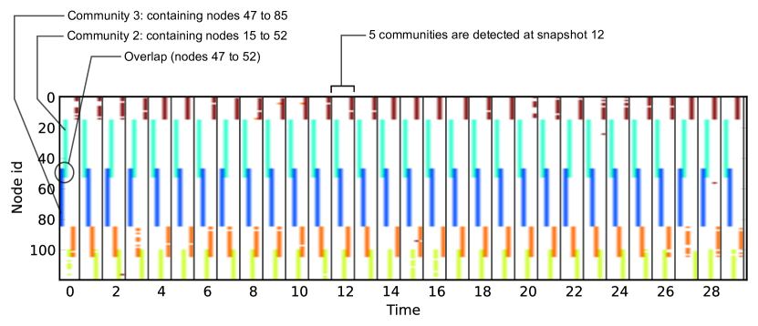
In the first synthetic experiment, we demonstrate the advantage of considering the temporal aspect and allowing overlap, and that there is clustering structure that can be detected only if we consider both. We generate the network snapshots as follows. Suppose there are 120 nodes and 5 underlying communities. Community 1 is a small 15-node group including nodes 0 through 14. Community 2 and 3, both of size 38, consist of nodes 15-52 and 47-85, respectively, and overlap at 5 nodes (47-52). Communities 4 and 5, both of smaller size 20, include node 85-104 and 100-119, respectively, and overlap at 5 nodes (100-104).
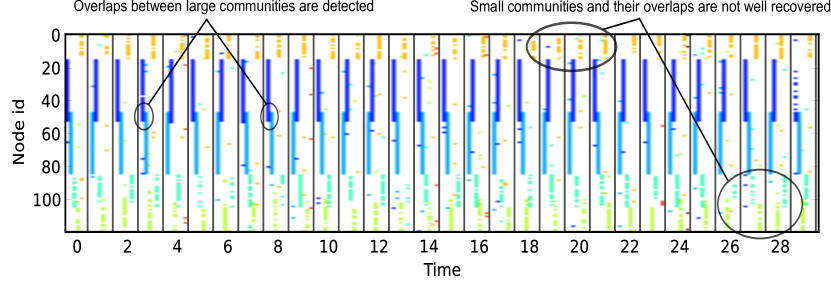
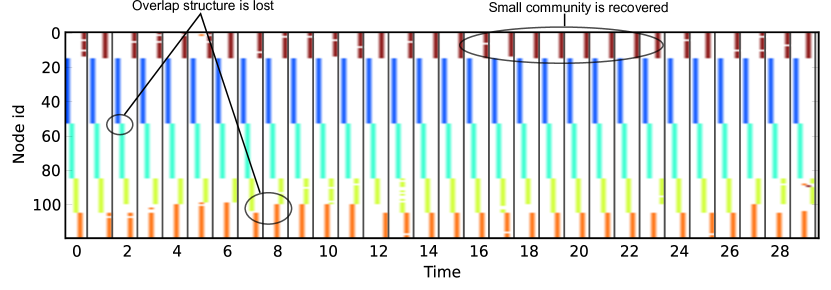
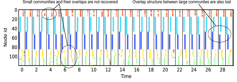
Since community 1 is small, in light of Theorem 1, we expect that single-snapshot methods are unable to detect it due to noise/randomness in the network, but temporal methods will find them. Community 2 and 3 are large but overlap with each other, so only methods that allow overlap would detect them, even if the snapshots are considered individually. Finally, communities 4 and 5 are small and overlapping, and are thus expected to be discoverable only when both the temporal and overlap aspects are considered. This is indeed the case in our experiments. The results are shown in Fig 2 to 5. Visualizing overlapping temporal communities is not a trivial task. Here we extend the approach used in Fig. 1 to allow overlaps, which is explained in the caption of Fig 2. Fig 2 shows the results of our method, which nicely detects all the underlying structure. Fig 3 shows the result of our method but with set to infinity, so there is no temporal smoothness constraint and snapshots are considered independently. In this case, communities 1, 4 and 5 are not recovered completely. Fig. 4 shows the result when overlap is not allowed, i.e., we impose the constraint . All overlapping structure is clearly lost. Fig 5 shows that result when and overlap is not allowed; one can see a further degradation of performance.
We also measure the performance of the above four methods by computing the distance of the recovered community structure from the ground truth. We use the distance , where denotes the cover matrix of the ground truth, and the one found by a clustering algorithm. The results are given in the second row of Table I. The error is an order of magnitude smaller when both the overlapping and temporal aspects are considered.
Comparison with existing schemes: Although there has been much work on community detection algorithms, almost none allows simultaneously discovering overlapping and temporal communities. Thus, we can only compare against some representative non-overlapping temporal community detection algorithms. We compare against the widely cited temporal community detection scheme presented in [19]. This method involves two parameters, the resolution for the modularity function and the inter-slice coupling strength . Since the ground truth clustering structure does not change over time, a large is used to force a static output. We then search over different values of and use the one that gives the smallest error. The recovered community structure is shown in Fig. 6. We find that this method cannot identify the overlap structure (as expected), and fails to recover the non-overlapping portions of small communities (community 4 and 5). The recovery error, given in the last column of Table I, is also high.

| Overlap+ temporal | Overlap only | Temporal only | None | Ref. [19] | |
|---|---|---|---|---|---|
| Expt I | 3133 | 27203 | 20646 | 32789 | 27390 |
| Expt II | 1646 | 14843 | 8318 | 12534 | 7450 |
V-B Synthetic Random Networks II
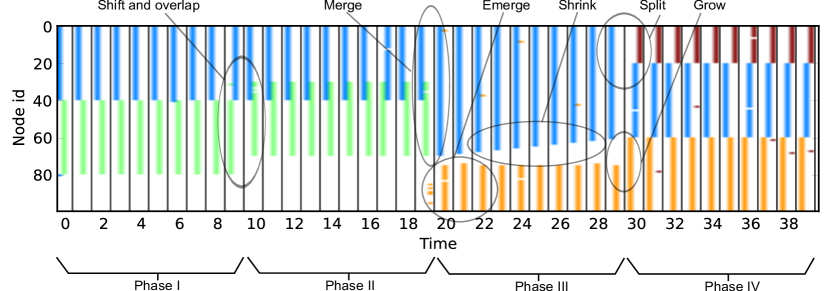
The second synthetic experiment demonstrates the ability of our method to detect and track time-varying cluster structure, including the overlap, merger, emergence, splitting, growth, and shrinking of communities. We describe how we generate the snapshots. The network has 100 nodes, and the underlying clustering structure has four phases, each with 10 snapshots:
-
•
Phase I: There are two communities: community 1 includes nodes 0 to 39, and community 2 includes nodes 40 to 79. The structure does not change during this phase.
-
•
Phase II: Community 1 remains the same, but community 2, now with nodes 30 to 69, overlaps with community 1. The structure does not change during this phase.
-
•
Phase III: Communities 1 and 2 merge into a large community A, which consists of nodes 0 to 69. This community then gradually shrinks: at each time there is one node leaving, and at the end of this phase, community A has nodes 0 to 60. On the other hand, there is a new community B, including nodes 75-99, emerges at the beginning of this phase and remains unchanged throughout this phase.
-
•
Phase IV: Community A splits into two smaller ones consisting of nodes 0-19 and 20-59, respectively. Community B grows by absorbing nodes 60-74, and thus has nodes 60-100. The structure does not change in this phase.
As can be seen in Fig. 7, our method performs quite well in recovering the underlying evolving structure. This complements our theoretical results in section IV, and shows that our method can handle overlaps and detect jumps in the structure. We compare our method with those that do not allow overlap, or ignore the temporal aspect; see Table I. Our method again outperforms other methods by a large margin.
Comparison: We also compare with the algorithm in [19]. For this algorithm, we search for the best parameters that give the smallest error. The recovered community structure is shown in Fig. 8, and the error is given in the last column of Table I. One observes that it cannot detect overlaps. Without considering overlaps, our method is competitive with a state-of-the-art algorithm that specializes for temporal clustering.

V-C Real MANET Scenario
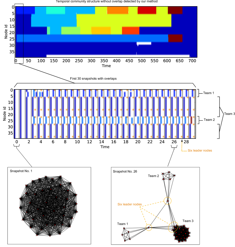
We now present results on a real wireless network with mobility. The data is based on the mobility trace from an experiment scenario in New Jersey as described in [26]. We use a 40 node version of the scenario where the nodes are organized into three teams. The teams move from an initial point to a target point using two primary routes over a three-hour period. The scenario is divided into several phases, each associated with a rendezvous point. During each phase the teams move from one rendezvous point to the next and pause before moving on. There are also six leader nodes which have high range radios and are mostly in range of each other.
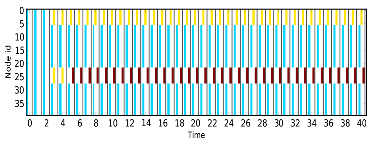
The input to our algorithm is 711 network snapshots formed by the wireless connection between the nodes. The physical locations of the nodes, as well as the underlying team structure, is unknown to the algorithm. The community structure found by our algorithm is shown in Fig. 9. We find that the leader nodes form a small yet persistent community (shown in orange in Fig. 9), which can only be detected by our clustering method. We also find that the overlapping temporal community structure is basically invariant for each phase of scenario even when the topology as well as the instantaneous community structure without overlap is changing. Thus, we show that in this case the overlapping temporal community structure detected by our method reveals a structural pattern that remains invariant even with a fair bit of mobility.
V-D MIT Reality-mining
We apply our method to a human-human contact network in the Reality-mining project [27]. The results are shown in Fig. 11. Two predominant groups can be seen, one corresponding to the staff at the MIT Media Lab, and the other corresponding to the students at the MIT Sloan School of Business. We also observe a discontinuity of the Sloan School community around New Year’s break.

V-E International Trade Network
Our next real dataset consists of annual trade volumes between pairs of countries during 1870–2006 [28]. We create an unweighted network each year by placing an edge between two countries if the trade volume between them exceeds of the total trade volumes of both countries; in other words, an edge is drawn if their trade is significant for both of them. This leads to a dynamic network with nodes and snapshots, which is fed to our algorithm.
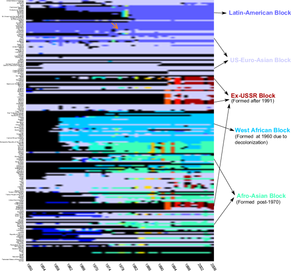
Fig. 12 shows the post-World War II (1950–2006) community structure found by our algorithm, where the overlaps are not displayed (for each node, only the largest cluster it belongs to is shown). Five prominent trade communities can be immediately identified: Latin-American, US-Euro-Asian, Ex-USSR Block, West African, and Afro-Asian. One also observes the evolution of the communities, including the formation of the West African block in 1960 (“the Year of Africa”) due to decolonization, the emergence of the Ex-USSR block after 1991, as well as Colombia and Venezuela joining the US-Euro-Asian Block in the 1970s.
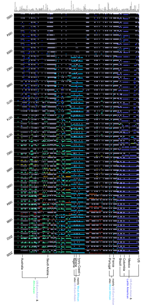
More information can be obtained by examining the overlap structure. A number of countries are associated with multiple communities. For example, US, Mexico, Colombia and Brazil belong to both US-Euro-Asian and Latin American blocks. France and Portugal are in the US-Euro-Asian block, but they both interact with the West African block for a significant number of years. Similarly, Ivory Coast, Ghana and Nigeria are mainly West African but also associated with the US-Euro-Asian. Several Asian/Pacific countries, including Saudi Arabia and Australia, have trade partners in both US-Euro-Asian and Afro-Asian blocks.
V-F The Skitter AS Links Dataset
Finally, to validate the performance of our algorithm on larger networks, we analyze the Internet topology at the Autonomous System (AS) level as collected by CAIDA [29]. We obtained quarterly snapshots of the data over an 8 year period starting in 2000. The data has upto 28000 nodes in some snapshots. Many of those are edge nodes with a low degree and do not belong to a community. Thus we only consider nodes with degree larger than in at least one snapshot. The final dataset consists of nodes and snapshots.
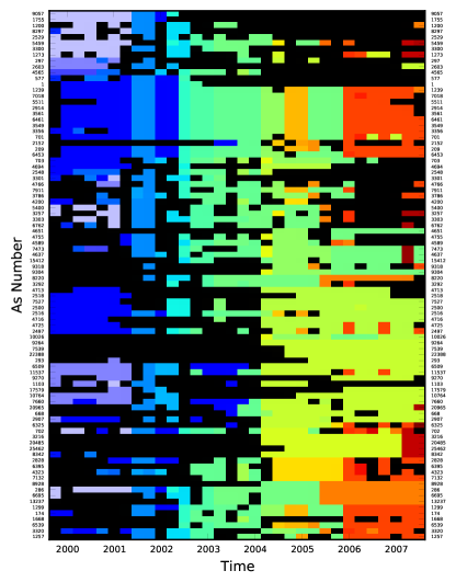
Among these AS’s, we identify 90 of them exhibit significant community structures – each of them are assigned to community in at least 10 snapshots. The temporal community structure for these nodes is shown in Fig. 14; overlaps are not shown for clarity. Results with overlaps are shown in Fig. 15.
We make some initial observations from Fig. 14: (1) In upper portion we see a persistent block with AS 1, 1239, 7018, 5511, 2914, 3561, 6461, 3549, 3356, 701, 209, and 6453. These seem to be mainly in US. (2) In the lower-right there is another smaller block with AS 8928, 286, 6695 and 13237, which seem to be EU and DE. (3) Between 2004 and 2005 there is some significant formation of new communities. A similar phenomenon has been observed in [30]. Moreover, by looking at the overlap structure, we find that that all the nodes in the US block mentioned above consistently appear in multiple clusters. These turn out to be Tier 1 providers or large internet exchange points.

VI Applications to Communication Networks
We now describe some applications of community detection to the design of communication networks.
Routing in Disruption Tolerant Networks (DTNs): DTNs are often formed by devices that are carried around by humans whose mobility patterns are strongly influenced by their social relationships. Thus, the structures of the social graph between the humans and the the contact graph between the devices are correlated. While the contact graph can change rapidly, it usually possesses a relatively stable underlying structure that is a function of the less volatile social graph [31, 32, 33, 34, 35]. This can be used to develop “social aware” routing strategies that use social metrics such as node centrality and community labels to make forwarding decisions [36, 31, 32, 33, 34]. All of these schemes utilize some form of community detection on the contact graph to infer social relations between the mobile nodes. However, the community detection methods used are generally limited to the non-overlapping and even non time-varying case. The community detection framework proposed in this paper can be used with any of these schemes while overcoming these limitations. This can result in significant performance gains when, for example, people belong to multiple social groups (e.g., friends, family, co-workers, etc.).
Efficient Caching in Content Centric Networks: Content based networking is an emerging paradigm that does not require connection oriented protocols between producers and consumers of information in communication networks. Intelligent caching and replication of the content can significantly reduce access delays as well as the overhead costs associated with repeated querying and duplicate transmissions. Recent work [6] proposes making use of the community structure of a MANET to determine nodes for content replication. Assuming that the community structure changes on a slower time scale than the network topology, nodes in the same community can cooperate to provide an efficient and speedy access to content. The method proposed in this paper can provide a principled approach to build distributed content caching protocols.
Developing Realistic Mobility Models: Much initial work on the design and analysis of routing algorithms for mobile networks assumed simplistic mobility models such as random walk, random waypoint, etc. However, the analysis of mobility traces from many real-life scenarios suggests that these simplistic models do not capture the details of real-world mobility characteristics such as periodicity and correlations due to social relationships between nodes. Recent work on mobility modeling [37, 38] attempts to capture the dependence of the social relationships between nodes on their mobility patterns. Community detection methods such as ours can be used to construct more refined mobility models that capture complex features such as the existence of overlapped communities as well as small yet persistent temporal communities.
VII Conclusion
In this paper, we consider the problem of detecting overlapping temporal communities in dynamic networks. A convex optimization based approach is proposed for this problem. Theoretical and experimental results show that our method is capable of revealing interesting community structure that cannot be detected by methods that do not allow overlap, or those that do not utilize temporal information. For simplicity, in this work we have focused on unweighted graphs. In the future, we plan to extend our method to treat weighted graphs as well as develop distributed versions of the algorithm. We believe our methods have wide applications in studying the structure and evolution of complex networked systems including communication networks and social networks.
Acknowledgements
Research was sponsored by the Army Research Laboratory and was accomplished under Cooperative Agreement Number W911NF-09-2-0053.
References
- [1] S. Fortunato, “Community detection in graphs,” Physics Reports, vol. 486, no. 3-5, pp. 75–174, 2010.
- [2] D. Chakrabarti, R. Kumar, and A. Tomkins, “Evolutionary clustering,” in ACM KDD, 2006.
- [3] Y.-R. Lin, Y. Chi, S. Zhu, H. Sundaram, and B. L. Tseng, “Facetnet: a framework for analyzing communities and their evolutions in dynamic networks,” in ACM WWW, 2008.
- [4] M. Kim and J. Han, “A particle-and-density based evolutionary clustering method for dynamic networks,” Proceedings of the VLDB Endowment, vol. 2, no. 1, pp. 622–633, 2009.
- [5] V. Kawadia and S. Sreenivasan, “Sequential detection of temporal communities by estrangement confinement,” Scientific Reports 2, 2012.
- [6] V. Kawadia, N. Riga, J. Opper, and D. Sampath, “Slinky: An adaptive protocol for content access in disruption-tolerant ad hoc networks,” in ACM Intl. Workshop on Tactical Mobile Ad Hoc Networking, 2011.
- [7] Y. Chen, H. Xu, and S. Sanghavi, “Graph clustering with overlaps,” Manuscript. Submitted.
- [8] G. Agarwal and D. Kempe, “Modularity-maximizing graph communities via mathematical programming,” The European Physical Journal B, vol. 66, no. 3, pp. 409–418, 2008.
- [9] M. E. J. Newman, “Modularity and community structure in networks,” PNAS, vol. 103, no. 23, pp. 8577–8582, 2006.
- [10] E. Candes, X. Li, Y. Ma, and J. Wright, “Robust principal component analysis?” Preprint arXiv:0912.3599, 2009.
- [11] V. Chandrasekaran, S. Sanghavi, S. Parrilo, and A. Willsky, “Rank-sparsity incoherence for matrix decomposition,” SIAM Journal on Optimization, vol. 21, no. 2, pp. 572–596, 2011.
- [12] Y. Chen, S. Sanghavi, and H. Xu, “Clustering sparse graphs,” Advances in neural information processing systems 25, 2012.
- [13] J. Xie, S. Kelley, and B. K. Szymanski, “Overlapping community detection in networks: the state of the art and comparative study,” To appear in ACM Computing Surveys, vol. abs/1110.5813, 2011.
- [14] R. Cazabet, F. Amblard, and C. Hanachi, “Detection of overlapping communities in dynamical social networks,” in IEEE SocialCom, 2010.
- [15] N. Nguyen, T. Dinh, Y. Xuan, and M. Thai, “Adaptive algorithms for detecting community structure in dynamic social networks,” in INFOCOM, 2011 Proceedings IEEE. IEEE, 2011, pp. 2282–2290.
- [16] N. Nguyen, T. Dinh, S. Tokala, and M. Thai, “Overlapping communities in dynamic networks: their detection and mobile applications,” in ACM Mobicom, 2011, pp. 85–96.
- [17] J. Sun, C. Faloutsos, S. Papadimitriou, and P. S. Yu, “Graphscope: parameter-free mining of large time-evolving graphs,” in ACM KDD, 2007.
- [18] J. Ferlez, C. Faloutsos, J. Leskovec, D. Mladenic, and M. Grobelnik, “Monitoring network evolution using MDL,” in IEEE ICDE, 2008.
- [19] P. Mucha, T. Richardson, K. Macon, M. Porter, and J. Onnela, “Community structure in time-dependent, multiscale, and multiplex networks,” Science, vol. 328, no. 5980, pp. 876–878, 2010.
- [20] Y. Chi, X. Song, D. Zhou, K. Hino, and B. Tseng, “On evolutionary spectral clustering,” ACM Trans on Knowledge Discovery from Data, vol. 3, no. 4, p. 17, 2009.
- [21] N. Bansal, A. Blum, and S. Chawla, “Correlation clustering,” Machine Learning, vol. 56, no. 1, pp. 89–113, 2004.
- [22] B. Ames and S. Vavasis, “Nuclear norm minimization for the planted clique and biclique problems,” Mathematical Programming, vol. 129, no. 1, pp. 69–89, 2011.
- [23] B. Recht, M. Fazel, and P. Parrilo, “Guaranteed Minimum-Rank Solutions of Linear Matrix Equations via Nuclear Norm Minimization,” SIAM Review, vol. 52, no. 471, 2010.
- [24] D. Seung and L. Lee, “Algorithms for non-negative matrix factorization,” Advances in neural information processing systems 13, 2000.
- [25] A. Condon and R. Karp, “Algorithms for graph partitioning on the planted partition model,” Random Structures and Algorithms, vol. 18, no. 2, pp. 116–140, 2001.
- [26] Y. Lu, F. Wicker, Y. Chen, P. Lió, and D. Towsley, “On secure network structures in the lakehurst trace,” 2008.
- [27] N. Eagle and A. Pentland, “Reality mining: sensing complex social systems,” Personal Ubiquitous Comput., vol. 10, pp. 255–268, 2006.
- [28] K. Barbieri and O. Keshk, “Correlates of war project trade data set.” [Online]. Available: correlatesofwar.org
- [29] B. Huffaker, Y. Hyun, D. Andersen, and kc claffy, “The Skitter AS Links Dataset.”
- [30] B. Edwards, S. Hofmeyr, G. Stelle, and S. Forrest, “Internet topology over time,” Preprint arXiv:1202.3993, 2012.
- [31] E. M. Daly and M. Haahr, “Social network analysis for routing in disconnected delay-tolerant manets,” in ACM Mobihoc, 2007, pp. 32–40.
- [32] P. Hui, J. Crowcroft, and E. Yoneki, “Bubble rap: Social-based forwarding in delay-tolerant networks,” Mobile Computing, IEEE Transactions on, vol. 10, no. 11, pp. 1576 –1589, nov. 2011.
- [33] W. Gao, Q. Li, B. Zhao, and G. Cao, “Multicasting in delay tolerant networks: a social network perspective,” in ACM MobiHoc, 2009.
- [34] A. Mtibaa, M. May, C. Diot, and M. Ammar, “Peoplerank: social opportunistic forwarding,” in IEEE INFOCOM, 2010.
- [35] A.-K. Pietilänen and C. Diot, “Dissemination in opportunistic social networks: the role of temporal communities,” in ACM MobiHoc, 2012.
- [36] Y. Zhu, B. Xu, X. Shi, and Y. Wang, “A survey of social-based routing in delay tolerant networks: Positive and negative social effects,” IEEE Comm. Surveys Tutorials, vol. PP, no. 99, pp. 1–15, 2012.
- [37] W.-J. Hsu, T. Spyropoulos, K. Psounis, and A. Helmy, “Modeling spatial and temporal dependencies of user mobility in wireless mobile networks,” IEEE/ACM Trans. Netw., vol. 17, pp. 1564–1577, 2009.
- [38] T. Hossmann, T. Spyropoulos, and F. Legendre, “Putting contacts into context: mobility modeling beyond inter-contact times,” in ACM MobiHoc, 2011, pp. 18:1–18:11.
- [39] N. Halko, P. Martinsson, and J. Tropp, “Finding structure with randomness: Probabilistic algorithms for constructing approximate matrix decompositions,” SIAM review, vol. 53, no. 2, pp. 217–288, 2011.
-A Fast Algorithm
Solving the program (2) using standard package is feasible only for small or medium size problems. In this section, we describe a faster algorithm that is suitable for larger scale datasets. Our method is based on matrix factorization. Each positive semidefinite cover matrix can be factorized as , where and . Here is any upper-bound on the number of clusters at each snapshot; one can always use , but a smaller value is more desirable. We consider the Lagrangian of the original constrained formulation. The optimization problem becomes
| (6) |
Choosing the multiplier is equivalent to choosing in the original formulation. We use (sub-)gradient descent to solve the problem:
| (7) |
where is the sub-gradient operator, denotes the (sub-)gradient w.r.t. the -th argument, is the Euclidean projection of onto the Frobenius norm ball (i.e., scale down to have Frobenius norm if and only if it is outside the ball), and is the step size. As for all gradient descent methods, the above procedure is guaranteed to converge provided . In this paper, we use a geometrically decreasing step size .
-B Complexity and Scalability
We analyze the memory and time complexity of the gradient descent algorithm.
Memory complexity: We need to store the adjacency matrices and the factorization , which requires and memory, respective; here is the total number of edges in all snapshots, the number of nodes, the maximum number of clusters at each snapshot, and number of snapshots. The total memory complexity is . The online implementation suggested in Section III-E will further alleviate the dependence on .
Time complexity: The algorithm requires time for computing a initial point, and for each iteration with iterations. Here we initialize by taking a rank- SVD of . For each this can be done in time (see [39]), where is the number of edges in snapshot . So . Now consider the update (7). The computation of the product of three (sub-)gradient operators with takes time , and , respectively, by taking advantage of the fact that we can use any sub-gradient. The summation and the projection both take . We thus have . The total time complexity is then . Characterizing the number of iterations needed for a specified accuracy rigorously is difficult, However, as observed empirically in our simulations and many other studies, is independent of , and , and can be treated as .
In summary, with a bounded number of clusters , both the space and time complexity scale linearly in and . This is the best one can hope for, as it takes at least this much space and time to read the input and write down the final solution.
-C Proof of Theorem 1
The following lemma shows that it suffices to study the Lagrangian formulation. Recall that is the matrix norm of . Let denote the entry-wise product.
Lemma 1.
is the unique optimal solution to (5) if there exists a such that is the unique optimal solution to the following problem
| (8) |
Proof.
Let and . Note that . By standard convex analysis and the fact that is optimal to (8), we have the following chain of inequality:
Therefore, equality holds above, which proves that is an optimal solution to (5). We prove uniqueness by contradiction. If is not the unique optimal solution to (5), then there exists with and . Using the equality we just proved, we have
which contradicts the assumption that is the unique optimal solution to (8). ∎
To prove Theorem 1, it suffices to show that is the unique optimal solution to (8) with . We do this by showing that any other solution with has a higher objective value.
We define a matrix which serves as a dual certificate. Let , , , and be the matrix whose columns are the singular vectors of . For any entry set , let denote the matrix whose entries in equals and others . Define , where
Due to the randomness in , both and are random matrices with independent zero-mean entries, whose variances are bounded by and due to the setup of the model. Under our choice of and the assumption of the theorem, they are further bounded by . Let be the spectral norm (the largest singular value). Standard bounds on the spectral norm of random matrices guarantees that with probability converging to one,
It follows that is a subgradient of , which means for all . Also define , where is the signum function, so . We also know is a subgradient of , so . Combining the above discussion, we have
We bound each of the above two terms. Notice that
here is the matrix norm. Under the assumption of the theorem, we have
and
Moreover, observe that each entry of , which is the sum of independent random variables with bounded variance as previously discussed. Under the assumption of the theorem, this sum is bounded by with probability converging to one by standard Bernstein inequality; is bounded by the same quantity using a union bound. It follows that
On the other hand, we have
Combining pieces, we obtain
This completes the proof of the theorem.