Low-temperature hopping dynamics with energy disorder: Renormalization group approach

Abstract

We formulate a real-space renormalization group (RG) approach for efficient numerical analysis of the low-temperature hopping dynamics in energy-disordered lattices. The approach explicitly relies on the time-scale separation of the trapping/escape dynamics. This time-scale separation allows to treat the hopping dynamics as a hierarchical process, RG step being a transformation between the levels of the hierarchy. We apply the proposed RG approach to analyze hopping dynamics in one- and two-dimensional lattices with varying degrees of energy disorder, and find the approach to be accurate at low temperatures and computationally much faster than the brute-force direct diagonalization. Applicability criteria of the proposed approach with respect to the time-scale separation and the maximum number of hierarchy levels are formulated. RG flows of energy distribution and pre-exponential factors of the Miller-Abrahams model are analyzed.

I Introduction

Understanding the dynamics of diffusion and transport in systems and materials with disorder is of paramount importance in multiple branches of modern science and engineering. The areas where the disorder-related phenomena are ubiquitous include biology,Dill and MacCallum (2012) condensed matter physics,Levi et al. (2011) polymerLee et al. (2006); Nicolai et al. (2012) and nano science.Hermosa et al. (2013) Carriers of various nature can be involved into transport phenomena in different systems: excitons in molecular or semiconductor quantum dot aggregates and polymer chains/films; charge carriers (electrons or holes) in disordered semiconductors, phonons and photons in disordered heat conductors and photonic crystals, respectively.

The nature of disorder can also vary a great deal from system to system. One of the most important sources of disorder is the energy dispersion – the dynamics of a system occurs in a configuration space with a rugged landscape so that potential barriers have to be overcome, e.g., by an exciton to migrate within a polymer chain. Specifically, it is well documented that in amorphous conjugated polymers, excitons can be localized in short ordered segments of a polymer chain, where the energy of the exciton depends on the length of the segment giving rise to the energy disorder. An inevitable consequence is that the exciton, generated at an arbitrary site in the excitonic density of states distribution, will migrate (spectral diffusion) and, ultimately, tend to relax towards low-energy states.Arkhipov, Emelianova, and Bässler (2004); Ahn, Wright, and Bardeen (2007); Athanasopoulos et al. (2008); Köhler and Bässler (2011); Hwang and Scholes (2011) It has to be noted that in amorphous films of conjugated polymers the energy disorder can be strong in a sense that the site-to-site energy variation can significantly exceed $k_{B}T$ at room temperature.Meskers et al. (2001); Athanasopoulos et al. (2008) Possible mechanisms of exciton-exciton coupling between polymer segments include Förster resonance energy transfer (due to dipole-dipole Coulomb interaction),Förster (1948) as well as Dexter energy transfer (due to the direct overlap of electronic wavefunctions).Dexter (1953)

Exciton transport in aggregates of semiconductor quantum dots has received much attention lately because of multiple promising applications in photovoltaics, electronics and information processing. Within such aggregates, the energy of lowest exciton varies between quantum dots due to the quantum mechanical confinement of carriers in quantum dots with size distribution. J. L. Mohanan (2005); Gaponik, Herrmann, and Eychmuller (2012) In these systems, photoinduced excitons have been demonstrated to efficiently migrate within an aggregate.Crooker et al. (2002); Reitinger et al. (2011); Belyakov and Burdov (2011) One of the possibilities to make quantum dots “talk” to each other, i.e., to make an exciton migrate, is via aerogels - a special type of aggregates - which are of great promise for photovoltaic and thermoelectric applications.Ganguly and Brock (2011); De Freitas et al. (2012)

Diffusion and transport phenomena in the presence of disorder are often characterized by the absence of well-defined time, size or energy scales. The renormalization group (RG) approach is one of the most suitable methods to study dynamics under such conditions. The RG has been extensively applied before to study the diffusion in energy-disordered systems, however mostly for the case of weak disorder.Deem and Chandler (1994); Bouchaud and Georges (1990) Transport in the case of strong disorder, i.e., where the energy dispersion significantly exceeds the temperature (in energy units) of the environment, has been studied to a much lesser extent mostly due to the lack of appropriate methods.Bouchaud and Georges (1990) In this paper, we introduce the numerical real-space RG method capable of studying hopping diffusion in the presence of a strong energy disorder.

The rest of the paper is organized as follows. The notation and general theory is introduced in Section II. The RG transformation is described in Section III. General numerical results and the discussion of the RG flow are discussed in Secs. IV and V, respectively. Section VI concludes.

II Hopping on graph

We describe the hopping dynamics of a system with energy disorder as Markovian hopping between nodes of a graph, where the hopping probability is defined by rate constants assigned to edges of the graph [see Fig. 1(a) for graph schematics].

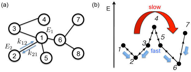
Figure 1: (a) Schematic of a graph for hopping dynamics. Rate constants are shown for an edge connecting nodes $1$ and $2$. (b) Schematic of hopping dynamics on the graph with two local energy minima. At low temperature, the relaxation dynamics within each minimum is expected to be mush faster than the subsequent population transfer between the minima.

Physically, each node of this graph can represent an ordered (i.e., unbent) segment of a polymer chain with kinks, so that at each moment of time an exciton is localized within a single segment. The time-dependent population is assigned to each node of the graph, representing the probability to find an exciton within the corresponding segment at a specific moment of time. The length dispersion of segments results in a variation of exciton energy, thus introducing the energy disorder. Accordingly, each node of the graph is parametrized with energy.

The probability for an exciton to hop from one node to another is specified by two hopping rate constants (forward and backward), which are assigned to each edge of the graph, as illustrated in Fig. 1(a) for nodes $1$ and $2$. An important characteristic of the so formed graph is its connectivity – the average number of edges connected to a node. In principle, a hopping rate constant can be non-zero between any two nodes of the graph, regardless of how distant they are from each other. A physical example of this is a non-vanishing exciton-exciton coupling between two very distant segments of a polymer chain, or between distant quantum dots within an aggregate. However, hopping rate constants typically decay rapidly with distance, $R$, e.g., as $\sim R_{0}^{6}/R^{6}$ in the case of the dipole-dipole (Förster) or $\sim e^{-R/R_{0}}$ in the case of the exchange-type (Dexter) interaction, where $R_{0}$ is a characteristic range of interaction. Henceforth, we allow edges to link only nearby nodes, thus restricting the graph connectivity to be finite even in the thermodynamic limit, where the number of nodes within the graph grows to infinity.

The hopping dynamics on the so introduced graph is governed by the following kinetic equation van Kampen (1992)

$$\partial_{t}|p(t)\rangle=\hat{W}|p(t)\rangle,$$ (1)

where $|p(t)\rangle$ is the vector of time-dependent node populations. We denote the projection of an arbitrary vector $|a\rangle$ onto node $i$ via $(i|a\rangle$, so that, e.g., $p_{i}(t)=(i|p(t)\rangle,~{}i=1,...,N$ ($N$ is the total number of nodes in the graph) is the population of node $i$ at time $t$. The rate matrix is constructed as follows.van Kampen (1992) Its off-diagonal elements read as

$$W_{ij}=(i|\hat{W}|j)=k_{ij},\,i\neq j$$ (2)

where $k_{ij}$ is the rate constant for hopping from node $j$ to node $i$ [see Fig. 1(a)]. The diagonal matrix elements are not independent and are determined from the population conservation condition, which requires the sum of elements in any column of $\hat{W}$ to vanish identically, yielding

$$W_{ii}+\sum_{j\neq i}W_{ji}=0.$$ (3)

Therefore, Eq. (1) is the gain-loss equation for populations of nodes.

An additional constraint imposed on the rate constants is the detailed balance

$$\frac{k_{ij}}{k_{ji}}=e^{-\beta(E_{i}-E_{j})},$$ (4)

where $\beta=1/k_{B}T=1/T$ ($k_{B}=1$ throughout the paper). The energy of node $i$ is denoted by $E_{i}$. Eq. (4) guarantees that state $(i|p_{eq}\rangle\propto e^{-\beta E_{i}}$ is the equilibrium state of the system, i.e., it is the steady state solution of Eq. (1), $\partial_{t}|p(t)\rangle=0$, with no currents.

Eq. (1) can be formally solved as $|p(t)\rangle=e^{\hat{W}t}|p_{0}\rangle$, where $|p_{0}\rangle=|p(t=0)\rangle$ is the vector of initial populations. The rate matrix, satisfying Eqs. (3) and (4), can be diagonalized as $\hat{W}|n\rangle=-\lambda_{n}|n\rangle$,van Kampen (1992) yielding

$$|p(t)\rangle=\sum^{N-1}_{n=0}|n\rangle\langle n|p_{0}\rangle e^{-\lambda_{n}t}.$$ (5)

Here, we note that since $\hat{W}$ is not symmetric, both right and left, i.e., $\langle n|\hat{W}=-\langle n|\lambda_{n}$, eigenvectors have to be found. Because of the detailed balance, all the eigenvalues are strictly non-negative and the lowest eigenvalue is always zero, $\lambda_{0}\equiv 0$, corresponding to the equilibrium. The normalized right and left eigenvectors corresponding to this equilibrium mode, $n=0$, are $|0\rangle=Z^{-1}\sum_{i}|i)e^{-\beta E_{i}}$ and $\langle 0|=\sum_{i}(i|$, respectively. The partition function is given by $Z=\sum_{i}e^{-\beta E_{i}}$.

Eq. (5) completely solves the problem defined by Eqs. (1)-(4) , since any observable which depends on node populations at an arbitrary moment of time can now be expressed via Eq. (5). For example, the average energy of an exciton at time $t$ is given by

$$\langle E(t)\rangle\equiv\frac{\langle E|p(t)\rangle}{\sum_{i}(i|p(t)\rangle}=\frac{\sum_{n}\langle E|n\rangle\langle n|p_{0}\rangle e^{-\lambda_{n}t}}{\sum_{i}(i|p_{0}\rangle},$$ (6)

where $\langle E|$ is the vector of node energies, i.e., $\langle E|i)=E_{i}$. Deriving Eq. (6), we explicitly used the population conservation requirement.

III Coarse graining

Eq. (5) is an exact solution of the problem of hopping dynamics on a graph. However, this solution might not be optimal for the following reasons. First, the dispersion of node energies, $E_{i}$, leads to the emergence of local minima where the population can be trapped at low temperatures. From the perspective of diagonalization of rate matrix $\hat{W}$, it results in a very broad spectrum of eigenvalues and, therefore, coexistence of different timescales. The relaxation within local minima occurs rapidly, but the population transfer between local minima is slow due to the necessity to overcome potential barriers. This is illustrated in Fig. 1(b), where relaxation within local minima (1-2-3 and 5-6-7) can be fast, but it is hard to overcome the potential barrier (3-4-5) at low temperatures, which results in a very slow inter-minimum transfer. The natural criterion for the separation of timescales for these two processes can be introduced as $\gamma=\delta E/T\gg 1$, where $\delta E=\left[N^{-1}\sum_{i}\left(E_{i}-\bar{E}\right)^{2}\right]^{1/2}$ is the standard deviation of node energies, and $\bar{E}=N^{-1}\sum_{i}E_{i}$ is their mean. At $T\ll\delta E$ the eigenvalues of $\hat{W}$ can be spread over many orders of magnitude, rendering the numerical diagonalization of the rate matrix inaccurate due to numerical round-off errors.

The second reason is that the existence of a small parameter, $1/\gamma$, might simplify the solution and analysis of the problem, and also might allow one to treat much larger systems than those dealt with by the brute-force direct numerical diagonalization. Similarly to how the introduction of a small parameter simplifies a problem in quantum mechanics by allowing for a perturbative solution, we intend to explicitly use the smallness of $1/\gamma$ to simplify the solution of the problem and make it more physically transparent.

A straightforward approach is to explicitly separate the time scales by first solving for population relaxation dynamics within each local minima. Then, the inter-minima transfer problem is solved considering population in each minima to be in its own quasi-equilibrium. This is similar to transition state theory, where the timescale separation allows one to consider both reactants and products equilibrated within respective potential wells.Hänggi, Talkner, and Borkovec (1990) Using the analogy between energy dispersion of the graph and rain/water collection in a rugged landscape we will refer to local minima as drainage basins or simply basins. Thus, we propose to divide the entire graph into a collection of basins, and first solve for the population dynamics within each basin independently. Then, the population is considered to be equilibrated within each basin and dynamics of population transfer between basins will be solved for. To make a step further, one can notice that the population transfer between the equilibrated basins can be again treated as a Markovian hopping process on a new graph which describes inter-basin hopping dynamics. This new graph can be thought of as a result of coarse-graining of the initial graph. The construction of this new graph out of the initial one is essentially an RG transformation (or step) applied to the original graph. This RG step can be performed multiple times consecutively giving rise to a hierarchy of levels of coarse-graining. At each such level, the population is being transferred between nodes, and each of these nodes represents an“equilibrated” basin of the graph belonging to the previous hierarchy level. Fig. 2 schematically depicts the consecutive RG transformations applied to the original (microscopic) graph.

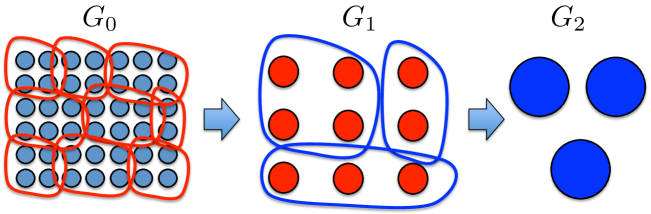
Figure 2: Schematic representation of consecutive RG transformations leading to a hierarchy of coarse-graining levels. Closed contours show how nodes are combined into basins.

In this figure, the microscopic graph is denoted by $G_{0}$. The basins of this graph are outlined by the red contours, and upon the RG step, each basin within $G_{0}$ becomes just a single node (red circle) in a new graph, $G_{1}$. Once $G_{1}$ is constructed, the RG transformation can be applied to this new graph, yielding $G_{2}$ and so on. In what follows, each graph within the RG hierarchy will be designated by $G_{h}$, where index $h$ stands for the number of RG transformations applied consecutively to the original graph $G_{0}$. The ordered set (lowest to highest) of the exact eigenvalues of graph $G_{h}$ (e.g., obtained via numerical diagonalization) is denoted by $\Lambda_{h}=\left\{\lambda_{1},\lambda_{2},...,\lambda_{N}\right\}$. The set of eigenvalues corresponding to relaxation within basins of $G_{h}$ is denoted by $\Lambda^{\prime}_{h}$. Thus, the number of elements in $\Lambda^{\prime}_{h}$ and $\Lambda_{h}$ is different by the number of basins in $G_{h}$. Further, we introduce a notation for the entire spectrum of the system, obtained by $H$ successive RG transformations, as

$$S_{H}=\bigcup_{h=0}^{H-1}\Lambda^{\prime}_{h}\cup\Lambda_{H}.$$ (7)

If RG transformations were exact, the following equality would hold

$$S_{0}=S_{1}=S_{2}=...$$ (8)

Since an explicit timescale separation is approximate, and therefore also the RG transformation, the validity of this expression depends on the magnitude of $\gamma$ at each level of the hierarchy. In the remainder of the section we discuss the specific procedure of coarse-graining.

III.1 Single RG step

We propose the following algorithm for the coarse-graining procedure:

1. In the entire graph, nodes are identified which are linked only to nodes of higher energy. Each such low-energy node will be called the “seed” of a basin.

2. For any other node of index $i$, a node $j$ is found so that the following requirements are satisfied: (i) there exists an edge linking nodes $i$ and $j$, (ii) $E_{i}>E_{j}$, and (iii) of all indices $j$ satisfying the first two requirements we choose the one maximizing $k_{ji}$. If node $j$ has already been associated with any basin (e.g., node $j$ is a seed), we associate node $i$ with the same basin.

3. Repeat Step 2 until all the the nodes of the graph are associated with basins.

Step 1 finds all the seeds and associate them with basins yet to be “grown”. The first execution of Step 2 associates with basins only the nodes connected directly to basin seeds. Then, nodes connected to seeds through a single node (i.e., via two edges) are associated with basins and so on. At a very low temperature (i.e., $\gamma\gg 1$), this approach guarantees that a particle (e.g., an exciton), initially residing at node $i$, will preferentially relax to the seed of the basin node $i$ belongs to. Here, “preferential” means that we construct the basins using the maximum $k_{ij}$ requirement, neglecting all smaller $k_{ij}$. This can lead to a non-negligible probability of particle relaxation to other seeds. This is illustrated by initially putting an exciton on node $4$ of the graph shown in Fig. 1(b). As is seen, it can relax to both seeds $2$ and $6$, but we associate node $4$ with the left basin if $k_{34}>k_{54}$, and with the right basin if $k_{34}<k_{54}$.

Once basins are formed, we construct a rate matrix $\hat{W}^{b}$ for each basin ($b$ is the basin index) as if it is isolated from the rest of the graph. In other words, $k_{ij}$ is set to zero if nodes $i$ and $j$ belong to different basins. Then, a typically small rate matrix for each isolated basin is numerically diagonalized

$$\hat{W}^{b}|n,b\rangle=-\tilde{\lambda}_{n}^{b}|n,b\rangle,$$ (9)

where the lowest eigenvalue vanishes exactly ($\lambda_{0}^{b}=0$) because of the detailed balance, identically to the case of the entire graph (see above). The eigenvectors, corresponding to these quasi-equilibrium eigenmodes (one per basin), read as (right and left eigenvector, respectively)

$$(i|0,b\rangle =Z^{-1}_{b}e^{-\beta E_{i}}\delta_{i\in b},$$

$$\langle 0,b|i) =\delta_{i\in b},$$ (10)

where $\delta_{i\in b}$ equals $1$ if node $i$ belongs to basin $b$ and zero otherwise. The partition function of basin $b$ is given by $Z_{b}=\sum_{i\in b}e^{-\beta E_{i}}$. The left and right eigenvectors are obviously orthonormal, i.e., $\langle 0,b^{\prime}|0,b\rangle=\delta_{bb^{\prime}}$.

The problem of “preferential” relaxation can lead to a significant underestimation of eigenvalues corresponding to intra-basin relaxation, $\tilde{\lambda}_{n}^{b}$ ($n\neq 0$). Indeed, at very low temperatures the population of node 4 in Fig. 1(b) would decay with the rate constant of $k_{34}+k_{54}$. Associating node $4$ with a specific basin (left or right), as it is done in the coarse-graining procedure described above, would allow it to decay with rate $max(k_{34},k_{54})$ which can introduce a significant error up to a factor of $C$ - graph connectivity. Indeed, for the specific example discussed here (one-dimensional graph, $C=2$), one has

$$max(k_{34},k_{54})\leq k_{34}+k_{54}\leq 2\times max(k_{34},k_{54}),$$ (11)

so if $k_{34}$ and $k_{54}$ are not too different, Eq. (9) produces significantly underestimated intra-basin eigenvalues. To correct for this, we recalculate eigenvalues of intra-basin relaxation modes as

$$\lambda_{n}^{b}=-\langle n,b|\hat{W}|n,b\rangle.$$ (12)

Using the language of perturbation theory in quantum mechanics, one can say that these new eigenvalues are first-order corrected relative to the zeroth-order approximation given by Eq. (9). Eigenvalues $\lambda_{n}^{b}$ ($n\neq 0$) constitute $\Lambda^{\prime}_{h}$ at a given hierarchy level $h$, and are not modified any more by any further (consecutive) RG transformations.

The rate matrix for the the coarse-grained graph, describing the population transfer between basins, is constructed as follows. The rate constants for population transfer between equilibrated basins are defined as

$$k_{b^{\prime}b}=\langle 0,b^{\prime}|\hat{W}|0,b\rangle=\sum_{i\in b^{\prime}}\sum_{j\in b}k_{ij}Z^{-1}_{b}e^{-\beta E_{j}}$$ (13)

Physically, this means that we take equilibrium populations of basin $b$ and multiply them by rates of population transfer to basin $b^{\prime}$. It is easy to see that

$$k_{b^{\prime}b}/k_{bb^{\prime}}=e^{-\beta(F_{b^{\prime}}-F_{b})},$$ (14)

where the Helmholtz free energy of a basin is defined as $F_{b}=-T\ln Z_{b}$. The new graph is the result of the RG transformation applied to the graph of the previous hierarchy level. It is constructed as:

1. Each node is the basin of the previous graph.

2. The energy of each node is the free energy of the equilibrated basin of the previous graph.

3. Rate constants of population transfer between nodes are given by Eq. (13)

4. Initial populations of each node of the new graph are given by $\langle 0,b|p_{0}\rangle$, where $|p_{0}\rangle$ is the vector of initial populations of the previous graph.

5. Time-dependent population of each node is interpreted as the total population of a corresponding equilibrated basin of the previous graph.

III.2 Consecutive RG steps as approximate diagonalization without dimensionality reduction

In contrast to standard RG procedures in statistical physics, where upon an RG step the microscopic information is typically lost, we can keep the entire spectrum of eigenvalues during the coarse-graining procedure. In the coarse-graining procedure we proposed above, the rate matrix $\hat{W}$ is partially diagonalized at each RG step in a sense that the first RG step applied to $\hat{W}$ transforms the rate matrix to a block-diagonal one. One of these blocks is exactly diagonal within, as it consists of eigenvalues $\lambda_{i}^{b}$ ($i\neq 0$), corresponding to the intra-basin relaxation. The other block, non-diagonal within, is the rate matrix for inter-basin transitions, constructed out of rates defined by Eq. (13). Each consecutive RG step further decreases the size of this internally non-diagonal block and correspondingly increases the size of the internally diagonal one keeping the overall dimensionality of the full rate matrix the same. In other words, the RG approach introduced here is a method to approximately diagonalize a certain class of matrices such as rate matrix $\hat{W}$ at low temperature. It is, therefore, clear that Eq. (5) is still valid as long as the RG-based diagonalization of $\hat{W}$ is accurate. For example, Eq. (6) can still be used to find the time-resolved average energy of the system.

Clearly, only a finite number of consecutive RG transformations can be applied to a finite system, since the size of the graph is rapidly decreasing with each consecutive level of the hierarchy (see below). In fact, after a certain number of successive RG steps the direct diagonalization is typically possible even for a very large initial system. The validity and accuracy of the coarse-graining procedure can impose an additional constraint on the maximum number of RG steps. Indeed, $\delta E$ - energy dispersion of graph nodes - can be defined at each level of hierarchy, resulting in the whole set of perturbation parameters, $\{1/\gamma_{0},1/\gamma_{1},...\}$. Even if $1/\gamma_{0}$ is sufficiently small to guarantee the validity of coarse-graining of the original graph, RG might become inaccurate at hierarchy level $h$ when $1/\gamma_{h}$ is on the order of $1$. We discuss this issue in Sec. V.

IV Numerical results for coarse-graining

To demonstrate the validity of the proposed RG approach at low temperatures, we consider the following generic systems with energy disorder. Regular lattices, either one-dimensional chain (1D) or two-dimensional square (2D), are constructed. Only the nearest neighbors are linked and periodic boundary conditions imposed, forming graph $G_{0}$ with connectivity $C=2$ and $C=4$ in the 1D and 2D cases, respectively. Hopping rate constants are assigned to each edge of the graph by using the modified version of the Miller-Abrahams (MA) model Miller and Abrahams (1960)

$$k_{ij}=\begin{cases}k_{ij}^{0}\exp(-\beta\Delta E_{ij}),&\Delta E_{ij}>0\,({\rm{\rm up-hop}}),\\ k_{ij}^{0},&\Delta E_{ij}<0\,({\rm{\rm down-hop}}).\end{cases}$$ (15)

Node energies, $E_{i}$ ($i=1,...,N$), are assigned via sampling the Gaussian distribution with $\delta E=\langle(E-\bar{E})^{2}\rangle=1$. The mean node energy, $\bar{E}=N^{-1}\sum_{i}E_{i}$, is irrelevant for hopping dynamics since only relative node energies enter the expression for the rate constants.

In Eq. (15), a single pre-exponential factor is assigned to each edge

$$k_{ij}^{0}=k_{ji}^{0}=\exp(-\beta\epsilon_{ij}^{a}),$$ (16)

where $\epsilon_{ij}^{a}$ is an activation energy of the hopping along edge $(i,j)$. Activation energies are assigned via sampling the standard uniform distribution, $\epsilon_{ij}^{a}\rightarrow\mathcal{U}(0,1)$, so that $\epsilon_{ij}^{a}\in(0,1)$. The presence of this temperature-dependent pre-exponential factor makes Eq. (15) different from the classical MA model, the latter is recovered by setting all the activation energies to some fixed value, e.g., $\epsilon^{a}_{ij}=0$. The nature and implications of this modification are discussed in the end of Sec. V. In the rest of the section numerical results are presented for 1D and 2D systems with the rate constants specified by Eqs. (15) and (16).

IV.1 1D lattice

Fig. 3 presents the results of the RG-based calculations of the eigenvalue spectrum for a 1D system with 2500 nodes.

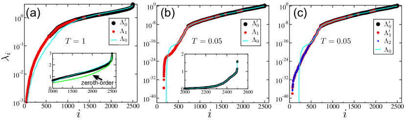
Figure 3: Comparison of the RG approach with direct diagonalization for the 1D chain, $\Lambda_{0}$. (a) Direct diagonalization versus a single RG step at high temperature ($T=1$). (b) Direct diagonalization versus a single RG step at low temperature ($T=0.05)$. (c) Direct diagonalization versus two RG steps at low temperature ($T=0.05$). Insets represent the same data as main graphs, but plotted in linear axes to emphasize the region of large eigenvalues. The inset in panel (a) also shows the eigenspectrum without the first-order perturbative correction of eigenvalues, obtained from Eq. (9) instead of Eq. (12).

Panel (a) shows the spectrum obtained by the direct diagonalization ($\Lambda_{0}$), as well as the RG approach with a coarse-graining ($\Lambda_{0}^{\prime}$, $\Lambda_{1}$) at a temperature equal to the magnitude of the energy disorder, i.e., $T=\delta E=1$. As expected, at $T/\delta E\gtrsim 1$ the performance of the RG approach is not perfect. Specifically, it underestimates the large eigenvalues originating with intra-basin relaxation (compare $\Lambda_{0}$ and $\Lambda^{\prime}_{0}$ in the inset at $i\sim 2300$), because an exciton can escape a basin on the same timescale as the intra-basin relaxation occurs, which increases eigenvalues of “intra-basin” modes. That RG neglects basin escape processes at short times ($\Lambda_{0}^{\prime}$) leads, in turn, to their effective emergence at long times ($\Lambda_{1}$), resulting in overestimated values for smaller eigenvalues (compare $\lambda_{i}$ at $i\sim 500$). In other words, the incomplete timescale separation at high temperatures can be thought of as an interaction between intra-basin relaxation and basin escape processes, which is not accounted for within RG. Treating this interaction within the second-order perturbation theory would shift high eigenvalues even higher, and low eigenvalues even lower, similarly to the standard second-order perturbative corrections to energy in quantum mechanics. Accordingly, RG underestimates high (intra-basin) and overestimates low (inter-basin) eigenvalues due to the lack of second-order perturbative corrections.

Numerical results for the significantly smaller temperature, $T=0.05$, are shown in panels (b) and (c). As is seen, the performance of the RG method improved, as compared to the large temperature case, as RG results nearly coincide with the direct diagonalization results for a large (higher) part of the spectrum [see also inset in panel (b)]. In fact, at such low temperatures the RG approach outperforms the direct diagonalization. The kink seen in the direct diagonalization spectrum at $\lambda_{i}\sim 10^{-18}$, followed by a rapid decrease, is due to numerical round-off errors: $\approx$220 eigenvalues turned out to be negative in $\Lambda_{0}$. In comparison, a single coarse-graining gives only $\approx$150 negative eigenvalues in $\Lambda_{1}$ [see panel (b)], which is seen by a lower position of the kink. Furthermore, two consecutive RG steps applied to $G_{0}$ result in only $\approx$50 negative eigenvalues in $\Lambda_{2}$, as is seen in panel (c) by the apparent absence of the kink and very low onset of the rapid decrease in the RG eigenspectrum.

The inset of Fig. 3(a) also shows the comparison of the first-order corrected eigenspectrum ($\Lambda^{\prime}_{0}$), defined by Eq. (12), and the zeroth-order eigenspectrum (green line), defined by Eq. (9). As was anticipated [see the discussion between Eq. (9) and Eq. (12)], the first-order corrected spectrum agrees better with the exact result, $\Lambda_{0}$, than the zeroth-order eigenspectrum. However, at lower temperatures the zeroth-order and first-order corrected spectra practically coincide (not shown). This is due to the fact that since the pre-exponential factors of the hopping rate constants are distributed according to Eq. (16), at low temperatures any two given rate constants are almost always very different. This effectively reduces Eq. (11) to $max(k_{34},k_{54})\approx k_{34}+k_{54}$, and, therefore, even the zeroth-order approximation works well. In what follows, we use the first-order corrected eigenvalues even though the zeroth-order approximation is quite accurate at low temperatures.

IV.2 2D lattice

Numerical results for the 2D square lattice with $50\times 50=2500$ nodes are shown in Fig. 4.

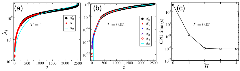
Figure 4: Comparison of the RG approach and direct diagonalization ($\Lambda_{0}$) for the 2D square lattice of size $50\times 50=2500$. (a) Direct diagonalization versus a single RG step at $T=1$. (b) Direct diagonalization versus four RG steps at $T=0.05$. (c) CPU time versus number of RG steps for $T=0.05$.

Similarly to the 1D case (Fig. 3), the RG approach performs poorly when $\gamma$ is not large, as is shown in panel (a). Panel (b) demonstrates the much better RG performance at a lower temperature, where the RG transformation has been applied four consecutive times. Numerical round-off errors are again seen as a vertical drop in the lower part of the direct diagonalization spectrum.

One can notice that at the same low temperature and number of nodes in the lattice, the 1D system [Fig. 3(c)] possesses a broader spectrum than the 2D one [Fig 4(b)]. The reason for this is that 1D diffusion is an exact lower boundary for $n$-dimensional diffusion, since hopping between any two distant nodes in $n$ dimensions can always be considered as hopping in 1D but along the “shortest” path, i.e., the path with highest rate constants.Bouchaud and Georges (1990)

The necessary condition for the coarse-graining procedure developed here to be valid is to have a clear separation of time-scales between intra- and inter-basin dynamics. Figs. 3 and 4 present a contradiction to this, since even at low temperature, where the RG procedure is seen to perform well, the eigenvalues from different coarse-graining levels [e.g., $\Lambda^{\prime}_{0}$, $\Lambda^{\prime}_{1}$, $\Lambda^{\prime}_{2}$ and $\Lambda^{\prime}_{3}$ in Fig. 4(b)] are seen to significantly overlap in magnitude. In fact, this observation does not contradict the previously mentioned condition, since the time-scale separation is only required for modes localized within the same small portion of the graph. An intra-basin relaxation mode within one portion of the large graph does not interact with an inter-basin hopping in some other distant portion of the graph. Therefore, the time-scale separation for these modes is not required for the RG procedure to work. Again, using the language of perturbation theory in quantum mechanics, one can say that for the hybridization of two interacting states to be weak, either the energy separation between the two states has to be large (i.e., large time-scale separation), or the interaction has to be weak. The latter condition resolves the apparent contradiction with overlapping time-scales in Figs. 3 and 4, since overlapping eigenvalues belong to intra- and inter-basin modes localized in different portions of the graph.

IV.3 Computational performance and scaling

As described above in detail, the RG procedure consists of splitting the entire graph into small basins, and then finding the intra-basin relaxation modes within each small basin. Splitting of the graph into basins requires a few consecutive scans of the entire graph, and the number of these scans is on the order of the average size of a basin, $n_{h}$, where $h$ specifies the current level of coarse-graining hierarchy. Thus, the computer time needed for the splitting of the graph can be estimated as $\sim n_{h}\times N_{h}$, where $N_{h}$ is the number of sites in the entire graph of hierarchy level $h$. Direct “brute-force” diagonalization of a matrix of size $m$ costs on the order of $m^{3}$, and since the number of basins is $\sim N_{h}/n_{h}$, the computational cost of diagonalization of all the basins within the graph is $\sim n^{3}_{h}\times N_{h}/n_{h}=n^{2}_{h}\times N_{h}$. Some additional minor computational overhead is present, but its cost is also growing linearly with the size of the graph, $N_{h}$. Since the average basin size does not depend on the size of the graph, the overall computational cost of the RG step is

$$t_{h}\sim N_{h},~{}~{}h=0,1,...,H-1,$$ (17)

where $N_{h}$ can be written as

$$N_{h}=\frac{N}{\prod^{h-1}_{h^{\prime}=0}n_{h^{\prime}}}\approx\frac{N}{n^{h}_{0}},$$ (18)

where $N\equiv N_{0}$ is the size of the initial microscopic graph. The last approximate equality is obtained assuming that the average size of basins is not too different at all the levels of hierarchy, so we take $n_{h}\approx n_{0}$. Summing up all the computational times for all the RG steps yields

$$t_{RG}=f(H)N,$$ (19)

where

$$f(H)\sim\sum^{H-1}_{h=0}1/n^{h}_{0}=\frac{n_{0}-n^{1-H}_{0}}{n_{0}-1}.$$ (20)

Thus, $f(H)$ is a slowly growing function of $H$ which rapidly converges to a constant value of $f(H\rightarrow\infty)\sim n_{0}/(n_{0}-1)$.

The direct diagonalization of the entire graph at the highest level of the hierarchy costs as

$$t_{H}\sim N^{3}_{H}=\left(\frac{N}{\prod_{h=0}^{H-1}n_{h}}\right)^{3}\approx\left(\frac{N}{n^{H}_{0}}\right)^{3}.$$ (21)

It is readily seen by comparing Eqs. (19) and (21) that if the original microscopic graph is large, then $t_{H}\gg t_{RG}$, since $t_{H}$ grows cubically with $N$. The overall computational time is thus dominated by $t_{H}$, and it decays exponentially with the number of hierarchy levels. However, since $t_{RG}$ grows and $t_{H}$ decays with $H$, it is expected that at a certain level of hierarchy, dependent on the size of the original graph, computational time becomes dominated by $t_{RG}$, which depends on $H$ only weakly.

Fig. 4(c) shows the overall computational time required to obtain the entire spectrum of hopping dynamics with $H=0,1,2,3$ or $4$ consecutive RG steps. The hierarchical RG procedure has been implemented into a Fortran 90 code, and all the calculations have been performed using a single core of an Intel(R) Xeon(R) CPU (2.66GHz). As is expected from the scaling considerations above, the direct diagonalization (i.e., $H=0$) is not only plagued by the numerical round-off errors at low temperatures, but is also very slow, since a single very large matrix has to be diagonalized. Each consecutive RG step reduces the computational cost exponentially. As predicted above, at sufficiently large hierarchy level the computational cost saturates, e.g., at $H=2$ for $N=2500$ in Fig. 4(c). It is also worth noting that since diagonalization of many small matrices (intra-basin relaxation) within each RG step is absolutely independent, the efficient parallelization of the code is possible, which can result in significant lowering of function $f(H)$ in Eq. (19) (not implemented in this work).

IV.4 Time-resolved luminescence

To illustrate how the developed RG approach can be used to evaluate spectroscopic observables, we simulate the time-resolved photoluminescence experiment for a system where an exciton migrates within an energy-disordered lattice. Specifically, we evaluate the time-resolved ensemble-average of photoluminescence energy. If an exciton is localized at node $i$ of energy $E_{i}$, it can recombine radiatively emitting a photon of energy $\hbar\omega=E_{i}$. Therefore, if we assume for simplicity that the rate of radiative recombination and its quantum yield do not depend on exciton energy, then the ensemble-average photoluminescence energy at time $t$ is given by $\langle E(t)\rangle=\langle E|p(t)\rangle$, i.e., by Eq. (6) for the average energy of an exciton.

The time-dependent ensemble-average energy of excitons within a 2D system of $50\times 50=2500$ nodes, measured relative to $\bar{E}$, is shown in Fig. 5.

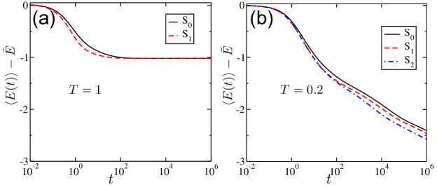
Figure 5: Time-resolved ensemble-averaged energy of an exciton for the 2D graph of $50^{2}=2500$ nodes. Temperature is set to $T=1$ (a) and $T=0.2$ (b).

For definiteness, all the nodes are assumed to be populated with equal probability at $t=0$, i.e., $|p_{0}\rangle=N^{-1}\sum_{i}|1)$. This initial state results in $\langle E(t)\rangle-\bar{E}=0$ at $t=0$ for both the exact solution obtained via direct diagonalization, $S_{0}$, as well as approximate RG-based ones, $S_{h}$ ($h>0$). At short times, the agreement between exact and approximate solutions is still good in panel (a), but at longer times ($t\sim 1-10$) the RG approach is inaccurate as expected for this high-temperature case, $T=1$. Within the same time domain, the agreement of the RG approach and the direct diagonalization is better in panel (b), where temperature is significantly lower ($T=0.2$), and, therefore, RG is expected to produce more accurate results. At large times the system is equilibrated in panel (a), so RG and direct diagonalization results coincide again. At lower temperatures, panel (b), the equilibration of the system is taking significantly longer and having not been reached at maximum observation time of $t=10^{6}$.

V Renormalization group flow

The analysis of dynamics of a system on different time- and length-scales, as well as interaction between these scales, can often be conveniently done by studying the RG flow – the evolution of system parameters (e.g., energy dispersion, rate constants) under consecutive RG transformations. A good example is the RG flow of the distribution of node energies. Fig. 6 shows the distribution of node energies for the original microscopic graph, $G_{0}$, as well as the energy distributions for graphs obtained from $G_{0}$ by consecutive RG transformations: $G_{1}$, $G_{2}$ and $G_{3}$.

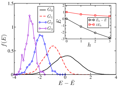
Figure 6: Energy distribution of nodes corresponding to hierarchy levels from $h=0$ (initial graph) to $h=3$ for the 2D system consisting of $200\times 200=40000$ nodes at $T=0.05$. The inset shows mean (black circles) and the standard deviation (red squares) corresponding to the distributions in the main figure. The size of the graphs for the each hierarchy level are 40000, 8046, 1123 and 142 for $G_{0}$, $G_{1}$, $G_{2}$ and $G_{3}$, respectively.

All energies are measured relative to $\bar{E}$, so the distribution of node energies for $G_{0}$ is just a Gaussian distribution (by construction) centered around $E=\bar{E}$ and with $\delta E=1$. Comparison of node energy distributions for $G_{0}$, $G_{1}$, $G_{2}$ and $G_{3}$ reveals the RG flow toward lower mean energies and lesser standard deviations, i.e., the distribution grows sharper under consecutive RG transformations. The extracted mean node energies and standard deviations are plotted by black circles and red squares, respectively, in the inset. The decrease of the mean node energy, $\bar{E}_{h}$, with $h$ can be easily understood from the fact that at very low temperatures energies of nodes of graph $G_{h}$ are essentially the energies of basin seeds of $G_{h-1}$, which are found by requiring each such point to be energetically lower than its immediate neighbors. This flow of $\bar{E}_{h}$ with $h$ is in fact reflected in Fig. 5 as the spectral diffusion – the decay of the ensemble-average photoluminescence energy with time. Indeed, the higher levels of the RG hierarchy correspond to longer observation times and, therefore, the dependence of average exciton energy on $h$ and on $t$ are expected to be similar.

The reduction of the standard deviation of node energies upon the RG step is less trivial and can be understood from the order statistics. Specifically, the mean and the standard deviation of a minimum of $n$ random variables, each sampled independently from the standard normal distribution, is given by (in the limit of $n\rightarrow\infty$) Serfling (2001)

$$\bar{E} =-\left(2\log n\right)^{1/2},$$

$$\delta E =\left(2\log n\right)^{-1/2},$$ (22)

As was mentioned above, at low temperatures, node energies of a graph obtained by the RG transformation are approximately equal to the energies of the seed nodes of the previous graph. In turn, each seed is found by identifying a node with minimum energy out of each immediate neighborhood. This procedure is very reminiscent of how a minimum value is found within each sample of size $n$ in the order statistics. Thus, we expect the mean node energy, $\bar{E}_{h}$, and the standard deviation, $\delta E_{h}$, to follow Eq. (22) with $n$ approximately given by the average size of the basin. Eq. (22) suggests the reduction of both mean and standard deviation of node energies upon the RG transformation, which is indeed in qualitative agreement with the numerical results (inset of Fig. 6). Quantitatively, the average basin size in the original graph is $n=\frac{N(G_{0})}{N(G_{1})}\approx 5$, so that Eq. (22) yields $\delta E_{1}\approx 0.56$ and $\bar{E}_{1}\approx-1.8$. The numerical results (from the inset) are $\delta E\approx 0.67$ and $\bar{E}\approx-1.2$, so the agreement is good considering the asymptotic ($n\rightarrow\infty$) nature of Eq. (22).

Fig. 7 schematically depicts the RG flow of $\gamma=\delta E/T$, i.e., how $\gamma$ changes when consecutive RG transformations are applied.

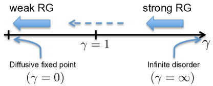
Figure 7: Schematic representation of the RG flow of $\gamma=\delta E/T$ in strong and weak disorder limits.

The RG approach developed in this work is valid only at $\gamma\gg 1$, as demonstrated above, and, therefore, one can call it strong-disorder RG. Fig. 6 and Eq. (22) suggest that upon consecutive RG transformations the value of $\gamma$ flows to lower magnitudes, as illustrated in Fig. 7. This imposes a natural restriction on the maximum number of accurate RG transformations, since above a certain number of transformations one has $\gamma\sim 1$, and the strong-disorder RG becomes inaccurate.

On the other hand, the weak disorder RG, discussed by Deem and Chandler,Deem and Chandler (1994) demonstrates the same direction of the flow, i.e., reduction of $\gamma$ upon each consecutive RG step at $\gamma\ll 1$. In fact, the weak RG flow in this domain ultimately converges to the stable fixed point at $\gamma=0$, which is the pure diffusion. Neither of these RG approaches is valid in the intermediate disorder regime, $\gamma\sim 1$. However, the exact solution for the 1D model suggests that the long-time behavior of 1D model at arbitrarily strong gaussian disorder is always purely diffusive.Bouchaud and Georges (1990); Deem and Chandler (1994) Furthermore, the long-time hopping dynamics in 1D model is an exact lower boundary for models with higher dimensionality.Bouchaud and Georges (1990) Therefore, observing hopping in a model with gaussian energy disorder at increasing length- or time-scale is expected to always correspond to a decreasing effective disorder. We therefore put a dotted arrow in Fig. 7 to reflect the expected flow direction at $\gamma\sim 1$, even though we are not aware of any RG approach valid in this region.

Finally, we briefly discuss the RG flow of the distribution of the pre-exponential factors of rate constants. Pre-exponential factors are all degenerate (i.e., the same) within the classical MA model. However, it is quite obvious that even if this degeneracy is present in $G_{0}$, the pre-exponential factors of the rate constants of $G_{1}$ will have a certain finite dispersion since pre-exponential factors of inter-basin rate constants are determined by activation barriers of hopping between basins, and the heights of these activation barriers are random variables themselves. Thus, it is expected that the degeneracy of the pre-exponential factors (i.e., their non-randomness) is irrelevant in the RG sense, i.e., the system flows away from this degeneracy upon consecutive RG transformations. To illustrate this, we compare the spectra of eigenvalues for the modified and classical MA models, the latter obtained from the modified one by setting the activation energy to a certain fixed non-random value. Fig. 8 shows these spectra ($S_{2}$ at $T=0.05$ for the 2D lattice with 2500 nodes) for the modified MA model (black line) with $\epsilon_{ij}^{a}$ sampled uniformly within $(0,1)$ interval, as well as for the classical MA model with the activation energy set to $\epsilon_{ij}^{a}=1$ (magenta diamonds), $\epsilon_{ij}^{a}=0.6$ (red circles) and $\epsilon_{ij}^{a}=0$ (blue squares).

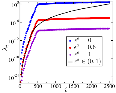
Figure 8: The eigenspectrum for the modified MA model ($\epsilon_{ij}^{a}\rightarrow\mathcal{U}(0,1)$, black line), as well as for the classical MA model with the fixed pre-exponential factor obtained from Eq. (16) by fixing the activation energy: $\epsilon_{ij}^{a}=0$ (blue squares), $\epsilon_{ij}^{a}=0.6$ (red circles) and $\epsilon_{ij}^{a}=1$ (magenta diamonds). All the eigenspectra are evaluated for the 2D system with 2500 nodes at $T=0.05$ applying two consecutive RG steps.

It is seen that in the high-$\lambda$ part of the spectrum, the modified and classical MA models produce qualitatively different results. Specifically, the classical MA model produces an almost flat spectrum due to the high degree of degeneracy of eigenvalues. However, the lower part of the spectrum is qualitatively the same for the two models, except for a vertical shift. The origin of this shift is clear since, e.g., at $\epsilon_{ij}^{a}=1$ all the rate constants are lower than those for the activation energy uniformly distributed between $0$ and $1$. Therefore, the spectrum with this fixed activation energy is expected to be generally lower than the one with finite dispersion of activation energies (compare the black line and magenta diamonds in Fig. 8). A similar argument explains why the eigenspectrum with $\epsilon_{ij}^{a}=0$ is generally higher than the one with the dispersion of pre-exponential factors present (compare the black line and blue squares in Fig. 8) In fact, it is possible to numerically find the fixed activation energy, $\epsilon_{ij}^{a}=0.6$, at which the lower portion of the eigenspectra of the standard and modified MA models practically coincide. Therefore, the degeneracy, or non-randomness, of the pre-exponential factors is irrelevant in the RG sense, which is exactly the reason why we adopted the modified MA model from the onset.

VI Conclusion

In this paper, we formulate and computationally implement a numerical real-space RG approach to study the hopping dynamics on energy-disordered lattices at low temperature. Our approach is similar to methods developed in Refs. Dasgupta and Ma, 1980; Iglói and Monthus, 2005; Lee et al., 2009; Amir, Oreg, and Imry, 2010, which were originally introduced to treat disordered Ising-type models. This similarity stems from the fact that in both cases fast degrees of freedom can be treated independently from slow ones, giving rise to renormalization of the latter. However, we emphasize that in this work the fast degrees of freedom are not actually “integrated out”, since the entire spectrum is recovered, not just its low-energy portion. The other difference of the approach, developed in this work, from that in Refs. Dasgupta and Ma, 1980; Iglói and Monthus, 2005; Lee et al., 2009; Amir, Oreg, and Imry, 2010 is that the former is dynamical in a sense that the dynamics in the form of eigenvalues and eigenvectors of relaxation modes is recovered at all timescales, and not just equilibrium properties of a system of interest.

In this work, the developed RG approach is applied to discrete systems, represented by graphs. In fact, in the case of strong disorder the approach can be straightforwardly applied to continuous systems. Indeed, even if the microscopic system is initially continuous, the population trapping in local minima leads to the appearance of the discrete-like dynamics, i.e., hopping between potential minima of the continuous landscape. In other words, an RG transformation can still be introduced, and its first application to the continuous system in the regime of strong disorder immediately leads to hopping on a graph. Thus, the continuity of a system is irrelevant in the RG sense in the case of strong disorder. Interestingly, it is exactly the opposite in the weak disorder limit, where discreteness becomes irrelevant and continuity finally “sets in” leading to pure diffusion at large timescales.

We expect the developed approach to become useful in studying hopping dynamics in various systems of practical interest including polymer films and nanoparticle aggregates. A combination of this method with the weak-disorder RG groupBouchaud and Georges (1990); Deem and Chandler (1994) might become especially fruitful. Indeed, as was discussed above, the validity range of strong-disorder RG is limited by the fact that the system“flows away” from strong disorder upon consecutive RG transformations. However, once the disorder is not strong, the weak-disorder approach can be applied (at least approximately), ultimately leading to the pure diffusion fixed point (see Fig. 6). Therefore, the combination of the strong-disorder RG method developed in this work with the weak-disorder RG approach might yield a universal methodology capable of treating hopping dynamics in systems with an arbitrary strength of disorder. Furthermore, since the attractive RG fixed point – pure diffusion – possesses an elementary analytical solution, the universal methodology can be applied to systems of infinite extent, yielding the large-scale diffusion coefficient, determined by small-scale hopping rate constants.Bouchaud and Georges (1990)

K.A.V. is thankful to Y. Dubi, A. Zhugayevych and J. Bjorgaard for useful discussions and comments on the manuscript. Los Alamos National Laboratory, an affirmative action equal opportunity employer, is operated by Los Alamos National Security, LLC, for the National Nuclear Security Administration of the U.S. Department of Energy under contract DE-AC52-06NA25396. V.Y.C acknowledges support by the National Science Foundation under Grant No. CHE-1111350.

References

- Dill and MacCallum (2012) K. A. Dill and J. L. MacCallum, Science 338, 1042 (2012).
- Levi et al. (2011) L. Levi, M. Rrechtsman, B. Freedman, T. Schwartz, O. Manela, and M. Segev, Science 332, 1541 (2011).
- Lee et al. (2006) K. Lee, S. Cho, S. H. Park, A. J. Heeger, C.-W. Lee, and S.-H. Lee, Nature 441, 65 (2006).
- Nicolai et al. (2012) H. T. Nicolai, M. . Kuik, G. A. H. Wetzelaer, B. de Boer, C. Campbell, C. Risko, J. L. Brédas, and P. W. M. Blom, Nature Mat. 11, 882 (2012).
- Hermosa et al. (2013) C. Hermosa, J. V. Álvares, M.-R. Azani, C. J. Gómez-García, M. Fritz, J. M. Soler, J. Gómez-Herrero, C. Gómez-Navarro, and F. Zamora, Nature Commun. 4, 1 (2013).
- Arkhipov, Emelianova, and Bässler (2004) V. I. Arkhipov, E. V. Emelianova, and H. Bässler, Phys. Rev. B 70, 205205 (2004).
- Ahn, Wright, and Bardeen (2007) T.-S. Ahn, N. Wright, and C. Bardeen, Chem. Phys. Lett. 446, 43 (2007).
- Athanasopoulos et al. (2008) S. Athanasopoulos, E. Hennebicq, D. Beljonne, and A. Walker, J. Phys. Chem. C 112, 11532 (2008).
- Köhler and Bässler (2011) A. Köhler and H. Bässler, J. Mat. Chem. 21, 4003 (2011).
- Hwang and Scholes (2011) I. Hwang and G. Scholes, Chem. Mater 23, 610 (2011).
- Meskers et al. (2001) S. C. J. Meskers, J. Hübner, M. Oestreich, and H. Bässler, J. Phys. Chem. B 105, 9139 (2001).
- Förster (1948) T. Förster, Ann. Phys. (NY) 2, 55 (1948).
- Dexter (1953) D. L. Dexter, J. Chem. Phys. 21, 836 (1953).
- J. L. Mohanan (2005) S. L. B. J. L. Mohanan, I. U. Arachchige, Science 307, 397 (2005).
- Gaponik, Herrmann, and Eychmuller (2012) N. Gaponik, A. K. Herrmann, and A. Eychmuller, Phys. Chem. Lett. 3, 8 (2012).
- Crooker et al. (2002) S. A. Crooker, J. A. Hollingsworth, S. Tretiak, and V. I. Klimov, Phys. Rev. Lett. 89, 186802 (2002).
- Reitinger et al. (2011) N. Reitinger, A. Hohenau, S. Köstler, J. R. Krenn, and A. Leitner, Phys. Status Solidi A 208, 710 (2011).
- Belyakov and Burdov (2011) V. A. Belyakov and V. A. Burdov, J. Comput. Theor. Nanosci. 8, 365 (2011).
- Ganguly and Brock (2011) S. Ganguly and S. L. Brock, J. Mat. Chem. 21, 8800 (2011).
- De Freitas et al. (2012) J. N. De Freitas, L. Korala, L. X. Reynolds, S. A. Haque, S. L. Brock, and A. F. Nogueira, Phys. Chem. Chem. Phys. 14, 15180 (2012).
- Deem and Chandler (1994) M. W. Deem and D. Chandler, J. Stat. Phys. 76, 911 (1994).
- Bouchaud and Georges (1990) J. P. Bouchaud and A. Georges, Phys. Rep. 195, 127 (1990).
- Note (1) This corresponds to the case where the configuration space of the system is discrete (because the set of nodes of the graph is countable). In Sec. VI we briefly discuss how the proposed RG method can also be applied in the continuous case.
- van Kampen (1992) N. G. van Kampen, Stochastic Processes in Physics and Chemistry (North-Holland, Amsterdam, 1992).
- Note (2) A generic non-symmetric matrix is not necessary diagonalizable, but is due to the detailed balance and population conservation constraints imposed.van Kampen (1992).
- Hänggi, Talkner, and Borkovec (1990) P. Hänggi, P. Talkner, and M. Borkovec, Rev. Mod. Phys. 62, 251 (1990).
- Miller and Abrahams (1960) A. Miller and E. Abrahams, Phys. Rev. 120, 745 (1960).
- Serfling (2001) R. Serfling, Approximation Theorems of Mathematical Statistics, Wiley Series in Probability and Statistics (John Wiley & Sons, 2001).
- Dasgupta and Ma (1980) C. Dasgupta and S.-K. Ma, Phys. Rev. B 22, 1305 (1980).
- Iglói and Monthus (2005) F. Iglói and C. Monthus, Phys. Rep. 412, 277 (2005).
- Lee et al. (2009) T. E. Lee, G. Refael, M. C. Cross, O. Kogan, and J. L. Rogers, Phys. Rev. E 80, 046210 (2009).
- Amir, Oreg, and Imry (2010) A. Amir, Y. Oreg, and Y. Imry, Phys. Rev. Lett. 105, 070601 (2010).