Loschmidt echo and the many-body orthogonality catastrophe in a qubit-coupled Luttinger liquid

Abstract

We investigate the many-body generalization of the orthogonality catastrophe by studying the generalized Loschmidt echo of Luttinger liquids (LLs) after a global change of interaction. It decays exponentially with system size and exhibits universal behaviour: the steady state exponent after quenching back and forth $n$-times between 2 LLs (bang-bang protocol) is $2n$-times bigger than that of the adiabatic overlap, and depends only on the initial and final LL parameters. These are corroborated numerically by matrix-product state based methods of the XXZ Heisenberg model. An experimental setup consisting of a hybrid system containing cold atoms and a flux qubit coupled to a Feshbach resonance is proposed to measure the Loschmidt echo using rf spectroscopy or Ramsey interferometry.

Introduction. The long coherence times and the possibility to control parameters very accurately in optical lattices allow to simulate exciting non-equilibrium effects in quantum many body systems. Particular attention has been devoted to the evolution of quantum stated after quenchespolkovnikovrmp in which a parameter in the Hamiltonian is changed either suddenly or gradually. By measuring the Loschmidt echo (LE), it is possible to get insight into the dynamical properties of the quantum-many body state.

The LE is defined as the overlap of two wave functions, $|\Psi_{0}(t)\rangle$ and $|\Psi(t)\rangle$, evolved from the same initial state, but with different Hamiltonians, $H_{0}$ and $H$,

$$\mathcal{L}(t)\equiv\left|\langle\Psi_{0}(t)|\Psi(t)\rangle\right|^{2}.$$ (1)

It measures the ”distance” between two quantum states and serves to quantify irreversibility and chaos in quantum mechanicsperes ; physrep ; goussev . Furthermore, it can be used to diagnose quantum phase transitionspollmann , and is also an important quantity in various fields of physics, ranging from nuclear magnetic resonance to quantum computation and information theory. For the latter, the LE is of utmost importance since it measures how small changes during a time evolution cause decoherence and are detrimental for quantum information processing and storage.

While the theoretical concept behind the LE is very clear, experimental protocols to measure the overlap of two wave functions, are challenging and rare. Experimentally, the LE and the closely related fidelity has only been observed in systems with limited degrees of freedom zhang2 , by coupling the system of interest to a single qubit, whose states probe the wavefunction of the system at different values of some external parameters. Also, while the LE for local perturbations – the X-ray edge singularity problem – is well understood, its behavior in generic many-body systems is poorly described venuti2 . Studies so far mostly focused on local perturbations and simple refermionizable spin chain modelsgoold ; knap ; rossini .

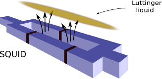
Figure 1: (Color online) Schematics of the experimental setup. The black segments on the SQUID denote the Josephson junctions, the arrows stand for the total magnetic field. By changing the eigenstate of the flux qubit, the total flux hence the total magnetic field changes, controlling the Feshbach resonance in the cold atomic LL.

Here we study the interaction driven LE of a genuine interacting one-dimensional system, a Luttinger liquid (LL). One-dimensional strongly correlated systems often form such Luttinger liquids (LL), and can also be created from cold atoms cazalillarmp . Recently, the LL wavefunction has been used to evaluate the overlap of distinct LL ground states fjaerestad ; yang , and optimal protocols producing maximal overlaps with reference states have also been investigated rahmani . In this work, we evaluate the LE within the Luttinger liquid (LL) description for a time dependent Hamiltonian, and verify the predictions of the LL model numerically on the XXZ Heisenberg chain using matrix-product state (MPS) based methods. Furthermore, we propose an experimental setup to measure the LE of a Luttinger liquid, where a flux qubit coupled to a Feshbach resonance is used to control the interaction in one-dimensional cold atom gas (see Fig. 1).

Model. A LL can be described in terms of bosonic sound-like collective excitations, regardless to the statistics of the original system. The LL Hamiltonian is given bygiamarchi

$$H_{0}=\sum_{q\neq 0}\left(\omega_{q}a_{q}^{+}a_{q}+\frac{g_{i}(q)}{2}[a_{q}a_{-q}+a_{q}^{+}a_{-q}^{+}]\right)\;,$$ (2)

where $g_{i}(q)$ is the initial interaction, and $\omega_{q}$ the energy of bosonic excitations. In the following, we shall assume that $H=H(t)$ has the same form as Eq. (2), but with a time dependent coupling,

$$g_{q}\to g_{q}(t)=g_{i}({q})+\Delta g_{q}(t),$$ (3)

where $\Delta g_{q}(t)=[g_{i}({q})-g_{f}({q})]Q(t)$, and $g_{f}({q})$ is the final interaction strength. For a conventional LE $Q(t)\equiv 1$ for $t>0$, but here we allow any time dependence, and only assume that $Q(0)=0$ and $Q(t)=1$ after some ”transition time” $\tau$  .

The Hamiltonian $H(t)$ is quadratic, and can be diagonalized at any instance. Its initial and final quasiparticle spectra are simply given by $\omega_{i/f}({q})=(\omega^{2}_{q}-g_{i/f}^{2}({q}))^{1/2}$, and the strength of interaction in these states is conveniently characterized by the dimensionless LL parameters, $K_{i/f}=\sqrt{\left[{\omega_{q}-g_{i/f}({q})}\right]/\left[{\omega_{q}+g_{i/f}({q})}\right]}$.

To compute the LE, it is convenient to first diagonalize Eq. (2) by a standard, time independent Bogoliubov transformation, yielding $H_{0}=\sum_{q\neq 0}\omega_{i}({q})\;b_{q}^{+}b_{q}$ up to a constant shift of energy. In this basis, $H(t)$ reads

$$H=\sum_{q\neq 0}\omega(q,t)b_{q}^{+}b_{q}+\frac{g(q,t)}{2}[b_{q}b_{-q}+b_{q}^{+}b_{-q}^{+}]+\dots$$ (4)

with $\omega(q,t)=\omega_{i}({q})-\Delta g_{q}(t)\frac{g_{i}({q})}{\omega_{i}({q})}$ and $g(q,t)={\Delta g_{q}(t)}\frac{\omega_{q}}{\omega_{i}({q})}$, and the dots stand for an unimportant time dependent energy shift. We emphasize that our setting is very general  , and equally applies for a spinless fermion, boson or spin systemgiamarchi .

Analytical results. In order to calculate the LEsilva , we need to determine the wave function of our quenched LL. This can be achieved by realizing that Eq. (4) couples only pairs of states with $q$ and $-q$. Consequently, the total time-evolution operator is the product of the separate evolution operators $U_{q}(t)$ for all $q$’s. Finding $U_{q}(t)$ for a given pair of modes can be accomplished by realizing that the operators appearing in the Hamiltonian, $K_{0}(q)=(b^{+}_{q}b_{q}+b_{-q}b^{+}_{-q})/{2}$, $K_{+}(q)=b^{+}_{q}b^{+}_{-q}$ and $K_{-}(q)=b_{q}b_{-q}$ are the generators of SU(1,1) Lie algebra. Generalizing the results of squeeze operators to the present case, and exploiting a faithful matrix representation of the SU(1,1) generators  gilmore , the time evolution operator $U_{q}(t)$ can finally be expressed as EPAPS

$$U_{q}(t)=\exp[C_{+}(q,t)K_{+}(q)]\exp[C_{0}(q,t)K_{0}(q)]\times$$

$$\times\exp[C_{-}(q,t)K_{-}(q)+i\varphi_{q}(t)].$$ (5)

Here $\varphi_{q}(t)$ is an unimportant phase, and the coefficients $C_{0}(q,t)$ and $C_{\pm}(q,t)$ can be expressed in terms of the time dependent Bogoliubov coefficients, $u_{q}(t)$ and $v_{q}(t)$,

$$C_{+}(q,t)={v_{q}^{*}(t)}/{u_{q}^{*}(t)},\hskip 5.69054ptC_{-}(q,t)=-{v_{q}(t)}/{u_{q}^{*}(t)},$$ (6a)

$$C_{0}(q,t)=-2\ln(u_{q}^{*}(t)),$$ (6b)

with the coefficients $u_{q}(t)$ and $v_{q}(t)$ satisfying EPAPS

$$i\partial_{t}\left[\begin{array}[]{c}u_{q}(t)\\ v_{q}(t)\end{array}\right]=\left[\begin{array}[]{cc}\omega(q,t)&g(q,t)\\ -g(q,t)&-\omega(q,t)\end{array}\right]\left[\begin{array}[]{c}u_{q}(t)\\ v_{q}(t)\end{array}\right]$$ (13)

with $[u_{q}(0),v_{q}(0)]=[1,0]$. We can now express the time evolution of any initial state $|\Psi_{0}\rangle$ as $|\Psi(t)\rangle=U(t)|\Psi_{0}\rangle$, with $U(t)=\prod_{q>0}U_{q}(t)$.

In the following, for simplicity, we take $|\Psi_{0}\rangle$ as the ground state wavefunction of $H_{0}$, which is the vacuum for the $b$ bosons. Then the time evolved, normalized wave function simplifies to

$$|\Psi(t)\rangle=e^{-i\Phi(t)+\sum_{q>0}\bigl{[}\frac{v_{q}^{*}(t)}{u_{q}^{*}(t)}b^{+}_{q}b^{+}_{-q}-\ln[u_{q}^{*}(t)]\bigr{]}\vphantom{\sum_{i}}}|\Psi_{0}\rangle,$$ (14)

with $\Phi(t)$ an overall phase factor. This generalizes the equilibrium resultsfjaerestad ; yang to the non-equilibrium situation, encoded via the time dependent Bogoliubov coefficients. Then the time evolution under the action of $H_{0}$ is trivial, since $|\Psi_{0}\rangle$ only picks up a phase, and the LE takes a particularly simple form

$$\mathcal{L}(t)=\exp\left(-\sum_{q>0}\ln\left(|u_{q}(t)|^{2}\right)\right).$$ (15)

This result, in combination with Eq. (13) determines the complete time dependence of the generalized LE in a LL. It holds true for any non-equilibrium evolution, and expresses the LE solely in terms of the number of excited quasiparticles in the final state. We regularize the $q$ sums in (15) by an $\exp(-\alpha|q|)$ factor, with $1/\alpha$ an ultraviolet cutoffgiamarchi .

We can now use the function $Q(t)$ to calculate the LE. Changing $Q(t)$ adiabatically, one obtains from Eq. (13) $|u^{\rm ad}_{q}(t)|^{2}=1/2+\left({K_{i}}/{K_{f}}+{K_{f}}/{K_{i}}\right)/4$ for times $t>\tau$. The LE is in this case just the overlap of the ground states of the initial and final Hamiltonian and, in agreement with Refs. fjaerestad ; yang , reads as

$$\mathcal{L}_{ad}=\left(\frac{1}{2}+\frac{1}{4}\left(\frac{K_{i}}{K_{f}}+\frac{K_{f}}{K_{i}}\right)\right)^{-L/2\pi\alpha},$$ (16)

with $L$ being the system size. This remains valid in the steady state for near-adiabatic quenches, $\tau\gg\alpha/v$ with $v$ being the sound velocity in the final state.

For $Q(t>0)=1$, i.e., a conventional ”sudden quench” (SQ) cazalillaprl LE, however, Eq. (13) yields

$$|u_{q}(t)|^{2}=1+\frac{1}{4}\sin^{2}(\omega_{f}({q})t)\left(\frac{K_{f}}{K_{i}}-\frac{K_{i}}{K_{f}}\right)^{2},$$ (17)

with $\omega_{f}(q)=v|q|$ denoting the excitation energy after the quench. By plugging this back to Eq. (15), we find for the short time limit ($t\ll\alpha/v$)

$$\mathcal{L}_{SQ}(t)\sim\exp\left(-c\;L\;(t/t_{c})^{2}/\alpha\right)$$ (18)

where $c$ is a non-universal constant of order unity. The characteristic decay time of this expression is $t_{c}\equiv 4\alpha/v|K_{f}/K_{i}-K_{i}/K_{f}|$, and $1/t_{c}^{2}\sim$ can be identified as the variance of energy per particle after the quench per particle. For intermediate times $t\sim t_{c}$, the LE displays a non-universal transient signal (see Fig. 2b), however, for very long times, $t\gg\alpha/v$, the LE for SQ becomes time independent and universal:

$$\mathcal{L}_{SQ}(t\gg\alpha/v)=\left(\frac{1}{2}+\frac{1}{4}\left(\frac{K_{i}}{K_{f}}+\frac{K_{f}}{K_{i}}\right)\right)^{-L/\pi\alpha},$$ (19)

which holds also true for fast quenches, $\tau\ll\alpha/v$. Excitations are only produced at $t=0$, which interfere with each other for a short amount of time, causing Eq. (18), but after this phase coherence is lost, excitations propagate independently and only their total number determines the overlap.

By Eq. (16) we just established that for $t\to\infty$

$$\mathcal{L}_{SQ}=\mathcal{L}_{ad}^{2}.$$ (20)

This can be understood in terms of simple physical arguments and must hold in general, toorossini : the adiabatic LE measures just the square of the overlap $\langle G|G_{0}\rangle$ of the ground state of the initial and final Hamiltonians, which is the probability weight of the ground state of $H$ in $|G_{0}\rangle=|\Phi_{0}\rangle$. For a regular LE, $\langle\Phi(t)|\Phi_{0}(t)\rangle=\langle\Phi_{0}|e^{itH}e^{-itH_{0}}|\Phi_{0}\rangle$. Inserting here the complete set of eigenstates of $H$ between the two propagators, the excited states amount in oscillating terms, interfering destructively, and only the ground state contribution remains, yielding asymptotically in the thermodynamic limit $|\langle\Phi(t)|\Phi_{0}(t)\rangle|=|\langle G|G_{0}\rangle|^{2}$, and thus $\mathcal{L}_{SQ}(t)=|\langle\Phi(t)|\Phi_{0}(t)\rangle|^{2}\xrightarrow{t\rightarrow\infty}|\langle G|G_{0}\rangle|^{4}=\mathcal{L}_{ad}^{2}$ . Using the analogy to work statisticssilva , this is the square of the probability to stay in the ground state after the quench.

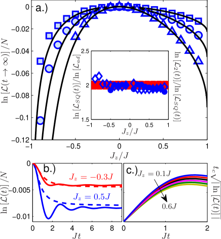
Figure 2: (Color online) a.) The exponent of the generalized Loschmidt echo is shown for SQ $n=1$ (circle), double quench $n=2$ (triangle) and adiabatic time evolution (square) for the XXZ Heisenberg model in the steady state, starting from the XX point and ending up at a finite $J_{z}$, obtained numerically from MPS based methods (when convergence was reached). The solid lines are the analytical results from Eqs. (16) and (19). The inset shows the ratio of the SQ and adiabatic exponents (diamond) and the $n=2$ and 1 exponents (circle) from numerics, which agrees well with the theoretically expected value of 2. b.) Typical numerical results (solid lines) of the LE of the XXZ model are shown for a SQ from the XX point to $J_{z}=0.5J$ and -0.3$J$, the dashed curve is the analytical expression using Eqs. (15) and (17). c.) The scaling of the numerical data expected from Eq. (18) for short times for a SQ is visualized from $J_{z}=0$ to $0.1J$ to $0.6J$ with $0.1J$ steps from top to bottom in arbitrary units.

The exponent of the LE is further enhancedEPAPS by repeating the $Q(t>0)$: SQ to 1, holding time $t$, SQ to 0, holding time $t$ sequence $n$ times (bang-bang protocol). The generalized LE is the $n$th power of the SQ overlap in Eq. (19) as $\mathcal{L}_{n}(2nt)=\mathcal{L}_{SQ}^{n}(t)=\mathcal{L}_{ad}^{2n}$ in the post-quench steady state, therefore the exponent is enhanced by a factor of $n$.

Numerics. We tested the analytical predictions numerically on the one-dimensional XXZ Heisenberg modelgiamarchi , covering $1/2<K<\infty$, for adiabatic ramps and SQ from $J_{z}=0$ to a finite $J_{z}$. We performed the simulations using a combination of MPS Fannes-1992 based infinite density matrix renormalization group White-1992 ; Kjaell-2012 ; McCulloch-2008 to find the ground state variationally, and the infinite time evolving block decimation Vidal-2007 algorithms to simulate the quench. The LE is calculated by finding the dominant eigenvalue of a ”generalized” transfer matrix which we obtain by contracting the tensors representing the two states.

The factor $L/\pi\alpha$ in the exponent in Eqs. (16) and (19) contains the unknown short distance cutoff. However, its value can be fixed by calculating the fidelity susceptibility, $\chi_{f}$, around the non-interacting XX point of the Heisenberg model, in which case $L/2\pi\alpha\approx N\chi_{f}\pi^{2}$, where $N$ is the number of lattice sites and $\chi_{f}\approx 0.0195$sirker . Using then the Bethe Ansatz result giamarchi , $K=\pi/2[\pi-\arccos(J_{z}/J)]$, we find an excellent agreement with the numerical data with no fitting parameter (see Fig. 2a). This excellent agreement is somewhat surprising since, as expected, the non-universal transient signals clearly differ in the LL approach and the numerics, and also, because the LL description completely neglects (asymptotically irrelevant) back scattering processes, contained in the the lattice calculations.

Slight deviations show up only at the end points of the critical region of the XXZ Heisenberg model in Fig. 2. Close to the $J_{z}=J$ point, the previously mentioned back scattering term, driving the Kosterlitz-Thouless phase transition causes a slight disagreement. Upon approaching the ferromagnetic critical point at $J_{z}=-J$, on the other hand, the validity of bosonization shrinks to very small energies, and the high energy modes, absent in the present considerations, also influence the overlap.

Detection: We propose to measure the LE of the LL in a cold atomic setting, where a flux qubitfriedman ; vanderWal is used to control the interaction between a the atoms. Though here we focus on a one dimensional LL, the proposed setup also opens up the possibility to study the LE in higher dimensional interacting systems. The flux qubit consists of a Josephson junction circuit, and is governed by the Hamiltonian $H_{\rm qubit}=\epsilon\sigma_{z}+\Delta\sigma_{x}$, with $\Delta$ the tunneling between the two eigenstates of $\sigma_{z}$, $|\circlearrowleft\rangle$ and $|\circlearrowright\rangle$, carrying oppositely circulating persistent currents, $\pm I$, and $\epsilon$ the energy splitting. In addition to the external flux, $\Phi_{\rm ext}$, the states $|\circlearrowleft\rangle$ and $|\circlearrowright\rangle$ generate an additional flux, $\Phi_{f}$. Ideally, tunneling between them is suppressed. The one-dimensional quantum gas is prepared in a two-dimensional optical lattice potentialGreiner2001 at the chip surface, hosting the flux qubit. A few microns thick, high reflectivity ($>$99.9%) dielectric coating of the chip (not shown in Fig. 1) can shield the superconducting device from the laser power (mW) incident during the measurement time (ms). The quantum gas is positioned at the flux qubit (see Fig. 1) by positioning the laser beams (optical tweezers), such that the total magnetic field of the state $|\circlearrowright\rangle$ of flux $\Phi_{\rm ext}+\Phi_{f}$ be at a Feshbach resonance, while the field of the state $|\circlearrowleft\rangle$ of flux $\Phi_{ext}-\Phi_{f}$, be further away from the resonance. We estimated the qubit switching-induced magnetic field difference for an elongated rectangular flux qubit, with parallel sides comparable to the length of a typical cold atomic tube ($\sim 10~{}\mu$m). Assuming a persistent current of $I=2\mu$A and a separation of $d=2R=2\mu$m between the two lines of the qubit, we obtain a field difference $\delta B_{f}\sim 16$ mG. Although relatively small, this field is comparable to the width $\Delta B=15~{}$mG of some narrow Feshbach resonances used to realize a LL in ⁸⁷Rb systems widera .

In this setup, one could use rf spectroscopy and measure the absorption spectrum of the qubit Pothier in the presence and in the absence of the trapped gas. Similar to the X-ray edge singularity problem, this absorption signal is just proportional to the Fourier transform of the LE. In this case, the qubit can be positioned far away from the degeneracy point, at $|\epsilon|\gg\Delta$, and the rf/mw spectroscopy can be referenced to high stability quartz oscillators ($\delta f/f\sim 10^{-13}$) to resolve the fine structure at the absorption edge.

Alternatively, the LE can be measured using Ramsey interferometryknap ; goold : initializing the qubit in the $|\circlearrowleft\rangle$ state with weak interactions to the cold atoms, yields a wavefunction $|\circlearrowleft\rangle\otimes|\Psi_{0}\rangle$ at $t=0$. By applying a $\pi/2$ rf pulse , a superposition of the two qubit states is produced $(|\circlearrowleft\rangle+|\circlearrowright\rangle)/\sqrt{2}\otimes|\Psi_{0}\rangle$, yielding distinct, qubit state dependent time evolution for $|\Psi_{0}\rangle$. After time $t$, a second $\pi/2$ pulse and the measurement of the qubit current $\langle\hat{I}\rangle\sim\langle\sigma_{z}\rangle$ is performed, giving a signal proportional to ${\cal L}(t)$. The timescale separating Eqs. (19) and (18) is estimated as $\alpha/v\sim 40~{}\mu$s from a typical Fermi temperature of 1 $\mu$K or trapping frequency of $25$ kHzwidera , and $t_{c}$ can be made even shorter by executing large quenches. Given the rapid progress of technology of flux qubitsnorirmp , these are already accessible with current coherence times and will be even more so in the future.

Note added. After accomplishing this work, we became aware of related proposals to measure the work statistics in hybrid architecturesmazzola ; dorner .

I Supplementary material for ”Loschmidt echo and the many-body orthogonality catastrophe in a qubit-coupled Luttinger liquid”

II Derivation of the time evolution operator

The time evolution operator of a given mode is

$$U_{q}(t)=\exp[C_{+}(q,t)K_{+}(q)]\exp[C_{0}(q,t)K_{0}(q)]\times$$

$$\times\exp[C_{-}(q,t)K_{-}(q)+i\varphi_{q}(t)],$$ (S1)

where the operators

$$K_{0}(q)=\frac{b^{+}_{q}b_{q}+b_{-q}b^{+}_{-q}}{2},$$ (S2)

$$K_{+}(q)=b^{+}_{q}b^{+}_{-q},\hskip 22.76219ptK_{-}(q)=b_{q}b_{-q}$$ (S3)

are the generators of a SU(1,1) Lie algebra, satisfying $[K_{+}(q),K_{-}(q)]=-2K_{0}(q)$, $[K_{0}(q),K_{\pm}(q)]=\pm K_{\pm}(q)$, and the operators for distinct $q$’s commute with each other.

Using these and a faithful matrix representation of the generators of SU(1,1) gilmore , the coefficients in Eq. (S1) of a given mode are determined from substituting this to the Schrödinger equation of the time evolution operator, $i\dot{U}(t)=HU(t)$, or rather $i\dot{U}(t)U^{*}(t)=H$, where $\dot{U}(t)=\partial_{t}U(t)$. Using the SU(1,1) commutation relations, we derive the identities

$$\exp(aK_{+})K_{0}=(K_{0}-aK_{+})\exp(aK_{+}),$$ (S4)

$$\exp(bK_{0})K_{-}=K_{-}\exp(bK_{0}-b),$$ (S5)

$$\exp(aK_{+})K_{-}=(K_{-}+a^{2}K_{+}-2aK_{0})\exp(aK_{+}).$$ (S6)

Using these, we finally get

$$-\dot{C}_{+}(q,t)+C_{+}(q,t)\dot{C}_{0}(q,t)-$$

$$-\exp[-C_{0}(q,t)]C_{+}^{2}(q,t)\dot{C}_{-}(q,t)=ig(q,t),$$ (S7)

$$i\dot{C}_{-}(q,t)\exp[-C_{0}(q,t)]=g(q,t),$$ (S8)

$$-\dot{C}_{0}(q,t)+2C_{+}(q,t)\exp[-C_{0}(q,t)]\dot{C}_{-}(q,t)=2i\omega(q,t),$$ (S9)

$$\dot{\varphi}_{q}(t)=\omega(q,t),$$ (S10)

with initial conditions $C_{+}(q,0)=C_{0}(q,0)=C_{-}(q,0)=\varphi_{q}(0)=0$. These can be solved following Ref. truax as

$$C_{+}(q,t)=\frac{v^{*}(q,t)}{u^{*}(q,t)},\hskip 11.38109ptC_{-}(q,t)=-\frac{v(q,t)}{u^{*}(q,t)}$$ (S11)

$$C_{0}(q,t)=-2\ln(u^{*}(q,t)),\hskip 5.69054pt\varphi_{q}(t)=\int\limits_{0}^{t}\omega(q,t^{\prime})dt^{\prime},$$ (S12)

where the time dependent Bogoliubov coefficients stem fromdoraquench

$$i\partial_{t}\left[\begin{array}[]{c}u_{q}(t)\\ v_{q}(t)\end{array}\right]=\left[\begin{array}[]{cc}\omega(q,t)&g(q,t)\\ -g(q,t)&-\omega(q,t)\end{array}\right]\left[\begin{array}[]{c}u_{q}(t)\\ v_{q}(t)\end{array}\right]$$ (S19)

with initial condition

$$\left[\begin{array}[]{c}u_{q}(0)\\ v_{q}(0)\end{array}\right]=\left[\begin{array}[]{c}1\\ 0\end{array}\right].$$ (S24)

III Bogoliubov coefficients after a bang-bang protocol

Using the Bogoliubov coefficients after a SQ (i.e. $u_{q}(t)$ and $v_{q}(t)$), the multiple quench scenario, shown in Fig. S1 can be analyzed. The time dependent Bogoliubov coefficients at time $t$ after the $n$th quench, $u^{(n)}_{q}(t)$ and $v^{(n)}_{q}(t)$ are determined from

$$\left[\begin{array}[]{c}u^{(n)}_{q}(t)\\ v^{(n)}_{q}(t)\end{array}\right]=U^{n}(t)\left[\begin{array}[]{c}1\\ 0\end{array}\right],$$ (S29)

$$U(t)=\left[\begin{array}[]{cc}e^{-i\omega_{i}(q)t}&0\\ 0&e^{i\omega_{i}(q)t}\end{array}\right]\left[\begin{array}[]{cc}u_{q}(t)&v^{*}_{q}(t)\\ v_{q}(t)&u^{*}_{q}(t)\end{array}\right],$$ (S34)

where that last interaction change occurs for an $n$th order protocol at $(2n-1)t$ as shown in Fig. S1, the time evolution afterwards only contributes with an irrelevant phase factor to the overlap, but it is important to retain it to check the convergence of the numerics.

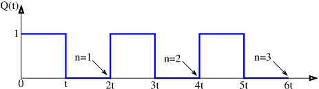
Figure S1: (Color online) The bang-bang protocol is visualized up to $n=3$. The arrows indicate the time instant when the overlap is calculated for an $n$th order protocol.

This leads to

$$|u^{(n)}_{q}(t)|^{2}=1+\left|\frac{v_{q}(t)}{2y_{q}(t)}\right|^{2}\left[\sum_{\sigma=\pm 1}\sigma\left(s_{q}(t)+\sigma y_{q}(t)\right)^{n}\right]^{2},$$ (S36)

where

$$y_{q}(t)=\sqrt{s^{2}_{q}(t)-1},\textmd{ }s_{q}(t)=\textmd{Re}\left(u_{q}(t)e^{-i\omega_{i}(q)t}\right),$$ (S37)

$$u_{q}(t)=\cos(\omega_{f}(q)t)-\frac{i}{2}\sin(\omega_{f}(q)t)\left(\frac{K_{i}}{K_{f}}+\frac{K_{f}}{K_{i}}\right)$$ (S38)

and $|v_{q}(t)|^{2}=|u_{q}(t)|^{2}-1$. By plugging Eq. (S36) to Eq. (9) in the main text, expanding the logarithm, then performing the momentum integral in the $t\gg\alpha/v_{f}$ limit, and finally resumming of the resulting series gives

$$\mathcal{L}_{n}(2nt)=\mathcal{L}_{SQ}^{n}(t)=\mathcal{L}_{ad}^{2n}.$$ (S39)

IV Additional properties of the Loschmidt echo

From Eqs. (10) and (13) in the main text, the LE is found to be symmetric with respect to the initial and final LL parameters in the steady state ($t\rightarrow\infty$) for adiabatic and sudden quenches as $(K_{i},K_{f})\longleftrightarrow(K_{f},K_{i})\longleftrightarrow(1/K_{i},1/K_{f})$. Since these hold true in the two extreme cases, it is plausible to assume that they remain valid for any smooth, monotonous protocol. Throughout the calculations, we have also assumed $L>vt$, otherwise revivals show up with a period $L/2v$.

Our adiabatic and SQ overlaps parallel closely to Anderson’s orthogonality catastrophe and the related x-ray edge singularity, respectively. However, while the overlap decays exponentially with the system size in our case, the impurity problem yields a power law suppression of the overlap with the system size or time.