Galactic cluster winds in presence of a dark energy

Abstract

We obtain a solution for the hydrodynamic outflow of the polytropic gas from the gravitating center, in presence of the uniform Dark Energy (DE). The antigravity of DE is enlightening the outflow and make the outflow possible at smaller initial temperature, at the same density. The main property of the wind in presence of DE is its unlimited acceleration after passing the critical point. In application of this solution to the winds from galaxy clusters we suggest that collision of the strongly accelerated wind with another galaxy cluster, or with another galactic cluster wind could lead to the formation of a highest energy cosmic rays.

1 Introduction

It was shown by Chernin (2001, 2008) that outer parts of galaxy clusters (GC) may be under strong influence of the dark energy (DE), discovered by observations of SN Ia at redshift $z\leq 1$ (Riess et al., 1998; Perlmutter et al., 1999), and in the spectrum of fluctuations of the cosmic microwave background radiation (CMB), see e.g. Spergel et al. (2003), Tegmark et al. (2004). Equilibrium solutions for polytropic configurations in presence of DE have been obtained in papers of Balaguera-Antolinez et al. (2006, 2007), and Merafina et al. (2012). The hot gas in the galactic clusters may flow outside due to high thermal pressure, and in the outer parts of the cluster the presence of a dark energy (DE) facilitates the outflow.

Here we obtain a solution of hydrodynamic equations for the winds from galactic clusters in presence of DE. We generalize the solution for the outflows from the gravitating body, obtained for solar and stellar winds by Stanyukovich (1955) and Parker (1963), to the presence of DE. It implies significant changes in the structure of solutions describing galactic winds.

2 Newtonian approximation in description galactic winds in presence of DE

A transition to the Newtonian limit, where DE is described by the antigravity force in vacuum was done by Chernin (2008). In the Newtonian approximation, in presence of DE, we have the following hydrodynamic Euler equation for the spherically symmetric outflow in the gravitational field of matter and DE

$$\rho v\frac{dv}{dr}+\frac{dP}{dr}=-\rho\left(\frac{Gm_{m}}{r^{2}}-\frac{\Lambda c^{2}r}{3}\right)=-\rho\left(\frac{Gm_{m}}{r^{2}}-\frac{8\pi G\rho_{\Lambda}r}{3}\right).$$ (1)

Here $\rho$ and $P$ are a matter density and pressure, respectively, $m_{m}$ is the mass of the matter inside the radius $r$. We use here DE in the form of the Einstein cosmological constant $\Lambda$. Newtonian gravitational potentials produced by matter $\Phi_{g}$, and $\Phi_{\Lambda}$ by DE, satisfy the Poisson equations

$$\Delta\Phi_{\Lambda}=-8\pi G\rho_{\Lambda},\quad\Delta\Phi_{g}=4\pi G\rho,\quad\rho_{\Lambda}=\frac{\Lambda c^{2}}{8\pi G}.$$ (2)

We consider, for simplicity, the outflow in the field of a constant mass (like in stellar wind) $m_{m}=M$. The Eq. (1) in this case is written as

$$\rho v\frac{dv}{dr}+\frac{dP}{dr}=-\rho\left(\frac{GM}{r^{2}}-\frac{\Lambda c^{2}r}{3}\right)=-\rho\left(\frac{GM}{r^{2}}-\frac{8\pi G\rho_{\Lambda}r}{3}\right).$$ (3)

The Eq. (1) should be solved together with the continuity equation in the form

$$4\pi\rho vr^{2}=\dot{M},$$ (4)

where $\dot{M}$ is the constant mass flux from the cluster. We consider polytropic equation of state, where pressure $P$, and sound speed $c_{s}$ are defined as

$$P=K\rho^{\gamma},\quad c_{s}^{2}=\gamma\frac{P}{\rho},\quad\rho=\left(\frac{c_{s}^{2}}{\gamma K}\right)^{\frac{1}{\gamma-1}},\quad P=\left(\frac{c_{s}^{2}}{\gamma}\right)^{\frac{\gamma}{\gamma-1}}K^{-\frac{1}{\gamma-1}}.$$ (5)

Introduce nondimensional variables as

$$\tilde{v}=\frac{v}{v_{*}}\quad\tilde{c}_{s}=\frac{c_{s}}{c_{*}},\quad\tilde{r}=\frac{r}{r_{*}},\quad r_{*}=\frac{GM}{c_{*}^{2}},\quad v_{*}=c_{*},$$ (6)

$$\tilde{\rho}=\frac{\rho}{\rho_{*}},\quad\tilde{P}=\frac{P}{P_{*}},\quad\rho_{*}=\left(\frac{c_{*}^{2}}{\gamma K}\right)^{\frac{1}{\gamma-1}},\quad P_{*}=\left(\frac{c_{*}^{2}}{\gamma}\right)^{\frac{\gamma}{\gamma-1}}K^{-\frac{1}{\gamma-1}}.$$

In non-dimensional variables the equation (3) is written as

$$\tilde{v}\frac{d\tilde{v}}{dr}+\frac{2}{\gamma-1}\tilde{c}_{s}\frac{d\tilde{c}_{s}}{d\tilde{r}}+\frac{1}{\tilde{r}^{2}}-\lambda\tilde{r}=0,\quad\lambda=\frac{\Lambda c^{2}r_{*}^{2}}{3c_{*}^{2}}.$$ (7)

The continuity equation (4) in non-dimensional form is written as

$$\tilde{\rho}\,\tilde{v}\,\tilde{r}^{2}=\dot{m},\quad\tilde{c}_{s}^{\frac{2}{\gamma-1}}\tilde{v}\tilde{r}^{2}=\dot{m},\quad\dot{m}=\frac{\dot{M}}{\dot{M}_{*}},\quad\dot{M}_{*}=4\pi\rho_{*}v_{*}r_{*}^{2}.$$ (8)

It follows from (5),(6),(8), that

$$\frac{d\tilde{\rho}}{\tilde{\rho}}=\frac{2}{\gamma-1}\frac{d\tilde{c}_{s}}{\tilde{c}_{s}},\quad\frac{d\tilde{\rho}}{\tilde{\rho}}+\frac{d\tilde{v}}{\tilde{v}}+2\frac{d\tilde{r}}{\tilde{r}}=0.$$ (9)

Using (9) we may write the equation of motion (7) in the form

$$\frac{d\tilde{v}}{d\tilde{r}}=\frac{\tilde{v}}{\tilde{r}}\,\frac{2\tilde{c}_{s}^{2}-\frac{1}{\tilde{r}}+\lambda\tilde{r}^{2}}{\tilde{v}^{2}-\tilde{c}_{s}^{2}}.$$ (10)

The only physically relevant solutions are those which pass smoothly the sonic point $v=c_{s}$, being a singular point of the Eq. (10), with

$$\tilde{v}=\tilde{c}_{s},\quad 2\tilde{c}_{s}^{2}-\frac{1}{\tilde{r}}+\lambda\tilde{r}^{2}=0$$ (11)

where $\tilde{r}=\tilde{r}_{c}$, $\tilde{v}=\tilde{v}_{c}$, $\tilde{c}_{s}=\tilde{c}_{sc}$. Choosing $c_{*}=c_{sc}$, we obtain in the critical point

$$\tilde{v}_{c}=\tilde{c}_{sc}=1,\quad 2-\frac{1}{\tilde{r}_{c}}+\lambda\tilde{r}_{c}^{2}=0.$$ (12)

With this choice of the scaling paraneters, we have from (8)

$$\dot{m}=\tilde{r}_{c}^{2}.$$ (13)

The relation (12) determining the dependence $\tilde{r}_{c}(\lambda)$ in the solution for the galactic wind and accretion, in presence of DE, is presented in Fig.1. The Eq.(7) for the polytropic flow has a Bernoulli integral as

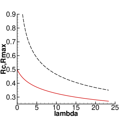
Figure 1: The functions $\tilde{r}_{c}(\lambda)$ (full curve), according to (12), and $\tilde{r}_{max}(\lambda)$ (dashed curve) according to (22). It is clear, that the critical radius of the flow $r_{c}$ is always inside the radius of the extremum of the total gravitational potential $r_{max}$.

$$\frac{\tilde{v}^{2}}{2}+\frac{\tilde{c}_{s}^{2}}{\gamma-1}-\frac{1}{\tilde{r}}-\frac{\lambda\tilde{r}^{2}}{2}=h,\quad\tilde{c}_{s}^{2}=\left(\frac{\dot{m}}{\tilde{v}\tilde{r}^{2}}\right)^{\gamma-1}=\left(\frac{\tilde{r}_{c}^{2}}{\tilde{v}\tilde{r}^{2}}\right)^{\gamma-1}.$$ (14)

The dimensional Bernoulli integral $H=hc_{sc}^{2}$. The Bernoulli integral is determined through the parameters of the critical point, with account of (12), as

$$h=\frac{\gamma+1}{2(\gamma-1)}-\frac{1}{\tilde{r}_{c}}-\frac{\lambda\tilde{r}_{c}^{2}}{2}=\frac{5-3\gamma}{2(\gamma-1)}-\frac{3}{2}\left(\frac{1}{\tilde{r}_{c}}-2\right).$$ (15)

The dependence $h(\lambda)$ for different polytropic powers $\gamma$ is given in Fig.2.

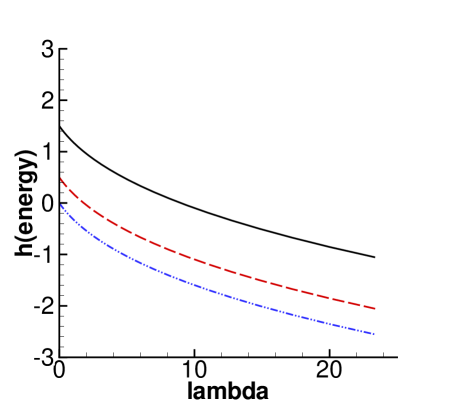
Figure 2: The function $h(\lambda)$ for $\gamma=\frac{4}{3}$ (full curve); $\gamma=\frac{3}{2}$ (dashed curve); $\gamma=\frac{5}{3}$ (dash-dot-dot curve), according to relations (12),(15).

The stationary solution for the wind is determined by two integrals: constant mass flux $\dot{M}$, and energy (Bernoulli) integral $H$. In absence of DE we obtain the known relations

$$\tilde{r}_{c}=\frac{1}{2},\quad h=\frac{5-3\gamma}{2(\gamma-1)}.$$ (16)

At small $\lambda$ we have from (12),(15)

$$\tilde{r}_{c}=0.5-\frac{\lambda}{16},\quad h=\frac{5-3\gamma}{2(\gamma-1)}-\frac{3}{8}\lambda$$ (17)

At large $\lambda\rightarrow\infty$ it follows from (12) $\tilde{r}_{c}\rightarrow\tilde{r}_{c\infty}=\lambda^{-1/3}$. Making expansion in (12) around $\tilde{r}_{c\infty}$ in the form

$$\frac{1}{\tilde{r}_{c}}=\lambda^{1/3}+\varepsilon,$$

we obtain from (12), (15)

$$\varepsilon=\frac{2}{3},\quad\tilde{r}_{c}=\frac{1}{\lambda^{1/3}+\frac{2}{3}},\quad h=\frac{5-3\gamma}{2(\gamma-1)}-\frac{3}{2}\lambda^{1/3}+2=\frac{\gamma+1}{2(\gamma-1)}-\frac{3}{2}\lambda^{1/3}\quad{\rm at}\quad\lambda\rightarrow\infty.$$ (18)

In the outflow from the physically relevant quasi-stationary object the antigravity from DE should be less the the gravitational force on the outer boundary, which we define at $r=r_{*}$. Therefore the value of $\Lambda$ is restricted by the relation (see e.g. Bisnovatyi-Kogan and Chernin, 2012)

$$2\rho_{\Lambda}=\frac{\Lambda c^{2}}{4\pi G}<\bar{\rho}=\frac{4\pi M}{3r_{*}^{3}}$$ (19)

In non-dimensional variables this restriction, with account of (6),(7) is written as

$$\lambda<\frac{16\pi^{2}}{9}=17.55=\lambda_{lim}.$$ (20)

It is reasonable to consider only the values of $\lambda$ smaller than $\lambda_{lim}$. It follows from (12), that $\tilde{r}_{c}$ is monotonically decreasing with increasing $\lambda$. For $\lambda\,=\,\lambda_{lim}=17.55$ we obtain $\tilde{r}_{c}=\tilde{r}_{c,lim}\approx 0.29$. The effective gravitational potential $\tilde{\Phi}$ is formed by the gravity of the central body, and antigravity of DE

$$\tilde{\Phi}=-\frac{1}{\tilde{r}}-\frac{\lambda\tilde{r}^{2}}{2}.$$ (21)

To overcome the gravity of the central body, the value of $h$ should exceed the maximum value of the gravitational potential, defined by the extremum of $\tilde{\Phi}$

$$h\geq\tilde{\Phi}_{max}(\tilde{r}_{max})=-\frac{3}{2}\lambda^{1/3},\quad\tilde{r}_{max}=\lambda^{-1/3}.$$ (22)

The function $\tilde{r}_{max}(\lambda)$ is represented in Fig.1, it is always $\tilde{r}_{max}>\tilde{r}_{c}$. So, in presence of DE the outflow of the gas from the cluster to the infinity is possible even at the negative values of $h$. In absence of DE the non-negative value of $h$, and the outflow are possible only at $\gamma\leq\frac{5}{3}$.

3 Solutions of the galactic wind equation in presence of DE

3.1 Analytical solutions

Analytical solutions exist only in absence of DE, $\Lambda=0$. In this case we have from (14)-(16)

$$\tilde{r}_{c}=\frac{1}{2},\quad h=\frac{\tilde{v}^{2}}{2}+\frac{\tilde{c}_{s}^{2}}{\gamma-1}-\frac{1}{\tilde{r}}=\frac{5-3\gamma}{2(\gamma-1)}.$$ (23)

For $\gamma=\frac{5}{3}$ the constant $h=0$ for the critical solution. At $h=0$ and $\gamma=\frac{5}{3}$ there is a whole family of solutions with arbitrary constant Mach number Ma=$\frac{v}{c_{s}}$ in all space. It is more convenient to write this solution in dimensional variables, with Bernoulli integral

$$H=\frac{v^{2}}{2}+\frac{3c_{s}^{2}}{2}-\frac{GM}{r}=0.$$ (24)

There is an exact solution in the form

$$v^{2}=\frac{2GM}{r}\frac{{\rm Ma}^{2}}{3+{\rm Ma^{2}}},\qquad c_{s}^{2}=\frac{2GM}{r}\frac{1}{3+{\rm Ma^{2}}}.$$ (25)

At Ma=1 this solution corresponds to the critical solutions for $\gamma=\frac{5}{3}$.

Another analytic solution takes place at $\gamma=1.5$, with the non-dimensional Bernoulli integral $h=0.5$. Using from (14), for $\gamma=1.5$, $r_{c}=0.5$,

$$\tilde{c}_{s}^{2}=\left(\frac{\tilde{r}_{c}^{2}}{\tilde{v}\tilde{r}^{2}}\right)^{\gamma-1}=\sqrt{\frac{1}{4\tilde{v}\tilde{r}^{2}}},$$

we obtain

$$h=\frac{\tilde{v}^{2}}{2}+\frac{1}{\tilde{r}\sqrt{\tilde{v}}}-\frac{1}{\tilde{r}}=\frac{1}{2}.$$

This nonlinear equation has two solutions

$${\bf 1.}\,\,\tilde{v}=1;\qquad{\bf 2.}\,\,\tilde{r}=\frac{2}{{\sqrt{\tilde{v}}}(1+\sqrt{{\tilde{v}}})(1+\tilde{v})}.$$ (26)

There, the first solution corresponds to the wind, and the second one corresponds to the accretion case, with negative velocity; $\tilde{v}$ in (26) represents the absolute value of this variable.

3.2 Numerical solution

To obtain a physically relevant critical solution of (10), with $\tilde{c}_{s}^{2}$ from (14), we obtain expansion in the critical point with $\tilde{v}^{2}=\tilde{c}_{s}^{2}=1$, in the form

$$\tilde{v}=1+\alpha(\tilde{r}-\tilde{r}_{c}),\quad\alpha_{1}=-\frac{2}{\tilde{r}_{c}}\frac{\gamma-1}{\gamma+1}+\frac{1}{\tilde{r}_{c}}\frac{2}{\gamma+1}\sqrt{2+\frac{1}{4\tilde{r}_{c}}+\frac{\lambda\tilde{r}_{c}^{2}}{2}-\gamma\left(2-\frac{1}{4\tilde{r}_{c}}-\frac{\lambda\tilde{r}_{c}^{2}}{2}\right)},$$ (27)

$$\qquad\qquad\alpha_{2}=-\frac{2}{\tilde{r}_{c}}\frac{\gamma-1}{\gamma+1}-\frac{1}{\tilde{r}_{c}}\frac{2}{\gamma+1}\sqrt{2+\frac{1}{4\tilde{r}_{c}}+\frac{\lambda\tilde{r}_{c}^{2}}{2}-\gamma\left(2-\frac{1}{4\tilde{r}_{c}}-\frac{\lambda\tilde{r}_{c}^{2}}{2}\right)}.$$

Here $\alpha_{1}$ corresponds to the wind solution, and $\alpha_{2}$ is related to the case of accretion where $\tilde{v}$ define the absolute value. At $\lambda=0$ we have a well known expansion with

$$\alpha_{1}=\frac{4}{\gamma+1}\left[\sqrt{\frac{5-3\gamma}{2}}-(\gamma-1)\right],$$

$$\alpha_{2}=-\frac{4}{\gamma+1}\left[\sqrt{\frac{5-3\gamma}{2}}+(\gamma-1)\right].$$

It follows from the expansion (27), that physically relevant solutions exist only with positive value under the square root. It give the restriction for the value of $\gamma$ as a function of $\lambda$ in the form

$$\gamma\leq\gamma_{max}=\frac{2+\frac{1}{4\tilde{r}_{c}}+\frac{\lambda\tilde{r}_{c}^{2}}{2}}{2-\frac{1}{4\tilde{r}_{c}}-\frac{\lambda\tilde{r}_{c}^{2}}{2}}.$$

At $\lambda=32$, $\tilde{r}_{c}=0.25$ the limiting value $\gamma_{max}$ goes to $\infty$, so that at $\lambda\geq 32$ the wind solutions exist formally for all polytropic powers $\gamma$. The dependence $\gamma_{max}(\lambda)$ is given in Fig.3.

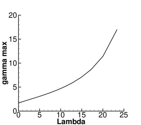
Figure 3: The functions $\gamma_{max}(\lambda)$. The smooth solution for the outflow from the gravitating center, in presence of DE, is possible only at $\gamma\leq\gamma_{max}$.

The critical solutions of the equation (10), with account of (14), are presented in Figs.4-6 for different values of $\gamma$ and $\lambda$. Both wind and accretion solutions are presented.

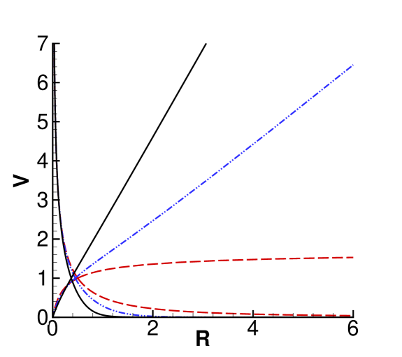
Figure 4: The integral curves of the equations (10), (14), for $\gamma=4/3$ and $\lambda=0$, $r_{c}$=0.5 (dashed curves); $\lambda=1.10$, $r_{c}=0.45$ (dash-dot-dot curves); and $\lambda=5.13$, $r_{c}=0.37$ (full curves). Wind solutions correspond to curves with increasing velocity at large radius. The curves with decreasing velocities correspond to the accretion solution with negative $v$, so that its absolute value is presented.

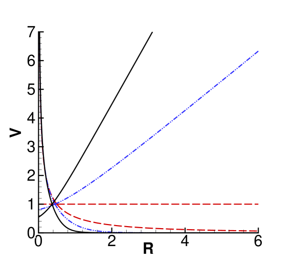
Figure 5: The integral curves of the equations (10), (14), for $\gamma=3/2$ and $\lambda=0$, $r_{c}$=0.5 (dashed curves); $\lambda=1.10$, $r_{c}=0.45$ (dash-dot-dot curves); and $\lambda=5.13$, $r_{c}=0.37$ (full curves). Wind solutions correspond to curves with increasing (or constant) velocity at large radius. The curves with decreasing velocities correspond to the accretion solution with negative $v$, so that its absolute value is presented.

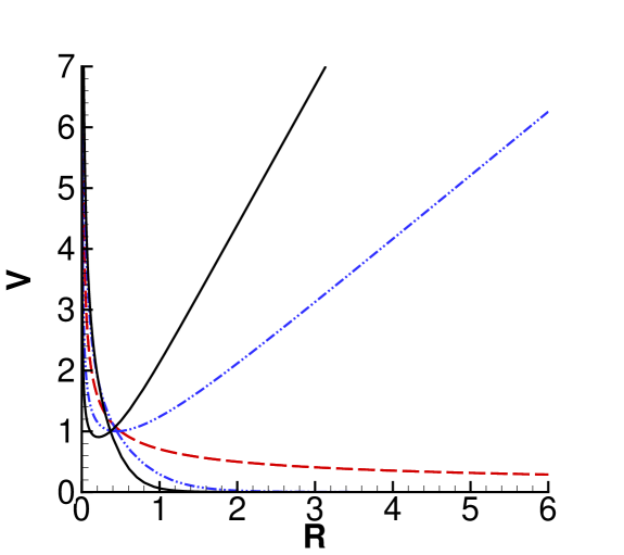
Figure 6: The integral curves of the equations (10), (14), for $\gamma=5/3$ and $\lambda=0$, $r_{c}$=0.5 (dashed curve); $\lambda=1.10$, $r_{c}=0.45$ (dash-dot-dot curves); and $\lambda=5.13$, $r_{c}=0.37$ (full curves). For nonzero $\lambda$ wind solutions correspond to curves with increasing velocity at large radius. The curves with decreasing velocities correspond to the accretion solution with negative $v$, so that its absolute values are presented. At $\lambda=0$ both wind and accretion solutions are presented by the same curve, which corresponds to the wind for positive $v$, and to the accretion for negative $v$.

4 Discussion

It is clear that the presence of DE tends to help the outflow of the hot gas from the gravitating object, as well as to the escape of rapidly moving galaxies (Chernin et al, 2013). Here we have obtained the solution for outflow in presence of DE, which generalize the well-known solution for the polytropic solar (stellar) wind. Presently the DE density exceed the density of the dark matter, and, even more, the density of the barionic matter. The clusters which outer radius is approaching the zero gravity radius, may not only loose galaxies, which join the process of Hubble expansion, but also may loose the hot gas from the outer parts of the cluster. Let us consider outer parts of the Coma cluster at radius $R_{C}=15$ Mpc, with the mass inside $M_{C}=5\cdot 10^{15}\,M_{\odot}$, from Chernin et al. (2013). For the present value of $\rho_{\Lambda}=0.71\cdot 10^{-29}$ g/cm³, supposing that $R_{C}=r_{*}$ is the critical radius of the wind, we obtain from (2),(7), the nondimensional constant $\lambda$ as

$$\lambda=\frac{\Lambda c^{2}r_{*}^{2}}{3c_{*}^{2}}=\frac{8\pi}{3}\frac{\rho_{\Lambda}r_{*}^{3}}{M}\approx 0.59,\quad c_{*}=\sqrt{\frac{G\,M_{C}}{R_{C}}}\approx 1200\,\,{\rm km/c}.$$ (28)

It corresponds to the temperature about $T\approx 6\cdot 10^{7}$ K, $kT\approx 5$ keV. Observations of the hot gas distribution in the Coma cluster (Watanabe et al., 1999) on ASCA satellite have shown a presence of hot region with $kT=11-14$ keV, and more extended cool region with $kT=5\pm 1$ keV, what is in good accordance with our choice of parameters.

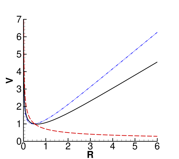
Figure 7: The integral curves of the equations (10), (14) for the wind solution, at $\gamma=5/3$ and $\lambda=0$, $r_{c}$=0.5 (dashed curve); $\lambda=1.10$, $r_{c}=0.45$ (dash-dot-dot curves); and $\lambda=0.58$, $r_{c}=0.47$ (full curves).

Wind solutions for $\lambda$=0; 0.58; 1.1 are presented in Fig.7. The solution with $\lambda$=0.58 is the closest to the description of the outflow from Coma cluster. The density of the gas in the vicinity of $r=r_{c}$ is very small, so the flow may be considered as adiabatic (polytropic) with the power $\gamma$=5/3. Without DE such gas flow is inefficient, its velocity is decreasing $\sim 1/\sqrt{r}$, see Eq. (25). In presence of DE the wind velocity is increasing  2 times at the distance of $\sim 5r_{c}\sim 75$ Mpc from Coma.

After quitting the cluster the gas is moving with acceleration, acting as a snowplough for the intergalactic gas. The shell of matter, forming in such a way, may reach a high velocity, exceeding considerably the speed of galaxies in cluster. If the shell meets another cluster, or another shell moving towards, the collision of such flows may induce a particle acceleration. Due to high speed, large sizes, and low density such collisions may create cosmic rays of the highest possible energy (EHECR). We may expect the largest effect when two clusters move to each other. The influence of DE is decreasing with with a red shift, therefore the acceleration of EHECR in this model should take place in the periphery, or between, the closest rich galaxy clusters.

References

- (1) Balaguera-Antolínez, A., Mota, D.F., Nowakowski, M. 2006, Class. Quant. Grav., 23, 4497
- (2) Balaguera-Antolínez, A., Mota, D.F., Nowakowski, M. 2007, MNRAS, 382, 621
- (3) Bisnovatyi-Kogan, G. S. 2010, Stellar Physics. II. Stellar Structure and Stability. Heidelberg: Springer (2d Edition)
- (4) Bisnovatyi-Kogan, G.S., Chernin, A.D. 2012, ApSS, 338, 337
- (5) Chernin A.D. 2001, Physics-Uspekhi 44, 1099
- (6) Chernin A.D. 2008, Physics-Uspekhi, 51, 267
- (7) Chernin A.D., Bisnovatyi-Kogan G.S., Teerikorpi P., Valtonen M.J., Byrd G.G., Merafina M. 2013, Astron. Ap.(accepted). Astro-ph 1303.3800.
- (8) Merafina, M, Bisnovatyi-Kogan, G.S. & Tarasov, S.O. 2012, Astron. Ap. 541, 84
- (9) Parker I. E. N. , 1963, Interplanetary dynamical processes. New York, Interscience Publishers
- (10) Perlmutter S. et al. 1999, Astrophys. J. 517, 565
- (11) Riess A. G. et al. 1998, Astron. J. 116, 1009
- (12) Spergel D N et al. 2003, Astrophys. J. Suppl. 148, 175
- (13) Stanyukovich K.P., 1955, Unsteady Motions of Continua [in Russian], Gostekhizdat
- (14) Tegmark M. et al. 2004, Phys. Rev. D69, 103501
- (15) Watanabe M. et al. 1999, Astrophys. J. 527, 80