Crossover from adiabatic to antiadiabatic phonon-assisted tunneling in single-molecule transistors

Abstract

The crossover between two customary limits of phonon-assisted tunneling, the adiabatic and antiadiabatic regimes, is studied systematically in the framework of a minimal model for molecular devices: a resonant level coupled by displacement to a localized vibrational mode. Conventionally associated with the limits where the phonon frequency is either sufficiently small or sufficiently large as compared to the bare electronic hopping rate, we show that the crossover between the two regimes is governed for strong electron-phonon interactions primarily by the polaronic shift rather than the phonon frequency. In particular, the perturbative adiabatic limit is approached only as the bare hopping rate $\Gamma$ exceeds the polaronic shift, leaving an extended window of couplings where $\Gamma$ well exceeds the phonon frequency and yet the physics is basically that of the antiadiabatic regime. We term this intermediate regime the extended antiadiabatic regime. The effective low-energy Hamiltonian in the traditional and the extended antiadiabatic regime is shown to be the (purely fermionic) interacting resonant-level model, with parameters that we extract from numerical renormalization-group calculations. The extended antiadiabatic regime is followed in turn by a true crossover region where the polaron gets progressively undressed. In this latter region, the phonon configuration strongly deviates from a simple superposition of just one or two coherent states. The renormalized tunneling rate, which serves as the low-energy scale in the problem and thus sets the width of the tunneling resonance, is found to follow an approximate scaling form on going from the adiabatic to the antiadiabatic regime. Charging properties are governed by two distinct mechanisms at the extended antiadiabatic and into the crossover region, giving rise to characteristic shoulders in the low-temperature conductance as a function of gate voltage. These shoulders serve as a distinct experimental fingerprint of phonon-assisted tunneling when the electron-phonon coupling is strong.

I Introduction

The promise of molecular electronics has focused enormous interest on molecular devices. Reviews Typically, such devices consist of an individual molecule trapped between two leads, in-between which a voltage bias is applied. By measuring the current flowing across the molecular bridge one can investigate the molecule’s internal degrees of freedom and their coupling to the leads, which can lead in turn to complex many-body physics. While lacking the exquisite design and control capabilities of semiconductor quantum dots, molecular devices can be produced in large quantities, thus allowing for many samples to be scanned in a relatively short period of time. At the same time, it is not always clear if a molecule has been successfully trapped between the leads, or whether it might have been damaged or distorted in the course of preparation.

From a basic-science perspective, single-molecule transistors (SMT) offer two major advantages over their semiconductor counterparts. First, the relevant energy scales are notably larger in SMTs, rendering these scales more accessible to experiments. Second, the electronic degrees of freedom are generally coupled to nuclear vibrational modes, providing an extraordinary opportunity to study the electron-phonon coupling at the nano-scale. The same picture applies to suspended carbon nanotubes, where the motion of electrons is coupled to vibrations of the tube (vibrons). Indeed, phonon-assisted tunneling can lead to a plethora of interesting phenomena, including the appearance of inelastic steps and peaks in the differential conductance, ZMB02 ; QNH04 ; Natelson-04 ; Sapmaz-etal-06 ; Tal-etal-08 the Frank-Condon blockade, Sapmaz-etal-06 ; Leturcq-etal-09 and the interplay with the Kondo effect. YN04 ; Parks-et-al-07 ; Natelson-review While most of the experiments cited above are in general accord with theoretical expectations, some issues, such as the sign of the inelastic steps at integer multiples of the phonon frequency, remain under debate. EG08 ; EWIA09 Other theoretical predictions awaiting experimental verification include unorthodox variants of the Kondo effect, Cornaglia-et-al ; Two-channel-SMT signatures of pair tunneling, KRvO06 and interesting nonequilibrium effects on the phonon distribution function, Koch-et-al-06 to name but a few.

While much of the theoretical activity on molecular devices is presently centered on finite-bias transport, in this paper we focus on thermal equilibrium and address a specific question pertaining to the nature of the crossover between two customary limits of phonon-assisted tunneling, the so-called adiabatic and antiadiabatic regimes. These two terms are broadly used in the context of electron-phonon coupling to indicate the limits where the bare electronic motion is either sufficiently fast (adiabatic limit) or sufficiently slow (antiadiabatic limit) as compared to the phonon vibrations. In the more specific context of resonant phonon-assisted tunneling, the relevant measure of electronic motion is given by the tunneling rate. Hence, the two limits correspond to whether the bare electronic tunneling rate $\Gamma$ is either sufficiently small or sufficiently large as compared to the phonon frequency $\omega_{0}$.

When $\Gamma\ll\omega_{0}$ (we work with units in which $\hbar=1$), the phonon can efficiently respond to hopping events by forming a polaron, suppressing thereby the electronic tunneling rate. This suppression, which can be quite dramatic, is manifest, e.g., in a narrowing of the tunneling resonance. In the opposite limit, $\omega_{0}\ll\Gamma$, the phonon is too slow to respond to the frequent tunneling events, having little effect on their rate. Each of these extreme limits is rather well controlled theoretically, either in the framework of the Lang-Firsov transformation LF62 or using ordinary perturbation theory in the electron-phonon coupling. Far less understood is the crossover region between the two limits, which lacks a small parameter.

This general picture neglects, however, another important energy scale: the harmonic potential energy associated with the relative displacement of the phonon between different molecular electronic configurations. In the case of a single spinless level with the dimensionless displacement coupling $\lambda$ [see Eq. (1) for an explicit definition of $\lambda$], the so-called polaronic shift is given by $E_{\rm p}=\lambda^{2}\omega_{0}$. Thus, depending on the magnitude of $\lambda$, the polaronic shift $E_{\rm p}$ may exceed $\Gamma$ and/or $\omega_{0}$. Quantum mechanically it is natural to associate $E_{\rm p}$ with a new time scale $\tau_{\rm p}=1/E_{\rm p}$, which may either be shorter or longer than the electronic dwell time $\tau_{\rm dwell}=1/\Gamma$ and the period of oscillations $\tau_{\rm osc}=2\pi/\omega_{0}$. Whether $\tau_{\rm p}$ has the status of a true physical time scale is not immediately clear. It can not have real significance for $\lambda\ll 1$, when the phonon displacement is small as compared to its zero-point motion. Neither does $\tau_{\rm p}$ play any role for a classical oscillator, whose period is independent of the amplitude of oscillations. At the same time, $E_{\rm p}$ does show up as an additional energy scale for phonon-assisted tunneling, Selman although its significance, let alone its role in defining the physical boundaries of the adiabatic and antiadiabatic regimes, have never been quite resolved.

From this brief discussion it is clear that the most interesting and yet most challenging regime is that of strong electron-phonon coupling, $1\ll\lambda$, where $\tau_{\rm p}$, whatever its physical interpretation might be, can potentially assume a dominant role. The interest in strong electron-phonon coupling is further amplified by recent reports of large values of $\lambda$ (including some in excess of 5) in suspended carbon nanotubes. Leturcq-etal-09 In the antiadiabatic limit, the tunneling electrons experience strong polaronic dressing for $1\ll\lambda$, reflected in an exponential suppression of the renormalized tunneling rate from $\Gamma$ to $\Gamma_{\rm eff}=\Gamma e^{-\lambda^{2}}\ll\Gamma$. This dramatic effect raises several basic questions:

1. When tuning the bare tunneling rate from weak ($\Gamma\ll\omega_{0}$) to strong ($\omega_{0}\ll\Gamma$) coupling, which physical parameters set the scale for first leaving the polaronic physics of the antiadiabatic regime and then entering the perturbative physics of the adiabatic regime? Are these two transitions governed by a single scale or are there perhaps two distinct scales?

2. How does the ratio $\Gamma_{\rm eff}/\Gamma$ evolve from its exponentially small value $e^{-\lambda^{2}}$ in the antiadiabatic regime back to approximately one in the adiabatic limit? In other terms, how does the polaron get undressed?

3. Are there any distinct experimental signatures of the crossover regime that can be detected?

I.1 Preliminaries

In this paper, we answer these questions in detail in the framework of the resonant-level model with an additional displacement coupling to a localized vibrational mode [see Eq. (1)]. Besides being one of the most widely used models for single-molecule devices, our motivation for adopting this specific Hamiltonian is two-fold. The first is physical clarity, as this Hamiltonian constitutes the minimal model where the crossover from the antiadiabatic to the adiabatic regime of phonon-assisted tunneling can be studied without being masked by competing many-body effects (e.g., the Kondo effect in case of a spinful level). The second point is technical in nature, and pertains to our method of choice for accurate nonperturbative calculations. In this work we employ Wilson’s numerical renormalization-group (NRG) approach, Wilson75 ; BCP08 which is a highly precise tool for calculating equilibrium properties of quantum impurity systems. In the NRG, the computational effort grows exponentially with the number of conduction-electron species, hence the restriction to a single spinless band allows us to accurately address large values of $\lambda$ that otherwise would be inaccessible using more elaborate models.

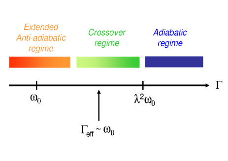
Figure 1: (Color online) Schematic description of the crossover from the antiadiabatic to the adiabatic regime of resonant phonon-assisted tunneling, for strong electron-phonon interactions $1\ll\lambda$. Upon increasing $\Gamma$, an extended antiadiabatic regime persists until the renormalized tunneling rate $\Gamma_{\rm eff}$ approaches the phonon frequency $\omega_{0}$. The condition $\Gamma_{\rm eff}=\omega_{0}$ is typically met for $\Gamma\sim 0.55E_{\rm p}$ with $E_{\rm p}=\lambda^{2}\omega_{0}$, extending the physics of the antiadiabatic regime far beyond the traditional condition $\Gamma<\omega_{0}$. In terms of the bare model parameters, the extended antiadiabatic regime persists up to $\Gamma\sim 0.4E_{\rm p}$. The perturbative physics of the adiabatic regime is approached only as $\Gamma$ exceeds $E_{\rm p}$, leaving an intermediate crossover region for $0.4E_{\rm p}\lesssim\Gamma\lesssim E_{\rm p}$ where the polaron gets progressively undressed. The phonon configuration strongly deviates in the crossover region from a simple superposition of just one or two coherent states.

We note in passing that the NRG has been applied to moderately large values of $\lambda$ in the framework of the spinful Anderson-Holstein model, HM02 however, these studies used rather large values of the phonon frequency. The combination of large values of $\lambda$ and small phonon frequencies (as is appropriate for molecular and nanotube devices) is presently a challenge to treat accurately using the NRG if spin is to be included.

Focusing on $1\ll\lambda$, Fig. 1 displays our resulting scenario for the crossover from the antiadiabatic to the adiabatic regime. In contrast to the naive picture, the crossover is governed primarily by the polaronic shift $E_{\rm p}$ rather than the phonon frequency $\omega_{0}$. In particular, the perturbative adiabatic limit is approached only as $\Gamma$ exceeds $E_{\rm p}$, leaving a rather broad window of couplings where $\Gamma$ well exceeds $\omega_{0}$ and yet the physics is basically that of the antiadiabatic regime. We term this intermediate regime the extended antiadiabatic regime.

The physical origin of the extended antiadiabatic regime is in the enormous separation of scales between $\Gamma$ and $\Gamma_{\rm eff}$ when $\Gamma\ll E_{\rm p}$. Although smaller than the bare tunneling rate, the phonon frequency $\omega_{0}$ remains notably larger than the renormalized one, hence the phonon can still efficiently respond to the individual tunneling events. The distinction between the extended and the traditional antiadiabatic regimes is therefore quantitative rather than qualitative, both being described by the same fermionic interacting resonant-level model at energies below $\omega_{0}$. For this reason, we have lumped the two regimes into one in Fig. 1. In terms of the bare model parameters, the extended antiadiabatic regime persists up to $\Gamma\sim 0.4E_{\rm p}$, breaking down as $\Gamma_{\rm eff}$ approaches $\omega_{0}$ in magnitude. The extended antiadiabatic regime and the adiabatic one are separated in turn by a true crossover region for $0.4E_{\rm p}\lesssim\Gamma\lesssim E_{\rm p}$, where the polaron gets progressively undressed. The phonon configuration strongly deviates in this region from a simple superposition of just one or two coherent states, as we show by explicit calculations.

I.2 Plan of the paper

After introducing the Hamiltonian and its symmetries in Sec. II, we proceed in Sec. III to a preliminary discussion of certain limits where analytic insight can be gained. These include the traditional adiabatic and antiadiabatic limits, the extended antiadiabatic regime proposed in this paper, and the limit of large detuning. Section IV presents in turn a systematic study of all coupling regimes using Wilson’s NRG. To this end, we begin with a brief introduction of the method in Sec. IV.1, followed by an extensive investigation of the key quantities of interest: the renormalized tunneling rate $\Gamma_{\rm eff}$, the mapping onto an effective low-energy interacting resonant-level model in the antiadiabatic and the extended antiadiabatic regimes, charging of the level, and the phonon distribution function defined in Eq. (35). We conclude in Sec. VI with a summary of our results. Some technical details are deferred to two appendices.

II The model and its symmetries

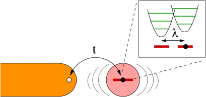
Figure 2: (Color online) The physical system under consideration. A localized level with energy $\epsilon_{d}$ is tunnel coupled with amplitude $t$ to a band of spinless electrons, and is simultaneously coupled by a dimensionless displacement coupling $\lambda$ to a single vibrational mode of frequency $\omega_{0}$. Depending on the valence of the level, the vibrational mode experiences a shifted harmonic potential with a relative displacement of $\Delta b=\lambda$.

The system under consideration is shown schematically in Fig. 2. It consists of a single localized electronic level $d^{\dagger}$ with energy $\epsilon_{d}$, tunnel coupled to a continuous band of noninteracting spinless electrons which we denote by $c^{\dagger}_{k}$. The level is simultaneously coupled by displacement to a localized vibrational mode (phonon), as modeled by the Hamiltonian

$${\cal H} = \sum_{k}\epsilon_{k}c^{\dagger}_{k}c_{k}+\frac{t}{\sqrt{N}}\sum_{k}\left\{d^{\dagger}c_{k}+{\rm H.c.}\right\}+\epsilon_{d}d^{\dagger}d$$ (1)

$$+\omega_{0}b^{\dagger}b+\lambda\omega_{0}\left(d^{\dagger}d-N_{0}\right)\left(b^{\dagger}+b\right).$$

Here, $b^{\dagger}$ creates a local Einstein phonon that oscillates with frequency $\omega_{0}$, $t$ is the tunneling matrix element between the level and the Wannier state closest to the molecule, and $N$ is the number of lattice sites. The dimensionless coupling $\lambda$ measures the relative displacement of the vibrational mode between the configurations where the level is empty and occupied. It serves as a faithful measure for the strength of the electron-phonon coupling, with $\lambda\ll 1$ ($1\ll\lambda$) corresponding to weak (strong) interactions. The parameter $N_{0}$ can be thought of as fixing the reference charge of the level. It can be formally eliminated by shifting the bosonic mode according to $\hat{B}=b-\lambda N_{0}$, which has the effect of renormalizing the level energy from its bare value $\epsilon_{d}$ to $\tilde{\epsilon}_{d}$ with

$$\tilde{\epsilon}_{d}=\epsilon_{d}+2N_{0}\lambda^{2}\omega_{0}.$$ (2)

The conversion from $b$ to $B$ also generates the constant term $-N_{0}\lambda^{2}\omega_{0}$, which uniformly shifts the spectrum of the Hamiltonian. Although the inclusion of $N_{0}$ adds no richness to the thermodynamics of the model, it provides a useful tuning parameter for exploring the low-energy state of the system, as will be demonstrated later on.

In the following we shall consider a particle-hole symmetric band, namely, it is assumed that the wave numbers can be grouped into distinct pairs $k$ and $k^{\prime}$, such that $\epsilon_{k^{\prime}}=-\epsilon_{k}$ for each pair of momenta. It is easy to verify that the combined transformation

$$d^{\dagger}\to d,\;\;\;c^{\dagger}_{k}\to-c_{k^{\prime}},\;\;\;{\rm and}\;\;\;b\to-b-\lambda(1-2N_{0})$$ (3)

leaves the Hamiltonian of Eq. (1) unchanged under these terms, apart from the substitution comment-on-shift-I

$$\epsilon_{d}\to\tilde{\epsilon}_{d}=2\lambda^{2}\omega_{0}(1-2N_{0})-\epsilon_{d}.$$ (4)

It therefore suffices to study the domain $\epsilon_{d}\geq\epsilon_{d}^{\ast}$ with

$$\epsilon_{d}^{\ast}=\lambda^{2}\omega_{0}(1-2N_{0}),$$ (5)

while the complementary domain $\epsilon_{d}<\epsilon_{d}^{\ast}$ is accessible via the particle-hole transformation of Eq. (3). In particular, occupancy of the level $n_{d}(\epsilon_{d})=\langle d^{\dagger}d\rangle$ obeys the symmetry relation

$$n_{d}(\epsilon_{d}^{\ast}-\Delta\epsilon_{d})=1-n_{d}(\epsilon_{d}^{\ast}+\Delta\epsilon_{d}),$$ (6)

independent of all other model parameters, the temperature included.

Other than the conduction-electron bandwidth $D$, the Hamiltonian of Eq. (1) features four basic energy scales. These include the bare vibrational frequency $\omega_{0}$, the polaronic shift $E_{\rm p}=\lambda^{2}\omega_{0}$, the detuning energy $\Delta\epsilon_{d}=\epsilon_{d}-\epsilon_{d}^{\ast}$, and the hybridization width $\Gamma=\pi\rho_{0}t^{2}$. Here $\rho_{0}$ is the conduction-electron density of states at the Fermi level. comment-on-DOS Of particular interest is the point $\Delta\epsilon_{d}=0$, when the (renormalized) level lies at resonance with the Fermi energy. The relevant low-energy scale in the problem is conveniently defined BSZ08 in this case from the zero-temperature charge susceptibility evaluated at $\epsilon_{d}^{\ast}$:

$$\Gamma_{\rm eff}=\frac{1}{\pi\chi_{\rm c}},$$ (7)

with

$$\chi_{c}=\left.-\frac{dn_{d}}{d\epsilon_{d}}\right|_{\epsilon_{d}=\epsilon_{d}^{\ast}}.$$ (8)

For $\lambda=0$, the low-energy scale $\Gamma_{\rm eff}$ so defined coincides with the bare hybridization width $\Gamma$. Various thermodynamic properties associated with the level, e.g., its occupancy and its contribution to the electronic specific heat, reduce in the wide-band limit to exclusive functions of $\epsilon_{d}/\Gamma$ and $T/\Gamma$, where $T$ is the temperature. A nonzero $\lambda$ modifies this picture both qualitatively and quantitatively. For example, occupancy of the level at $T=0$ is no longer given for large $\lambda$ by an exclusive function of $\Delta\epsilon_{d}/\Gamma_{\rm eff}$, but rather depends, as we shall show, on vastly different energy scales. Our goal is to conduct a systematic study of all coupling regimes for nonzero $\lambda$, focusing primarily on large $\lambda$. To this end, we shall combine analytical considerations with Wilson’s renormalization-group (NRG) method. Wilson75 ; BCP08

III Limiting cases

We begin with a preliminary discussion of certain limits where analytic insight can be gained. These include the traditional adiabatic and antiadiabatic limits, the proposed extended antiadiabatic regime where $\omega_{0}<\Gamma$ but $\Gamma_{\rm eff}\ll\omega_{0}$, and the limit of large detuning, $\Gamma\ll|\epsilon_{d}|$.

III.1 Adiabatic limit

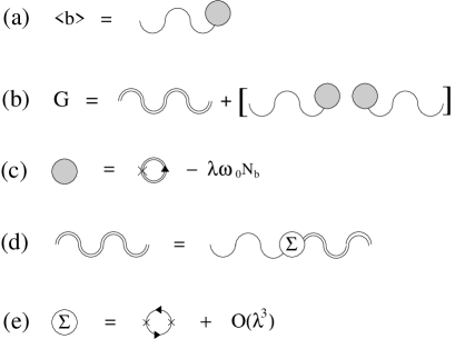
Figure 3: Diagrammatic representation of (a) the phononic expectation value $\langle b\rangle$ and (b) the phononic Green’s function $G(i\nu_{n})$. Here, single (double) wiggly lines represent the bare (dressed) connected phonon propagator $\tilde{G}(i\nu_{n})$, whereas single (double) lines with an arrow denote the bare (dressed) $d$-electron propagator (bare/dressed with respect to $\lambda$; both electronic propagators are dressed with respect to $t$ alone). The connected phonon propagator $\tilde{G}(i\nu_{n})$ obeys a standard Dyson equation (d), with a matrix self-energy $\hat{\Sigma}$ whose second-order expansion in $\lambda$ is specified in panel (e). Interaction vertices are marked by a cross.

Commencing with the limit of small $\lambda$, we apply ordinary perturbation theory in the electron-phonon coupling $\lambda$, postponing for the moment the question of its range of validity. The basic quantity of interest is the Matsubara phonon propagator

$$G(i\nu_{n})=\left[\begin{array}[]{cc}G_{bb^{\dagger}}(i\nu_{n})&G_{bb}(i\nu_{n})\\ \\ G_{b^{\dagger}b^{\dagger}}(i\nu_{n})&G_{b^{\dagger}b}(i\nu_{n})\end{array}\right],$$ (9)

where $\nu_{n}=2\pi n/\beta$ are the bosonic Matsubara frequencies, $\beta=1/k_{\rm B}T$ is the reciprocal temperature, and

$$G_{AB}(i\nu_{n})=-\int_{0}^{\beta}\langle T_{\tau}\hat{A}(\tau)\hat{B}(0)\rangle e^{i\nu_{n}\tau}d\tau.$$ (10)

Using the diagrams specified in Fig. 3, one obtains the formally exact relations

$$\langle b\rangle=-\lambda\left[\langle d^{\dagger}d\rangle-N_{0}\right]$$ (11)

and

$$G_{\alpha\gamma}(i\nu_{n})=\tilde{G}_{\alpha\gamma}(i\nu_{n})-\delta_{n,0}\beta\lambda^{2}\left[\langle d^{\dagger}d\rangle-N_{0}\right]^{2},$$ (12)

where $\tilde{G}(i\nu_{n})$ is the connected phonon propagator, defined as the sum of all connected phonon diagrams. The connected propagator has the conventional representation $\tilde{G}^{-1}=[\tilde{G}^{(0)}]^{-1}-\hat{\Sigma}$, where

$$\left[\tilde{G}^{(0)}(i\nu_{n})\right]^{-1}=\left(\begin{array}[]{cc}i\nu_{n}-\omega_{0}&0\\ \\ 0&-i\nu_{n}-\omega_{0}\end{array}\right)$$ (13)

is the unperturbed phonon Green’s function and $\hat{\Sigma}$ is the self-energy matrix. Since the electron-phonon interaction in Eq. (1) involves only the combination $b+b^{\dagger}$, the self-energy matrix takes the general form

$$\hat{\Sigma}(i\nu_{n})=\sigma(i\nu_{n})\left(\begin{array}[]{cc}1&1\\ 1&1\end{array}\right),$$ (14)

which depends on a single scalar function $\sigma(i\nu_{n})$. Settling with second order in $\lambda$ and analytically continuing to real frequencies, $\sigma(\omega+i\eta)$ is given for $T\to 0$ in the wide-band limit by

$$\sigma(\omega+i\eta)=\frac{\lambda^{2}\omega_{0}^{2}}{2i\pi}\left[I_{-}(\omega)-I_{-}^{\ast}(-\omega)-I_{+}(\omega)+I_{+}^{\ast}(-\omega)\right],$$ (15)

where

$$I_{+}(\omega)=\frac{1}{\omega}\left[\ln(-\epsilon_{d}+i\Gamma)-\ln(\omega-\epsilon_{d}+i\Gamma)\right]$$ (16)

and

$$I_{-}(\omega)=\frac{1}{\omega+2i\Gamma}\left[i\pi+\ln(\epsilon_{d}+i\Gamma)-\ln(\omega-\epsilon_{d}+i\Gamma)\right].$$ (17)

Focusing on the resonance condition $\epsilon_{d}=0$ and expanding in powers of the frequency, comment-on-resonance $\sigma(\omega+i\eta)$ reads as

$$\sigma(\omega+i\eta)=-\frac{\lambda^{2}\omega_{0}^{2}}{\pi\Gamma}-i\omega\frac{\lambda^{2}\omega_{0}^{2}}{\pi\Gamma^{2}}+{\cal O}(\omega^{2}),$$ (18)

resulting in

$$\tilde{G}^{-1}(\omega+i\eta)=\left[\begin{array}[]{cc}(1\!+\!i\gamma)\omega\!-\!\omega_{0}\!+\!A&i\gamma\omega\!+\!A\\ \\ i\gamma\omega\!+\!A&(i\gamma\!-\!1)\omega\!-\!\omega_{0}\!+\!A\end{array}\right]$$ (19)

with $\gamma=\lambda^{2}\omega_{0}^{2}/(\pi\Gamma^{2})$ and $A=\lambda^{2}\omega_{0}^{2}/(\pi\Gamma)$. The poles of $\tilde{G}(z)$ can now be identified with the zeros of ${\rm det}\{\tilde{G}^{-1}(z)\}$, which yields

$$z_{\pm}=-i\frac{\omega_{0}}{\pi}\left(\frac{\lambda\omega_{0}}{\Gamma}\right)^{2}\pm\omega_{0}\sqrt{1-\frac{1}{\pi^{2}}\left(\frac{\lambda\omega_{0}}{\Gamma}\right)^{4}-\frac{2}{\pi}\frac{E_{\rm p}}{\Gamma}}\,.$$ (20)

Several conclusions can be drawn from Eq. (20). First, there are two distinct parameters that control the perturbative expansion: $E_{p}/\Gamma$ and $\lambda\omega_{0}/\Gamma$. Depending on the magnitude of $\lambda$ either parameter can be the largest, with $E_{p}/\Gamma$ dominating for $1\ll\lambda$. Second, both parameters must be small in order for a weakly damped phonon mode to persist. A crossover to an overdamped phonon occurs as soon as either of these parameters becomes of order unity, signaling a qualitative change in the underlying physics and the breakdown of perturbation theory. Third, coupling to the electronic level softens the phonon frequency according to

$$\frac{\omega_{\rm eff}}{\omega_{0}}=\sqrt{1-\frac{1}{\pi^{2}}\left(\frac{\lambda\omega_{0}}{\Gamma}\right)^{4}-\frac{2}{\pi}\frac{E_{\rm p}}{\Gamma}}\,.$$ (21)

For $1\ll\lambda$ we therefore conclude that the perturbative physics of the adiabatic limit breaks down as soon as the polaronic shift exceeds $\Gamma$.

III.2 Antiadiabatic limit

When $\Gamma$ is sufficiently small as compared to $\omega_{0}$, all phonon excitations are frozen out as the temperature is decreased below $\omega_{0}$. Only fermionic excitations remain active at such low energies, reflecting the fact that the relevant electronic motion is far slower than the phonon vibrations. To derive the effective low-energy Hamiltonian for $\Delta\epsilon_{d}=0$, it is useful to first apply the Lang-Firsov transformation LF62 ${\cal H}^{\prime}=\hat{U}^{\dagger}{\cal H}\hat{U}$ with $\hat{U}=e^{-\lambda(b^{\dagger}+b)(d^{\dagger}d-N_{0})}$, which converts Eq. (1) into

$${\cal H}^{\prime}=\sum_{k}\epsilon_{k}c^{\dagger}_{k}c_{k}+\frac{t}{\sqrt{N}}\sum_{k}\left\{e^{\lambda(b^{\dagger}-b)}d^{\dagger}c_{k}+{\rm H.c.}\right\}+\omega_{0}b^{\dagger}b.$$ (22)

Here we have set $\Delta\epsilon_{d}=0$ and omitted the global energy shift $\Delta E=-\lambda^{2}\omega_{0}N_{0}^{2}$. The effect of the Lang-Firsov transformation is to eliminate the displacement interaction term at the expense of attaching the exponentials $e^{\pm\lambda(b^{\dagger}-b)}$ to the tunneling amplitude $t$. The transformed Hamiltonian is invariant under the particle-hole transformation

$$d^{\dagger}\to d,\;\;\;c^{\dagger}_{k}\to-c_{k^{\prime}},\;\;\;{\rm and}\;\;\;b\to-b,$$ (23)

which comes in place of Eq. (3).

Provided $\Gamma$ is small enough, the (transformed) phonon is frozen in its unperturbed ground state configuration $b^{\dagger}b=0$ at energies well below $\omega_{0}$. The effective Hamiltonian at such low energies is purely fermionic, and may generally contain all possible local Hamiltonian terms that are invariant under the particle-hole transformation $d^{\dagger}\to d$, $c^{\dagger}_{k}\to-c_{k^{\prime}}$. A rigorous derivation of the effective low-energy Hamiltonian requires a systematic integration of all high-energy excitations, including a successive elimination of all discrete phonon excitations. This turns out to be a difficult task. Nevertheless, for $\Gamma\ll\omega_{0}$ one can settle with a single-step elimination of all excitation energies exceeding $\omega_{0}$ using a Schrieffer-Wolff-type transformation. SW66 Deferring the details of the derivation to Appendix A, we quote here only the end result.

To second order in $t$, one is left with an effective interacting resonant-level model VF78 ; Schlottmann82 (IRLM) of the form

$${\cal H}_{\rm eff} =\sum_{k}^{\rm restric}\epsilon_{k}c^{\dagger}_{k}c_{k}+\frac{t_{\rm eff}}{\sqrt{N}}\sum_{k}^{\rm restric}\left\{d^{\dagger}c_{k}+{\rm H.c.}\right\}$$ (24)

$$+\frac{U_{\rm eff}}{N}\bigl{(}d^{\dagger}d-1/2\bigr{)}\sum_{k,k^{\prime}}^{\rm restric}:\!c^{\dagger}_{k}c_{k^{\prime}}\!\!:.$$

Here, $:\!c^{\dagger}_{k}c_{k^{\prime}}\!\!:=c^{\dagger}_{k}c_{k^{\prime}}-\theta(-\epsilon_{k})\delta_{k,k^{\prime}}$ stands for normal ordering with respect to the filled Fermi sea, while the symbol $\sum_{k}^{\rm restric}$ comes to indicate that the summation over $k$ is restricted to momenta such that $|\epsilon_{k}|<\omega_{0}$ ($N^{\prime}<N$ being the number of such $k$ points). The coupling constants entering Eq. (24) are given by

$$t_{\rm eff}=te^{-\lambda^{2}/2}$$ (25)

and

$$U_{\rm eff}=\frac{2t^{2}}{\omega_{0}}e^{-\lambda^{2}}\bigl{[}{\rm Ei}(\lambda^{2})-2\ln(\lambda)-\gamma\bigr{]},$$ (26)

where ${\rm Ei}(x)$ is the exponential integral function AS-Ei and $\gamma\approx 0.5772$ is Euler’s constant. In the limits where $\lambda$ is either small or large as compared to one, $U_{\rm eff}$ takes the simplified forms

$$U_{\rm eff}\approx\left\{\begin{array}[]{cc}2t^{2}\lambda^{2}/\omega_{0},&\lambda\ll 1,\\ \\ 2t^{2}/(\lambda^{2}\omega_{0}),&1\ll\lambda,\end{array}\right.$$ (27)

as follows from the corresponding asymptotes of the exponential integral function.

One can borrow at this point known results for the IRLM in order to extract the renormalized level width $\Gamma_{\rm eff}$. Specifically, it is known from perturbative renormalization-group calculations BVZ07 that

$$\Gamma_{\rm eff}=D_{\rm eff}\left(\frac{\tilde{\Gamma}}{D_{\rm eff}}\right)^{1/(1+2\rho_{0}U_{\rm eff})},$$ (28)

where $D_{\rm eff}$ is the effective bandwidth and $\tilde{\Gamma}=\pi\rho_{0}t_{\rm eff}^{2}$. Inserting Eq. (25) for $t_{\rm eff}$ and setting $D_{\rm eff}\sim\omega_{0}$ yields

$$\Gamma_{\rm eff}=\omega_{0}\left(\frac{\Gamma}{\omega_{0}}e^{-\lambda^{2}}\right)^{1/(1+2\rho_{0}U_{\rm eff})}.$$ (29)

It should be stressed that Eqs. (25), (26), and (29) are restricted to $\Gamma\ll\omega_{0}$, when the exponent that appears in Eq. (29) hardly deviates from one. As we show below, the reduction to an effective IRLM is far more general, though, and applies to all parameter regimes where $\Gamma_{\rm eff}\ll\omega_{0}$.

III.3 Extended antiadiabatic regime

Once $\Gamma$ exceeds $\omega_{0}$, one looses the hierarchy of energy scales underlying the derivation of the effective low-energy Hamiltonian of Eq. (24). Nevertheless, the general form of the low-energy Hamiltonian can still be deduced for $\Gamma_{\rm eff}\ll\omega_{0}$ on physical grounds. Whenever $\Gamma_{\rm eff}\ll\omega_{0}$, the renormalized electronic motion remains sufficiently slow for the phonon to efficiently respond to the individual tunneling events. Hence, one can expect a rather well-defined bosonic mode to persist, with a modified frequency that remains close in magnitude to $\omega_{0}$. As in the strict antiadiabatic limit, the bosonic mode is frozen in its ground-state configuration as the temperature is lowered below $\omega_{0}$, leaving only purely fermionic excitations active at such low energies. With increasing $\Gamma$, the microscopic details of the bosonic mode and its associated polaron will progressively deviate from their $\Gamma\to 0$ forms, yet the effective low-energy Hamiltonian remains purely fermionic as long as $\Gamma_{\rm eff}\ll\omega_{0}$. As we argue below, the general form of the resulting Hamiltonian is essentially dictated by symmetry considerations.

To illustrate this point, let us begin with the transformed Hamiltonian of Eq. (22). As indicated above, the effective fermionic Hamiltonian may generally contain all possible local Hamiltonian terms that are invariant under the particle-hole transformation $d^{\dagger}\to d$, $c^{\dagger}_{k}\to-c_{k^{\prime}}$. Of all possible terms in this category, only the local tunneling term $t$ is relevant in the renormalization-group sense, while the local contact interaction

$$U\bigl{(}d^{\dagger}d-1/2\bigr{)}\sum_{k,k^{\prime}}:\!c^{\dagger}_{k}c_{k^{\prime}}\!\!:$$ (30)

is marginal. All other local terms permitted by symmetry are formally irrelevant, leaving us with the effective IRLM of Eq. (24). A nonzero $\Delta\epsilon_{d}$ relaxes the requirement of particle-hole symmetry, which augments the Hamiltonian of Eq. (24) with two additional terms:

$$\epsilon_{\rm eff}\,d^{\dagger}d+\frac{V_{\rm eff}}{N}\sum_{k,k^{\prime}}^{\rm restric}:\!c^{\dagger}_{k}c_{k^{\prime}}\!\!:.$$ (31)

Note that although the form of Eq. (24) is dictated by symmetry considerations, these considerations alone do not suffice to fix the values that the couplings $t_{\rm eff}$ and $U_{\rm eff}$ acquire. These couplings must generally be extracted from the low-energy spectrum of the original electron-phonon Hamiltonian, as will be done later on using the NRG. As we shall show, the condition $\Gamma_{\rm eff}\ll\omega_{0}$ encompasses for $1\ll\lambda$ all values of $\Gamma$ up to $\Gamma\sim 0.4E_{p}$. Furthermore, $U_{\rm eff}$ remains well described by Eq. (26) for most of this range, whereas $t_{\rm eff}$ rapidly exceeds Eq. (25) as soon as $\Gamma$ approaches $\omega_{0}$.

III.4 Large detuning

One limit where perturbation theory in $t$ is guaranteed to apply is that of large detuning, $\Delta\epsilon_{d}\gg\Gamma$ (equivalently $-\Delta\epsilon_{d}\gg\Gamma$). In this case $\Delta\epsilon_{d}$ is sufficiently large to assure that the electronic level remains nearly empty at zero temperature, providing a suitable starting point for a perturbative expansion in $t$. In the following we focus on the zero-temperature occupancy of the level, $n_{d}(\epsilon_{d})$, which is conveniently computed from the derivative of the ground-state energy with respect to $\epsilon_{d}$.

To obtain the correction to the ground-state energy it is useful to start from the transformed Hamiltonian of Eq. (22), which is augmented for $\Delta\epsilon_{d}\neq 0$ by the Hamiltonian term $\Delta\epsilon_{d}d^{\dagger}d$. For $t=0$ and $\Delta\epsilon_{d}>0$, the ground state of ${\cal H}^{\prime}$ is given by the product state of the filled Fermi sea with an empty level and the empty phonon state. To second order in $t$ the ground-state energy acquires the correction

$$\delta E_{\rm gs}=\frac{\Gamma}{\pi}e^{-\lambda^{2}}\sum_{n=0}^{\infty}\frac{\lambda^{2n}}{n!}\ln\left(\frac{\Delta\epsilon_{d}+n\omega_{0}}{\Delta\epsilon_{d}+D+n\omega_{0}}\right),$$ (32)

where we have assumed a symmetric rectangular density of states for the conduction electrons: $\rho(\epsilon)=\rho_{0}\theta(D-|\epsilon|)$. Straightforward differentiation of Eq. (32) with respect to $\epsilon_{d}$ yields then the level occupancy

$$n_{d}(\Delta\epsilon_{d}>0)=\frac{\Gamma}{\pi}e^{-\lambda^{2}}\sum_{n=0}^{\infty}\frac{\lambda^{2n}}{n!} \left(\frac{1}{\Delta\epsilon_{d}+n\omega_{0}}\right.$$ (33)

$$\;\;\left.-\frac{1}{D+\Delta\epsilon_{d}+n\omega_{0}}\right),$$

which properly reduces for $\lambda\to 0$ to the noninteracting result

$$n_{d}(\epsilon_{d}>0)=\frac{\Gamma}{\pi}\left(\frac{1}{\Delta\epsilon_{d}}-\frac{1}{D+\Delta\epsilon_{d}}\right).$$ (34)

In the wide-band limit, $D\to\infty$, the second term drops out in the parentheses of Eq. (33).

Note that Eq. (33) was derived under the strict condition that $\Delta\epsilon_{d}\gg\Gamma$. Below we present NRG results that suggest a broader range of validity of Eq. (33), down to $\Delta\epsilon_{d}\sim\Gamma_{\rm eff}$. Since $\Gamma_{\rm eff}\ll\Gamma$ for $1\ll\lambda$ and $\Gamma\ll E_{p}$, this implies a far greater range of validity of perturbation theory in $t$.

III.5 Phonon distribution function

Our discussion thus far was restricted to electronic properties. Another quantity of interest is the phonon distribution function

$$P(n)=\bigl{<}|n\rangle\langle n|\bigr{>},$$ (35)

which contains direct information on the state of the phonon. The phonon distribution function has distinct characteristic forms in the extreme adiabatic and antiadiabatic limits, which we next derive. The transition between these two limiting forms indicates the undressing of the polaron upon going from the antiadiabatic to the adiabatic regime.

In the perturbative adiabatic regime, the phonon is too slow to respond to the successive tunneling events, hence it samples only the time-averaged occupancy of the level. From the standpoint of the phonon it therefore experiences the effective Hamiltonian

$${\cal H}_{\rm phonon}=\omega_{0}b^{\dagger}b+\lambda\omega_{0}(n_{d}-N_{0})\left(b^{\dagger}+b\right),$$ (36)

describing the average displacement $\lambda\to\bar{\lambda}=\lambda(n_{d}-N_{0})$. At $T=0$ the phonon is thus frozen in the coherent state $b|\bar{\lambda}\rangle=-\bar{\lambda}|\bar{\lambda}\rangle$, resulting in

$$P_{\rm adiabatic}(n)=\frac{\bar{\lambda}^{2n}}{n!}e^{-\bar{\lambda}^{2}}.$$ (37)

For the particular case where $\Delta\epsilon_{d}=0$ and $N_{0}=0$, one has that $\bar{\lambda}=\lambda/2$.

In the antiadiabatic limit, it is advantageous to consider first the ground state $|\psi^{\prime}_{\rm gs}\rangle=\hat{U}^{\dagger}|\psi_{\rm gs}\rangle$ of the transformed Hamiltonian ${\cal H}^{\prime}$ of Eq. (22). Here $\hat{U}=e^{-\lambda(b^{\dagger}+b)(d^{\dagger}d-N_{0})}$ is the canonical transformation relating ${\cal H}$ and ${\cal H}^{\prime}$. As discussed in Sec. III.2, for $\Gamma\ll\omega_{0}$ the transformed phonon is effectively frozen at $T=0$ in its unperturbed ground state $b^{\dagger}b=0$. This means that $|\psi^{\prime}_{\rm gs}\rangle$ is well approximated by a product state of the form

$$|\psi^{\prime}_{\rm gs}\rangle=|\phi\rangle_{\rm el}\otimes|n=0\rangle_{\rm ph},$$ (38)

where $|\phi\rangle_{\rm el}$ pertains to the electronic degrees of freedom. The ground state of the original Hamiltonian $|\psi_{\rm gs}\rangle$ can now be obtained by applying the transformation $\hat{U}$ to $|\psi^{\prime}_{\rm gs}\rangle$, resulting in

$$|\psi^{\prime}_{\rm gs}\rangle=|\phi_{0}\rangle_{\rm el}\otimes|\lambda_{0}\rangle_{\rm ph}+|\phi_{1}\rangle_{\rm el}\otimes|\lambda_{1}\rangle_{\rm ph}.$$ (39)

Here $|\phi_{0}\rangle_{\rm el}$ and $|\phi_{1}\rangle_{\rm el}$, respectively, are the projections of the electronic state $|\phi\rangle_{\rm el}$ onto the $\hat{n}_{d}=0$ and $\hat{n}_{d}=1$ subspaces, while $|\lambda_{0}\rangle_{\rm ph}$ and $|\lambda_{1}\rangle_{\rm ph}$ are the phononic coherent states with $\lambda_{0}=\lambda N_{0}$ and $\lambda_{1}=\lambda(N_{0}-1)$. Accordingly, the phonon distribution function assumes the form

$$P_{\rm anti-adiabatic}(n)=(1-n_{d})\frac{\lambda_{0}^{2n}}{n!}e^{-\lambda_{0}^{2}}+n_{d}\frac{\lambda_{1}^{2n}}{n!}e^{-\lambda_{1}^{2}}.$$ (40)

In particular, for $N_{0}=\Delta\epsilon_{d}=0$,

$$P_{\rm anti-adiabatic}(n)=\frac{1}{2}\left[\delta_{n,0}+\frac{\lambda^{2n}}{n!}e^{-\lambda^{2}}\right].$$ (41)

IV Systematic study of all coupling regimes

IV.1 The Numerical renormalization group

To treat the Hamiltonian of Eq. (1) for arbitrary coupling strengths, we resort to Wilson’s numerical renormalization-group method Wilson75 ; BCP08 (NRG). The NRG is a powerful tool for accurately calculating equilibrium properties of arbitrarily complex quantum impurities. Originally devised for treating the single-channel Kondo Hamiltonian, Wilson75 this nonperturbative approach was successfully applied over the years to numerous impurity models and setups. BCP08 At the heart of the approach is a logarithmic energy discretization of the conduction band about the Fermi energy, controlled by the discretization parameter $\Lambda>1$. Using an appropriate unitary transformation, Wilson75 the conduction band is mapped onto a semi-infinite chain with the impurity coupled to its open end. The $N$th link along the chain represents an exponentially decreasing energy scale $D_{N}\sim\Lambda^{-N/2}$, with the continuum limit recovered for $\Lambda\to 1^{+}$. The full Hamiltonian of Eq. (1) is thus recast as a double limit of a sequence of dimensionless NRG Hamiltonians:

$${\cal H}=\lim_{\Lambda\rightarrow 1^{+}}\lim_{N\rightarrow\infty}\left\{D_{\Lambda}\Lambda^{-(N-1)/2}{\cal H}_{N}\right\},$$ (42)

with $D_{\Lambda}=D(1+\Lambda^{-1})/2$ and

$${\cal H}_{N} = \Lambda^{\frac{N-1}{2}}\left[\tilde{\epsilon}_{d}d^{\dagger}d+\tilde{\omega}_{0}b^{\dagger}b+\tilde{t}\left\{f^{\dagger}_{0}d+d^{\dagger}f_{0}\right\}\right.$$ (43)

$$+\lambda\tilde{\omega}_{0}\left(d^{\dagger}d-N_{0}\right)\left(b^{\dagger}+b\right)$$

$$+\left.\sum_{n=0}^{N-1}\Lambda^{-\frac{n}{2}}\xi_{n}\left\{f^{\dagger}_{n+1}f_{n}+{\rm H.c.}\right\}\right].$$

Here, $\tilde{\epsilon}_{d}=\epsilon_{d}/D_{\Lambda}$ and $\tilde{\omega}_{0}=\omega_{0}/D_{\Lambda}$ are the dimensionless energy level and vibrational frequency, respectively, while $\tilde{t}$ is related to the tunneling matrix element through

$$\tilde{t}=\sqrt{A_{\Lambda}}\frac{t}{D_{\Lambda}}.$$ (44)

The coefficient

$$A_{\Lambda}=\frac{\Lambda+1}{2(\Lambda-1)}\ln\Lambda$$ (45)

is required to account for the energy discretization used in the NRG, KWW80a and can be viewed as accelerating the convergence to the $\Lambda\to 1^{+}$ limit. The prefactor $\Lambda^{(N-1)/2}$ that appears in Eq. (43) comes to ensure that the low-lying excitations of ${\cal H}_{N}$ are of order one for all $N$.

Physically, the shell operator $f^{\dagger}_{0}$ represents the local conduction-electron state to which the level is directly coupled by tunneling. The subsequent shell operators $f^{\dagger}_{n}$ correspond to wave packets whose spatial extent about the level grows roughly as $\Lambda^{n/2}$. Details of the band are encoded in the hopping coefficients $\xi_{n}$, obtained from suitable integrals of the density of states. BPH97 Throughout the paper we assume a relativistic dispersion relation, corresponding to the symmetric rectangular density of states $\rho(\epsilon)=\rho_{0}\theta(D-|\epsilon|)$ with $\rho_{0}=1/(2D)$. This simplified form of $\rho(\epsilon)$ affords an explicit analytical expression for $\xi_{n}$, Wilson75 which rapidly approaches one with increasing $n$.

A key ingredient of the NRG is the separation of energy scales along the Wilson chain, which enables an iterative diagonalization of the sequence of finite-size Hamiltonians ${\cal H}_{N}$. Starting from a core cluster that consists of the local degrees of freedom $d^{\dagger}$, $b^{\dagger}$, and $f^{\dagger}_{0}$, the Wilson chain is successively enlarged by adding one site at a time. Diagonalization of ${\cal H}_{N+1}$ proceeds from the knowledge of the spectrum of ${\cal H}_{N}$ by means of the NRG transformation

$${\cal H}_{N+1}=\sqrt{\lambda}{\cal H}_{N}+\xi_{N}\left\{f^{\dagger}_{N+1}f_{N}+{\rm H.c.}\right\}.$$ (46)

In this manner, one can track the evolution of the finite-size spectrum as a function of $N$. The approach to a fixed point is signaled by a limit cycle of the NRG transformation, with ${\cal H}_{N+2}$ and ${\cal H}_{N}$ sharing the same low-energy spectrum.

The above procedure could, in principle, be applied to any set of hopping matrix elements along the chain. However, practical considerations prove far more restrictive, as it is numerically impossible to keep track of the exponential growth of the Hilbert space with increasing $N$. In practice only a limited number of states can be retained at the conclusion of each NRG iteration, which is where the separation of scales along the chain comes into play. Due to the exponential decrease of the hopping terms, one can settle with retaining only the lowest $N_{\rm s}$ eigenstates of ${\cal H}_{N}$ when constructing the low-energy spectrum of ${\cal H}_{N+1}$. The NRG eigenstates so obtained are expected to faithfully describe the spectrum of ${\cal H}_{N}$ on a scale of $D_{N}=D_{\Lambda}\Lambda^{-(N-1)/2}$, corresponding to the temperature $T_{N}\sim D_{N}$. Thus, three distinct approximations are involved in the NRG algorithm when applied to the Hamiltonian of Eq. (1): (i) Discretization of the conduction band, controlled by the parameter $\Lambda>1$; (ii) A finite-size representation of the bare bosonic spectrum, controlled by the number $N_{\rm b}$ of bare bosonic states kept (we use the states where $b^{\dagger}b=0,\cdots,N_{\rm b}-1$); (iii) Truncation of the Hilbert space at the conclusion of each NRG iteration, controlled by the number $N_{\rm s}$ of states retained. Each of these three approximations can be systematically improved by varying $\Lambda$, $N_{\rm b}$, and $N_{\rm s}$. All data points presented in this paper were obtained for $\Lambda=2$, while the number of states retained were either $N_{\rm b}=1600$ and $N_{\rm s}=4000$ or $N_{\rm b}=3000$ and $N_{\rm s}=8000$. Explicit values are quoted in the relevant figure captions.

We emphasize that the total number of electrons, or $Q$ in the notation of Ref. KWW80a, , is the only conserved quantity one can exploit in the iterative diagonalization of the sequence of NRG Hamiltonians for our problem. Since each additional site can either be empty or occupied, it is straightforward to keep track of the associated quantum number using the algorithm detailed, e.g., in Ref. KWW80a, .

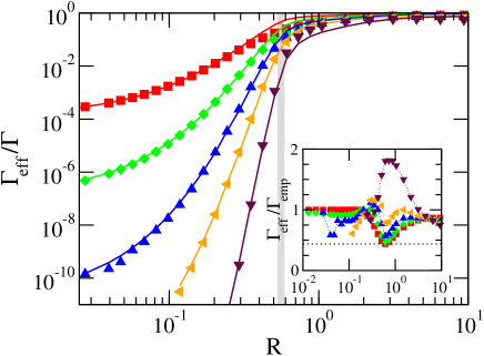
Figure 4: (Color online) The ratio $\Gamma_{\rm eff}/\Gamma$ vs $R=\Gamma/E_{\rm p}$, for $\omega_{0}/D=0.0025$ and different strengths of the electron-phonon coupling $\lambda$. Here, $\lambda$ takes the values $3$ (red), $4$ (green), $5$ (blue), $6$ (orange), and $8$ (maroon). Symbols depict the NRG data. Solid lines show the ratio $\Gamma_{\rm emp}/\Gamma$, obtained using the empirical formula $\Gamma_{\rm emp}=\Gamma\exp[-\lambda^{2}{\cal F}(R)]$ with ${\cal F}(R)$ given by the solid line in Fig. 5. The gray shaded area covers the regime where the condition $\Gamma_{\rm eff}=\omega_{0}$ is met for all values of $\lambda$ displayed. Inset: The ratio $\Gamma_{\rm eff}/\Gamma_{\rm emp}$ for all data points displayed in the main panel. The empirical formula and NRG data agree to within a factor of $2.3$ for all values of $\lambda$ and all ratios $\Gamma/E_{\rm p}$ displayed (the dotted line marks the value 0.44). NRG parameters: $\Lambda=2$, $N_{\rm s}=8000$, and $N_{\rm b}=3000$.

IV.2 Renormalized tunneling rate $\Gamma_{\rm eff}$

We begin our discussion with the renormalized tunneling rate $\Gamma_{\rm eff}$, defined by Eqs. (7) and (8) with $\chi_{c}$ evaluated for $T\to 0$. Figure 4 shows the dependence of $\Gamma_{\rm eff}$ on $\Gamma$ for $\omega_{0}/D=0.0025$ and different strengths of the electron-phonon coupling $\lambda$. As expected, the ratio $\Gamma_{\rm eff}/\Gamma$ varies by orders of magnitude upon going from small to large values of $\Gamma$ when $\lambda$ is large. For $E_{\rm p}\ll\Gamma$, one essentially recovers the bare tunneling rate $\Gamma$, while for $\Gamma\ll\omega_{0}$ there is an exponential suppression of the tunneling rate according to $\Gamma_{\rm eff}/\Gamma=e^{-\lambda^{2}}$. Remarkably, the crossover between these two limits follows an approximate scaling form, as demonstrated in Fig. 5. Plotting $\lambda^{-2}\ln(\Gamma/\Gamma_{\rm eff})$ as a function of $R=\Gamma/E_{\rm p}$ for the different values of $\lambda$, all data points approximately collapse onto a single curve. The collapse is particularly good in the range $R\lesssim 0.2$, and gradually degrades for larger values of $R$. Note that $E_{\rm p}/D$ equals $0.16$ for $\lambda=8$, hence some values of $\Gamma$ become of order the bandwidth for $R\sim 10$.

The quality of the approximate scaling form (which, as we show below, is not an exact scaling function) can be appreciated by extracting an empirical function ${\cal F}(R)$ such that ${\cal F}(R)\approx\lambda^{-2}\ln(\Gamma/\Gamma_{\rm eff})$, and comparing the calculated values of $\Gamma_{\rm eff}$ to the empirical formula

$$\Gamma_{\rm emp}=\Gamma\exp[-\lambda^{2}{\cal F}(R)].$$ (47)

The empirical formula, depicted by the solid lines in Fig. 4, well agrees with the calculated values of $\Gamma_{\rm eff}$ over many orders of magnitude. Deviations are confined to within a factor of $2.3$ (see inset of Fig. 4), which is quite remarkable considering the enormous variation in $\Gamma_{\rm eff}$ as a function of both $\lambda$ and $\Gamma$. As for the function ${\cal F}(R)$, we define it by the solid line in Fig. 5. Obviously, there is some arbitrariness in the way ${\cal F}(R)$ is fixed, particularly for $R\gtrsim 0.2$ where scaling degrades. Indeed, it is in this parameter regime that the deviations between $\Gamma_{\rm emp}$ and $\Gamma_{\rm eff}$ are typically the largest. Still, Eq. (47) provides a useful formula for the renormalized tunneling rate, successfully interpolating between the extreme adiabatic and antiadiabatic limits. Finally, we note that the condition $\Gamma_{\rm eff}=\omega_{0}$ is met for $R$ in the range $0.53<R<0.59$ (gray shaded area in Fig. 4) for all values of $\lambda$ displayed, hence the two scales remain well separated up to $R\sim 0.4$.

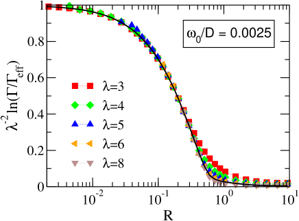
Figure 5: (Color online) The function $\lambda^{-2}\ln(\Gamma/\Gamma_{\rm eff})$ vs $R=\Gamma/E_{\rm p}$, for $\omega_{0}/D=0.0025$ and different strengths of the electron-phonon coupling $\lambda$. The solid line is an empirical curve that defines the function ${\cal F}(R)$, which is used in Fig. 4 to compute $\Gamma_{\rm emp}=\Gamma\exp[-\lambda^{2}{\cal F}(R)]$. All NRG parameters are the same as in Fig. 4.

IV.3 Extended antiadiabatic limit: Mapping onto the IRLM

Next we focus on the resonance condition $\Delta\epsilon_{d}=0$ and examine in greater detail the regime where $\Gamma_{\rm eff}\ll\omega_{0}$. For the case of interest where $1\ll\lambda$, this condition corresponds to $\Gamma\ll E_{\rm p}$, which encompasses both the antiadiabatic limit $\Gamma\ll\omega_{0}$ and an extended region where $\Gamma$ exceeds $\omega_{0}$ and yet $\Gamma_{\rm eff}\ll\omega_{0}$. As discussed in Sec. III.3, we anticipate for such couplings that the system is described at energies below $\omega_{0}$ by an effective IRLM with the tunneling amplitude $t_{\rm eff}$ and the local Coulomb repulsion $U_{\rm eff}$. Using the NRG level flow, we have confirmed this physical picture. In the intermediate energy regime $\Gamma_{\rm eff}\ll D_{N}<\omega_{0}$, the finite-size spectra consistently reduced to that of a weakly coupled IRLM, proving the validity of the extended antiadiabatic regime. The coupling constants that enter the effective Hamiltonian can be read off from the NRG spectra using the procedure outlined in Appendix B. Our results are summarized in Figs. 6 and 7.

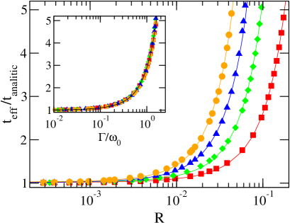
Figure 6: (Color online) The tunneling amplitude $t_{\rm eff}$ that enters the effective IRLM at energy $D_{\rm eff}/\omega_{0}=0.146$, plotted vs $R=\Gamma/E_{\rm p}$. Here $\omega_{0}/D=0.0025$, while $D_{\rm eff}$ equals $D_{N=22}$ with $\Lambda=2$. The values of $\lambda$ are $3$ (red), $4$ (green), $5$ (blue), and $6$ (orange). The remaining NRG parameters are $N_{\rm s}=8000$ and $N_{\rm b}=3000$. For clarity, $t_{\rm eff}$ was normalized by $t_{\rm analytic}=t\,e^{-\lambda^{2}/2}$, which is the effective tunneling amplitude obtained for $\Gamma\ll\omega_{0}$. Inset: A scaling plot of $t_{\rm eff}/t_{\rm analytic}$ vs $\Gamma/\omega_{0}$. The solid line shows the parabola $f(x)=1+0.9x+x^{2}$.

Figure 6 displays the effective tunneling amplitude $t_{\rm eff}$ at energy $D_{\rm eff}/\omega_{0}=0.146$ for several values of $\lambda=2$, $4$, $5$, and $6$. For clarity, all curves have been normalized by $t_{\rm analytic}=t\,e^{-\lambda^{2}/2}$, which accounts for the main Gaussian dependence of $t_{\rm eff}$ on $\lambda$. As can be seen in the inset, all data points for $t_{\rm eff}/t_{\rm analytic}$ collapse onto a single curve when plotted versus $\Gamma/\omega_{0}$, at least for values of $\Gamma$ up to a few times $\omega_{0}$. Thus, the effective tunneling amplitude acquires the empirical scaling form

$$t_{\rm eff}=t\cdot\exp\!\left[-\frac{\lambda^{2}}{2}\right]f(\Gamma/\omega_{0}),$$ (48)

where $f(x)$ is well fitted by the parabola $f(x)\approx 1+0.9x+x^{2}$ (depicted by the full line in the inset of Fig. 6). Three points are noteworthy. First, $t_{\rm eff}$ grows quite rapidly with $\Gamma/\omega_{0}$, increasing by a factor of $5$ in the limited range covered by the inset of Fig. 6. Second, given the apparent scaling of $t_{\rm eff}/t_{\rm analytic}$ with $\Gamma/\omega_{0}$, it is evident that the ratio $\Gamma_{\rm eff}/\Gamma$ cannot be an exclusive function of $\Gamma/E_{\rm p}$ as suggested by the scaling plot of Fig. 5. Lastly, we cannot reliably extract $t_{\rm eff}$ for larger values of $\Gamma/\omega_{0}$ since $t_{\rm eff}$ and $U_{\rm eff}$ no longer represent well-separated energy scales (for technical details, see Appendix B).

The effective Coulomb repulsion $U_{\rm eff}$ at energy $D_{\rm eff}/\omega_{0}=0.146$ is shown in turn in Fig. 7, after division by its asymptotic weak-tunneling form $U_{\rm analytic}=2R/(\pi\rho_{0})$ [see Eq. (27) with $1\ll\lambda$]. Note that in contrast to $t_{\rm eff}$, which becomes numerically inaccessible for $8\lesssim\lambda$, the effective Coulomb repulsion $U_{\rm eff}$ can be accurately computed for values of $\lambda$ well above $10$. Surprisingly, the weak-tunneling expression that was derived strictly speaking for $\Gamma\ll\omega_{0}$ remains quite accurate (to within 10%) even for $\Gamma/\omega_{0}$ as large as $100$ when $\lambda=20$. Hence, the main source of $\Gamma$ dependence stems from $U_{\rm analytic}$ which scales as $\Gamma/E_{\rm p}$. Similar to $t_{\rm eff}/t_{\rm analytic}$ also $U_{\rm eff}/U_{\rm analytic}$ appears to follow an approximate scaling form, this time with the scaling variable $\Gamma/(\lambda^{2.5}\omega_{0})$ (see inset of Fig. 7). However, the quality of the data collapse and the variation in $U_{\rm eff}/U_{\rm analytic}$ are far more restricted than for $t_{\rm eff}/t_{\rm analytic}$.

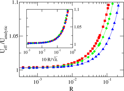
Figure 7: (Color online) The local Coulomb repulsion $U_{\rm eff}$ that enters the effective IRLM at energy $D_{\rm eff}/\omega_{0}=0.146$, plotted vs $R=\Gamma/E_{\rm p}$. The values of $\lambda$ are $5$ (red), $10$ (green), and $20$ (blue). All other parameters are the same as in Fig. 6. For clarity, $U_{\rm eff}$ was normalized by $U_{\rm analytic}=2R/(\pi\rho_{0})$, which is the effective Coulomb repulsion for $\Gamma\ll\omega_{0}$. Inset: A scaling plot of $U_{\rm eff}/U_{\rm analytic}$ versus $R/\sqrt{\lambda}$.

From the discussion above it is clear that the regimes $\Gamma\ll\omega_{0}$ and $\omega_{0}<\Gamma\ll E_{\rm p}$ share the same qualitative physics, both being described by the same IRLM at energies below $\omega_{0}$. The distinction between the two regimes is mainly quantitative, as encoded in the effective model parameters $t_{\rm eff}$ and $U_{\rm eff}$. The rather rapid departure of $t_{\rm eff}$ from its asymptotic weak-tunneling form $t\,e^{-\lambda^{2}/2}$ reflects its extreme sensitivity to even small deformations of the polaronic mode.

IV.4 Charging of the level

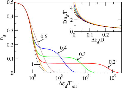
Figure 8: (Color online) The level occupancy $n_{d}$ vs $\Delta\epsilon_{d}=\epsilon_{d}-\epsilon_{d}^{\ast}>0$, for $\omega_{0}/D=0.0025$, $T\to 0$, $\lambda=6$, and different values of $R=\Gamma/E_{\rm p}$ (indicated by arrows). The level occupancy in the complementary regime $\Delta\epsilon_{d}<0$ is obtained from the symmetry relation of Eq. (6). With increasing $\Gamma\geq E_{\rm p}$, charging of the level approaches the conventional noninteracting curve, depicted by the dotted line. With decreasing $\Gamma<E_{\rm p}$, the noninteracting shape rapidly deforms into a double-step structure governed by distinct mechanisms for $\Delta\epsilon_{d}\lesssim\Gamma_{\rm eff}$ and $\Gamma_{\rm eff}\ll\Delta\epsilon_{d}$. For $\Delta\epsilon_{d}\lesssim\Gamma_{\rm eff}$, one recovers a strongly renormalized noninteracting form with $\Gamma\to\Gamma_{\rm eff}$. For $\Gamma_{\rm eff}\ll\Delta\epsilon_{d}$, charging is well described by a simple perturbative expansion in $t$. This is demonstrated in the inset, where each of the occupancies of the main panel is compared to the perturbative expression of Eq. (33) (dashed line). NRG parameters: $\Lambda=2$, $N_{\rm s}=4000$, and $N_{\rm b}=1600$.

Up until now, our discussion was restricted to $\Delta\epsilon_{d}=0$. Next we consider nonzero detuning and examine the charging properties of the $d$ level. Besides being of interest on its own right, the charge of the level is intimately related at $T=0$ to the conductance of the molecular bridge depicted schematically in Fig. 11. We address the latter setup in detail in Sec. V.

Figure 8 shows the level occupancy $n_{d}$ versus $\Delta\epsilon_{d}>0$, for $T\to 0$ and $\lambda=6$. The level occupancy in the complementary regime $\Delta\epsilon_{d}<0$ is obtained from the symmetry relation of Eq. (6). With increasing $\Gamma\geq E_{\rm p}$, charging of the level approaches the conventional noninteracting curve, depicted by the dotted line. With decreasing $\Gamma<E_{\rm p}$, the noninteracting shape rapidly deforms into a charging curve governed by two distinct mechanisms: (i) a strongly renormalized noninteracting form with $\Gamma\to\Gamma_{\rm eff}$, applicable up to $\Delta\epsilon_{d}\sim\Gamma_{\rm eff}$, and (ii) a simple perturbative expansion in $t$, applicable for $\Gamma_{\rm eff}\ll\Delta\epsilon_{d}$. The latter mechanism is demonstrated in the inset, where each of the curves of the main panel is compared to the perturbative expression of Eq. (33) (dashed line).

The combination of these two mechanisms gives rise to a distinctive shoulder in $n_{d}$, which interpolates between the limits where $\Delta\epsilon_{d}\sim\Gamma_{\rm eff}$ and $\Delta\epsilon_{d}\sim\Gamma$. The height of the shoulder decreases with decreasing $\Gamma$, approaching $\Gamma/(\pi E_{\rm p})$ when $\Gamma\ll E_{\rm p}$. This result can be understood from the fact that the summation over $n$ in Eq. (33) samples mainly the regime where $n\sim\lambda^{2}$ when $\lambda$ is large, hence the denominator $\Delta\epsilon_{d}+n\omega_{0}$ is effectively replaced with $\Delta\epsilon_{d}+\lambda^{2}\omega_{0}\approx E_{\rm p}$. This argumentation breaks down as $\Delta\epsilon_{d}$ approaches $\Gamma_{\rm eff}$, when higher order terms become exceedingly more important. Another effect of decreasing $\Gamma$ is the opening of an exponential separation between $\Gamma$ and $\Gamma_{\rm eff}$, which sets the lateral extent of the shoulder when plotted versus $\Delta\epsilon_{d}/\Gamma_{\rm eff}$. For example, $\Gamma$ and $\Gamma_{\rm eff}$ are separated by one order of magnitude for $R=0.6$, which is insufficient for a fully developed shoulder to be seen.

IV.5 Phononic distribution

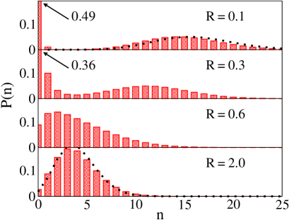
Figure 9: (Color online) The phonon distribution function $P(n)=\left<|n\rangle\langle n|\right>$, for $\omega_{0}/D=0.0025$, $\lambda=4$, $N_{0}=0$, $T\to 0$, and different values of $R=\Gamma/E_{\rm p}$. The detuning energy $\Delta\epsilon_{d}$ is set to zero such that the electronic level is half filled. For $R\ll 1$, exemplified by $R=0.1$ in the upper panel, the distribution function $P(n)$ approaches the double-peak structure of Eq. (41), depicted by the dotted line. In the opposite limit where $R$ is large, exemplified by $R=2$ in the lower panel, the distribution function $P(n)$ approaches the single-peak structure of Eq. (37), displayed by the dotted line. NRG parameters: $\Lambda=2$, $N_{\rm s}=4000$, and $N_{\rm b}=1600$.

To gain direct information on the state of the phonon, we next consider the phonon distribution function $P(n)$, defined in Eq. (35). Figure 9 depicts $P(n)$ for $T\to 0$ using $\lambda=4$, $N_{0}=0$, and different values of $R=\Gamma/E_{\rm p}$. The detuning energy $\Delta\epsilon_{d}$ (which itself depends on $N_{0}$ through $\epsilon_{d}^{\ast}$) is set to zero, corresponding to resonance condition. For small values of $\Gamma$, exemplified by $R=0.1$ in the upper panel, the distribution function $P(n)$ approaches the double-peak structure of Eq. (41), which is plotted for comparison by the dotted line. Although $\Gamma$ equals $1.6\omega_{0}$ in this case, the phonon distribution function remains well described by the antiadiabatic result which applies, strictly speaking, to $\Gamma\ll\omega_{0}$. Physically this means that the degree of undressing of the polaron is rather small for this particular value of $\Gamma$. A qualitative change in the profile of $P(n)$ takes place upon going from $R=0.3$ to $R=0.6$, marking the progressive undressing of the polaron. Finally for large $\Gamma$, exemplified by $R=2$ in the lower panel, the distribution function $P(n)$ approaches the single-peak structure of Eq. (37), which is plotted for comparison by the dotted line. As discussed in Sec. III.5, the phonon is too slow to track the individual tunneling events in this limit, hence it samples only the average displacement $\lambda\langle\hat{n}_{d}\rangle=\lambda/2$.

A useful perspective on the phononic state is provided by varying the reference charge $N_{0}$ of the electronic level. As discussed in Sec. II, $N_{0}$ can be eliminated from the Hamiltonian of Eq. (1) by simply shifting the bosonic mode according to $\hat{B}=b-\lambda N_{0}$. If the level energy $\epsilon_{d}$ is simultaneously adjusted such that $\Delta\epsilon_{d}=\epsilon_{d}-\lambda^{2}\omega_{0}(1-2N_{0})$ is held fixed, then the variation of $N_{0}$ has no effect on the low-energy spectrum of the Hamiltonian. Nevertheless, the low-energy state of the system does vary with $N_{0}$, as can be seen from the case where the $\hat{B}$ boson occupies a pure coherent state. If $\hat{B}$ resides in the coherent state $|z\rangle$, then the $b$ phonon occupies the shifted coherent state $|z+\lambda N_{0}\rangle$. In other terms, one can continuously vary the coherent state that $b$ occupies by tuning $N_{0}$ while holding $\Delta\epsilon_{d}$ fixed. This strategy can be used not only to expose a pure coherent state, but also to diagnose a superposition involving a small number of coherent states of the type often used in variational calculations.

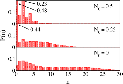
Figure 10: (Color online) The phonon distribution function $P(n)=\left<|n\rangle\langle n|\right>$, for $\omega_{0}/D=0.0025$, $\lambda=6$, $R=\Gamma/E_{\rm p}=0.5$, $T\to 0$, and different values of $N_{0}$. The detuning energy $\Delta\epsilon_{d}$ is held fixed at zero for all values of $N_{0}$, such that the electronic level is half filled. NRG parameters: $\Lambda=2$, $N_{\rm s}=4000$, and $N_{\rm b}=1600$.

Figure 10 displays the evolution of the phonon distribution function with increasing $N_{0}$, for $\lambda=6$ and fixed $\Delta\epsilon_{d}=0$. The ratio $\Gamma/E_{\rm p}=0.5$ is tuned to the middle of the crossover regime, such that the system is well removed from the extreme adiabatic and antiadiabatic limits. As can be seen, $P(n)$ evolves in a rather complicated manner upon going from $N_{0}=0$ to $N_{0}=0.5$. Initially, there are two rather broad and smooth humps for $N_{0}=0$. Upon increasing $N_{0}$, the phonon distribution function narrows considerably, developing multiple sharp peaks by the time $N_{0}=0.5$. Indeed, $3$ clear maxima are visible at $n=0$, $2$, and $4$ when $N_{0}=0.5$, indicating that at least three independent coherent states significantly contribute to the low-energy state of the system. We have not succeeded in reproducing this multiple-peak structure for $N_{0}=0.5$ (let alone the entire collection of distributions for the different values of $N_{0}$) by employing a simple superposition of just a few coherent states. Given the sharpness of the peaks found at even values of $n$, it is clear that the low-energy state of the system can not be well represented using just one or two coherent states. This sets a stringent constraint on variational treatments of the crossover regime when $\lambda$ is large.

V Conductance of a molecular bridge

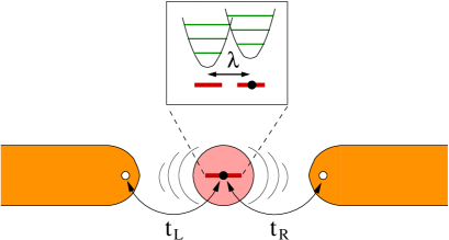
Figure 11: (Color online) Schematic description of a molecular bridge, where a single molecule is trapped between two leads.

Our discussion thus far has focused on thermodynamic quantities, which are difficult to measure for a single molecule. Of particular interest are transport properties of molecular devices of the type displayed schematically in Fig. 11, where a single molecule is trapped between two leads. Continuing with spinless fermions, we model such a molecular bridge by the Hamiltonian

$${\cal H} =\sum_{k,\alpha}\epsilon_{k}c^{\dagger}_{k\alpha}c_{k\alpha}+\sum_{\alpha}\frac{t_{\alpha}}{\sqrt{N}}\sum_{k}\left\{d^{\dagger}c_{k\alpha}+{\rm H.c.}\right\}$$

$$+\epsilon_{d}d^{\dagger}d+\omega_{0}b^{\dagger}b+\lambda\omega_{0}\!\left(d^{\dagger}d-N_{0}\right)\!\left(b^{\dagger}+b\right),$$ (49)

where $\alpha=L,R$ labels the left/right lead. Here, $c^{\dagger}_{k\alpha}$ creates a conduction electron with momentum $k$ in lead $\alpha$, while $t_{\alpha}$ is the tunneling matrix element between the electronic level and the Wannier state closest to the molecule in lead $\alpha$. For convenience we take the number of lattice sites $N$ to be the same in both leads, although this condition can easily be relaxed.

In equilibrium, the two-lead Hamiltonian of Eq. (49) is equivalent to the single-band model of Eq. (1). This stems from the fact that the localized level couples solely to the “bonding” combination

$$c^{\dagger}_{+k}=\frac{t_{L}}{\sqrt{t_{L}^{2}+t_{R}^{2}}}\,c^{\dagger}_{kL}+\frac{t_{R}}{\sqrt{t_{L}^{2}+t_{R}^{2}}}\,c^{\dagger}_{kR},$$ (50)

while the “anti-bonding” combination

$$c^{\dagger}_{-k}=\frac{t_{R}}{\sqrt{t_{L}^{2}+t_{R}^{2}}}\,c^{\dagger}_{kL}-\frac{t_{L}}{\sqrt{t_{L}^{2}+t_{R}^{2}}}\,c^{\dagger}_{kR}$$ (51)

is decoupled from the level. Inasmuch as impurity-related quantities are concerned, one can omit then the “anti-bonding” band altogether, to be left with the single-band Hamiltonian of Eq. (1) where $t=\sqrt{t_{L}^{2}+t_{R}^{2}}$.

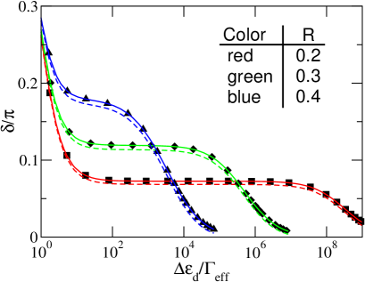
Figure 12: (Color online) The scattering phase shift $\delta$ vs the detuning energy $\Delta\epsilon_{d}$, for $\omega_{0}/D=0.0025$, $\lambda=6$, $T\to 0$, and three intermediate values of $R=\Gamma/E_{\rm p}$. Here $\Gamma=\Gamma_{L}+\Gamma_{R}$ is the total tunneling rate from the level to the two leads. Solid lines depict the phase shift $\delta/\pi$, dashed lines show the dot occupancy $n_{d}$, and the symbols show the number of displaced electrons, $\Delta N$. In accordance with the Friedel-Langreth sum rule, $\delta/\pi$ coincides with $\Delta N$, which deviates, however, from $n_{d}$. NRG parameters: $\Lambda=2$, $N_{\rm s}=4000$, and $N_{\rm b}=1600$.

The restriction to the “bonding” band is no longer complete when a finite bias is applied between the leads, since the nonequilibrium boundary condition applies to the lead electrons rather than their “bonding” and “anti-bonding” combinations. Thus, one can no longer settle with the single-band Hamiltonian of Eq. (1) for a biased junction. Fortunately, this complication can be circumvented in linear response, when the conductance can be expressed in terms of equilibrium response functions of the system. In particular, the zero-temperature conductance, $G$, is determined by the scattering phase shift of the “bonding” electrons, as follows from the Fermi-liquid ground state of the system. The zero-temperature conductance thus takes the standard form

$$G=G_{0}\sin^{2}(\delta),$$ (52)

where

$$G_{0}=\frac{e^{2}}{h}\frac{4\Gamma_{L}\Gamma_{R}}{(\Gamma_{L}+\Gamma_{R})^{2}}$$ (53)

with $\Gamma_{\alpha}=\pi\rho_{0}t_{\alpha}^{2}$ is a geometric factor encoding the degree of asymmetry in the coupling to the two leads and $\delta$ is the scattering phase shift. Generalizing the Friedel-Langreth sum rule Langreth66 to the present setting, the phase shift $\delta$ is given by

$$\delta=\pi\Delta N,$$ (54)

where $\Delta N$ is the number of displaced electrons. The latter quantity comprises two contributions: (i) occupancy of the level $n_{d}$, and (ii) the change in occupancy of the “bonding” band inflicted by the coupling to the level. In the wide-band limit only the former contribution is left, resulting in $\delta=\pi n_{d}$. However, as we show below, $\Delta N$ deviates from $n_{d}$ when the conduction-electron bandwidth is finite.

Figure 12 shows the scattering phase shift $\delta/\pi$ versus $\Delta\epsilon_{d}$, calculated directly from the NRG spectra using the standard prescription ALPC92 of Eq. (78). For comparison, we also plot the level occupancy $n_{d}$ and the number of displaced electrons $\Delta N$, which is readily computed in the NRG since the total electronic occupancy of the system is a good quantum number that is kept track of in the course of the iterative procedure. The electron-phonon coupling is set equal to $\lambda=6$, while $\Gamma=\Gamma_{L}+\Gamma_{R}$ is tuned to three intermediate values of $R=\Gamma/E_{\rm p}$ where $n_{d}$ shows a pronounced shoulder.

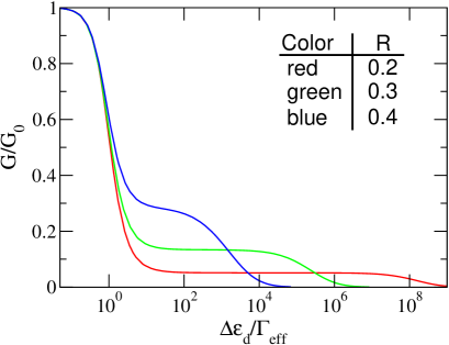
Figure 13: (Color online) The zero-temperature conductance $G$ vs the detuning energy $\Delta\epsilon_{d}$, plotted for the same model and NRG parameters as in Fig. 12. Here $G_{0}$ is a geometric factor specified in Eq. (53), encoding the asymmetry of the tunnel junction. The characteristic shoulder in $n_{d}$ translates to a similar shoulder in $G/G_{0}$, providing a distinct experimental fingerprint of phonon-assisted tunneling when the electron-phonon coupling is strong.

While $\delta/\pi$ and $\Delta N$ are indistinguishable to within numerical accuracy, there is a small but consistent deviation from $n_{d}$, particularly along the characteristic shoulder in $n_{d}$. The difference between $\Delta N$ and $n_{d}$ appears to somewhat increase upon going from $R=0.2$ to $0.4$, and disappears for $\Delta\epsilon_{d}\to 0$ (not shown). This latter behavior is to be expected since $\delta/\pi$, $\Delta N$, and $n_{d}$ are all pinned to $1/2$ by particle-hole symmetry when $\Delta\epsilon_{d}=0$.

The corresponding zero-temperature conductance is shown in turn in Fig. 13 as a function of the detuning energy $\Delta\epsilon_{d}$. Note that the conductance is an even function of $\Delta\epsilon_{d}$, as follows from the particle-hole transformation of Eq. (3). Hence only the regime $\Delta\epsilon_{d}>0$ is displayed. The characteristic shoulder in $n_{d}$ translates to a similar shoulder in $G/G_{0}$, which is further pushed down in magnitude due to the quadratic dependence on $\sin(\delta)$. Experimentally, $\Delta\epsilon_{d}$ can be tuned using a suitable gate voltage, giving rise to characteristic shoulders in the conductance as a function of gate voltage. These shoulders, which are quite unique in the context of tunneling through confined nanostructures, provide a distinct experimental fingerprint of phonon-assisted tunneling when the electron-phonon coupling is strong.

VI Summary

Focusing on strong electron-phonon interactions, $1\ll\lambda$, we presented a comprehensive study of the crossover from the antiadiabatic to the adiabatic regime of phonon-assisted tunneling in the framework of a minimal model for molecular devices: a resonant level coupled by displacement to a single localized vibrational mode. Our main findings are as follows.

1. In contrast to common lore, the crossover from the polaronic physics of the antiadiabatic limit to the perturbative physics of the adiabatic regime is governed primarily by the polaronic shift $E_{\rm p}=\lambda^{2}\omega_{0}$ rather than the phonon frequency $\omega_{0}$. In particular, the perturbative adiabatic limit is approached only as the bare hopping rate $\Gamma$ exceeds the polaronic shift, leaving an extended window of couplings where $\Gamma$ well exceeds the phonon frequency and yet the physics is basically that of the antiadiabatic regime.

2. Throughout the traditional and the extended antiadiabatic regimes, the effective low-energy Hamiltonian at energies below $\omega_{0}$ is the purely fermionic IRLM, which depends at resonance on two parameters only: $t_{\rm eff}$ and $U_{\rm eff}$. The effective tunneling amplitude $t_{\rm eff}$ obeys the empirical scaling form of Eq. (48), at least up to values of $\Gamma$ several times larger than $\omega_{0}$, while $U_{\rm eff}$ is well approximated by Eq. (26) for much of the extended antiadiabatic regime.

3. Although $\Gamma_{\rm eff}$ varies by many orders of magnitude as a function of $\lambda$ and $R=\Gamma/E_{\rm p}$, it is rather well described for all parameter regimes by the empirical formula of Eq. (47), which depends on a single scaling function ${\cal F}(R)$. Our proposal for ${\cal F}(R)$ is given by the solid line in Fig. 5, although this choice can possibly by further optimized.

4. Charging properties are governed by two distinct mechanisms at the extended antiadiabatic and into the crossover regime. At small detuning, $\Delta\epsilon_{d}\lesssim\Gamma_{\rm eff}$, the level occupancy $n_{d}$ follows a strongly renormalized noninteracting form with $\Gamma\to\Gamma_{\rm eff}$. By contrast, a simple perturbative expansion in $t$ applies for $\Gamma_{\rm eff}\ll\Delta\epsilon_{d}$, giving rise to a characteristic shoulder in $n_{d}$ and in the low-temperature conductance of a molecular junction as a function of gate voltage.

Our scenario for the crossover from the antiadiabatic to the adiabatic regime is summarized in Fig. 1, where we have merged the traditional and the extended antiadiabatic regimes on the basis the two are qualitatively the same.

This study was devoted to thermodynamic properties, for which a rather complete picture was provided. However, the question of real-time dynamics remains largely open. Particularly, does $\tau_{\rm p}=1/E_{\rm p}$ show up as a new time scale in the dynamics? As could be anticipated, $\tau_{\rm p}$ plays no role deep in the adiabatic regime, when $E_{\rm p}\ll\Gamma$. Indeed, as recently shown for different scenarios of quench and driven dynamics, VSA12 only three time scales are involved in this limit: the dwell time $\tau_{\rm dwell}=1/\Gamma$, the period of oscillations $\tau_{\rm osc}=2\pi/\omega_{\rm eff}$ with the softened frequency of Eq. (21), and the phonon damping time $\tau_{\rm damp}=\pi\Gamma^{2}/(\lambda^{2}\omega_{0}^{3})$, extracted from the imaginary part of Eq. (20). Other perturbative RS2009 and numerical Muehlbacher-rabani-2008 ; Thoss-2011 ; Thoss-2012 studies of real-time dynamics have focused primarily on the build up of the current in a biased two-lead setting, revealing rich behavior. Most notably, a significant dependence on the initial state was reported in Ref. Thoss-2012, up to times far exceeding $\tau_{\rm dwell}$, suggesting the existence of another, much longer time scale whose origin is not quite clear. We note in passing that the parameter set referred to as adiabatic in the latter study corresponds in our notation to $\lambda=8$ and $R=1/8$, which actually falls in the extended antiadiabatic regime. This may suggest the possible relevance at long times of a strongly renormalized tunneling rate akin to $\Gamma_{\rm eff}$. Clearly the understanding of real-time dynamics in molecular devices is a timely and challenging task that deserves further investigation.

Appendix A Schrieffer-Wolff-type transformation for $\Gamma\ll\omega_{0}$

In this Appendix, we describe the Schrieffer-Wolff-type transformation that maps the Hamiltonian of Eq. (22) onto the IRLM Hamiltonian of Eq. (24), with the coupling constants $t_{\rm eff}$ and $U_{\rm eff}$ specified in Eqs. (25) and (26), respectively. As emphasized in the main text, the mapping applies to $\Gamma\ll\omega_{0}$, when a single-step elimination of all excitation energies exceeding $\omega_{0}$ is sufficient. The mapping is further restricted to temperatures below $\omega_{0}$, when the (transformed) phonon is frozen in its unperturbed ground-state configuration $b^{\dagger}b=0$.

Following Schrieffer and Wolff, SW66 we seek a canonical transformation

$${\cal H}_{\rm S}=e^{S}{\cal H}^{\prime}e^{-S}$$ (55)

with a suitable anti-Hermitian operator $S$ such that the low-energy subspace is decoupled to order $t^{2}$ from all excited phononic states and all single-particle conduction-electron excitations with energy $|\epsilon_{k}|>\omega_{0}$ (whether particle or hole). To this end, we introduce two complementary projection operators, $P$ and $Q=1-P$, where $P$ projects onto the low-energy subspace with $b^{\dagger}b=0$ and no single-particle conduction-electron excitations whose energy exceeds $\omega_{0}$. In other terms, all conduction-electron modes with energy $\epsilon_{k}<-\omega_{0}$ ($\omega_{0}<\epsilon_{k}$) are strictly occupied (unoccupied) within the subspace defined by $P$. The Hamiltonian ${\cal H}^{\prime}$ is then divided into an “unperturbed” part ${\cal H}^{\prime}_{0}$ and a “perturbation” ${\cal H}^{\prime}_{1}$, where

$${\cal H}^{\prime}_{0}=P{\cal H}^{\prime}P+Q{\cal H}^{\prime}Q$$ (56)

and

$${\cal H}^{\prime}_{1}=P{\cal H}^{\prime}Q+Q{\cal H}^{\prime}P.$$ (57)

Explicitly, ${\cal H}^{\prime}_{0}$ takes the form

$${\cal H}^{\prime}_{0} ={\cal H}_{0}+\frac{t}{\sqrt{N}}e^{-\lambda^{2}/2}\sum_{k}^{\rm restric}\left\{d^{\dagger}c_{k}+{\rm H.c.}\right\}|0\rangle\langle 0|P$$

$$+\frac{t}{\sqrt{N}}Q\sum_{k}\left\{e^{\lambda(b^{\dagger}-b)}d^{\dagger}c_{k}+{\rm H.c.}\right\}Q$$ (58)

with

$${\cal H}_{0}=\sum_{k}\epsilon_{k}c^{\dagger}_{k}c_{k}+\omega_{0}b^{\dagger}b,$$ (59)

while ${\cal H}^{\prime}_{1}$ is given by ${\cal H}^{\prime}_{1}=\tilde{\cal H}^{\prime}_{1}P+{\rm H.c.}$ with

$$\tilde{\cal H}^{\prime}_{1} =\frac{t}{\sqrt{N}}\sum_{n>0}\sum_{k}\left[U^{-}_{n}c^{\dagger}_{k}d+U^{+}_{n}d^{\dagger}c_{k}\right]|n\rangle\langle 0|$$

$$+\frac{t}{\sqrt{N}}e^{-\lambda^{2}/2}\left[\sum_{k}^{\rm elec}c^{\dagger}_{k}d+\sum_{q}^{\rm hole}d^{\dagger}c_{q}\right]|0\rangle\langle 0|$$ (60)

and

$$U^{\pm}_{n}=e^{-\lambda^{2}/2}\frac{(\pm\lambda)^{n}}{\sqrt{n!}}.$$ (61)

Here the symbols $\sum_{k}^{\rm elec}$ and $\sum_{q}^{\rm hole}$ come to indicate that the summations over $k$ and $q$ are restricted to momenta such that $\epsilon_{k}>\omega_{0}$ and $\epsilon_{q}<-\omega_{0}$, respectively.

Using the formal expansion

$${\cal H}_{\rm S}={\cal H}^{\prime}_{0}+{\cal H}^{\prime}_{1}+[S,{\cal H}^{\prime}_{0}]+[S,{\cal H}^{\prime}_{1}]+\frac{1}{2}[S,[S,{\cal H}^{\prime}_{0}]]+\ldots$$ (62)

and anticipating that $S$ is proportional to $t$ at leading order (as will shortly be seen), one can group the different terms in Eq. (62) according to powers in $t$. The requirement that no coupling is left to order $t^{2}$ between the excited and low-energy subspaces is satisfied by demanding that

$${\cal H}^{\prime}_{1}+[S,{\cal H}^{\prime}_{0}]={\cal O}(t^{3}),$$ (63)

resulting in

$${\cal H}_{\rm S}={\cal H}^{\prime}_{0}+\frac{1}{2}[S,{\cal H}^{\prime}_{1}]+{\cal O}(t^{3}).$$ (64)

Equation (63) has the formal solution

$$S=-\frac{1}{{\cal L}^{\prime}_{0}}{\cal H}^{\prime}_{1}+{\cal O}(t^{3}),$$ (65)

where ${\cal L}^{\prime}_{0}$ is the Liouville operator defined by ${\cal L}^{\prime}_{0}\hat{O}=[\hat{O},{\cal H}^{\prime}_{0}]$. Since ${\cal H}^{\prime}_{1}$ is proportional to $t$, it is clear that $S$ has a leading linear dependence on $t$, as we have assumed. The anti-Hermitian operator $S$ does contain, however, additional higher order terms in $t$, which stem from the fact that ${\cal H}^{\prime}_{0}$ (and thus ${\cal L}^{\prime}_{0}$) includes components linear in $t$ [see Eq. (58)]. Denoting the linear-order component of $S$ by $S^{(1)}$, the latter is computed by substituting ${\cal H}^{\prime}_{0}\to{\cal H}_{0}$, corresponding to setting ${\cal L}^{\prime}_{0}\to{\cal L}_{0}$ with ${\cal L}_{0}\hat{O}=[\hat{O},{\cal H}_{0}]$ in Eq. (65). Using ${\cal H}^{\prime}_{1}$ of Eq. (60), this yields the explicit expression

$$S^{(1)}=\tilde{S}P-{\rm H.c.}$$ (66)

with

$$\tilde{S} =\frac{t}{\sqrt{N}}\sum_{n>0}\sum_{k}\left[c^{\dagger}_{k}d\frac{U^{-}_{n}}{\epsilon_{k}+n\omega_{0}}+d^{\dagger}c_{k}\frac{U^{+}_{n}}{n\omega_{0}-\epsilon_{k}}\right]|n\rangle\langle 0|$$

$$+\frac{t}{\sqrt{N}}e^{-\lambda^{2}/2}\left[\sum_{k}^{\rm elec}\frac{1}{\epsilon_{k}}c^{\dagger}_{k}d-\sum_{q}^{\rm hole}\frac{1}{\epsilon_{q}}d^{\dagger}c_{q}\right]|0\rangle\langle 0|.$$ (67)

To obtain ${\cal H}_{\rm S}$ up to second order in $t$, it suffices to replace $S$ in Eq. (64) with $S^{(1)}$ of Eqs. (66) and (67). Carrying out the commutator in Eq. (64), projecting the result onto the $b^{\dagger}b=0$ subspace, and restricting the band to $|\epsilon_{k}|<\omega_{0}$, one arrives to order $t^{2}$ at the effective low-energy Hamiltonian of Eq. (24) with the coupling constants specified in Eqs. (25) and (26).

Two comments should be made about the derivation of the effective Hamiltonian of Eq. (24). First, we have explicitly assumed a particle-hole symmetric band. Second, we have neglected $\epsilon_{k}$ in the denominators on the first line of Eq. (67), on the premise that $|\epsilon_{k}|$ is small as compared to the new ultraviolet cutoff energy $\omega_{0}$.

Appendix B Extracting the couplings of the effective IRLM Hamiltonian

As discussed in the main text, the Hamiltonian of Eq. (1) with $1\ll\lambda$ and $\Gamma\ll E_{\rm p}$ can be described at energies below $\omega_{0}$ by an effective IRLM. For $\Delta\epsilon_{d}=0$, the case considered hereafter, particle-hole symmetry restricts the number model parameters in the IRLM to two: the tunneling amplitude $t_{\rm eff}$ and the local Coulomb repulsion $U_{\rm eff}$. In this Appendix, we describe in detail how these model parameters can be extracted using the NRG. The analysis relies on certain characteristics, exposed below, of the finite-size spectrum of the IRLM near the free-impurity fixed point, $t_{\rm eff}=U_{\rm eff}=0$.

Energy level	Quantum numbers	Hopping matrix
($\Lambda=2$)	$(Q_{d},Q_{c})$	element to
0	$(-1,0)$	—
	$(+1,0)$	—
0.4916	$(-1,-2)$	—
	$(+1,-2)$	—
	$(-1,+2)$	—
	$(+1,+2)$	—
0.9832	$(-1,0)$	—
	$(+1,0)$	—

Table 1: Finite-size NRG spectrum at the noninteracting free-impurity fixed point $t=U=0$, for $\Lambda=2$ and odd iteration number $N$. The left column specifies the dimensionless NRG energies. The corresponding quantum numbers, $Q_{d}$ and $Q_{c}$, are listed in the central column, while the right-hand-side column indicates degenerate eigenstates that are connect to the designated state with a nonzero hopping matrix element once a finite $t$ is switched on.

In our analysis we shall use the IRLM in its following representation

$${\cal H} = \sum_{k}\epsilon_{k}c^{\dagger}_{k}c_{k}+\frac{t}{\sqrt{N_{k}}}\sum_{k}\left\{d^{\dagger}c_{k}+{\rm H.c.}\right\}$$ (68)

$$+ \frac{U}{N_{k}}\bigl{(}d^{\dagger}d-1/2\bigr{)}\sum_{k,k^{\prime}}:\!c^{\dagger}_{k}c_{k^{\prime}}\!\!:\ ,$$

where $N_{k}$ is the number of $k$ points that are summed over. This form of the Hamiltonian differs from that of Eq. (24) in the normalization factors multiplying $t$ and $U$. In Eq. (24), the summations over the momenta are restricted to $N^{\prime}<N$ values of $k$, hence the conversion between $(t_{\rm eff},U_{\rm eff})$ and $(t,U)$ reads as

$$t=t_{\rm eff}\sqrt{\frac{N^{\prime}}{N}}\;\;,\;\;\;\;\;U=U_{\rm eff}\frac{N^{\prime}}{N}.$$ (69)

For the linear dispersion considered here, the ratio $N^{\prime}/N$ equals $D_{\rm eff}/D$, where $D_{\rm eff}\sim\omega_{0}$ is the effective bandwidth in the Hamiltonian of Eq. (24) and $D$ is the full bandwidth pertaining to the original electron-phonon Hamiltonian of Eq. (1). Thus, the conversion between the corresponding coupling constants becomes

$$t=t_{\rm eff}\sqrt{\frac{D_{\rm eff}}{D}}\;\;,\;\;\;\;\;U=U_{\rm eff}\frac{D_{\rm eff}}{D},$$ (70)

which is naturally accounted for, as we shall see, in the NRG.

B.1 Finite-size spectrum of the IRLM near the free-impurity fixed point

B.1.1 Fixed-point spectrum for $t=U=0$

Consider first the noninteracting free-impurity fixed point of the IRLM with $t=U=0$. Since the impurity level is decoupled from the band, the fixed-point spectrum is simply that of a free symmetric band, with an extra degeneracy of two due to the impurity level which can be either empty or full. Thus, the ground state is doubly degenerate for odd NRG iterations $N$, and four-fold degenerate for even iterations. The corresponding eigenstates are conveniently labeled by a pair of numbers

$$Q_{d}=2d^{\dagger}d-1$$ (71)

and

$$Q_{c}=\sum_{n=0}^{N}\bigl{[}2f^{\dagger}_{n}f_{n}-1\bigr{]},$$ (72)

which serve as good quantum numbers for zero tunneling (only their sum $Q_{d}+Q_{c}$ is conserved for nonzero $t$). The two degenerate ground states for odd $N$ correspond to $(Q_{d},Q_{c})=(\pm 1,0)$, while the four degenerate ground states for even $N$ are labeled by $(Q_{d},Q_{c})=(\pm 1,\pm 1)$. The extra two-fold degeneracy for even $N$ stems from the presence of a conduction-electron mode that lies exactly at the Fermi level. The fixed-point spectra for odd and even iterations are listed in Tables 1 and 2 up to the second excitation energy.

Energy level	Quantum numbers	Hopping matrix
($\Lambda=2$)	$(Q_{d},Q_{c})$	element to
0	$(-1,-1)$	—
	$(+1,-1)$	$(-1,+1)$
	$(-1,+1)$	$(+1,-1)$
	$(+1,+1)$	—
0.9723	$(-1,-3)$	—
	$(+1,-3)$	$(-1,-1)$
	$(-1,-1)$	$(+1,-3)$
	$(+1,-1)$	—
	$(-1,+1)$	—
	$(+1,+1)$	$(-1,+3)$
	$(-1,+3)$	$(+1,+1)$
	$(+1,+3)$	—
1.9446	$(-1,-1)$	—
	$(+1,-1)$	$(-1,+1)$
	$(-1,+1)$	$(+1,-1)$
	$(+1,+1)$	—

Table 2: Same as Table 1 for even iteration number $N$.

B.1.2 Fixed-point spectrum for $t=0$ and $U\neq 0$

A small but finite $U$ lifts certain degeneracies of the $U=0$ spectrum while maintaining the same pair of quantum numbers $(Q_{d},Q_{c})$. In particular, the ground-state quartet for even $N$ is split into two doublets, each composed of two particle-hole-symmetric states. The order of doublets discloses the sign of $U$. When $U>0$, the states labeled by $(+1,-1)$ and $(-1,+1)$ [$(+1,+1)$ and $(-1,-1)$] form the ground-state [excited] doublet, while the order is reversed for $U<0$. The magnitude of $U$ can be deduced in turn from a standard phase-shift analysis ALPC92 (see below), which requires identification of the elementary particle, hole, and particle-hole excitations. For $U>0$ and even $N$, these are given by the excitation energies $\eta_{+}$, $\eta_{-}$, and $2\eta_{0}$ of the $Q_{d}=1$ sector, depicted in the middle panels of Fig. 14. In the $Q_{d}=-1$ sector the elementary particle and hole excitations are interchanged, reflecting a reversal in sign of the scattering potential experienced by the band electrons when the level is empty.

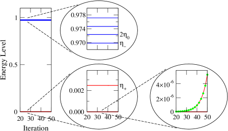
Figure 14: (Color online) Finite-size spectrum of the IRLM near the free-impurity fixed point, for $U/D=0.01$, $t/D=10^{-9}$, $\Lambda=2$, and even iterations $N$. A nonzero $U$ lifts the four-fold and eight-fold degeneracies of the ground state and the first excitation energy, respectively, splitting them into distinct doublets (middle two panels). An infinitesimal $t$ further splits some of the doublets. In particular, the ground-state doublet is split according to $\gamma(t/D)\Lambda^{N(1+\alpha)/4}$ (right panel, green dots), where $\gamma$ equals $0.835$ and $\alpha$ is given by Eq. (74). The elementary particle, hole, and particle-hole excitations in the $Q_{d}=1$ sector are marked by $\eta_{+}$, $\eta_{-}$, and $2\eta_{0}$ in the middle panels (see text for details).

B.1.3 Spectrum in vicinity of the free-impurity fixed point

In contrast to $U$, which is a marginal perturbation, the tunneling term $t$ is a relevant one, driving the system away from the free-impurity fixed point to a new strong-coupling fixed point with $\pi/2$ phase shift of the scattered electrons. The new fixed-point spectrum differs substantially from the $t=0$ one. However, it takes these differences a while to develop in the course of the NRG iterations. Starting with an infinitesimal tunneling amplitude, the finite-size spectrum displays only miniscule deviations from the $t=0$ one over many iterations. This behavior persists as long as the renormalized tunneling amplitude remains small. We focus hereafter on $U>0$ (the case relevant to phonon-assisted tunneling) and on this portion of the NRG level flow.

The main effect of $t$ at these iterations is to lift some of the remaining degeneracies of the $t=0$ fixed-point spectrum. For even $N$, certain levels are split linearly in $t$, most notably the ground-state doublet. The splittings for odd $N$ are of higher order in $t$, reflecting the absence of a direct tunneling matrix element between degenerate eigenstates of the $t=0$ spectrum. (A detailed analysis of these matrix elements is presented in the right-hand-side columns of Tables 1 and 2.) As we next describe, splitting of the ground-state doublet for even $N$ is proportional to $\tilde{t}(D_{N})=t(D_{N})/D_{N}$, where $t(D_{N})$ is the renormalized tunneling amplitude at energy $D_{N}$.

According to a perturbative renormalization-group (RG) analysis of the IRLM, BVZ07 the dimensionless tunneling amplitude $\tilde{t}=t/D$ obeys the RG equation

$$\frac{d\tilde{t}}{dl}=\frac{1}{2}(1+\alpha)\tilde{t}$$ (73)

with

$$\alpha=\frac{4}{\pi}\delta_{\rm U}-\left(\frac{2}{\pi}\delta_{\rm U}\right)^{2}.$$ (74)

Here, $\delta_{\rm U}=\arctan(\pi\rho_{0}U/2)$ is the phase shift associated with $U$ in the absence of tunneling, $\rho_{0}=1/(2D)$ is the conduction-electron density of states, and $l$ equals $\ln(D/D^{\prime})$ with $D^{\prime}$ the running bandwidth. Note that Eq. (73) is perturbative in $\tilde{t}$ but includes all orders in $U$. It is supplemented in principle by a second RG equation describing the renormalization of $\alpha$, BVZ07 yet the latter equation can be neglected when $\tilde{t}$ is small. Solution of Eq. (73) yields the renormalized tunneling amplitude at energy $D^{\prime}$:

$$\tilde{t}(D^{\prime})=\tilde{t}(D)\left(\frac{D}{D^{\prime}}\right)^{(1+\alpha)/2}.$$ (75)

In the context of the NRG, $D/D^{\prime}$ is replaced at iteration $N$ with $D_{0}/D_{N}=\Lambda^{N/2}$, resulting in

$$\tilde{t}(D_{N})=\Lambda^{N(1+\alpha)/4}\left(\frac{t}{D}\right).$$ (76)

We have found empirically that the ground-state splitting for even $N$ is proportional to $\tilde{t}(D_{N})$, provided the latter coupling is not too large. Here, by ground-state splitting we refer to the difference in energy between the ground state and the first excited state of the $Q=Q_{d}+Q_{c}=0$ sector [the latter state is no longer the lowest global excitation Comment-on-levels if $\tilde{t}(D_{N})>U/D_{N}$]. The accuracy of our statement is demonstrated in the right-most panel of Fig. 14, where the ground-state splitting (red line) is compared for $U/D=0.01$ to $\gamma\tilde{t}(D_{N})$ with $\gamma=0.835$ (green dots). Excellent agreement is obtained. A similar degree of accuracy extends to all values of $U>0$, provided $\tilde{t}(D_{N})<0.1$. For larger values of $\tilde{t}(D_{N})$, the linear relation between $\tilde{t}(D_{N})$ and the ground-state splitting gradually breaks down due to the departure from weak coupling. As for $\gamma$, its value depends on both $U$ and $\Lambda$. For $\Lambda=2$, the discretization parameter used throughout this work, $\gamma$ grows monotonically from $0.835$ to $0.94$ in going from $U=0$ to $U\to\infty$. For $0<U/D<0.3$, the regime of relevance to our discussion, $\gamma$ changes by no more than 4%, allowing one to use the single figure $\gamma=0.835$ in order to extract $\tilde{t}_{\rm eff}$.

B.2 Extracting the couplings $t_{\rm eff}$ and $U_{\rm eff}$

Our analysis thus far has provided us with a thorough understanding of the finite-size spectrum of the IRLM near the free-impurity fixed point. Next we specify how one can exploit this knowledge to extract the coupling constants $t_{\rm eff}$ and $U_{\rm eff}$ that enter the effective IRLM of Eq. (24).

As anticipated in Sec. III.3, the finite-size spectrum of the Hamiltonian of Eq. (1) is found to be well described for $\Gamma_{\rm eff}\ll D_{N}\ll\omega_{0}$ by the weak-coupling spectrum of the IRLM with $U>0$. The sign of $U$ is exposed from the nondegenerate ground state for even iterations $N$, which belongs to the $Q=0$ sector. Comment-on-U To extract the model parameters of the effective IRLM Hamiltonian we have implemented the following procedure. First, a particular iteration number $N=22$ was chosen such that $D_{N}=0.146\omega_{0}$. The dimensionless tunneling amplitude $\tilde{t}(D_{N})=\Delta E/\gamma$ was next extracted from the energy splitting $\Delta E$ between the ground state and the first excited state of the $Q=0$ sector. The value of $\gamma$ was set equal to $\gamma=0.835$, in accordance with the discussion above. Lastly, the dimensionless Coulomb repulsion $\tilde{U}(D_{N})=U(D_{N})/D_{N}$ was extracted from the elementary particle, hole, and particle-hole excitations $\eta_{+}$, $\eta_{-}$, and $2\eta_{0}$ according to the standard prescription ALPC92

$$\tilde{U}=\frac{4}{\pi}\tan(\delta),$$ (77)

with

$$\delta=\frac{\eta_{-}-\eta_{+}}{2\eta_{0}}+\frac{\pi}{2}.$$ (78)

The procedure outlined above provided us with estimates for $\tilde{t}$ and $\tilde{U}$ at the energy scale $D_{\rm eff}=D_{N=22}$. The accuracy of the couplings so obtained can be summarized as follows. If less than $0.1$, the dimensionless tunneling amplitude $\tilde{t}$ is accurate to within about 4%, provided $\tilde{U}$ is simultaneously smaller than $0.3$. This criterion was met for all points displayed in Fig. 6. Accuracy of the dimensionless Coulomb repulsion $\tilde{U}$ is controlled in turn by the ratio $\tilde{t}/\tilde{U}$. Indeed, Eqs. (77) and (78) are precise for $\tilde{t}=0$, acquire a small correction proportional to $\tilde{t}/\tilde{U}$ when $\tilde{t}$ is small, and break down as soon as $\tilde{t}$ approaches $\tilde{U}$. All points displayed in Fig. 7 fall in the range $\tilde{t}/\tilde{U}<2\times 10^{-3}$, corresponding to an accuracy of order 1% for $\tilde{U}$.

Finally, the conversion from the dimensionless couplings $\tilde{t}$ and $\tilde{U}$ to $t_{\rm eff}$ and $U_{\rm eff}$ proceeds as follows. Using the notation of Eq. (70), one has that

$$t_{\rm eff}=t\sqrt{\frac{D}{D_{\rm eff}}}=D_{\rm eff}\tilde{t}\sqrt{\frac{D}{D_{\rm eff}}}$$ (79)

and

$$U_{\rm eff}=\frac{D}{D_{\rm eff}}U=D\tilde{U}.$$ (80)

Since $D_{\rm eff}/D$ is replaced at the $N$th iteration of the NRG with $D_{N}/D_{0}=\Lambda^{-N/2}$, we arrive at

$$\frac{t_{\rm eff}}{D}=\tilde{t}\Lambda^{-N/4}\;\;,\;\;\;\;\;\frac{U_{\rm eff}}{D}=\tilde{U}.$$ (81)

References

- (1) For reviews see, e.g., Introducing Molecular Electronics, edited by G. Cuniberti, G. Fagas, and K. Richter, Lecture Notes in Physics Vol. 680 (Springer, New York, 2005); M. Galperin, M. A. Ratner, and A. Nitzan, J. Phys.: Condens. Matter 19, 103201 (2007).
- (2) N. B. Zhitenev, H. Meng, and Z. Bao, Phys. Rev. Lett. 88, 226801 (2002).
- (3) X. H. Qiu, G. V. Nazin, and W. Ho, Phys. Rev. Lett. 92, 206102 (2004).
- (4) L. H. Yu, Z. K. Keane, J. W. Ciszek, L. Cheng, M. P. Stewart, J. M. Tour, and D. Natelson, Phys. Rev. Lett. 93, 266802 (2004).
- (5) S. Sapmaz, P. Jarillo-Herrero, Ya. M. Blanter, C. Dekker, and H. S. J. van der Zant, Phys. Rev. Lett. 96, 026801 (2006).
- (6) O. Tal, M. Krieger, B. Leerink, J. M. van Ruitenbeek, Phys. Rev. Lett. 100, 196804 (2008).
- (7) R. Leturcq, C. Stampfer, K. Inderbitzin, L. Durrer, C. Hierold, E. Mariani, M. G. Schultz MG, F. von Oppen, and K. Ensslin, Nat. Phys. 5, 327 (2009).
- (8) L. H. Yu and D. Natelson, Nano Lett. 4, 79 (2004).
- (9) J. J. Parks, A. R. Champagne, G. R. Hutchison, S. Flores-Torres, H. D. Abruña, and D. C. Ralph, Phys. Rev. Lett. 99, 026601 (2007).
- (10) For a recent review, see G. D. Scott and D. Natelson, ACS Nano, 4, 3560 (2010).
- (11) R. Egger and A. O. Gogolin, Phys. Rev. B 77, 113405 (2008), and references therein.
- (12) O. Entin-Wohlman, Y. Imry, and A. Aharony, Phys. Rev. B 80, 035417 (2009).
- (13) P. S. Cornaglia, H. Ness, and D. R. Grempel, Phys. Rev. Lett. 93, 147201 (2004); P. S. Cornaglia, D. R. Grempel, and H. Ness, Phys. Rev. B 71, 075320 (2005).
- (14) J. Mravlje and A. Rams̆ak, Phys. Rev. B 78, 235416 (2008); L. G. G. V. Dias da Silva and E. Dagotto, Phys. Rev. B 79, 155302 (2009).
- (15) J. Koch, M. E. Raikh, and F. von Oppen, Phys. Rev. Lett. 96, 056803 (2006).
- (16) J. Koch, M. Semmelhack, F. von Oppen, and A. Nitzan, Phys. Rev. B 73, 155306 (2006).
- (17) I. G. Lang and Yu. A. Firsov, Zh. Eksp. Teor. Fiz. 43, 1843 (1962) [Sov. Phys. JETP 16, 1301 (1963)].
- (18) P. Hyldgaard, S. Hershfield, J. H. Davies, and J. W. Wilkins, Annals of Phys. 236, 1 (1994).
- (19) K. G. Wilson, Rev. Mod. Phys. 47, 773 (1975).
- (20) R. Bulla, T. Costi, and Th. Pruschke, Rev. Mod. Phys. 80, 395 (2008).
- (21) A. C. Hewson and D. Meyer, J. Phys.: Condens. Matter 14, 427 (2002). In our notation, these authors considered values of up to .
- (22) The transformation also generates the constant term , which uniformly shifts the spectrum of the Hamiltonian.
- (23) We use the convention for the conduction-electron density of states, such that is normalized to unity. In case of a symmetric rectangular density of states, one therefore has that .
- (24) A similar procedure was used, e.g., in L. Borda, A. Schiller, and A. Zawadowski, Phys. Rev. B 78, 201301 (2008), to analyze the renormalized hybridization width of the interacting resonant-level model.
- (25) Note that the exact resonance condition is , which differs from when . Nevertheless, this distinction enters only at higher orders in .
- (26) J. R. Schrieffer and P. A. Wolff, Phys. Rev. 149, 491 (1966).
- (27) P. B. Vigman and A. M. Finkelstein, Zh. Eksp. Theor. Fiz. 75, 204 (1978) [Sov. Phys. JETP 48, 102 (1978)].
- (28) P. Schlottmann, Phys. Rev. B 25, 4815 (1982).
- (29) See, e.g., Handbook of Mathematical Functions, eds. M. Abramowitz and I. A. Stegun (Dover, New York, 1972), Chapter 5.
- (30) L. Borda, K. Vladár, and A. Zawadowski, Phys. Rev. B 75, 125107 (2007).
- (31) H. R. Krishna-murthy, J. W. Wilkins, and K. G. Wilson, Phys. Rev. B 21, 1003 (1980).
- (32) For a detailed discussion, see R. Bulla, T. Pruschke, and A. C. Hewson, J. Phys.: Condens. Matter 9, 10463 (1997), and references therein.
- (33) D. C. Langreth, Phys. Rev. 150, 516 (1966).
- (34) I. Affleck, A. W. W. Ludwig, H.-B. Pang, and D. L. Cox, Phys. Rev. B 45, 7918 (1992).
- (35) Y. Vinkler, A. Schiller, and N. Andrei, Phys. Rev. B 85, 035411 (2012).
- (36) R.-P. Riwar and T. L. Schmidt, Phys. Rev. B 80, 125109 (2009).
- (37) L. Mühlbacher and E. Rabani, Phys. Rev. Lett. 100, 176403 (2008).
- (38) H. Wang, I. Pshenichnyuk, R. Härtle, and M. Thoss, J. Chem. Phys. 135, 244506 (2011).
- (39) K. F. Albrecht, H. Wang, L. Mühlbacher, M. Thoss, and A. Komnik, Phys. Rev. B 86, 081412 (2012).
- (40) In contrast to the level scheme depicted in Fig. 14, the degenerate ground states of the sectors become lower in energy than the first excited state of the sector when exceeds .
- (41) For the ground state is a doublet, consisting of two particle-hole-symmetric states with .