EUROPEAN ORGANIZATION FOR NUCLEAR RESEARCH (CERN)

​​​ CERN-PH-EP-2013-040 LHCb-PAPER-2012-047 27 March 2013

Measurements of the branching fractions of $B^{+}\rightarrow p\bar{p}K^{+}$ decays

The LHCb collaboration

The branching fractions of the decay $B^{+}\rightarrow p\bar{p}K^{+}$ for different intermediate states are measured using data, corresponding to an integrated luminosity of $1.0\,{\rm{fb^{-1}}}$, collected by the LHCb experiment. The total branching fraction, its charmless component $(M_{p\bar{p}}<2.85\,{\rm{GeV/}}c^{2})$ and the branching fractions via the resonant $c\bar{c}$ states $\eta_{c}(1S)$ and $\psi(2S)$ relative to the decay via a ${J\mskip-3.0mu/\mskip-2.0mu\psi\mskip 2.0mu}$ intermediate state are

$$\frac{{\mathcal{B}}(B^{+}\rightarrow p\bar{p}K^{+})_{\rm total}}{{\mathcal{B}}(B^{+}\rightarrow J/\psi K^{+}\rightarrow p\bar{p}K^{+})}= \,4.91\pm 0.19\,{(\rm stat)}\pm 0.14\,{(\rm syst)},$$

$$\frac{{\mathcal{B}}(B^{+}\rightarrow p\bar{p}K^{+})_{M_{p\bar{p}}<2.85\,{\rm{GeV/}}c^{2}}}{{\mathcal{B}}(B^{+}\rightarrow J/\psi K^{+}\rightarrow p\bar{p}K^{+})}= \,2.02\pm 0.10\,{(\rm stat)}\pm 0.08\,{(\rm syst)},$$

$$\frac{{\mathcal{B}}(B^{+}\rightarrow\eta_{c}(1S)K^{+}\rightarrow p\bar{p}K^{+})}{{\mathcal{B}}(B^{+}\rightarrow J/\psi K^{+}\rightarrow p\bar{p}K^{+})}= \,0.578\pm 0.035\,{(\rm stat)}\pm 0.027\,{(\rm syst)},$$

$$\frac{{\mathcal{B}}(B^{+}\rightarrow\psi(2S)K^{+}\rightarrow p\bar{p}K^{+})}{{\mathcal{B}}(B^{+}\rightarrow J/\psi K^{+}\rightarrow p\bar{p}K^{+})}= \,0.080\pm 0.012\,{(\rm stat)}\pm 0.009\,{(\rm syst)}.$$

Upper limits on the $B^{+}$ branching fractions into the $\eta_{c}(2S)$ meson and into the charmonium-like states $X(3872)$ and $X(3915)$ are also obtained.

Submitted to EPJ C

© CERN on behalf of the LHCb collaboration, license CC-BY-3.0.

 

LHCb collaboration

R. Aaij³⁸, C. Abellan Beteta^33,n, A. Adametz¹¹, B. Adeva³⁴, M. Adinolfi⁴³, C. Adrover⁶, A. Affolder⁴⁹, Z. Ajaltouni⁵, J. Albrecht⁹, F. Alessio³⁵, M. Alexander⁴⁸, S. Ali³⁸, G. Alkhazov²⁷, P. Alvarez Cartelle³⁴, A.A. Alves Jr^22,35, S. Amato², Y. Amhis⁷, L. Anderlini^17,f, J. Anderson³⁷, R. Andreassen⁵⁷, R.B. Appleby⁵¹, O. Aquines Gutierrez¹⁰, F. Archilli¹⁸, A. Artamonov ³², M. Artuso⁵³, E. Aslanides⁶, G. Auriemma^22,m, S. Bachmann¹¹, J.J. Back⁴⁵, C. Baesso⁵⁴, V. Balagura²⁸, W. Baldini¹⁶, R.J. Barlow⁵¹, C. Barschel³⁵, S. Barsuk⁷, W. Barter⁴⁴, Th. Bauer³⁸, A. Bay³⁶, J. Beddow⁴⁸, I. Bediaga¹, S. Belogurov²⁸, K. Belous³², I. Belyaev²⁸, E. Ben-Haim⁸, M. Benayoun⁸, G. Bencivenni¹⁸, S. Benson⁴⁷, J. Benton⁴³, A. Berezhnoy²⁹, R. Bernet³⁷, M.-O. Bettler⁴⁴, M. van Beuzekom³⁸, A. Bien¹¹, S. Bifani¹², T. Bird⁵¹, A. Bizzeti^17,h, P.M. Bjørnstad⁵¹, T. Blake³⁵, F. Blanc³⁶, C. Blanks⁵⁰, J. Blouw¹¹, S. Blusk⁵³, A. Bobrov³¹, V. Bocci²², A. Bondar³¹, N. Bondar²⁷, W. Bonivento¹⁵, S. Borghi⁵¹, A. Borgia⁵³, T.J.V. Bowcock⁴⁹, E. Bowen³⁷, C. Bozzi¹⁶, T. Brambach⁹, J. van den Brand³⁹, J. Bressieux³⁶, D. Brett⁵¹, M. Britsch¹⁰, T. Britton⁵³, N.H. Brook⁴³, H. Brown⁴⁹, I. Burducea²⁶, A. Bursche³⁷, J. Buytaert³⁵, S. Cadeddu¹⁵, O. Callot⁷, M. Calvi^20,j, M. Calvo Gomez^33,n, A. Camboni³³, P. Campana^18,35, A. Carbone^14,c, G. Carboni^21,k, R. Cardinale^19,i, A. Cardini¹⁵, H. Carranza-Mejia⁴⁷, L. Carson⁵⁰, K. Carvalho Akiba², G. Casse⁴⁹, M. Cattaneo³⁵, Ch. Cauet⁹, M. Charles⁵², Ph. Charpentier³⁵, P. Chen^3,36, N. Chiapolini³⁷, M. Chrzaszcz ²³, K. Ciba³⁵, X. Cid Vidal³⁴, G. Ciezarek⁵⁰, P.E.L. Clarke⁴⁷, M. Clemencic³⁵, H.V. Cliff⁴⁴, J. Closier³⁵, C. Coca²⁶, V. Coco³⁸, J. Cogan⁶, E. Cogneras⁵, P. Collins³⁵, A. Comerma-Montells³³, A. Contu^15,52, A. Cook⁴³, M. Coombes⁴³, S. Coquereau⁸, G. Corti³⁵, B. Couturier³⁵, G.A. Cowan³⁶, D. Craik⁴⁵, S. Cunliffe⁵⁰, R. Currie⁴⁷, C. D’Ambrosio³⁵, P. David⁸, P.N.Y. David³⁸, I. De Bonis⁴, K. De Bruyn³⁸, S. De Capua⁵¹, M. De Cian³⁷, J.M. De Miranda¹, L. De Paula², W. De Silva⁵⁷, P. De Simone¹⁸, D. Decamp⁴, M. Deckenhoff⁹, H. Degaudenzi^36,35, L. Del Buono⁸, C. Deplano¹⁵, D. Derkach¹⁴, O. Deschamps⁵, F. Dettori³⁹, A. Di Canto¹¹, J. Dickens⁴⁴, H. Dijkstra³⁵, M. Dogaru²⁶, F. Domingo Bonal^33,n, S. Donleavy⁴⁹, F. Dordei¹¹, A. Dosil Suárez³⁴, D. Dossett⁴⁵, A. Dovbnya⁴⁰, F. Dupertuis³⁶, R. Dzhelyadin³², A. Dziurda²³, A. Dzyuba²⁷, S. Easo^46,35, U. Egede⁵⁰, V. Egorychev²⁸, S. Eidelman³¹, D. van Eijk³⁸, S. Eisenhardt⁴⁷, U. Eitschberger⁹, R. Ekelhof⁹, L. Eklund⁴⁸, I. El Rifai⁵, Ch. Elsasser³⁷, D. Elsby⁴², A. Falabella^14,e, C. Färber¹¹, G. Fardell⁴⁷, C. Farinelli³⁸, S. Farry¹², V. Fave³⁶, D. Ferguson⁴⁷, V. Fernandez Albor³⁴, F. Ferreira Rodrigues¹, M. Ferro-Luzzi³⁵, S. Filippov³⁰, C. Fitzpatrick³⁵, M. Fontana¹⁰, F. Fontanelli^19,i, R. Forty³⁵, O. Francisco², M. Frank³⁵, C. Frei³⁵, M. Frosini^17,f, S. Furcas²⁰, E. Furfaro²¹, A. Gallas Torreira³⁴, D. Galli^14,c, M. Gandelman², P. Gandini⁵², Y. Gao³, J. Garofoli⁵³, P. Garosi⁵¹, J. Garra Tico⁴⁴, L. Garrido³³, C. Gaspar³⁵, R. Gauld⁵², E. Gersabeck¹¹, M. Gersabeck⁵¹, T. Gershon^45,35, Ph. Ghez⁴, V. Gibson⁴⁴, V.V. Gligorov³⁵, C. Göbel⁵⁴, D. Golubkov²⁸, A. Golutvin^50,28,35, A. Gomes², H. Gordon⁵², M. Grabalosa Gándara⁵, R. Graciani Diaz³³, L.A. Granado Cardoso³⁵, E. Graugés³³, G. Graziani¹⁷, A. Grecu²⁶, E. Greening⁵², S. Gregson⁴⁴, O. Grünberg⁵⁵, B. Gui⁵³, E. Gushchin³⁰, Yu. Guz³², T. Gys³⁵, C. Hadjivasiliou⁵³, G. Haefeli³⁶, C. Haen³⁵, S.C. Haines⁴⁴, S. Hall⁵⁰, T. Hampson⁴³, S. Hansmann-Menzemer¹¹, N. Harnew⁵², S.T. Harnew⁴³, J. Harrison⁵¹, P.F. Harrison⁴⁵, T. Hartmann⁵⁵, J. He⁷, V. Heijne³⁸, K. Hennessy⁴⁹, P. Henrard⁵, J.A. Hernando Morata³⁴, E. van Herwijnen³⁵, E. Hicks⁴⁹, D. Hill⁵², M. Hoballah⁵, C. Hombach⁵¹, P. Hopchev⁴, W. Hulsbergen³⁸, P. Hunt⁵², T. Huse⁴⁹, N. Hussain⁵², D. Hutchcroft⁴⁹, D. Hynds⁴⁸, V. Iakovenko⁴¹, P. Ilten¹², R. Jacobsson³⁵, A. Jaeger¹¹, E. Jans³⁸, F. Jansen³⁸, P. Jaton³⁶, F. Jing³, M. John⁵², D. Johnson⁵², C.R. Jones⁴⁴, B. Jost³⁵, M. Kaballo⁹, S. Kandybei⁴⁰, M. Karacson³⁵, T.M. Karbach³⁵, I.R. Kenyon⁴², U. Kerzel³⁵, T. Ketel³⁹, A. Keune³⁶, B. Khanji²⁰, O. Kochebina⁷, I. Komarov^36,29, R.F. Koopman³⁹, P. Koppenburg³⁸, M. Korolev²⁹, A. Kozlinskiy³⁸, L. Kravchuk³⁰, K. Kreplin¹¹, M. Kreps⁴⁵, G. Krocker¹¹, P. Krokovny³¹, F. Kruse⁹, M. Kucharczyk^20,23,j, V. Kudryavtsev³¹, T. Kvaratskheliya^28,35, V.N. La Thi³⁶, D. Lacarrere³⁵, G. Lafferty⁵¹, A. Lai¹⁵, D. Lambert⁴⁷, R.W. Lambert³⁹, E. Lanciotti³⁵, G. Lanfranchi^18,35, C. Langenbruch³⁵, T. Latham⁴⁵, C. Lazzeroni⁴², R. Le Gac⁶, J. van Leerdam³⁸, J.-P. Lees⁴, R. Lefèvre⁵, A. Leflat^29,35, J. Lefrançois⁷, O. Leroy⁶, Y. Li³, L. Li Gioi⁵, M. Liles⁴⁹, R. Lindner³⁵, C. Linn¹¹, B. Liu³, G. Liu³⁵, J. von Loeben²⁰, J.H. Lopes², E. Lopez Asamar³³, N. Lopez-March³⁶, H. Lu³, J. Luisier³⁶, H. Luo⁴⁷, F. Machefert⁷, I.V. Machikhiliyan^4,28, F. Maciuc²⁶, O. Maev^27,35, S. Malde⁵², G. Manca^15,d, G. Mancinelli⁶, N. Mangiafave⁴⁴, U. Marconi¹⁴, R. Märki³⁶, J. Marks¹¹, G. Martellotti²², A. Martens⁸, L. Martin⁵², A. Martín Sánchez⁷, M. Martinelli³⁸, D. Martinez Santos³⁹, D. Martins Tostes², A. Massafferri¹, R. Matev³⁵, Z. Mathe³⁵, C. Matteuzzi²⁰, M. Matveev²⁷, E. Maurice⁶, A. Mazurov^16,30,35,e, J. McCarthy⁴², R. McNulty¹², B. Meadows^57,52, F. Meier⁹, M. Meissner¹¹, M. Merk³⁸, D.A. Milanes⁸, M.-N. Minard⁴, J. Molina Rodriguez⁵⁴, S. Monteil⁵, D. Moran⁵¹, P. Morawski²³, R. Mountain⁵³, I. Mous³⁸, F. Muheim⁴⁷, K. Müller³⁷, R. Muresan²⁶, B. Muryn²⁴, B. Muster³⁶, P. Naik⁴³, T. Nakada³⁶, R. Nandakumar⁴⁶, I. Nasteva¹, M. Needham⁴⁷, N. Neufeld³⁵, A.D. Nguyen³⁶, T.D. Nguyen³⁶, C. Nguyen-Mau^36,o, M. Nicol⁷, V. Niess⁵, R. Niet⁹, N. Nikitin²⁹, T. Nikodem¹¹, S. Nisar⁵⁶, A. Nomerotski⁵², A. Novoselov³², A. Oblakowska-Mucha²⁴, V. Obraztsov³², S. Oggero³⁸, S. Ogilvy⁴⁸, O. Okhrimenko⁴¹, R. Oldeman^15,d,35, M. Orlandea²⁶, J.M. Otalora Goicochea², P. Owen⁵⁰, B.K. Pal⁵³, A. Palano^13,b, M. Palutan¹⁸, J. Panman³⁵, A. Papanestis⁴⁶, M. Pappagallo⁴⁸, C. Parkes⁵¹, C.J. Parkinson⁵⁰, G. Passaleva¹⁷, G.D. Patel⁴⁹, M. Patel⁵⁰, G.N. Patrick⁴⁶, C. Patrignani^19,i, C. Pavel-Nicorescu²⁶, A. Pazos Alvarez³⁴, A. Pellegrino³⁸, G. Penso^22,l, M. Pepe Altarelli³⁵, S. Perazzini^14,c, D.L. Perego^20,j, E. Perez Trigo³⁴, A. Pérez-Calero Yzquierdo³³, P. Perret⁵, M. Perrin-Terrin⁶, G. Pessina²⁰, K. Petridis⁵⁰, A. Petrolini^19,i, A. Phan⁵³, E. Picatoste Olloqui³³, B. Pietrzyk⁴, T. Pilař⁴⁵, D. Pinci²², S. Playfer⁴⁷, M. Plo Casasus³⁴, F. Polci⁸, G. Polok²³, A. Poluektov^45,31, E. Polycarpo², D. Popov¹⁰, B. Popovici²⁶, C. Potterat³³, A. Powell⁵², J. Prisciandaro³⁶, V. Pugatch⁴¹, A. Puig Navarro³⁶, W. Qian⁴, J.H. Rademacker⁴³, B. Rakotomiaramanana³⁶, M.S. Rangel², I. Raniuk⁴⁰, N. Rauschmayr³⁵, G. Raven³⁹, S. Redford⁵², M.M. Reid⁴⁵, A.C. dos Reis¹, S. Ricciardi⁴⁶, A. Richards⁵⁰, K. Rinnert⁴⁹, V. Rives Molina³³, D.A. Roa Romero⁵, P. Robbe⁷, E. Rodrigues⁵¹, P. Rodriguez Perez³⁴, G.J. Rogers⁴⁴, S. Roiser³⁵, V. Romanovsky³², A. Romero Vidal³⁴, J. Rouvinet³⁶, T. Ruf³⁵, H. Ruiz³³, G. Sabatino^22,k, J.J. Saborido Silva³⁴, N. Sagidova²⁷, P. Sail⁴⁸, B. Saitta^15,d, C. Salzmann³⁷, B. Sanmartin Sedes³⁴, M. Sannino^19,i, R. Santacesaria²², C. Santamarina Rios³⁴, E. Santovetti^21,k, M. Sapunov⁶, A. Sarti^18,l, C. Satriano^22,m, A. Satta²¹, M. Savrie^16,e, D. Savrina^28,29, P. Schaack⁵⁰, M. Schiller³⁹, H. Schindler³⁵, S. Schleich⁹, M. Schlupp⁹, M. Schmelling¹⁰, B. Schmidt³⁵, O. Schneider³⁶, A. Schopper³⁵, M.-H. Schune⁷, R. Schwemmer³⁵, B. Sciascia¹⁸, A. Sciubba^18,l, M. Seco³⁴, A. Semennikov²⁸, K. Senderowska²⁴, I. Sepp⁵⁰, N. Serra³⁷, J. Serrano⁶, P. Seyfert¹¹, M. Shapkin³², I. Shapoval^40,35, P. Shatalov²⁸, Y. Shcheglov²⁷, T. Shears^49,35, L. Shekhtman³¹, O. Shevchenko⁴⁰, V. Shevchenko²⁸, A. Shires⁵⁰, R. Silva Coutinho⁴⁵, T. Skwarnicki⁵³, N.A. Smith⁴⁹, E. Smith^52,46, M. Smith⁵¹, K. Sobczak⁵, M.D. Sokoloff⁵⁷, F.J.P. Soler⁴⁸, F. Soomro^18,35, D. Souza⁴³, B. Souza De Paula², B. Spaan⁹, A. Sparkes⁴⁷, P. Spradlin⁴⁸, F. Stagni³⁵, S. Stahl¹¹, O. Steinkamp³⁷, S. Stoica²⁶, S. Stone⁵³, B. Storaci³⁷, M. Straticiuc²⁶, U. Straumann³⁷, V.K. Subbiah³⁵, S. Swientek⁹, V. Syropoulos³⁹, M. Szczekowski²⁵, P. Szczypka^36,35, T. Szumlak²⁴, S. T’Jampens⁴, M. Teklishyn⁷, E. Teodorescu²⁶, F. Teubert³⁵, C. Thomas⁵², E. Thomas³⁵, J. van Tilburg¹¹, V. Tisserand⁴, M. Tobin³⁷, S. Tolk³⁹, D. Tonelli³⁵, S. Topp-Joergensen⁵², N. Torr⁵², E. Tournefier^4,50, S. Tourneur³⁶, M.T. Tran³⁶, M. Tresch³⁷, A. Tsaregorodtsev⁶, P. Tsopelas³⁸, N. Tuning³⁸, M. Ubeda Garcia³⁵, A. Ukleja²⁵, D. Urner⁵¹, U. Uwer¹¹, V. Vagnoni¹⁴, G. Valenti¹⁴, R. Vazquez Gomez³³, P. Vazquez Regueiro³⁴, S. Vecchi¹⁶, J.J. Velthuis⁴³, M. Veltri^17,g, G. Veneziano³⁶, M. Vesterinen³⁵, B. Viaud⁷, D. Vieira², X. Vilasis-Cardona^33,n, A. Vollhardt³⁷, D. Volyanskyy¹⁰, D. Voong⁴³, A. Vorobyev²⁷, V. Vorobyev³¹, C. Voß⁵⁵, H. Voss¹⁰, R. Waldi⁵⁵, R. Wallace¹², S. Wandernoth¹¹, J. Wang⁵³, D.R. Ward⁴⁴, N.K. Watson⁴², A.D. Webber⁵¹, D. Websdale⁵⁰, M. Whitehead⁴⁵, J. Wicht³⁵, J. Wiechczynski²³, D. Wiedner¹¹, L. Wiggers³⁸, G. Wilkinson⁵², M.P. Williams^45,46, M. Williams^50,p, F.F. Wilson⁴⁶, J. Wishahi⁹, M. Witek²³, S.A. Wotton⁴⁴, S. Wright⁴⁴, S. Wu³, K. Wyllie³⁵, Y. Xie^47,35, F. Xing⁵², Z. Xing⁵³, Z. Yang³, R. Young⁴⁷, X. Yuan³, O. Yushchenko³², M. Zangoli¹⁴, M. Zavertyaev^10,a, F. Zhang³, L. Zhang⁵³, W.C. Zhang¹², Y. Zhang³, A. Zhelezov¹¹, L. Zhong³, A. Zvyagin³⁵.

¹Centro Brasileiro de Pesquisas Físicas (CBPF), Rio de Janeiro, Brazil
²Universidade Federal do Rio de Janeiro (UFRJ), Rio de Janeiro, Brazil
³Center for High Energy Physics, Tsinghua University, Beijing, China
⁴LAPP, Université de Savoie, CNRS/IN2P3, Annecy-Le-Vieux, France
⁵Clermont Université, Université Blaise Pascal, CNRS/IN2P3, LPC, Clermont-Ferrand, France
⁶CPPM, Aix-Marseille Université, CNRS/IN2P3, Marseille, France
⁷LAL, Université Paris-Sud, CNRS/IN2P3, Orsay, France
⁸LPNHE, Université Pierre et Marie Curie, Université Paris Diderot, CNRS/IN2P3, Paris, France
⁹Fakultät Physik, Technische Universität Dortmund, Dortmund, Germany
¹⁰Max-Planck-Institut für Kernphysik (MPIK), Heidelberg, Germany
¹¹Physikalisches Institut, Ruprecht-Karls-Universität Heidelberg, Heidelberg, Germany
¹²School of Physics, University College Dublin, Dublin, Ireland
¹³Sezione INFN di Bari, Bari, Italy
¹⁴Sezione INFN di Bologna, Bologna, Italy
¹⁵Sezione INFN di Cagliari, Cagliari, Italy
¹⁶Sezione INFN di Ferrara, Ferrara, Italy
¹⁷Sezione INFN di Firenze, Firenze, Italy
¹⁸Laboratori Nazionali dell’INFN di Frascati, Frascati, Italy
¹⁹Sezione INFN di Genova, Genova, Italy
²⁰Sezione INFN di Milano Bicocca, Milano, Italy
²¹Sezione INFN di Roma Tor Vergata, Roma, Italy
²²Sezione INFN di Roma La Sapienza, Roma, Italy
²³Henryk Niewodniczanski Institute of Nuclear Physics Polish Academy of Sciences, Kraków, Poland
²⁴AGH University of Science and Technology, Kraków, Poland
²⁵National Center for Nuclear Research (NCBJ), Warsaw, Poland
²⁶Horia Hulubei National Institute of Physics and Nuclear Engineering, Bucharest-Magurele, Romania
²⁷Petersburg Nuclear Physics Institute (PNPI), Gatchina, Russia
²⁸Institute of Theoretical and Experimental Physics (ITEP), Moscow, Russia
²⁹Institute of Nuclear Physics, Moscow State University (SINP MSU), Moscow, Russia
³⁰Institute for Nuclear Research of the Russian Academy of Sciences (INR RAN), Moscow, Russia
³¹Budker Institute of Nuclear Physics (SB RAS) and Novosibirsk State University, Novosibirsk, Russia
³²Institute for High Energy Physics (IHEP), Protvino, Russia
³³Universitat de Barcelona, Barcelona, Spain
³⁴Universidad de Santiago de Compostela, Santiago de Compostela, Spain
³⁵European Organization for Nuclear Research (CERN), Geneva, Switzerland
³⁶Ecole Polytechnique Fédérale de Lausanne (EPFL), Lausanne, Switzerland
³⁷Physik-Institut, Universität Zürich, Zürich, Switzerland
³⁸Nikhef National Institute for Subatomic Physics, Amsterdam, The Netherlands
³⁹Nikhef National Institute for Subatomic Physics and VU University Amsterdam, Amsterdam, The Netherlands
⁴⁰NSC Kharkiv Institute of Physics and Technology (NSC KIPT), Kharkiv, Ukraine
⁴¹Institute for Nuclear Research of the National Academy of Sciences (KINR), Kyiv, Ukraine
⁴²University of Birmingham, Birmingham, United Kingdom
⁴³H.H. Wills Physics Laboratory, University of Bristol, Bristol, United Kingdom
⁴⁴Cavendish Laboratory, University of Cambridge, Cambridge, United Kingdom
⁴⁵Department of Physics, University of Warwick, Coventry, United Kingdom
⁴⁶STFC Rutherford Appleton Laboratory, Didcot, United Kingdom
⁴⁷School of Physics and Astronomy, University of Edinburgh, Edinburgh, United Kingdom
⁴⁸School of Physics and Astronomy, University of Glasgow, Glasgow, United Kingdom
⁴⁹Oliver Lodge Laboratory, University of Liverpool, Liverpool, United Kingdom
⁵⁰Imperial College London, London, United Kingdom
⁵¹School of Physics and Astronomy, University of Manchester, Manchester, United Kingdom
⁵²Department of Physics, University of Oxford, Oxford, United Kingdom
⁵³Syracuse University, Syracuse, NY, United States
⁵⁴Pontifícia Universidade Católica do Rio de Janeiro (PUC-Rio), Rio de Janeiro, Brazil, associated to ^2
55Institut für Physik, Universität Rostock, Rostock, Germany, associated to ^11
56Institute of Information Technology, COMSATS, Lahore, Pakistan, associated to ^53
57University of Cincinnati, Cincinnati, OH, United States, associated to <sup>53

a</sup>P.N. Lebedev Physical Institute, Russian Academy of Science (LPI RAS), Moscow, Russia
^bUniversità di Bari, Bari, Italy
^cUniversità di Bologna, Bologna, Italy
^dUniversità di Cagliari, Cagliari, Italy
^eUniversità di Ferrara, Ferrara, Italy
^fUniversità di Firenze, Firenze, Italy
^gUniversità di Urbino, Urbino, Italy
^hUniversità di Modena e Reggio Emilia, Modena, Italy
ⁱUniversità di Genova, Genova, Italy
^jUniversità di Milano Bicocca, Milano, Italy
^kUniversità di Roma Tor Vergata, Roma, Italy
^lUniversità di Roma La Sapienza, Roma, Italy
^mUniversità della Basilicata, Potenza, Italy
ⁿLIFAELS, La Salle, Universitat Ramon Llull, Barcelona, Spain
^oHanoi University of Science, Hanoi, Viet Nam
^pMassachusetts Institute of Technology, Cambridge, MA, United States

1 Introduction

The $B^{+}\rightarrow p\bar{p}K^{+}$ decay offers a clean environment to study $c\bar{c}$ states and charmonium-like mesons that decay to $p\bar{p}$ and excited ${\bar{}\mathchar 28931\relax}$ baryons that decay to $\bar{p}K^{+}$, and to search for glueballs or exotic states. The presence of $p\bar{p}$ in the final state allows intermediate states of any quantum numbers to be studied and the existence of the charged kaon in the final state significantly enhances the signal to background ratio in the selection procedure. Measurements of intermediate charmonium-like states, such as the $X(3872)$, are important to clarify their nature [1, 2] and to determine their partial width to $p\bar{p}$, which is crucial to predict the production rate of these states in dedicated experiments [3]. BaBar and Belle have previously measured the $B^{+}\rightarrow p\bar{p}K^{+}$ branching fraction, including contributions from the $J/\psi$ and $\eta_{c}(1S)$ intermediate states [4, 5]. The data sample, corresponding to an integrated luminosity of $1.0\,{\rm{fb^{-1}}}$, collected by LHCb at $\sqrt{s}=7\,{\rm{TeV}}$ allows the study of substructures in the $B^{+}\rightarrow p\bar{p}K^{+}$ decays with a sample ten times larger than those available at previous experiments.

In this paper we report measurements of the ratios of branching fractions

$${\cal R}({\rm mode})=\frac{{\cal B}(B^{+}\rightarrow{\rm mode}\rightarrow p\bar{p}K^{+})}{{\cal B}(B^{+}\rightarrow J/\psi K^{+}\rightarrow p\bar{p}K^{+})},$$ (1)

where “mode” corresponds to the intermediate $\eta_{c}(1S)$, $\psi(2S)$, $\eta_{c}(2S)$, $\chi_{c0}(1P)$, $h_{c}(1P)$, $X(3872)$ or $X(3915)$ states, together with a kaon.

2 Detector and software

The LHCb detector [6] is a single-arm forward spectrometer covering the pseudorapidity range $2<\eta<5$, designed for the study of particles containing $b$ or $c$ quarks. The detector includes a high precision tracking system consisting of a silicon-strip vertex detector surrounding the $pp$ interaction region, a large-area silicon-strip detector located upstream of a dipole magnet with a bending power of about $4{\rm\,Tm}$, and three stations of silicon-strip detectors and straw drift-tubes placed downstream. The combined tracking system has momentum $(p)$ resolution $\Delta p/p$ that varies from 0.4% at 5${\mathrm{\,Ge\kern-1.00006ptV\!/}c}$ to 0.6% at 100${\mathrm{\,Ge\kern-1.00006ptV\!/}c}$, and impact parameter resolution of 20$\,\upmu\rm m$ for tracks with high transverse momentum ($p_{\rm T}$). Charged hadrons are identified using two ring-imaging Cherenkov (RICH) detectors. Photon, electron and hadron candidates are identified by a calorimeter system consisting of scintillating-pad and pre-shower detectors, an electromagnetic calorimeter and a hadronic calorimeter. Muons are identified by a system composed of alternating layers of iron and multiwire proportional chambers.

The trigger [7] consists of a hardware stage, based on information from the calorimeter and muon systems, followed by a software stage where candidates are fully reconstructed. The hardware trigger selects hadrons with high transverse energy in the calorimeter. The software trigger requires a two-, three- or four-track secondary vertex with a high $p_{\rm T}$ sum of the tracks and a significant displacement from the primary $pp$ interaction vertices (PVs). At least one track should have $\mbox{$p_{\rm T}$}>1.7{\mathrm{\,Ge\kern-1.00006ptV\!/}c}$ and impact parameter (IP) $\chi^{2}$ with respect to the primary interaction greater than 16. The IP $\chi^{2}$ is defined as the difference between the $\chi^{2}$ of the PV reconstructed with and without the considered track. A multivariate algorithm is used for the identification of secondary vertices consistent with the decay of a $b$ hadron.

Simulated $B^{+}\rightarrow p\bar{p}K^{+}$ decays, generated uniformly in phase space, are used to optimize the signal selection and to evaluate the ratio of the efficiencies for each considered channel with respect to the $J/\psi$ channel. Separate samples of $B^{+}\rightarrow J/\psi K^{+}\rightarrow p\bar{p}K^{+}$ and $B^{+}\rightarrow\eta_{c}(1S)K^{+}\rightarrow p\bar{p}K^{+}$ decays, generated with the known angular distributions, are used to check the dependence of the efficiency ratio on the angular distribution. In the simulation, $pp$ collisions are generated using Pythia 6.4 [8] with a specific LHCb configuration [9]. Decays of hadronic particles are described by EvtGen [10] in which final state radiation is generated by Photos [11]. The interaction of the generated particles with the detector and its response are implemented using the Geant4 toolkit [12, *Agostinelli:2002hh] as described in Ref. [14].

3 Candidate selection

Candidate $B^{+}\rightarrow p\bar{p}K^{+}$ decays are reconstructed from any combination of three charged tracks with total charge of $+1$. The final state particles are required to have a track fit with a $\chi^{2}/{\rm ndf}<3$ where ndf is the number of degrees of freedom. They must also have $p>1500\,{\rm{MeV/}}c$, $p_{\rm T}$ $>100\,{\rm{MeV}}/c$, and IP $\chi^{2}>1$ with respect to any primary vertex in the event. Particle identification (PID) requirements, based on the RICH detector information, are applied to $p$ and $\bar{p}$ candidates. The discriminating variables between different particle hypotheses ($\pi$, $K$, $p$) are the differences between log-likelihood values $\Delta$ln${\mathcal{L}}_{\alpha\beta}$ under particle hypotheses $\alpha$ and $\beta$, respectively. The $p$ and $\bar{p}$ candidates are required to have $\Delta$ln${\mathcal{L}}_{p\pi}>-5$. The reconstructed $B^{+}$ candidates are required to have an invariant mass in the range $5079-5579\,{\rm{MeV/}}c^{2}$. The asymmetric invariant mass range around the nominal $B^{+}$ mass is designed to select also $B^{+}\rightarrow p\bar{p}\pi^{+}$ candidates without any requirement on the PID of the kaon. The PV associated to each $B^{+}$ candidate is defined to be the one for which the $B^{+}$ candidate has the smallest IP $\chi^{2}$. The $B^{+}$ candidate is required to have a vertex fit with a $\chi^{2}/{\rm ndf}<12$ and a distance greater than $3\,{\rm{mm}}$, a $\chi^{2}$ for the flight distance greater than $500$, and an IP $\chi^{2}<10$ with respect to the associated PV. The maximum distance of closest approach between daughter tracks has to be less than $0.2\,{\rm{mm}}$. The angle between the reconstructed momentum of the $B^{+}$ candidate and the $B^{+}$ flight direction ($\theta_{\rm fl}$) is required to have $\cos\theta_{\rm fl}>0.99998$.

The reconstructed candidates that meet the above criteria are filtered using a boosted decision tree (BDT) algorithm [15]. The BDT is trained with a sample of simulated $B^{+}\rightarrow p\bar{p}K^{+}$ signal candidates and a background sample of data candidates taken from the invariant mass sidebands in the ranges $5080-5220\,{\rm{MeV/}}c^{2}$ and $5340-5480\,{\rm{MeV/}}c^{2}$. The variables used by the BDT to discriminate between signal and background candidates are: the $p_{\rm T}$ of each reconstructed track; the sum of the daughters’ $p_{T}$; the sum of the IP $\chi^{2}$ of the three daughter tracks with respect to the primary vertex; the IP of the daughter, with the highest $p_{\rm T}$, with respect to the primary vertex; the number of daughters with $p_{\rm T}$ $>900\,{\rm{GeV/}}c$; the maximum distance of closest approach between any two of the $B^{+}$ daughter particles; the IP of the $B^{+}$ candidate with respect to the primary vertex; the distance between primary and secondary vertices; the $\theta_{\rm fl}$ angle; the $\chi^{2}/{\rm ndf}$ of the secondary vertex; a pointing variable defined as $\frac{P\sin\theta}{P\sin\theta+\sum_{i}p_{\rm T,i}}$, where $P$ is the total momentum of the three-particle final state, $\theta$ is the angle between the direction of the sum of the daughter’s momentum and the direction of the flight distance of the $B^{+}$ and $\sum_{i}p_{{\rm T},i}$ is the sum of the transverse momenta of the daughters; and the log likelihood difference for each daughter between the assumed PID hypothesis and the pion hypothesis. The selection criterion on the BDT response (Fig. 1) is chosen in order to have a signal to background ratio of the order of unity. This corresponds to a BDT response value of $-0.11$. The efficiency of the BDT selection is greater than $92\%$ with a background rejection greater than $86\%$.

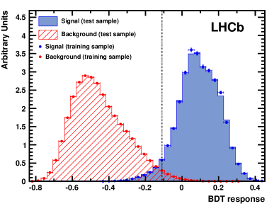
Figure 1: Distribution of the BDT algorithm response evaluated for background candidates from the data sidebands (red), and signal candidates from simulation (blue). The black dotted line indicates the chosen BDT response value.

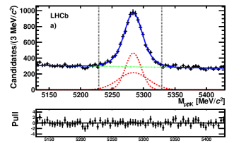
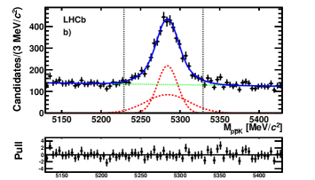
Figure 2: Invariant mass distribution of a) all selected $B^{+}\rightarrow p\bar{p}K^{+}$ candidates and b) candidates having $M_{p\bar{p}}<2.85\,{\rm{GeV/}}c^{2}$. The points with error bars are the data and the solid lines are the result of the fit. The dotted lines represent the two Gaussian functions (red) and the dashed line the linear function (green) used to parametrize the signal and the background, respectively. The vertical lines indicate the signal region. The two plots below the mass distributions show the pulls.

4 Signal yield determination

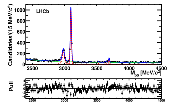
Figure 3: Invariant mass distribution of the $p\bar{p}$ system for $B^{+}\rightarrow p\bar{p}K^{+}$ candidates within the $B^{+}$ mass signal window, $|M(p\bar{p}K^{+})-M_{B^{+}}|<50\,{\rm{MeV/}}c^{2}$. The dotted lines represent the Gaussian and Voigtian functions (red) and the dashed line the smooth function (green) used to parametrize the signal and the background, respectively. The bottom plot shows the pulls.

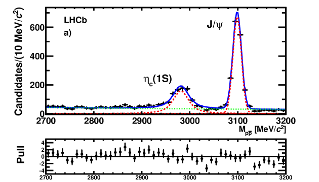
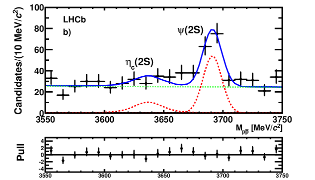
Figure 4: Invariant mass distribution of the $p\bar{p}$ system in the regions around a) the $\eta_{c}(1S)$ and $J/\psi$ and b) the $\eta_{c}(2S)$ and $\psi(2S)$ states. The dotted lines represent the Gaussian and the Voigtian functions (red) and the dashed line the smooth function (green) used to parametrize the signal and the background, respectively. The two plots below the mass distribution show the pulls.

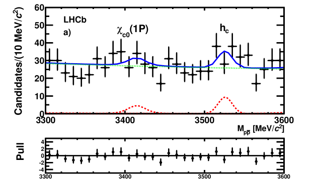
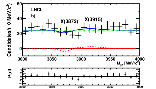
Figure 5: Invariant mass distribution of the $p\bar{p}$ system in the regions around a) the $\chi_{c0}(1P)$ and $h_{c}$ and b) the $X(3872)$ and $X(3915)$ states. The dotted lines represent the Gaussian and Voigitian functions (red) and the dashed line the smooth function (green) used to parametrize the signal and the background, respectively. The two plots below the mass distribution show the pulls.

The signal yield is determined from an unbinned extended maximum likelihood fit to the invariant mass of selected $B^{+}\rightarrow p\bar{p}K^{+}$ candidates, shown in Fig. 2a). The signal component is parametrized as the sum of two Gaussian functions with the same mean and different widths. The background component is parametrized as a linear function. The signal yield of the charmless component is determined by performing the same fit described above to the sample of $B^{+}\rightarrow p\bar{p}K^{+}$ candidates with $M_{p\bar{p}}<2.85\,{\rm{GeV/}}c^{2}$, shown in Fig. 2b). The $B^{+}$ mass and widths, evaluated with the invariant mass fits to all of the $B^{+}\rightarrow p\bar{p}K^{+}$ candidates, are compatible with the values obtained for the charmless component.

The signal yields for the charmonium contributions, $B^{+}\rightarrow(c\bar{c})K^{+}\rightarrow p\bar{p}K^{+}$, are determined by fitting the $p\bar{p}$ invariant mass distribution of $B^{+}\rightarrow p\bar{p}K^{+}$ candidates within the $B^{+}$ mass signal window, $|M_{p\bar{p}K^{+}}-M_{B^{+}}|<50\,{\rm{MeV/}}c^{2}$. Simulations show that no narrow structures are induced in the $p\bar{p}$ spectrum as kinematic reflections of possible $B^{+}\rightarrow p{\it\bar{\Lambda}}\rightarrow p\bar{p}K^{+}$ intermediate states.

An unbinned extended maximum likelihood fit to the $p\bar{p}$ invariant mass distribution, shown in Fig. 3, is performed over the mass range $2400-4500\,{\rm{MeV/}}c^{2}$. The signal components of the narrow resonances $J/\psi$, $\psi(2S)$, $h_{c}(1P)$, and $X(3872)$, whose natural widths are much smaller than the $p\bar{p}$ invariant mass resolution, are parametrized by Gaussian functions. The signal components for the $\eta_{c}(1S)$, $\chi_{c0}(1P)$, $\eta_{c}(2S)$, and $X(3915)$ are parametrized by Voigtian functions. Since the $p\bar{p}$ invariant mass resolution is approximately constant in the explored range, the resolution parameters for all resonances, except the $\psi(2S)$, are fixed to the $J/\psi$ value ($\sigma_{J/\psi}=8.9\pm 0.2\,{\rm{MeV/}}c^{2}$). The background shape is parametrized as $f(M)=e^{c_{1}M+c_{2}M^{2}}$ where $c_{1}$ and $c_{2}$ are fit parameters. The $J/\psi$ and $\psi(2S)$ resolution parameters, the mass values of the $\eta_{c}(1S)$, $J/\psi$, and $\psi(2S)$ states, and the $\eta_{c}(1S)$ natural width are left free in the fit. The masses and widths for the other signal components are fixed to the corresponding world averages [16]. The $p\bar{p}$ invariant mass resolution, determined by the fit to the $\psi(2S)$ is $\sigma_{\psi(2S)}=7.9\pm 1.7\,{\rm{MeV/}}c^{2}$.

The fit result is shown in Fig. 3. Figures 4 and 5 show the details of the fit result in the regions around the $\eta_{c}(1S)$ and $J/\psi$, $\eta_{c}(2S)$ and $\psi(2S)$, $\chi_{c0}(1P)$ and $h_{c}$, and $X(3872)$ and $X(3915)$ resonances. Any bias introduced by the inaccurate description of the tails of the $\eta_{c}(1S)$, $J/\psi$ and $\psi(2S)$ resonances is taken into account in the systematic uncertainty evaluation.

The contribution of $c\bar{c}\rightarrow p\bar{p}$ from processes other than $B^{+}\rightarrow p\bar{p}K^{+}$ decays, denoted as “non-signal”, is estimated from a fit to the $p\bar{p}$ mass in the $B^{+}$ mass sidebands $5130-5180$ and $5380-5430\,{\rm{MeV/}}c^{2}$. Except for the $J/\psi$ mode, no evidence of a non-signal contribution is found. The non-signal contribution to the $J/\psi$ signal yield in the $B^{+}$ mass window is $43\pm 11$ candidates and is subtracted from the number of $J/\psi$ signal candidates.

The signal yields, corrected for the non-signal contribution, are reported in Table 1. For the intermediate charmonium states $\eta_{c}(2S)$, $\chi_{c0}(1P)$, $h_{c}(1P)$, $X(3872)$ and $X(3915)$, there is no evidence of signal. The $95\%\,{\rm{CL}}$ upper limits on the number of candidates are shown in Table 1 and are determined from the likelihood profile integrating over the nuisance parameters. Since for the $X(3872)$ the fitted signal yield is negative, the upper limit has been calculated integrating the likelihood only in the physical region of a signal yield greater than zero.

Table 1: Signal yields for the different channels and corresponding 95%  CL upper limits for modes with less than 3$\sigma$ statistical significance. For the $J/\psi$ mode, the non-signal yield is subtracted. Uncertainties are statistical only.

$B^{+}$ decay mode	Signal yield		Upper limit (95%  CL)
$p\bar{p}K^{+}\;{\rm[total]}$	$6951\,$$\pm$	$\,176$
$p\bar{p}K^{+}\;[M_{p\bar{p}}<2.85\,{\rm{GeV/}}c^{2}]$	$3238\,$$\pm$	$\,122$
${J\mskip-3.0mu/\mskip-2.0mu\psi\mskip 2.0mu}K^{+}$	$1458\,$$\pm$	$\,42$
$\eta_{c}(1S)K^{+}$	$856\,$$\pm$	$\,46$
$\psi(2S)K^{+}$	$107\,$$\pm$	$\,16$
$\eta_{c}(2S)K^{+}$	$39\,$$\pm$	$\,15$	$<65.4$
$\chi_{c0}(1P)K^{+}$	$15\,$$\pm$	$\,13$	$<38.1$
$h_{c}(1P)K^{+}$	$21\,$$\pm$	$\,11$	$<40.2$
$X(3872)K^{+}$	$-9\,$$\pm$	$\,8$	$<10.3$
$X(3915)K^{+}$	$13\,$$\pm$	$\,17$	$<42.1$

5 Efficiency determination

The ratio of branching fractions is calculated using

$${\cal R}({\rm mode})=\frac{{\cal B}(B^{+}\rightarrow{\rm mode}\rightarrow p\bar{p}K^{+})}{{\cal B}(B^{+}\rightarrow J/\psi K^{+}\rightarrow p\bar{p}K^{+})}=\frac{N_{\rm mode}}{N_{{J\mskip-3.0mu/\mskip-2.0mu\psi\mskip 2.0mu}}}\times\frac{\epsilon_{{J\mskip-3.0mu/\mskip-2.0mu\psi\mskip 2.0mu}}}{\epsilon_{\rm mode}},$$ (2)

where $N_{\rm mode}$ and $N_{{J\mskip-3.0mu/\mskip-2.0mu\psi\mskip 2.0mu}}$ are the signal yields for the given mode and the reference mode, $B^{+}\rightarrow{J\mskip-3.0mu/\mskip-2.0mu\psi\mskip 2.0mu}K^{+}\rightarrow p\bar{p}K^{+}$, and $\epsilon_{\rm mode}/\epsilon_{{J\mskip-3.0mu/\mskip-2.0mu\psi\mskip 2.0mu}}$ is the corresponding ratio of efficiencies. The efficiency is the product of the reconstruction, trigger, and selection efficiencies, and is estimated using simulated data samples.

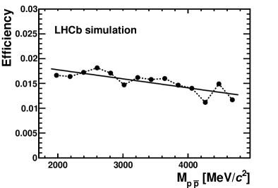
Figure 6: Efficiency as a function of $M_{p\bar{p}}$ for $B^{+}\rightarrow p\bar{p}K^{+}$ decays. The solid line represents the linear fit to the efficiency distribution; the dashed line is the point-by-point interpolation used to estimate the systematic uncertainty.

Since the track multiplicity distribution for simulated events differs from that observed in data, simulated candidates are assigned a weight so that the weighted distribution reproduces the observed multiplicity distribution. The distributions of $\Delta$ln${\mathcal{L}}_{K\pi}$ and $\Delta$ln${\mathcal{L}}_{p\pi}$ for kaons and protons in data are obtained in bins of momentum, pseudorapidity and number of tracks from control samples of $D^{*+}\rightarrow D^{0}(\rightarrow K^{-}\pi^{+})\pi^{+}$ decays for kaons and ${\it\mathchar 28931\relax}\rightarrow p\pi^{-}$ decays for protons, which are then used on a track-by-track basis to correct the simulation. The efficiency as a function of $M_{p\bar{p}}$ is shown in Fig. 6. A linear fit to the efficiency distribution is performed and the efficiency ratios are determined based on the fit result.

Table 2: Relative systematic uncertainties (in $\%$) on the relative branching fractions from different sources. The total systematic uncertainty is determined by adding the individual contributions in quadrature.

Source	${\cal R}({\rm total})$	${\cal R}(M_{p\bar{p}}<2.85\,{\rm{GeV/}}c^{2})$	${\cal R}(\eta_{c}(1S))$	${\cal R}(\psi(2S))$
Efficiency ratio	0.21	0.5	3.3	4.8
$B^{+}$ mass fit range	0.16	0.5	$-$	$-$
Sig. and Bkg. shape	2.5	3.6	1.8	6.5
$B^{+}$ mass window	0.6	0.6	0.9	3.8
Non-signal component	$-$	$-$	0.4	5.1
Signal tail param.	1.0	1.0	1.2	4.3
Total	2.8	3.8	4.1	11.3

Source	${\cal R}(\eta_{c}(2S))$	${\cal R}(\chi_{c0}(1P))$	${\cal R}(h_{c}(1P))$	${\cal R}(X(3872))$	${\cal R}(X(3915))$
Efficiency ratio	4.4	2.5	3.4	6.5	7.0
$B^{+}$ mass fit range	$-$	$-$	$-$	$-$
Sig. and Bkg. shape	3.9	3.3	14.3	5.6	10.1
$B^{+}$ mass window	11.3	23.6	23.6	17.5	7.5
Non-signal component	$-$	$-$	$-$	$-$	$-$
Signal tail param.	1.0	1.0	1.0	1.0	1.0
Total	12.8	24.0	27.8	19.5	15.5

6 Systematic uncertainties

The measurements of the relative branching fractions depend on the ratios of signal yields and efficiencies with respect to the reference mode. Since the final state is the same in all cases, most of the systematic uncertainties cancel. The systematic uncertainty on the efficiency ratio, in each region of $p\bar{p}$ invariant mass, is determined from the difference between the efficiency ratios calculated using the solid fitted line and the dashed point-by-point interpolation shown in Fig. 6. The uncertainty associated with the evaluation of the $B^{+}$ signal yield has been determined by varying the fit range by $\pm 30\,{\rm{MeV/}}c^{2}$, using a single Gaussian instead of a double Gaussian function to model the signal PDF, and using an exponential function to model the background. For each charmonium resonance the systematic uncertainty on the signal yield has been investigated by varying the $B$ mass signal window by $\pm 10\,{\rm{MeV/}}c^{2}$, the signal and background shape parametrization and the subtraction of the $c\bar{c}$ contribution from the continuum. The systematic uncertainty associated with the parametrization of the signal tails of the $J/\psi$, $\eta_{c}(1S)$ and $\psi(2S)$ resonances is taken into account by taking the difference between the number of candidates in the observed distribution and the number of candidates calculated from the integral of the fit function in the range $-6\sigma$ to $-2.5\sigma$. The systematic uncertainty associated with the selection procedure is estimated by changing the value of the BDT selection to $-0.03$, which retains $85\%$ of the signal with a $30\%$ background, and is found to be negligible. The contributions to the systematic uncertainties from the different sources are listed in Table 2. The total systematic uncertainty is determined by adding the individual contributions in quadrature.

7 Results

The results are summarized in Table 3 and the values of the product of branching fractions derived from our measurement using the world average values ${\cal B}(B^{+}\rightarrow J/\psi K^{+})=(1.013\pm 0.034)\times 10^{-3}$ and ${\cal B}(J/\psi\rightarrow p\bar{p})=(2.17\pm 0.07)\times 10^{-3}$ [16] are listed in Table 4.

Table 3: Signal yields, efficiency ratios, ratios of branching fractions and corresponding upper limits.

$B^{+}\rightarrow({\rm mode})$	Yield			$\epsilon_{\rm mode}/\epsilon_{J\mskip-3.0mu/\mskip-2.0mu\psi\mskip 2.0mu}$	${\cal R}({\rm mode})$			Upper Limit
$\rightarrow p\bar{p}K^{+}$	$\pm$ stat $\pm$ syst			$\pm$ syst	$\pm$ stat $\pm$ syst			$95\%$ CL
${J\mskip-3.0mu/\mskip-2.0mu\psi\mskip 2.0mu}K^{+}$	$1458\,$$\pm$	$\,42\,$$\pm$	$\,24$	$-$	1			$-$
total	$6951\,$$\pm$	$\,176\,$$\pm$	$\,171$	$0.970\pm 0.002$	$4.91\,$$\pm$	$\,0.19\,$$\pm$	$\,0.14$	$-$
${M_{p\bar{p}}<2.85\,{\rm{GeV/}}c^{2}}$	$3238\,$$\pm$	$\,122\,$$\pm$	$\,121$	$1.097\pm 0.006$	$2.02\,$$\pm$	$\,0.10\,$$\pm$	$\,0.08$	$-$
$\eta_{c}(1S)K^{+}$	$856\,$$\pm$	$\,46\,$$\pm$	$\,19$	$1.016\pm 0.034$	$0.578\,$$\pm$	$\,0.035\,$$\pm$	$\,0.026$	$-$
$\psi(2S)K^{+}$	$107\,$$\pm$	$\,16$$\pm$	$\,13$	$0.921\pm 0.044$	$0.080\,$$\pm$	$\,0.012\,$$\pm$	$\,0.009$	$-$
$\eta_{c}(2S)K^{+}$	$39\,$$\pm$	$\,15\,$$\pm$	$\,5$	$0.927\pm 0.041$	$0.029\,$$\pm$	$\,0.011\,$$\pm$	$\,0.004$	$<0.048$
$\chi_{c0}(1P)K^{+}$	$15\,$$\pm$	$\,13\,$$\pm$	$\,4$	$0.957\pm 0.024$	$0.011\,$$\pm$	$\,0.009\,$$\pm$	$\,0.003$	$<0.028$
$h_{c}(1P)K^{+}$	$21\,$$\pm$	$\,11\,$$\pm$	$\,5$	$0.943\pm 0.032$	$0.015\,$$\pm$	$\,0.008\,$$\pm$	$\,0.004$	$<0.029$
$X(3872)K^{+}$	$-9\,$$\pm$	$\,8\,$$\pm$	$\,2$	$0.896\pm 0.058$	$-0.007\,$$\pm$	$\,0.006\,$$\pm$	$\,0.002$	$<0.008$
$X(3915)K^{+}$	$13\,$$\pm$	$\,17\,$$\pm$	$\,5$	$0.890\pm 0.062$	$0.010\,$$\pm$	$\,0.013\,$$\pm$	$\,0.002$	$<0.032$

Table 4: Branching fractions for $B^{+}\rightarrow({\rm mode})\rightarrow p\bar{p}K^{+}$ derived using the world average value of the ${\cal B}(B^{+}\rightarrow{J\mskip-3.0mu/\mskip-2.0mu\psi\mskip 2.0mu}K^{+})$ and ${\cal B}({J\mskip-3.0mu/\mskip-2.0mu\psi\mskip 2.0mu}\rightarrow p\bar{p})$ branching fractions [16]. For the charmonium modes we compare our values to the product of the indipendently measured branching fractions. The first uncertainties are statistical, the second systematic in the present measurement, and the third systematic from the uncertainty on the $J/\psi$ branching fraction.

$B^{+}$	${\cal B}(B^{+}\rightarrow({\rm mode})\rightarrow p\bar{p}K^{+})$				UL $(95\%$ CL)	Previous measurements
decay mode	($\times 10^{6}$)				($\times 10^{6}$)	($\times 10^{6}$) [4, 5]
total	$10.81\,$$\pm$	$\,0.42\,$$\pm$	$\,0.30\,$$\pm$	$\,0.49$		$10.76^{+0.36}_{-0.33}\pm 0.70$
${M_{p\bar{p}}<2.85\,{\rm{GeV/}}c^{2}}$	$4.46\,$$\pm$	$\,0.21\,$$\pm$	$\,0.18\,$$\pm$	$\,0.20$		$5.12\pm 0.31$
$\eta_{c}(1S)K^{+}$	$1.27\,$$\pm$	$\,0.08\,$$\pm$	$\,0.05\,$$\pm$	$\,0.06\,$		$1.54\pm 0.16$
$\psi(2S)K^{+}$	$0.175\,$$\pm$	$\,0.027\,$$\pm$	$\,0.020\,$$\pm$	$\,0.008$		$0.176\pm 0.012$
$\eta_{c}(2S)K^{+}$	$0.063\,$$\pm$	$\,0.025\,$$\pm$	$\,0.009\,$$\pm$	$\,0.003$	$<0.106$
$\chi_{c0}(1P)K^{+}$	$0.024\,$$\pm$	$\,0.021\,$$\pm$	$\,0.006\,$$\pm$	$\,0.001$	$<0.062$	$0.030\pm 0.004$
$h_{c}(1P)K^{+}$	$0.034\,$$\pm$	$\,0.018\,$$\pm$	$\,0.008\,$$\pm$	$\,0.002$	$<0.064$
$X(3872)K^{+}$	$-0.015\,$$\pm$	$\,0.013\,$$\pm$	$\,0.003\,$$\pm$	$\,0.001$	$<0.017$
$X(3915)K^{+}$	$0.022\,$$\pm$	$\,0.029\,$$\pm$	$\,0.004\,$$\pm$	$\,0.001$	$<0.071$

The branching fractions obtained are compatible with the world average values [16]. The upper limit on ${\mathcal{B}}(B^{+}\rightarrow\chi_{c0}(1P)K^{+}\rightarrow p\bar{p}K^{+})$ is compatible with the world average ${\mathcal{B}}(B^{+}\rightarrow\chi_{c0}(1P)K^{+})\times{\mathcal{B}}(\chi_{c0}(1P)\rightarrow p\bar{p})=(0.030\pm 0.004)\times 10^{-6}$ [16]. We combine our upper limit for $X(3872)$ with the known value for ${\mathcal{B}}(B^{+}\rightarrow X(3872)K^{+})\times{\mathcal{B}}(X(3872)\rightarrow J/\psi\pi^{+}\pi^{-})=(8.6\pm 0.8)\times 10^{-6}$ [16] to obtain the limit

$$\frac{{\mathcal{B}}(X(3872)\rightarrow p\bar{p})}{{\mathcal{B}}(X(3872)\rightarrow J/\psi\pi^{+}\pi^{-})}<2.0\times 10^{-3}.$$

This limit challenges some of the predictions for the molecular interpretations of the $X(3872)$ state and is approaching the range of predictions for a conventional $\chi_{c1}(2P)$ state [17, 18]. Using our result and the $\eta_{c}(2S)$ branching fraction ${\mathcal{B}}(B^{+}\rightarrow\eta_{c}(2S)K^{+})\times{\mathcal{B}}(\eta_{c}(2S)\rightarrow K\bar{K}\pi)=(3.4\,^{+2.3}_{-1.6})\times 10^{-6}$ [16], a limit of

$$\frac{{\mathcal{B}}(\eta_{c}(2S)\rightarrow p\bar{p})}{{\mathcal{B}}(\eta_{c}(2S)\rightarrow K\bar{K}\pi)}<3.1\times 10^{-2}$$

is obtained.

8 Summary

Based on a sample of $6951\pm 176$ $B^{+}\rightarrow p\bar{p}K^{+}$ decays reconstructed in a data sample, corresponding to an integrated luminosity of $1.0\,{\rm{fb^{-1}}}$, collected with the LHCb detector, the following relative branching fractions are measured

$$\frac{{\mathcal{B}}(B^{+}\rightarrow p\bar{p}K^{+})_{\rm total}}{{\mathcal{B}}(B^{+}\rightarrow J/\psi K^{+}\rightarrow p\bar{p}K^{+})}= \,4.91\pm 0.19\,{(\rm stat)}\pm 0.14\,{(\rm syst)},$$

$$\frac{{\mathcal{B}}(B^{+}\rightarrow p\bar{p}K^{+})_{M_{p\bar{p}}<2.85\,{\rm{GeV/}}c^{2}}}{{\mathcal{B}}(B^{+}\rightarrow J/\psi K^{+}\rightarrow p\bar{p}K^{+})}= \,2.02\pm 0.10\,{(\rm stat)}\pm 0.08\,{(\rm syst)},$$

$$\frac{{\mathcal{B}}(B^{+}\rightarrow\eta_{c}(1S)K^{+}\rightarrow p\bar{p}K^{+})}{{\mathcal{B}}(B^{+}\rightarrow J/\psi K^{+}\rightarrow p\bar{p}K^{+})}= \,0.578\pm 0.035\,{(\rm stat)}\pm 0.025\,{(\rm syst)},$$

$$\frac{{\mathcal{B}}(B^{+}\rightarrow\psi(2S)K^{+}\rightarrow p\bar{p}K^{+})}{{\mathcal{B}}(B^{+}\rightarrow J/\psi K^{+}\rightarrow p\bar{p}K^{+})}= \,0.080\pm 0.012\,{(\rm stat)}\pm 0.009\,{(\rm syst)}.$$

An upper limit on the ratio $\frac{{\mathcal{B}}(B^{+}\rightarrow X(3872)K^{+}\rightarrow p\bar{p}K^{+})}{{\mathcal{B}}(B^{+}\rightarrow J/\psi K^{+}\rightarrow p\bar{p}K^{+})}<0.017$ is obtained, from which a limit of

$$\frac{{\mathcal{B}}(X(3872)\rightarrow p\bar{p})}{{\mathcal{B}}(X(3872)\rightarrow J/\psi\pi^{+}\pi^{-})}<2.0\times 10^{-3}$$

is derived.

References

- [1] N. Brambilla et al., Heavy quarkonium: progress, puzzles, and opportunities, Eur. Phys. J. C71 (2011) 1534, arXiv:1010.5827
- [2] LHCb collaboration, R. Aaij et al., Determination of the X(3872) meson quantum numbers, arXiv:1302.6269
- [3] J. S. Lange et al., Prospects for X(3872) detection at Panda, AIP Conf. Proc. 1374 (2011) 549, arXiv:1010.2350
- [4] BaBar collaboration, B. Aubert et al., Measurement of the branching fraction and study of the decay dynamics, Phys. Rev. D72 (2005) 051101, arXiv:hep-ex/0507012
- [5] Belle collaboration, J. Wei et al., Study of and , Phys. Lett. B659 (2008) 80, arXiv:0706.4167
- [6] LHCb collaboration, J. Alves, A. Augusto et al., The LHCb detector at the LHC, JINST 3 (2008) S08005
- [7] R. Aaij et al., The LHCb trigger and its performance, arXiv:1211.3055, submitted to JINST
- [8] T. Sjöstrand, S. Mrenna, and P. Skands, PYTHIA 6.4 Physics and manual, JHEP 05 (2006) 026, arXiv:hep-ph/0603175
- [9] I. Belyaev et al., Handling of the generation of primary events in Gauss, the LHCb simulation framework, Nuclear Science Symposium Conference Record (NSS/MIC) IEEE (2010) 1155
- [10] D. J. Lange, The EvtGen particle decay simulation package, Nucl. Instrum. Meth. A462 (2001) 152
- [11] P. Golonka and Z. Was, PHOTOS Monte Carlo: a precision tool for QED corrections in and decays, Eur. Phys. J. C45 (2006) 97, arXiv:hep-ph/0506026
- [12] GEANT4 collaboration, J. Allison et al., Geant4 developments and applications, IEEE Trans. Nucl. Sci. 53 (2006) 270
- [13] GEANT4 collaboration, S. Agostinelli et al., GEANT4: a simulation toolkit, Nucl. Instrum. Meth. A506 (2003) 250
- [14] M. Clemencic et al., The LHCb simulation application, Gauss: design, evolution and experience, J. of Phys: Conf. Ser. 331 (2011) 032023
- [15] L. Breiman, J. H. Friedman, R. A. Olshen, and C. J. Stone, Classification and regression trees. Wadsworth international group, Belmont, California, USA, 1984
- [16] Particle Data Group, J. Beringer et al., Review of Particle Physics (RPP), Phys. Rev. D86 (2012) 010001
- [17] G. Chen and J. Ma, Production of at PANDA, Phys. Rev. D77 (2008) 097501, arXiv:0802.2982
- [18] E. Braaten, An estimate of the partial width for into , Phys. Rev. D77 (2008) 034019, arXiv:0711.1854