Complex hyperbolic geometry of the figure eight knot

Abstract.

We show that the figure eight knot complement admits a uniformizable spherical CR structure, i.e. it occurs as the manifold at infinity of a complex hyperbolic orbifold. The uniformization is unique provided we require the peripheral subgroups to have unipotent holonomy.

1. Introduction

The general framework of this paper is the study of the interplay between topological properties of $3$-manifolds and the existence of geometric structures. The model result along these lines is of course Thurston’s geometrization conjecture, recently proved by Perelman, that contains a topological characterization of manifolds that admit a geometry modeled on real hyperbolic space ${{\bf H}^{3}_{\mathbb{R}}}$. Beyond an existence result (under the appropriate topological assumptions), the hyperbolic structures can in fact be constructed fairly explicitly, as one can easily gather by reading Thurston’s notes [20], where a couple of explicit examples are worked out.

The idea is to triangulate the manifold, and to try and realize each tetrahedron geometrically in ${{\bf H}^{3}_{\mathbb{R}}}$. The gluing pattern of the tetrahedra imposes compatibility conditions on the parameters of the tetrahedra, and it turns out that solving these compatibility equations is very often equivalent to finding the hyperbolic structure. The piece of software called SnapPea, originally developed by Jeff Weeks (and under constant development to this day), provides an extremely efficient way to construct explicit hyperbolic structures on 3-manifolds.

In this paper, we are interested in using the $3$-sphere $S^{3}$ as the model geometry, with the natural structure coming from describing it as the boundary of the unit ball $\mathbb{B}^{2}\subset\mathbb{C}^{2}$. Any real hypersurface in $\mathbb{C}^{2}$ inherits what is called a CR structure (the largest subbundle in the tangent bundle that is invariant under the complex structure), and such a structure is called spherical when it is locally equivalent to the CR structure of $S^{3}$. Local equivalence to $S^{3}$ in the sense of CR structures translates into the existence of an atlas of charts with values in $S^{3}$, and with transition maps given by restrictions of biholomorphisms of $\mathbb{B}^{2}$, i.e. elements of $\mathbf{PU}(2,1)$, see [3].

In other words, a spherical CR structure is a $(G,X)$-structure with $G=\mathbf{PU}(2,1)$, $X=S^{3}$. The central motivating question is to give a characterization of $3$-manifolds that admit a spherical CR structure; the only negative result in that direction is given by Goldman [9], who classifies $T^{2}$-bundles over $S^{1}$ that admit spherical CR structures (only those with Nil geometry admit spherical CR structures).

An important class of spherical CR structures is the class of uniformizable spherical CR structures. These are obtained from discrete subgroups $\Gamma\subset\mathbf{PU}(2,1)$ by taking the quotient of the domain of discontinuity $\Omega$ by the action of $\Gamma$ (we assume that $\Omega$ is non-empty, and that $\Gamma$ has no fixed point on $\Omega$, so that the quotient is indeed a manifold). The structure induced from the standard CR structure on $S^{3}$ on the quotient $M=\Gamma\setminus\Omega$ is then called a uniformizable spherical CR structure on $M$.

When a manifold $M$ can be written as above for some group $\Gamma$, we will also simply say that $M$ admits a spherical CR uniformization. Our terminology differs slightly from the recent literature on the subject, where uniformizable structures are sometimes referred to as complete structures (see [19] for instance).

Of course one wonders which manifolds admit spherical CR uniformizations, and how restrictive it is to require the existence of a spherical CR uniformization as opposed to a general spherical CR structure. For instance, when $\Gamma$ is a finite group acting without fixed points on $S^{3}$, $\Omega=S^{3}$ and $\Gamma\setminus S^{3}$ gives the simplest class of examples (including lens spaces).

The class of circle bundles over surfaces has been widely explored, and many such bundles are known to admit uniformizable spherical CR structures, see the introduction of [19] and the references given there. It is also known that well-chosen deformations of triangle groups produce spherical CR structures on more complicated $3$-manifolds, including real hyperbolic ones. Indeed, Schwartz showed in [17] that the Whitehead link complement admits a uniformizable spherical CR structure, and in [18] he found an example of a closed hyperbolic manifold that arises as the boundary of a complex hyperbolic surface. Once again, we refer the reader to the [19] for a detailed overview of the history of this problem.

All these examples are obtained by analyzing special classes of discrete groups, and checking the topological type of their manifold at infinity. In the opposite direction, given a $3$-manifold $M$, one would like a method to construct (and possibly classify) all structures on $M$, in the spirit of the constructive version of hyperbolization alluded to earlier in this introduction.

A step in that direction was proposed by the second author in [5], based on triangulations and adapting the compatibility equations to the spherical CR setting. Here, a basic difficulty is that there is no canonical way to associate a tetrahedron to a given quadruple of points in $S^{3}$. Even the $1$-skeleton is elusive, since arcs of $\mathbb{C}$-circles (or $\mathbb{R}$-circles) between two points are not unique (see section 2.1 for definitions).

A natural way over this difficulty is to formulate compatibility conditions that translate the possibility of geometric realization in $S^{3}$ only on the level of the vertices of the tetrahedra. Indeed, ordered generic quadruples of points are parametrized up to isometry by appropriate cross ratios, and one can easily write down the corresponding compatibility conditions explicitly [5].

Given a solution of these compatibility equations, one always gets a representation $\rho:\pi_{1}(M)\rightarrow\mathbf{PU}(2,1)$, but it is not clear whether or not the quadruples of points can be extended to actual tetrahedra in a $\rho$-equivariant way (in other words, it is not clear whether or not $\rho$ is the holonomy of an actual structure).

There are many solutions to the compatibility equations, so we will impose a restriction on the representation $\rho$, namely that $\rho(\pi_{1}(T))$ be unipotent for each torus boundary component $T$ of $M$. This is a very stringent condition, but it is natural since it holds for complete hyperbolic metrics of finite volume.

For the remainder of the paper, we will concentrate on a specific $3$-manifold, namely the figure eight knot complement, and give encouraging signs for the philosophy outlined in the preceding paragraphs. Indeed, for that specific example, we will check that the solutions to the compatibility equations give a spherical CR uniformization of the figure eight knot, which is unique provided we require the boundary holonomy to consist only of unipotent isometries (in fact we get one structure for each orientation on $M$, see section 9).

We work with the figure eight knot complement partly because it played an important motivational role in the eighties for the development of real hyperbolic geometry. It is well known that this non-compact manifold $M$ admits a unique complete hyperbolic metric, with one torus end (which one may think of as a tubular neighborhood of the figure eight knot). This is originally due to Riley, see [15].

It is also well known that $M$ can be triangulated with just two tetrahedra (this triangulation is far from simplicial, but this is irrelevant in the present context). The picture in Figure 1 can be found for instance in the first few pages of Thurston’s notes [20].

Figure 1. The figure eight knot complement can be obtained by gluing two tetrahedra (a face on the left and a face on the right are identified if the corresponding pattern of arrows agree), and removing the vertices.

The above decomposition can be realized geometrically in ${{\bf H}^{3}_{\mathbb{R}}}$ (and the corresponding geometric tetrahedra are regular tetrahedra, so the volume of this metric is $6\textcyr{L}(\pi/3)\approx 2.029$).

For the specific triangulation of the figure eight knot complement depicted in Figure 1, all the solutions of the compatibility equations were given in [5], without detailed justification of the fact that the list of solutions is exhaustive. The explanation of exhaustivity now appears in various places in the literature (see [2] and [8], and also [6] for more general 3-manifolds). It turns out there are only three solutions to the compatibility equations (up to complex conjugation of the cross ratios parametrizing the tetrahedra), yielding three representations $\rho_{1}$, $\rho_{2}$ and $\rho_{3}:\pi_{1}(M)\rightarrow\mathbf{PU}(2,1)$ (in fact six representations, if we include their complex conjugates). Throughout the paper, we will denote by $\Gamma_{k}$ the image of $\rho_{k}$.

It was shown in [5] that $\rho_{1}$ is the holonomy of a branched spherical CR structure (the corresponding developing map is a local diffeomorphism away from a curve), and that the limit set of $\Gamma_{1}$ is equal to $\partial_{\infty}{{\bf H}^{2}_{\mathbb{C}}}$, hence the quotient $\Gamma_{1}\setminus{{\bf H}^{2}_{\mathbb{C}}}$ has empty manifold at infinity. In particular, no spherical CR structure with holonomy $\rho_{1}$ can ever be uniformizable. In [7], a branched structure with holonomy $\rho_{2}$ is constructed, which is again not a uniformization.

The main goal of this paper is to show that $\rho_{2}$ and $\rho_{3}$ are holonomy representations of unbranched uniformizable spherical CR structures on the figure eight knot complement. These two representations are not conjugate in $\mathbf{PU}(2,1)$, but it turns out that the images $\Gamma_{2}$ and $\Gamma_{3}$ are in fact conjugate.

The precise relationship between the two structures corresponding to $\rho_{2}$ and $\rho_{3}$ will be explained by the existence of an orientation-reversing diffeomorphism of the figure eight knot complement (which follows from the fact that this knot is amphichiral). Indeed, given a diffeomorphism $\alpha:M\rightarrow\Gamma_{2}\setminus\Omega_{2}$, and an an orientation-reversing diffeomorphism $\varphi:M\rightarrow M$, $\alpha\circ\varphi$ defines a spherical CR structure on $M$ with the opposite orientation. We will see that $\rho_{2}$ and $\rho_{3}$ are obtained from each other by this orientation switch (see section 8). For that reason, we will work only with $\rho_{2}$ for most of the paper.

We denote by $\Gamma$ the group $\Gamma_{2}$. Our main result is the following.

Theorem 1.1.

The domain of discontinuity $\Omega$ of $\Gamma$ is non empty. The action of $\Gamma$ has no fixed points in $\Omega$, and the quotient $\Gamma\setminus\Omega$ is homeomorphic to the figure eight knot complement.

In other words, the figure eight knot admits a spherical CR uniformization, with uniformization given by $\Gamma$. The uniformization is not quite unique, but we will show that it is unique provided we require the boundary holonomy to be unipotent (see Proposition 3.1).

The fact that the ideal boundary of $\Gamma\setminus{{\bf H}^{2}_{\mathbb{C}}}$ is indeed a manifold, and not just an orbifold, follows from the fact that every elliptic element in $\Gamma$ has an isolated fixed point in ${{\bf H}^{2}_{\mathbb{C}}}$ (we will be able to list all conjugacy classes of elliptic elements, by using the cycles of the fundamental domain, see Proposition 5.6).

The result of Theorem 1.1 is stated in terms of the domain of discontinuity which is contained in $\partial_{\infty}{{\bf H}^{2}_{\mathbb{C}}}$, so one may expect the arguments to use properties of $S^{3}\subset\mathbb{C}^{2}$ or Heisenberg geometry (see section 2.1). In fact the bulk of the proof is about the relevant complex hyperbolic orbifold $\Gamma\setminus{{\bf H}^{2}_{\mathbb{C}}}$, and for most of the paper, we will use geometric properties of ${{\bf H}^{2}_{\mathbb{C}}}$.

The basis of our study of the manifold at infinity will be the Dirichlet domain for $\Gamma$ centered at a strategic point, namely the isolated fixed point of $G_{2}=\rho_{2}(g_{2})$ (see section 3 for notation). This domain is not a fundamental domain for the action of $\Gamma$ (the center is stabilized by a cyclic group of order $4$), but it is convenient because it has very few faces (in fact all its faces are isometric to each other). In particular, we get an explicit presentation for $\Gamma$, given by

(1) $$\langle\ G_{1},G_{2}\ |\ G_{2}^{4},\ (G_{1}G_{2})^{3},\ (G_{2}G_{1}G_{2})^{3}\ \rangle$$

Note that $\rho_{2}$ is of course not a faithful representation of the figure eight knot group. In fact from the above presentation, it is easy to determine normal generators for the kernel of $\rho_{2}$, see Proposition 5.7.

Acknowledgements: This work was supported in part by the ANR through the project Structure Géométriques et Triangulations. The authors wish to thank Christine Lescop, Antonin Guilloux, Julien Marché, Jean-Baptiste Meilhan, Jieyan Wang, Pierre Will and Maxime Wolff for useful discussions related to the paper. They are also very grateful to the referees for many useful remarks that helped improve the exposition.

2. Basics of complex hyperbolic geometry

2.1. Complex hyperbolic geometry

In this section we briefly review basic facts and notation about the complex hyperbolic plane. For more information, see [10].

We denote by $\mathbb{C}^{2,1}$ the three-dimensional complex vector space $\mathbb{C}^{3}$ equipped with the Hermitian form

$$\langle Z,W\rangle=Z_{1}\overline{W}_{3}+Z_{2}\overline{W}_{2}+Z_{3}\overline{W}_{1}.$$

The subgroup of $GL(3,\mathbb{C})$ preserving the Hermitian form $\langle\cdot,\cdot\rangle$ is denoted by $\mathbf{U}(2,1)$, and its action preserves each of the following three sets:

$$V_{+}=\{Z\in\mathbb{C}^{2,1}:\langle Z,Z\rangle>0\},$$

$$V_{0}=\{Z\in\mathbb{C}^{2,1}-\{0\}:\langle Z,Z\rangle=0\},$$

$$V_{-}=\{Z\in\mathbb{C}^{2,1}:\langle Z,Z\rangle<0\}.$$

Let $P:\mathbb{C}^{2,1}-\{0\}\rightarrow{{\bf P}^{2}_{\mathbb{C}}}$ be the canonical projection onto complex projective space, and let $\mathbf{PU}(2,1)$ denote the quotient of $\mathbf{U}(2,1)$ by scalar matrices, which acts effectively on ${{\bf P}^{2}_{\mathbb{C}}}$. Note that the action of $\mathbf{PU}(2,1)$ is transitive on $P(V_{\pm})$ and on $P(V_{0})$. Up to scalar multiples, there is a unique Riemannian metric on $P(V_{-})$ invariant under the action of $\mathbf{PU}(2,1)$, which turns it into a Hermitian symmetric space often denoted by ${{\bf H}^{2}_{\mathbb{C}}}$, and called the complex hyperbolic plane. In the present paper, we will not need a specific normalization of the metric. We mention for completeness that any invariant metric is Kähler, with holomorphic sectional curvature a negative constant (the real sectional curvatures are $1/4$-pinched).

The full isometry group of ${{\bf H}^{2}_{\mathbb{C}}}$ is given by

$$\widehat{\mathbf{PU}(2,1)}=\langle\mathbf{PU}(2,1),{\mathbf{\iota}}\rangle,$$

where ${\mathbf{\iota}}$ is given by complex conjugation $Z\mapsto\overline{Z}$ on the level of homogeneous coordinates.

Still denoting $(Z_{1},Z_{2},Z_{3})$ the coordinates of $\mathbb{C}^{3}$, one easily checks that $V_{-}$ can contain no vector with $Z_{3}=0$, hence we can describe its image in ${{\bf P}^{2}_{\mathbb{C}}}$ in terms of non-homogeneous coordinates $w_{1}=Z_{1}/Z_{3}$, $w_{2}=Z_{2}/Z_{3}$, where $P(V_{-})$ corresponds to the Siegel half space

$$|w_{1}|^{2}+2\ {\rm Re}\ w_{2}<0.$$

The ideal boundary of complex hyperbolic space is defined as $\partial_{\infty}{{\bf H}^{2}_{\mathbb{C}}}=P(V_{0})$. It is described almost entirely in the affine chart $Z_{3}\neq 0$ used to define the Siegel half space, only $(1,0,0)$ is sent off to infinity. We denote by $p_{\infty}$ the corresponding point in $\partial_{\infty}{{\bf H}^{2}_{\mathbb{C}}}$.

The unipotent stabilizer of $(1,0,0)$ acts simply transitively on $\partial_{\infty}{{\bf H}^{2}_{\mathbb{C}}}\setminus\{p_{\infty}\}$, which allows us to identify $\partial_{\infty}{{\bf H}^{2}_{\mathbb{C}}}$ with the one-point compactification of the Heisenberg group $\mathfrak{N}$.

Here recall that $\mathfrak{N}$ is defined as $\mathbb{C}\times\mathbb{R}$ equipped with the following group law

$$(z,t)\cdot(z^{\prime},t^{\prime})=(z+z^{\prime},t+t^{\prime}+2\Im(z\overline{z}^{\prime})).$$

Any point $p=(z,t)\in\mathfrak{N}$ has the following lift to $\mathbb{C}^{2,1}$:

$$\tilde{p}=\left[\begin{array}[]{c}(-|z|^{2}+it)/2\\ z\\ 1\end{array}\right]$$

while $p_{\infty}$ lifts to $(1,0,0)$.

It is a standard fact that the above form can be diagonalized, say by using the change of homogeneous coordinates given by $U_{2}=Z_{2}$, $U_{1}=(Z_{1}+Z_{3})/\sqrt{2}$, $U_{3}=(Z_{1}-Z_{3})/\sqrt{2}$. With these coordinates, the Hermitian form reads

$$\langle U,V\rangle=U_{1}\overline{V}_{1}+U_{2}\overline{V}_{2}-U_{3}\overline{V}_{3},$$

and in the affine chart $U_{3}\neq 0$, with coordinates $u_{1}=U_{1}/U_{3}$, $u_{2}=U_{2}/U_{3}$, ${{\bf H}^{2}_{\mathbb{C}}}$ corresponds to the unit ball $\mathbb{B}^{2}\subset\mathbb{C}^{2}$, given by

$$|u_{1}|^{2}+|u_{2}|^{2}<1.$$

In this model the ideal boundary is simply given by the unit sphere $S^{3}\subset\mathbb{C}^{2}$. This gives $\partial_{\infty}{{\bf H}^{2}_{\mathbb{C}}}$ a natural CR-structure (see the introduction and the references given there).

We will use the classification of isometries of negatively curved spaces into elliptic, parabolic and loxodromic elements, as well as a slight algebraic refinement; an elliptic isometry is called regular elliptic if its matrix representatives have distinct eigenvalues.

Non-regular elliptic elements in $\mathbf{PU}(2,1)$ fix a projective line in ${{\bf P}^{2}_{\mathbb{C}}}$, hence they come into two classes, depending on the position of that line with respect to ${{\bf H}^{2}_{\mathbb{C}}}$. If the projective line intersects ${{\bf H}^{2}_{\mathbb{C}}}$, the corresponding isometry is called a complex reflection in a line; if it does not intersect $\partial_{\infty}{{\bf H}^{2}_{\mathbb{C}}}$, then the isometry is called a complex reflection in a point. Complex reflections in points do not have any fixed points in the ideal boundary.

The only parabolic elements we will use in this paper will be unipotent (i.e. some matrix representative in $\mathbf{U}(2,1)$ has $1$ as its only eigenvalue).

Finally, we mention the classification of totally geodesic submanifolds in ${{\bf H}^{2}_{\mathbb{C}}}$. There are two kinds of totally geodesic submanifolds of real dimension two, complex geodesics (which can be thought of copies of ${{\bf H}^{1}_{\mathbb{C}}}$), and totally real totally geodesic planes (copies of ${{\bf H}^{2}_{\mathbb{R}}}$).

In terms of the ball model, complex lines correspond to intersections with $\mathbb{B}^{2}$ of affine lines in $\mathbb{C}^{2}$. In terms of projective geometry, they are parametrized by their so-called polar vector, which is the orthogonal complement of the corresponding plane in $\mathbb{C}^{3}$ with respect to the Hermitian form $\langle\cdot,\cdot\rangle$.

The trace on $\partial_{\infty}{{\bf H}^{2}_{\mathbb{C}}}$ of a complex geodesic (resp. of a totally real totally geodesic plane) is called a $\mathbb{C}$-circle (resp. an $\mathbb{R}$-circle).

For completeness, we mention that there exists a unique complex line through any pair of distinct points $p,q\in\partial_{\infty}{{\bf H}^{2}_{\mathbb{C}}}$. The corresponding $\mathbb{C}$-circle is split into two arcs, but there is in general no preferred choice of an arc of $\mathbb{C}$-circle between $p$ and $q$. Given $p,q$ as above, there are infinitely many $\mathbb{R}$-circles containing them. The union of all these $\mathbb{R}$-circles is called a spinal sphere (see section 2.3 for more on this).

2.2. Generalities on Dirichlet domains

Recall that the Dirichlet domain for $\Gamma\subset\mathbf{PU}(2,1)$ centered at $p_{0}\in{{\bf H}^{2}_{\mathbb{C}}}$ is defined as

$$E_{\Gamma}=\left\{z\in{{\bf H}^{2}_{\mathbb{C}}}:d(z,p_{0})\leqslant d(z,\gamma p_{0})\textrm{ for all }\gamma\in\Gamma\right\}.$$

Although this infinite set of inequalities is in general quite hard to handle, in many situations there is a finite set of inequalities that suffice to describe the same polytope (in other words, the polytope has finitely many faces).

Given a (finite) subset $S\subset\Gamma$, we denote by

$$E_{S}=\left\{z\in{{\bf H}^{2}_{\mathbb{C}}}:d(z,p_{0})\leqslant d(z,\gamma p_{0})\textrm{ for all }\gamma\in S\right\},$$

and search for a minimal set $S$ such that $E_{\Gamma}=E_{S}$. In particular, we shall always assume that

• $sp_{0}\neq p_{0}$ for every $s\in S$ and

• $s_{1}p_{0}\neq s_{2}p_{0}$ for every $s_{1}\neq s_{2}\in S$.

Indeed, $sp_{0}=p_{0}$ would give a vacuous inequality, and $s_{1}p_{0}=s_{2}p_{0}$ would give a repeated face.

Given a finite set $S$ as above and an element $\gamma\in S$, we refer to the set of points equidistant from $p_{0}$ and $\gamma p_{0}$ as the bisector associated to $\gamma$, i.e.

$$\mathcal{B}(p_{0},\gamma p_{0})=\left\{z\in{{\bf H}^{2}_{\mathbb{C}}}:d(z,p_{0})=d(z,\gamma p_{0})\right\}.$$

We will say that $\gamma$ defines a face of $E_{S}$ when $\mathcal{B}(p_{0},\gamma p_{0})\cap E_{S}$ has non empty interior in $\mathcal{B}(p_{0},\gamma p_{0})$. In that case, we refer to $\mathcal{B}(p_{0},\gamma p_{0})\cap E_{S}$ as the face of $E_{S}$ associated to $\gamma$.

We will index the bisectors bounding $E_{S}$ by integers $k$, and write $\mathcal{B}_{k}$ for the $k$-th bounding bisector. We will then often write $b_{k}$ for the corresponding face, i.e. $b_{k}=\mathcal{B}_{k}\cap E_{S}$ (this notation only makes sense provided the set $S$ is clear from the context, which will be the case later in the paper).

The precise determination of all the faces of $E_{S}$, or equivalently the determination of a minimal set $S$ with $E_{S}=E_{\Gamma}$ is quite difficult in general.

The main tool for proving that $E_{\Gamma}=E_{S}$ is the Poincaré polyhedron theorem, which gives sufficient conditions for $E_{S}$ to be a fundamental domain for the group generated by $S$. The assumptions are roughly as follows:

1. $S$ is symmetric (i.e. $\gamma^{-1}\in S$ whenever $\gamma\in S$) and the faces of $E_{S}$ associated to $\gamma$ and $\gamma^{-1}$ are isometric.

2. The images of $E_{S}$ under elements of $\Gamma$ give a local tiling of ${{\bf H}^{2}_{\mathbb{C}}}$.

The conclusion of the Poincaré polyhedron theorem is then that the images of $E_{S}$ under the group generated by $S$ give a global tiling of ${{\bf H}^{2}_{\mathbb{C}}}$ (from this one can deduce a presentation for the group $\langle S\rangle$ generated by $S$).

The requirement that opposite faces be isometric justifies calling the elements of $S$ “side pairings”. We shall use a version of the Poincaré polyhedron theorem for coset decompositions rather than for groups, because we want to allow some elements of $\Gamma$ to fix the center $p_{0}$ of the Dirichlet domain.

The result we have in mind is stated for the simpler case of ${{\bf H}^{1}_{\mathbb{C}}}$ in [1], section 9.6. We assume $E_{S}$ is stabilized by a certain (finite) subgroup $H\subset\Gamma$, and the goal is to show that $E_{S}$ is a fundamental domain modulo the action of $H$, i.e. if $\gamma_{1}E_{S}\cap\gamma_{2}E_{S}$ has non empty interior, then $\gamma_{1}=\gamma_{2}h$ for some $h\in H$.

The corresponding statement for ${{\bf H}^{2}_{\mathbb{C}}}$ appears in [12], with a light treatment of the assumptions that guarantee completeness, so we list the hypotheses roughly as they appear in [11] (see also [13] for a proof in the context of complex hyperbolic space). The local tiling condition will consist of two checks, one for ridges (faces of codimension two in $E_{S}$), and one for boundary vertices. A ridge $e$ is given by the intersection of two faces of $E_{S}$, i.e. two elements $s,t\in S$. We will call the intersection of $E_{S}$ with a small tubular neighborhood of $e$ the wedge of $E_{S}$ near $e$.

• Given a ridge $e$ defined as the intersection of two faces corresponding to $s,t\in S$, we consider all the other ridges of $E_{S}$ that are images of $e$ under successive side pairings or elements of $H$, and check that the corresponding wedges tile a neighborhood of that ridge.

• Given a boundary vertex $p$, which is given by (at least) three elements $s,t,u\in S$, we need to consider the orbit of $p$ in $E_{S}$ using successive side pairings or elements of $H$, check that the corresponding images of $E_{S}$ tile a neighborhood of that vertex, and that the corresponding cycle transformations are all given by parabolic isometries.

The conclusion of the Poincaré theorem is that if $\gamma_{1}E_{S}\cap\gamma_{2}E_{S}$ has non-empty interior, then $\gamma_{1}$ and $\gamma_{2}$ differ by right multiplication by an element of $H$. From this, one easily deduces a presentation for $\Gamma$, with generators given by $S\cup H$ ($H$ can of course be replaced by any generating set for $H$), and relations given by ridge cycles (together with the relations in a presentation of $H$).

2.3. Bisector intersections

In this section, we review some properties of bisectors and bisector intersections (see [10] or [4] for more information on this).

Let $p_{0},p_{1}\in{{\bf H}^{2}_{\mathbb{C}}}$ be distinct points given in homogeneous coordinates by vectors $\tilde{p}_{0}$, $\tilde{p}_{1}$, chosen so that $\langle\tilde{p}_{0},\tilde{p}_{0}\rangle=\langle\tilde{p}_{1},\tilde{p}_{1}\rangle$. By definition, the bisector $\mathcal{B}=\mathcal{B}(p_{0},p_{1})$ is the locus of points equidistant of $p_{0},p_{1}$. It is given in homogeneous coordinates $\mathbf{z}=(z_{0},z_{1},z_{2})$ by the negative vectors $\mathbf{z}$ that satisfy the equation

(2) $$|\langle\mathbf{z},\tilde{p}_{0}\rangle|=|\langle\mathbf{z},\tilde{p}_{1}\rangle|.$$

When $\mathbf{z}$ is not assumed to be negative, the same equation defines an extor in projective space. Note that $\mathbf{z}$ is a solution to this equation if and only if it is orthogonal (with respect to the indefinite Hermitian inner product) to some vector of the form $\tilde{p}_{0}-\alpha\tilde{p}_{1}$, with $|\alpha|=1$.

Finally, we mention that the image in projective space of the set of null vectors $\mathbf{z}$, i.e. such that $\langle\mathbf{z},\mathbf{z}\rangle=0$, and that satisfy equation (2) is a topological sphere, which we will call either the boundary at infinity corresponding to the bisector, or its spinal sphere.

Restricting to vectors $\tilde{p}_{0}-\alpha\tilde{p}_{1}$ which have positive square norm, we get a foliation of $\mathcal{B}(p_{0},p_{1})$ by complex lines given by the set of negative lines in $(\tilde{p}_{0}-\alpha\tilde{p}_{1})^{\perp}$ for fixed value of $\alpha$. These complex lines are called the complex slices of the bisector. Negative vectors of the from $(\tilde{p}_{0}-\alpha\tilde{p}_{1})$ (still with $|\alpha|$=1) parametrize a real geodesic, which is called the real spine of $\mathcal{B}$. The complex geodesic that it spans is called the complex spine of $\mathcal{B}$. There is a natural extension of the real spine to projective space, given by the (not necessarily negative) vectors of the form $\tilde{p}_{0}-\alpha\tilde{p}_{1}$, we call this the extended real spine (the complex projective line that contains it is called the extended complex spine).

Geometrically, each complex slice of $\mathcal{B}$ is the preimage of a given point of the real spine under orthogonal projection onto the complex spine, and in particular, the bisector is uniquely determined by its real spine.

Given two distinct bisectors $\mathcal{B}_{1}$ and $\mathcal{B}_{2}$, their intersection is to a great extent controlled by the respective positions of their complex spines $\Sigma_{1}$ and $\Sigma_{2}$. In particular, if $\Sigma_{1}$ and $\Sigma_{2}$ intersect outside of their respective real spines, the bisectors are called coequidistant.

This special case of bisector intersections is important in the context of Dirichlet domains, since by construction all the faces of a Dirichlet domain are equidistant from one given point (namely its center). We recall the following, which is an important tool for studying the combinatorics of polyhedra bounded by bisectors (and also in order to apply the Poincaré polyhedron theorem, see section 5).

Theorem 2.1.

Let $\mathcal{B}_{1}$ and $\mathcal{B}_{2}$ be coequidistant bisectors. Then their intersection is a smooth disk, which is contained in precisely three bisectors.

This theorem is due to Giraud (for a detailed proof see sections 8.3.5 and 9.2.6 of [10]), hence such a disk is often called a Giraud disk (see [4]).

The existence of a third bisector containing $\mathcal{B}_{1}\cap\mathcal{B}_{2}$ may sound mysterious at first, but it follows at once from the coequidistance condition. Indeed, let $x_{0}$ be the intersecton point of the complex spines $\Sigma_{1}$ and $\Sigma_{2}$, and let $x_{j}$, $j=1,2$ denote its reflection across the real spine $\sigma_{j}$. Then $\mathcal{B}_{j}=\mathcal{B}(x_{0},x_{j})$, and clearly $\mathcal{B}_{1}\cap\mathcal{B}_{2}$ is contained in $\mathcal{B}(x_{1},x_{2})$. The content of Giraud’s theorem is that these three bisectors are the only ones containing $\mathcal{B}_{1}\cap\mathcal{B}_{2}$.

If the complex spines do not intersect, then they have a unique common perpendicular complex line $\mathcal{T}$. This complex line is a slice of $\mathcal{B}_{1}$ if and only if the real spine of $\Sigma_{1}$ goes through $\Sigma_{1}\cap\mathcal{T}$ (and similarly for the real spine of $\mathcal{B}_{2}$). This gives a simple criterion to check whether bisectors with ultraparallel complex spines have a complex slice in common (this happens if the extended real spines intersect). When this happens, the bisectors are called cotranchal. One should beware that when this happens, the intersection can be strictly larger than the common slice (but there can be at most one complex slice in common).

The slice parameters above allow an easy parametrization of the intersection of the extors containing the bisectors, provided the bisectors do not share a slice, which we now assume (this is enough for the purposes of the present paper). In this case, the intersection in projective space can be parametrized in a natural way by the Clifford torus $S^{1}\times S^{1}\subset\mathbb{C}^{2}$. Specifically $(z_{1},z_{2})\in S^{1}\times S^{1}$ parametrizes the vector orthogonal to $\overline{z}_{1}\tilde{p}_{0}-\tilde{p}_{1}$ and $\overline{z}_{2}\tilde{p}_{2}-\tilde{p}_{3}$. This vector can be written as

$$(\overline{z}_{1}\tilde{p}_{0}-\tilde{p}_{1})\boxtimes(\overline{z}_{2}\tilde{p}_{2}-\tilde{p}_{3})$$

in terms of the Hermitian box product, see p. 43 of [10]. This can be rewritten in the form

(3) $$V(\alpha,\beta)=c_{13}+z_{1}c_{31}+z_{2}c_{21}+z_{1}z_{2}c_{02}$$

where $c_{jk}$ denotes $p_{j}\boxtimes p_{k}$.

The intersection of the bisectors (rather than the extors) is given by solving the inequality

$$\langle V(z_{1},z_{2}),V(z_{1},z_{2})\rangle<0.$$

The corresponding equation $\langle V(z_{1},z_{2}),V(z_{1},z_{2})\rangle=0$ is quadratic in each variable. It is known (see the analysis in [10]) that the intersection has at most two connected components. This becomes a bit simpler in the coequidistant case (then one can take $p_{0}=p_{2}$, so that $c_{02}=0$), where the equation is actually quadratic, rather than just quadratic in each variable.

Note that the intersection of three bisectors also has a simple implicit parametrization, namely the intersection of $\mathcal{B}_{1}\cap\mathcal{B}_{2}$ with a third bisector $\mathcal{B}(q_{1},q_{2})$ has an equation

(4) $$|\langle V(z_{1},z_{2}),\tilde{q}_{1}\rangle|^{2}=|\langle V(z_{1},z_{2}),\tilde{q}_{2}\rangle|^{2}$$

where $\tilde{q}_{j}$ are lifts of $q_{j}$ with the same square norm.

This implicit equation can be used to obtain piecewise parametrizations for the corresponding curves, using either $z_{1}$ or $z_{2}$ as a parameter. This is explained in detail in [4], we briefly review some of this material.

Note that $\langle V(z_{1},z_{2}),\tilde{q}_{1}\rangle$ is affine in each variable (in the coequidistant case it is even affine in $(z_{1},z_{2})$). This means that for a given $z_{1}$ with $|z_{1}|=1$, finding the corresponding values of $z_{2}$ amounts to finding the intersection of two Euclidean circles. Specifically, the equation has the form

$$|a_{0}(z_{1})+a_{1}(z_{1})z_{2}|^{2}=|b_{0}(z_{1})+b_{1}(z_{1})z_{2}|^{2},$$

which can be rewritten as

$$2\Re((\overline{a}_{0}a_{1}-\overline{b}_{0}b_{1})z_{2})=|a_{0}|^{2}+|a_{1}|^{2}-|b_{0}|^{2}-|b_{1}|^{2},$$

or simply in the form

(5) $$\Re(\mu z_{2})=\nu.$$

Using the fact that $|z_{1}|=1$, we can write $\mu=\mu(z_{1})$ and $\nu=\nu(z_{1})$ as affine functions in $(z_{1},\overline{z}_{1})$.

It follows from elementary Euclidean geometry (simply intersect the circle of radius $|\mu|$ centered at the origin with the line $\Re(z)=\nu$) that equation (5) has a solution $z_{2}$ with $|z_{2}|=1$ if and only if

(6) $$|\mu|^{2}\geq\nu^{2}.$$

If there is a $z_{1}$ such that $\mu=\nu=0$, then $z_{2}$ can of course be chosen to be arbitrary (this happens when two of the three bisectors share a slice). Otherwise, there is a single value of $z_{2}$ satisfying (5) if and only if equality holds in (6).

Of course the inequality $|\mu|^{2}\geq\nu^{2}$ can also be reinterpreted in terms of the sign of the discriminant of a quadratic equation, since when $[z|=1$, $\mu z+\overline{\mu}\overline{z}=2\nu$ is equivalent to

$$\mu z^{2}-2\nu z+\overline{\mu}=0.$$

The determination of the projection of the curve (4) onto the $z_{1}$-axis of the Giraud torus amounts to the determination the values of $z_{1}$, $|z_{1}|=1$ where there exists a $z_{2}$ satisfying (4) and $|z_{2}|=1$. According to the previous discussion, this amounts to finding where equality holds in (6), which yields a polynomial equation in $z_{1}$. This can be somewhat complicated, especially because polynomials can have multiple roots.

On the intervals of the argument of $z_{1}$ corresponding to the projection onto the $z_{1}$-axis of the curve defined by (4) (we remove the points where $\mu=\nu=0$ is arbitrary), we obtain a nice piecewise parametrization for the curve, namely

(7) $$z_{2}=\frac{\nu\pm i\sqrt{|\mu|^{2}-\nu^{2}}}{\mu}.$$

This equation is problematic for numerical computations mainly when $|\mu|$ is close to $\nu$. In that case, one can switch variables and use $z_{2}$ rather than $z_{1}$ as the parameter.

All the above computations are fairly simple, but some care is needed when performing them in floating point arithmetic. The main point that allows us to perform somewhat sophisticated computations in our proofs is the polynomial character of all equations, and the following.

Proposition 2.2.

The group $\Gamma$ consists of matrices in $\textrm{GL}_{3}(K)$, where $K=Q(i\sqrt{7})$.

Our fundamental domain is defined based on fixed points of certain elliptic or parabolic elements in the group, whose coordinates can be chosen to lie in $K$, so we will be able to choose the coefficients of all the above polynomial parametrizations to lie in $K$. This allows us to compute all relevant quantities to arbitrary precision; we will treat some explicit sample computations in an appendix (section 10).

Note that when the solution set of an equation of the form (4) is non empty, its dimension could in general be $0,1$ or $2$. Giraud’s theorem (see Theorem 2.1) gives a fairly general characterization of which bisectors can give a set of dimension 2.

In the bisector intersections that appear in the present paper, we will encounter situations where the solution set of (4) is a curve in the Clifford torus, but that intersects the closure in ${\overline{\bf H}^{2}_{\mathbb{C}}}$ of the Giraud disk only in a point at infinity. Among other situations, this happens when the spinal spheres at infinity of certain pairs of bisectors are tangent.

Clearly floating point arithmetic will give absolutely no insight about such situations, so we will use geometric arguments instead. An important geometric argument is the following result, proved by Phillips in [14]:

Proposition 2.3.

Let $A$ be a unipotent isometry, and let $p_{0}\in{{\bf H}^{2}_{\mathbb{C}}}$. Then $\mathcal{B}(p_{0},Ap_{0})\cap\mathcal{B}(p_{0},A^{-1}p_{0})$ is empty. The extension to $\partial_{\infty}{{\bf H}^{2}_{\mathbb{C}}}$ of these bisectors intersect precisely in the fixed point of $A$, in other words the spinal spheres for the above two bisectors are tangent at that fixed point.

As we will see in the appendix (section 10), Phillips’ result allows to take care of most, but not all tangencies.

3. Boundary unipotent representations

We recall part of the results from [5], using the notation and terminology from section 1, so that $M$ denotes the figure eight knot complement. We will interchangeably use the following two presentations for $\pi_{1}(M)$:

(8) $$\langle\ g_{1},g_{2},g_{3}\ |\ g_{2}=[g_{3},g_{1}^{-1}],\ g_{1}g_{2}=g_{2}g_{3}\ \rangle$$

and

$$\langle\ a,b,t\ |\ tat^{-1}=aba,\ tbt^{-1}=ab\ \rangle.$$

The second presentation can be obtained from the first one by setting $a=g_{2}$, $b=[g_{2},g_{3}^{-1}]$ and $t=g_{3}$. Note that $a$ and $b$ generate a free group $F_{2}$, and the second presentation exhibits $\pi_{1}(M)$ as the mapping torus of a pseudo-Anosov element of the mapping class group of $F_{2}$; this comes from the fact that the figure eight knot complement fibers over the circle, with once punctured tori as fibers.

Representatives of the three conjugacy classes of representations of $\pi_{1}(M)$ with unipotent boundary holonomy are the following (see [5] pages 102-105). We only give the image of $g_{1}$ and $g_{3}$, since they clearly generate the group.

$$\rho_{1}(g_{1})=\begin{pmatrix}1&1&-\frac{1}{2}-\frac{\sqrt{3}}{2}i\\ 0&1&-1\\ 0&0&1\\ \end{pmatrix},\ \ \rho_{1}(g_{3})=\begin{pmatrix}1&0&0\\ 1&1&0\\ -\frac{1}{2}-\frac{\sqrt{3}}{2}i&-1&1\\ \end{pmatrix}.$$

$$\rho_{2}(g_{1})=\begin{pmatrix}1&1&-\frac{1}{2}-\frac{\sqrt{7}}{2}i\\ 0&1&-1\\ 0&0&1\\ \end{pmatrix},\ \ \rho_{2}(g_{3})=\begin{pmatrix}1&0&0\\ -1&1&0\\ -\frac{1}{2}+\frac{\sqrt{7}}{2}i&1&1\\ \end{pmatrix}.$$

$$\rho_{3}(g_{1})=\begin{pmatrix}1&1&-1/2\\ 0&1&-1\\ 0&0&1\\ \end{pmatrix},\ \ \rho_{3}(g_{3})=\begin{pmatrix}1&0&0\\ \frac{5}{4}-\frac{\sqrt{7}}{4}i&1&0\\ -1&-\frac{5}{4}-\frac{\sqrt{7}}{4}i&1\\ \end{pmatrix}.$$

For completeness, we state the following result (the main part of which was already proved in [5]).

Proposition 3.1.

For any irreducible representation $\rho:\pi_{1}(M)\rightarrow\mathbf{PU}(2,1)$ with unipotent boundary holonomy, $\rho$ (or $\overline{\rho}$) is conjugate to $\rho_{1}$, $\rho_{2}$ or $\rho_{3}$.

Proof: We follow the beginning of section 5.4 in [5]. To prove this statement, we mainly need to complete the argument there to exclude non generic cases.

Let $\rho$ be as in the statement of the proposition. In order to avoid cumbersome notation, we will use the same notation as in the introduction for the image of $g_{1}$, $g_{2}$ and $g_{3}$ under $\rho$, and write $G_{k}=\rho(g_{k})$.

We first observe that one of the boundary holonomy generators is given by ${g_{1}}^{-1}{g_{2}}={g_{1}}^{-1}g_{3}{g_{1}}^{-1}{g_{3}}^{-1}g_{1}$. This is conjugate to ${g_{1}}^{-1}$ so $G_{1}=\rho(g_{1})$ is unipotent by assumption. Moreover, $g_{1}$ is conjugate to $g_{3}$, which implies that $G_{3}=\rho(g_{3})$ is unipotent as well.

Let $p_{1}$ and $p_{2}$ be the parabolic fixed points of $G_{1}=\rho(g_{1})$ and $G_{3}=\rho(g_{3})$, respectively. We may assume that $p_{1}\neq p_{2}$ otherwise the representation would be elementary (hence not irreducible).

Define $q_{1}={G_{1}}^{-1}(p_{2})$ and $q_{3}=G_{3}(p_{1})$. By Lemma 5.3 in [5] (which uses only the presentation for $\pi_{1}(M)$, see (8)),

$${G_{3}}{G_{1}}^{-1}(p_{2})={G_{1}}^{-1}G_{3}(p_{1}).$$

We define $q_{2}$ as the point on both sides of the above equality.

If $p_{1},p_{2},q_{1},q_{2}$ and $p_{1},p_{2},q_{2},q_{3}$ are in general position (that is, no three points belong to the same complex line) these quadruples are indeed parametrized by the coordinates from [5], and these coordinates must be solutions of the compatibility equations, so $\rho$ must be conjugate to some $\rho_{j}$ (or its complex conjugate).

If the points are not in general position we analyze the representation case by case.

The first case is when $q_{1}={G_{1}}^{-1}(p_{2})$ belongs to the boundary of the complex line through $p_{1}$ and $p_{2}$. Without loss of generality, we may assume $p_{1}=\infty$ and $p_{2}=(0,0)$ in Heisenberg coordinates. As $G_{1}$ preserves the complex line between $p_{1}$ and $p_{2}$ it has the following form:

$$G_{1}=\begin{pmatrix}1&0&\frac{it}{2}\\ 0&1&0\\ 0&0&1\\ \end{pmatrix}.$$

We then write

$$G_{3}=\begin{pmatrix}1&0&0\\ z&1&0\\ -\frac{|z|^{2}}{2}+\frac{is}{2}&-\bar{z}&1\\ \end{pmatrix}.$$

with $z\neq 0$ (otherwise the representation would be reducible). Now, the equation

$${G_{3}}^{-1}{G_{1}}^{-1}(p_{2})={G_{1}}^{-1}G_{3}(p_{1})$$

gives

$$\begin{pmatrix}-\frac{it}{2}\\ -\frac{izt}{2}\\ \frac{it|z|^{2}}{4}+\frac{ts}{4}+1\\ \end{pmatrix}=\lambda\begin{pmatrix}\frac{it|z|^{2}}{4}+\frac{ts}{4}+1\\ z\\ -\frac{|z|^{2}}{2}+\frac{is}{4}\\ \end{pmatrix}.$$

One easily checks that this equation has no solutions with $z\neq 0$. Therefore $q_{1}$ is not in the complex line defined by $p_{1}$ and $p_{2}$.

Analogously, $q_{3}=G_{3}(p_{1})$ cannot be in that complex line either. Now, from the gluing pattern in Figure 1, we obtain that $p_{1},q_{1},q_{2}$ and $p_{2},q_{2},q_{3}$ are in general position. It remains to verify that $p_{2},q_{1},q_{2}$ are in general position. We write

$$(p_{2},q_{1},q_{2})=(p_{2},{G_{1}}^{-1}(p_{2}),{G_{1}}^{-1}G_{3}(p_{1}))={G_{1}}^{-1}G_{3}({G_{3}}^{-1}G_{1}(p_{2}),p_{2},p_{1})$$

But if $({G_{3}}^{-1}G_{1}(p_{2}),p_{2},p_{1})$ are on the same complex line then, again, we obtain equations which force $p_{1},p_{2},q_{1}$ to be in the same line. $\Box$

In fact it is not hard to show that there are no reducible representations apart from elementary ones (still assuming the boundary holonomy to be unipotent). The relator relation then implies that these elementary representations must satisfy $\rho(g_{1})=\rho(g_{3})$, hence the image of the representation is in fact a cyclic group.

4. A Dirichlet domain for $\Gamma$

From this point on, we mainly focus on the representation $\rho_{2}$ (see the discussion in the introduction, and section 9). We write $\Gamma=\Gamma_{2}$ and

$$G_{1}=\rho_{2}(g_{1}),\quad G_{2}=\rho_{2}(g_{2}),\quad G_{3}=\rho_{2}(g_{3}).$$

The combinatorics of Dirichlet domains depend significantly on their center $p_{0}$, and there is of course no canonical way to choose this center. We will choose a center that produces a Dirichlet domain with very few faces, and that has a lot of symmetry (see section 4.1), namely the fixed point of $G_{2}$.

Recall that $G_{2}=[G_{3},G_{1}^{-1}]$, and this can easily be computed to be

$$G_{2}=\left(\begin{array}[]{ccc}2&\frac{3}{2}-i\frac{\sqrt{7}}{2}&-1\\ -\frac{3}{2}-i\frac{\sqrt{7}}{2}&-1&0\\ -1&0&0\\ \end{array}\right)$$

It is easy to check that $G_{2}$ is a regular elliptic element of order $4$, whose isolated fixed point is given in homogeneous coordinates by

$$\tilde{p}_{0}=(1,-(3+i\sqrt{7})/4,-1).$$

Note that no nontrivial power of $G_{2}$ fixes any point in $\partial_{\infty}{{\bf H}^{2}_{\mathbb{C}}}$ ($G_{2}$ and $G_{2}^{-1}$ are regular elliptic, and $G_{2}^{2}$ is a complex reflection in a point).

Recall from section 2.2 that, for any subset $S\subset\Gamma$, $E_{S}$ denotes the Dirichlet domain centered at $p_{0}$; the faces of $E_{S}$ are given by intersections of the form

$$E_{S}\cap\mathcal{B}(p_{0},\gamma p_{0})$$

that have non empty interior in $\mathcal{B}(p_{0},\gamma p_{0})$ (we refer to such a face as being associated to the element $\gamma$).

As a special case, $E_{\Gamma}$ denotes the Dirichlet domain for $\Gamma$ centered at $p_{0}$, and $E_{S}$ denotes an a priori larger domain taking into account only the faces coming from $S$ rather than all of $\Gamma$.

From this point on, we will always fix the set $S$ to be the following set of eight group elements:

(9) $$S=\{G_{2}^{k}G_{1}G_{2}^{-k},G_{2}^{k}G_{3}^{-1}G_{2}^{-k},k=0,1,2,3\}.$$

Since for the remainder of the paper we will always use the same set $S$, we simply write

$$E=E_{S}.$$

Note also that it follows from simple relations in the group that $S$ is a symmetric generating set (in the sense that it is closed under the operation of taking inverses in the group), even though this may not be obvious from the above description. For now we simply refer to the second column of Table 1, where the relevant relations in the group are listed.

With this notation, what we intend to prove is the following (which will be key to the proof of Theorem 1.1).

Theorem 4.1.

The Dirichlet domain $E_{\Gamma}$ centered at $p_{0}$ is equal to $E$. In particular, $E_{\Gamma}$ has precisely eight faces, namely the faces of $E_{\Gamma}$ associated to the elements of $S$, which are listed in (9).

As outlined in section 2.2, in order to prove that $E_{\Gamma}=E$, we will start by determining the precise combinatorics of $E$, then apply the Poincaré polyhedron theorem in order to prove that $E$ is a fundamental domain for $\Gamma$ modulo the action of the finite group $H$.

Note that $E$ is indeed not a fundamental domain for $\Gamma$, since by construction it has a nontrivial stabilizer (powers of $G_{2}$ fix the center of $E$, hence they must preserve $E$). It is a fundamental domain for the coset decomposition of $\Gamma$ into left cosets of the group $H$ of order $4$ generated by $G_{2}$ (see section 2.2), and this suffices to produce a presentation for $\Gamma$, see section 5.4. One can deduce from $E$ a fundamental domain for $\Gamma$, by taking $E\cap F$ where $F$ is any fundamental domain for $H$. We omit the details of that construction, since they will not be needed in what follows.

Definition 4.2.

We write $\mathcal{B}_{1}$,…,$\mathcal{B}_{8}$ for the bisectors bounding $E$, numbered as in Table 1. For each $k$, we denote by $\overline{\mathcal{B}}_{k}$ the closure of $\mathcal{B}_{k}$ in ${\overline{\bf H}^{2}_{\mathbb{C}}}={{\bf H}^{2}_{\mathbb{C}}}\cup\partial_{\infty}{{\bf H}^{2}_{\mathbb{C}}}$. We write $b_{k}$ for the intersection $\mathcal{B}_{k}\cap E$, and $\overline{b}_{k}$ for the closure of that face in ${\overline{\bf H}^{2}_{\mathbb{C}}}$.

We will sometimes refer to the bisectors $\mathcal{B}_{j}$ as the bounding bisectors.

Element of $S$	Bisector	Face	Vertices
$G_{1}$	$\mathcal{B}_{1}$	$b_{1}$	$p_{1},p_{2},q_{3},q_{4}$
$G_{3}^{-1}$	$\mathcal{B}_{2}$	$b_{2}$	$p_{2},q_{4},q_{1},p_{1}$
$G_{2}G_{1}G_{2}^{-1}$	$G_{2}\mathcal{B}_{1}=\mathcal{B}_{3}$	$b_{3}$	$p_{4},p_{1},q_{4},q_{1}$
$G_{2}G_{3}^{-1}G_{2}^{-1}=G_{1}^{-1}$	$G_{2}\mathcal{B}_{2}=\mathcal{B}_{4}$	$b_{4}$	$p_{1},q_{1},q_{2},p_{4}$
$G_{2}^{2}G_{1}G_{2}^{2}=G_{2}^{-1}G_{3}G_{2}$	$G_{2}^{2}\mathcal{B}_{1}=\mathcal{B}_{5}$	$b_{5}$	$p_{3},p_{4},q_{1},q_{2}$
$G_{2}^{2}G_{3}^{-1}G_{2}^{2}=G_{2}G_{1}^{-1}G_{2}^{-1}$	$G_{2}^{2}\mathcal{B}_{2}=\mathcal{B}_{6}$	$b_{6}$	$p_{4},q_{2},q_{3},p_{3}$
$G_{2}^{-1}G_{1}G_{2}=G_{3}$	$G_{2}^{-1}\mathcal{B}_{1}=\mathcal{B}_{7}$	$b_{7}$	$p_{2},p_{3},q_{2},q_{3}$
$G_{2}^{-1}G_{3}^{-1}G_{2}$	$G_{2}^{-1}\mathcal{B}_{2}=\mathcal{B}_{8}$	$b_{8}$	$p_{3},q_{3},q_{4},p_{2}$

Table 1. Notation for the eight faces of the Dirichlet domain; the face associated to an element $\gamma\in S$ is contained in $\mathcal{B}(p_{0},\gamma p_{0})$, see section 2.2. The equalities in the first column follow from the relation $G_{1}G_{2}=G_{2}G_{3}$. The notation for vertices will be explained in section 4.2.

4.1. Symmetry

Note that $S$ is by construction invariant under conjugation by $G_{2}$, which fixes $p_{0}$, so $E$ is of course $G_{2}$-invariant. In particular, it has at most $2$ isometry types of faces; in fact all its faces are isometric, as can be seen using the involution

$$I=\left(\begin{matrix}0&0&1\\ 0&-1&0\\ 1&0&0\end{matrix}\right).$$

This is not an element of $\Gamma$, but it can easily be checked that it normalizes $\Gamma$ by using the conjugacy information given in Proposition 4.3.

Proposition 4.3.

$$IG_{1}I=G_{3}^{-1}$$

$$IG_{2}I=G_{2}^{-1}$$

This proposition shows that the group generated by $I$ and $G_{2}$ has order $8$, and this group of order $8$ stabilizes $E$ (the formula given above for $p_{0}$ makes it clear that it is fixed by $I$). Finally, note that Proposition 4.3 makes it clear that $I$ exchanges the faces $b_{1}$ and $b_{2}$ (see Table 1 for notation).

4.2. Vertices of $E$

In this section we describe certain fixed points of unipotent elements in the group, which will turn out to give the list of all vertices of $E$ (this claim will be justified in the end of section 4.3, see Proposition 4.8). We use the numbering of faces (as well as bisectors that contain these faces) given in Table 1. We start mentioning that $G_{1}$ clearly maps $\mathcal{B}_{4}=\mathcal{B}(p_{0},G_{1}^{-1}p_{0})$ to $\mathcal{B}_{1}=\mathcal{B}(p_{0},G_{1}p_{0})$. Since $G_{1}$ is unipotent, Proposition 2.3 shows that the corresponding bisectors have empty intersection, and their spinal spheres are tangent at the fixed point of $G_{1}$.

The latter is clearly given by

$$p_{1}=(1,0,0),$$

and it is easy to check that this point is on the closure of precisely four of the bisectors that bound the Dirichlet domain, namely $\overline{\mathcal{B}}_{1}$, $\overline{\mathcal{B}}_{2}$, $\overline{\mathcal{B}}_{3}$ and $\overline{\mathcal{B}}_{4}$. The fact that it is in $\overline{\mathcal{B}}_{1}$ and $\overline{\mathcal{B}}_{4}$ is obvious, the other ones can be checked by explicit computation. Indeed, we have

$$G_{3}\ p_{1}=(1,-1,\frac{-1+i\sqrt{7}}{2}),$$

$$G_{1}^{-1}G_{2}^{-1}\ p_{1}=(\frac{1-i\sqrt{7}}{2},-1,-1)$$

hence

$$|\langle p_{1},G_{3}^{-1}p_{0}\rangle|=|\langle G_{3}\ p_{1},p_{0}\rangle|=1=|\langle p_{1},p_{0}\rangle|$$

$$|\langle p_{1},G_{2}G_{1}G_{2}^{-1}p_{0}\rangle|=|\langle G_{1}^{-1}G_{2}^{-1}p_{1},p_{0}\rangle|=1=|\langle p_{1},p_{0}\rangle|.$$

Similarly, the bisectors $\mathcal{B}_{2}$ and $\mathcal{B}_{5}$ have tangent spinal spheres, and this comes from the fact that $G_{2}^{-1}G_{3}$ is unipotent (which can be checked by direct calculation). Indeed, this isometry sends $\mathcal{B}_{2}=\mathcal{B}(p_{0},G_{3}^{-1}p_{0})$ to $\mathcal{B}(G_{2}^{-1}G_{3}p_{0},G_{2}^{-1}p_{0})=\mathcal{B}(G_{2}^{-1}G_{3}G_{2}p_{0},p_{0})=\mathcal{B}_{5}$.

We call $q_{1}$ the fixed point of $G_{2}^{-1}G_{3}$, which can easily be computed to be given by

$$q_{1}=(\frac{-1+i\sqrt{7}}{2},1,1).$$

One verifies directly that this point is on the closure of precisely four bounding bisectors, namely $\overline{\mathcal{B}}_{2}$, $\overline{\mathcal{B}}_{3}$, $\overline{\mathcal{B}}_{4}$ and $\overline{\mathcal{B}}_{5}$.

Now applying $G_{2}$ to $p_{1}$ and $q_{1}$, we get eight specific fixed points of unipotent elements in the group which are all tangency points of certain spinal spheres. We define points $p_{k}$, $q_{k}$ for $k=1,\dots,4$ by

$$p_{k}=G_{2}p_{k+1};\quad q_{k+1}=G_{2}q_{k}.$$

Beware that $G_{2}$ raises the indices of $q$-vertices, whereas it lowers the indices of the $p$-vertices; this somewhat strange convention is used for coherence with the notation in [7].

Perhaps surprisingly, the eight tangency points will turn out to give all the vertices of the Dirichlet domain. We summarize the results in the following.

Proposition 4.4.

There are precisely eight pairs of tangent spinal spheres among the boundary at infinity of the bisectors bounding the Dirichlet domain. The list of points of tangency is given in Table 2.

Vertex	Fixed by	tangent spinal spheres	Other faces
$p_{1}$	$G_{1}$	$\mathcal{B}_{1}$, $\mathcal{B}_{4}$	$\mathcal{B}_{2}$, $\mathcal{B}_{3}$
$p_{2}$	$G_{3}$	$\mathcal{B}_{7}$, $\mathcal{B}_{2}$	$\mathcal{B}_{8}$, $\mathcal{B}_{1}$
$p_{3}$	$G_{2}^{-1}G_{3}G_{2}$	$\mathcal{B}_{5}$, $\mathcal{B}_{8}$	$\mathcal{B}_{6}$, $\mathcal{B}_{7}$
$p_{4}$	$G_{2}G_{1}G_{2}^{-1}$	$\mathcal{B}_{3}$, $\mathcal{B}_{6}$	$\mathcal{B}_{4}$, $\mathcal{B}_{5}$
$q_{1}$	$G_{3}^{-1}G_{2}$	$\mathcal{B}_{2}$, $\mathcal{B}_{5}$	$\mathcal{B}_{3}$, $\mathcal{B}_{4}$
$q_{2}$	$G_{1}^{-1}G_{2}$	$\mathcal{B}_{4}$, $\mathcal{B}_{7}$	$\mathcal{B}_{5}$, $\mathcal{B}_{6}$
$q_{3}$	$G_{2}G_{1}^{-1}$	$\mathcal{B}_{6}$, $\mathcal{B}_{1}$	$\mathcal{B}_{7}$, $\mathcal{B}_{8}$
$q_{4}$	$G_{3}G_{1}$	$\mathcal{B}_{8}$, $\mathcal{B}_{3}$	$\mathcal{B}_{1}$, $\mathcal{B}_{2}$

Table 2. The vertices of $E$ at infinity, given by a unipotent element that fixes them. See also the list of vertices that lie on each face given in Table 1.

Proof: The claim about tangency has already been proved, we only justify the fact that the points in the $G_{2}$-orbit of $p_{1}$ and $q_{1}$ are indeed stabilized by the unipotent element given in Table 2. This amounts to checking that the unipotent elements claimed to fix the points $p_{j}$ (resp. those claimed to fix the points $q_{j}$) are indeed conjugates of each other under powers of $G_{2}$.

This can easily be seen from the presentation of the group (in fact the relations $G_{1}G_{2}=G_{2}G_{3}$ and $(G_{1}G_{2})^{3}=1$ suffice to check this). For instance, $G_{2}(p_{4})=p_{3}$ because, using standard word notation in the generators where $1=G_{1}$, $\overline{1}=G_{1}^{-1}$, we have

$$2\cdot 2\bar{1}\,\bar{2}\cdot\bar{2}=\bar{2}\bar{2}\cdot\bar{1}\cdot 22=\bar{2}\cdot\bar{2}\bar{1}\cdot 22=\bar{2}\cdot\bar{3}\bar{2}\cdot 22=\bar{2}\bar{3}2.$$

Similarly, $G_{2}(q_{3})=q_{4}$ because

$$2\cdot 2\bar{1}\cdot\bar{2}=22\cdot\bar{1}\bar{2}=22\cdot 2121=\bar{2}\cdot 12\cdot 1=\bar{2}\cdot 23\cdot 1=31.$$

The other conjugacy relations are handled in a similar fashion. $\Box$

4.3. Combinatorics of $E$

We now go into the detailed study of the combinatorics of $E$.

The results of section 4.1 show that it is enough to determine the combinatorics of a single face of $E$, say $b_{1}=E\cap\mathcal{B}_{1}$, and its incidence relation to all other faces.

Proposition 4.5.

The closure $\overline{b}_{1}$ of $b_{1}$ in ${\overline{\bf H}^{2}_{\mathbb{C}}}$ has precisely three 2-faces, two finite ones and one on the spinal sphere $\partial_{\infty}\mathcal{B}_{1}$.

1. The finite 2-faces are the given by the (closure of the) Giraud disks $\overline{\mathcal{B}}_{1}\cap\overline{\mathcal{B}}_{2}$, $\overline{\mathcal{B}}_{1}\cap\overline{\mathcal{B}}_{8}$;

2. The 2-face on the spinal sphere $\partial_{\infty}\mathcal{B}_{1}$ is an annulus, pinched at two pairs of points on its boundary. The pinch points correspond to the fixed points of $G_{3}$ and $G_{3}G_{1}$.

In particular, $\overline{b}_{1}$ intersects all faces $\overline{\mathcal{B}}_{k}$, $k\neq 2,7$ in lower-dimensional faces.

A schematic picture of the combinatorics of $\overline{b}_{1}$ is given in Figure 2, where the shaded region corresponds to the $2$-face of $\overline{b}_{1}$ at infinity (part (2) of the Proposition). The Giraud disks mentioned in part (1) of the Proposition intersect only in two points in $\partial_{\infty}{{\bf H}^{2}_{\mathbb{C}}}$, not inside ${{\bf H}^{2}_{\mathbb{C}}}$ (see Proposition 4.8).

Figure 2. A schematic picture of $\partial_{\infty}b_{1}$. The face $\overline{b}_{1}$ also has two finite 2-faces, given by the Giraud disks $\overline{\mathcal{B}}_{8}\cap\overline{\mathcal{B}}_{1}$ and $\overline{\mathcal{B}}_{1}\cap\overline{\mathcal{B}}_{2}$ (only their boundary circle is draw in the picture). The face $\overline{b}_{1}$ has precisely four vertices, all in the ideal boundary (they are the fixed points of $G_{1}$, $G_{3}$, $G_{3}G_{1}$, and $G_{1}G_{2}^{-1}$, see Tables 1 and 2).

The intersection pattern of the boundary at infinity of the eight faces $\mathcal{B}_{1},\dots,\mathcal{B}_{8}$ is somewhat intricate. Eight isometric copies of the shaded region in Figure 2 are glued according to the pattern illustrated in Figure 4 (section 6).

The general remark is that the claims in Proposition 4.5 can be proved using the techniques of section 2.3. In this section, we break up the proof of Proposition 4.5 into several lemmas (Lemma 4.6, 4.7), and make these lemmas plausible by drawing pictures that can easily be reproduced using the computer (and the parametrizations explained in section 2.3). The detailed proof will be postponed until the appendix (section 10), since it relies on somewhat delicate computations.

Since any two of the eight bisectors bounding $E$ are coequidistant, their pairwise intersections are either empty, or diffeomorphic to a disk (see section 2.3). Recall that such disks are either complex lines or Giraud disks. Lemma 4.6 details the intersections of $\mathcal{B}_{1}$ with the seven bisectors $\mathcal{B}_{k}$, $k\neq 1$. It can easily be translated into a statement about $\mathcal{B}_{2}$ by using the involution $I$ (see section 4.1), hence also about any $\mathcal{B}_{j}$ by using powers of $G_{2}$.

Lemma 4.6.

$\mathcal{B}_{1}$ intersects exactly four of the seven other bisectors bounding $E$, namely $\mathcal{B}_{7}$, $\mathcal{B}_{8}$, $\mathcal{B}_{2}$ and $\mathcal{B}_{3}$. The corresponding intersections are Giraud disks.

Proof: The fact that $\mathcal{B}_{1}\cap\mathcal{B}_{4}$ and $\mathcal{B}_{1}\cap\mathcal{B}_{6}$ are empty follows from Proposition 4.4. The fact that $\mathcal{B}_{1}\cap\mathcal{B}_{5}=\emptyset$ can be shown with direct computation, using the parametrization of the corresponding Giraud torus explained in section 2.3. The fact that the intersection of $\mathcal{B}_{1}$ with the four bisectors in the statement is indeed a Giraud disk can be done simply by exhibiting a point in that Giraud disk. Details will be given in the appendix (section 10.1). $\Box$

The following statement is the analogue of Proposition 4.6, pertaining to face (rather than bisector) intersections.

Lemma 4.7.

1. $\mathcal{B}_{1}\cap\mathcal{B}_{7}\cap E$ and $\mathcal{B}_{1}\cap\mathcal{B}_{3}\cap E$ are empty.

2. $\mathcal{B}_{1}\cap\mathcal{B}_{2}\cap E=\mathcal{B}_{1}\cap\mathcal{B}_{2}$ and $\mathcal{B}_{1}\cap\mathcal{B}_{8}\cap E=\mathcal{B}_{1}\cap\mathcal{B}_{8}$, and these are both Giraud disks.

The proof of this statement will be given in the appendix (section 10.2). For now, we only show some pictures drawn in spinal coordinates on the relevant Giraud disks, see Figure 3. For each of them we plot the trace on that Giraud disk of the other six bisectors (see section 2.3 for a description of how this can be done). In the picture, we label each arc with the index of the corresponding bisector (see the numbering in Table 1).

(a) $\mathcal{B}_{1}\cap\mathcal{B}_{2}$

(b) $\mathcal{B}_{1}\cap\mathcal{B}_{7}$

Figure 3. Typical Giraud disk corresponding to the intersection of two bounding bisectors; the other curves are traces of the other $6$ bisectors.

The fact that these pictures can indeed be trusted depends on the fact that the curves have polynomial equations with entries in an explicit number field $\mathbb{Q}(i\sqrt{7})$, as will be explained in detail in section 10.2 of the appendix.

It follows from the previous analysis that the face $b_{1}$ has no vertex in ${{\bf H}^{2}_{\mathbb{C}}}$, and that it has exactly four ideal vertices, or in other words the closure $\overline{b}_{1}$ has four vertices. We summarize this in the following proposition:

Proposition 4.8.

$\overline{b}_{1}$ has precisely four vertices, all at infinity. They are given by $p_{1}$, $p_{2}$, $q_{3}$, $q_{4}$.

Proof: $p_{2}$ and $q_{3}$ are obtained as the only two points in the intersection $\overline{\mathcal{B}}_{1}\cap\overline{\mathcal{B}}_{7}$ (as before, bars denote the closures in ${{\bf H}^{2}_{\mathbb{C}}}\cup\partial_{\infty}{{\bf H}^{2}_{\mathbb{C}}}$), see Figure 3. Similarly, $p_{1}$ and $q_{4}$ are the two points in $\overline{\mathcal{B}}_{1}\cap\overline{\mathcal{B}}_{3}$. $\Box$

One can easily use symmetry to give the list of vertices of every face. Each face has precisely four (ideal) vertices, see the last column of Table 1.

5. The Poincaré polyhedron theorem for $E$

This section is devoted to proving the hypotheses of the Poincaré polyhedron theorem for the Dirichlet polyhedron $E$ (sections 5.1, 5.2 and 5.3), and to state some straightforward applications (section 5.4).

5.1. Side pairings

We now check that opposite faces of $E$ (i.e. faces that correspond to $\gamma$ and $\gamma^{-1}$, for $\gamma\in S$) are paired by the isometry $\gamma$. It is enough to check this for $\gamma=G_{1}$, since all others are obtained from this one by symmetry. More concretely, we will check that $G_{1}$ maps $b_{4}$ to $b_{1}$, see Table 1 for notation.

Recall that $\overline{b}_{4}$ has three facets, one on the ideal boundary $\partial_{\infty}{{\bf H}^{2}_{\mathbb{C}}}$ and two given by the Giraud disks $\mathcal{B}_{4}\cap\mathcal{B}_{3}$ and $\mathcal{B}_{4}\cap\mathcal{B}_{5}$.

Proposition 5.1.

The isometry $G_{1}$ maps $\mathcal{B}_{4}\cap\mathcal{B}_{3}$ to $\mathcal{B}_{1}\cap\mathcal{B}_{2}$, and $\mathcal{B}_{4}\cap\mathcal{B}_{5}$ to $\mathcal{B}_{1}\cap\mathcal{B}_{8}$.

Proof: The Giraud disk $\mathcal{B}_{4}\cap\mathcal{B}_{3}$ is equidistant from $p_{0}$, $G_{1}^{-1}p_{0}$ and $G_{2}G_{1}G_{2}^{-1}p_{0}=G_{2}G_{1}p_{0}$, whereas $\mathcal{B}_{1}\cap\mathcal{B}_{2}$ is equidistant from $p_{0}$, $G_{1}p_{0}$ and $G_{3}^{-1}p_{0}$.

Now $G_{1}(\mathcal{B}_{4}\cap\mathcal{B}_{3})=\mathcal{B}_{1}\cap\mathcal{B}_{2}$ is equivalent to

$$G_{1}G_{2}G_{1}p_{0}=G_{3}^{-1}p_{0},$$

which can easily be checked by direct computation. Equivalently, one may check that $G_{3}G_{1}G_{2}G_{1}=G_{2}^{2}$.

The fact that $G_{1}(\mathcal{B}_{4}\cap\mathcal{B}_{5})=\mathcal{B}_{1}\cap\mathcal{B}_{8}$ follows similarly from

$$G_{1}G_{2}^{-1}G_{3}p_{0}=G_{2}^{-1}G_{3}^{-1}p_{0},$$

or equivalently $G_{3}G_{2}G_{1}G_{2}^{-1}G_{3}=G_{2}^{2}$.

These relations in the group are of course easily obtained from the group presentation, but they can also be checked directly from the explicit matrices that appear in section 3. $\Box$

Proposition 5.1 implies that $G_{1}$ maps $b_{4}$ isometrically to $b_{1}$. We will need more specific information about the image of vertices under the side pairings (see the last column of Table 1 for the list of vertices on each face, where the quadruples of vertices are ordered in a consistent manner, i.e. the side pairing maps the $j$-th vertex to the $j$-th vertex).

Proposition 5.2.

The isometry $G_{1}$ maps the vertices of $b_{4}$ to vertices of face $b_{1}$. More specifically, $G_{1}(p_{1})=p_{1}$, $G_{1}(p_{4})=q_{4}$, $G_{1}(q_{1})=p_{2}$ and $G_{1}(q_{2})=q_{3}$.

Proof: The fact that $G_{1}(p_{1})=p_{1}$ is obvious. The point $q_{2}=G_{2}(q_{1})$ is the fixed point of $G_{1}^{-1}G_{2}$, so $G_{1}(q_{2})$ is fixed by $G_{2}G_{1}^{-1}$, hence the latter point must be $q_{3}$ (see the second column in Table 2).

The fact that $G_{1}(q_{1})=p_{2}$ follows from the fact that $g_{2}=[g_{3},g_{1}^{-1}]$, since

$$1\cdot\bar{3}2\cdot\bar{1}=1\bar{3}\cdot[3,\bar{1}]\cdot\bar{1}=\bar{3}.$$

Finally, the fact that $G_{1}(p_{4})=q_{4}$ is equivalent to showing that $121\bar{2}\bar{1}$ and $31$ have the same fixed point. This follows from $(12)^{2}=(121)^{3}=id$ and $12=23$, since

$$121\bar{2}\bar{1}=121\cdot 1212=(\bar{1}\bar{2}\bar{1})^{2}\cdot 1212=\bar{1}\bar{2}\bar{1}2=\bar{1}\bar{3}\bar{2}2=\bar{1}\bar{3}.$$

$\Box$

5.2. Cycles of ridges

It follows from Giraud’s theorem (Theorem 2.1) that the ridges of $E$ are on precisely three bisectors, hence there are three copies of $E$ tiling its neighborhood. We only need to consider the ridges $b_{1}\cap b_{2}$ and $b_{1}\cap b_{8}$, since the other ones are all images of these two under the appropriate power of $G_{2}$.

The Giraud disk $\mathcal{B}_{1}\cap\mathcal{B}_{2}$ is equidistant from $p_{0}$, $G_{1}(p_{0})$ and $G_{3}^{-1}(p_{0})$, and we apply $G_{1}^{-1}$ to this triple of points, getting $G_{1}^{-1}p_{0},p_{0},G_{1}^{-1}G_{3}^{-1}p_{0}=G_{2}G_{1}p_{0}$, and bring it back to $\mathcal{B}_{1}\cap\mathcal{B}_{2}$ by applying $G_{2}^{-1}$. This does not yield the identity, but effects a cyclic permutation of the above three points:

$$\begin{array}[]{c}p_{0},G_{1}p_{0},G_{3}^{-1}p_{0}\\ \downarrow G_{2}\\ G^{-1}p_{0},p_{0},G_{1}^{-1}G_{3}^{-1}p_{0}\\ \downarrow G_{1}\\ G_{3}^{-1}p_{0},p_{0},G_{1}p_{0}\\ \end{array}$$

In other words, the corresponding cycle transformation is $G_{1}G_{2}$, and the corresponding relation is

$$(G_{1}G_{2})^{3}=Id.$$

Another geometric interpretation of this the following:

Proposition 5.3.

A neighborhood of a generic point of $b_{1}\cap b_{2}$ is tiled by $E$, $G_{1}G_{2}(E)=G_{1}(E)$, $(G_{1}G_{2})^{-1}(E)=G_{3}^{-1}(E)$.

The Giraud disk $\mathcal{B}_{1}\cap\mathcal{B}_{8}$ is equidistant from $p_{0}$, $G_{1}(p_{0})$ and $G_{3}G_{1}(p_{0})$. Again, we get an isometry in the group that permutes these points cyclically:

$$\begin{array}[]{c}p_{0},G_{1}p_{0},G_{3}G_{1}p_{0}\\ \downarrow G_{2}^{2}\\ G_{1}^{-1}p_{0},p_{0},G_{1}^{-1}G_{3}G_{1}p_{0}\\ \downarrow G_{1}\\ G_{3}G_{1}p_{0},p_{0},G_{1}p_{0}\end{array}$$

which gives the relation

$$(G_{1}G_{2}^{2})^{3}=Id.$$

The statement analogous to Proposition 5.3 is the following:

Proposition 5.4.

A neighborhood of a generic point of $b_{1}\cap b_{8}$ is tiled by $E$, $G_{2}^{2}G_{1}(E)$ and $(G_{2}^{2}G_{1})^{-1}(E)=G_{1}^{-1}(E)$.

5.3. Cycles of boundary vertices

As explained in section 2.2, we need to check that the cycle transformations for all boundary vertices are parabolic. There is only one cycle of vertices, since $G_{2}(q_{k})=q_{k+1}$, $G_{2}(p_{k})=p_{k-1}$ (indices mod $4$), and we have

$$G_{3}(p_{1})=q_{3}.$$

We check the geometry of the tiling of ${{\bf H}^{2}_{\mathbb{C}}}$ near $p_{1}$, which can be deduced from the structure of ridges through that point (see section 5.2). Recall that $p_{1}$ is on four faces, $b_{1}$, $b_{2}$, $b_{3}$ and $b_{4}$ (see section 4.3). The local tiling near the ridges $b_{1}\cap b_{2}$, $b_{2}\cap b_{3}$ and $b_{3}\cap b_{4}$ imply that the region between the bisectors $\mathcal{B}(p_{0},G_{1}^{\pm 1}p_{0})$ is tiled by $E$, $G_{2}G_{1}G_{2}(E)=G_{2}G_{1}(E)$ and $(G_{2}G_{1}G_{2})^{-1}(E)=G_{3}^{-1}(E)$.

Note that none of the isometries mapping these three copies of $E$ fixes $p_{1}$, hence the only vertex cycle transformation for $p_{1}$ is $G_{1}$, which is parabolic.

Now that we have checked cycles of ridges and boundary vertices, the Poincaré polyhedron theorem shows that $E$ is a fundamental domain for the action of $\Gamma$ modulo the action of $G_{2}$ (the latter isometry generates the stabilizer of the center $p_{0}$ in $\Gamma$). The main consequences will be drawn in section 5.4.

We state the above result about cycles of boundary vertices in a slightly stronger form.

Proposition 5.5.

The stabilizer of $p_{1}$ in $\Gamma$ is the cyclic group generated by $G_{1}$. The stabilizer of $q_{1}$ is generated by $G_{2}^{-1}G_{3}$.

5.4. Presentation

The Poincaré polyhedron theorem (see section 2.2) gives the following presentation

$$\langle G_{1},G_{2}|G_{2}^{4},(G_{1}G_{2})^{3},(G_{1}G_{2}^{2})^{3}\rangle$$

or in other words, since $G_{1}G_{2}=G_{2}G_{3}$,

$$\langle G_{2},G_{3}|G_{2}^{4},(G_{2}G_{3})^{3},(G_{2}G_{3}G_{2})^{3}\rangle.$$

It also gives precise information about the elliptic elements in the group.

Proposition 5.6.

Let $\gamma\in\Gamma$ be a non trivial torsion element. Then $\gamma$ has no fixed point in $\partial_{\infty}{{\bf H}^{2}_{\mathbb{C}}}$.

Proof: It follows from the Poincaré polyhedron theorem that any elliptic element in $\Gamma$ must be conjugate to some power of a cycle transformation of some cell in the skeleton of the fundamental domain. This says that any elliptic element in the group must be conjugate to a power of $G_{2}$ (which fixes the center of the Dirichlet domain), a power of $G_{1}G_{2}$ (which preserves the ridge $b_{1}\cap b_{2}$) or a power of $G_{1}G_{2}^{2}$ (which preserves the ridge $b_{8}\cap b_{1}$), see section 5.2.

$G_{1}G_{2}$ and $G_{1}G_{2}^{2}$ are regular elliptic elements of order three, so they do not fix any point in $\partial_{\infty}{{\bf H}^{2}_{\mathbb{C}}}$ (nor do their inverses). As for $G_{2}$, the only nontrivial, non regular elliptic power is $G_{2}^{2}$, but this can easily be checked to be a reflection in a point, so it is conjugate in ${\rm Bihol}(\mathbb{B}^{2})$ to $(z_{1},z_{2})\mapsto(-z_{1},-z_{2})$, which has no fixed point in the unit sphere. $\Box$

Proposition 5.7.

The kernel of $\rho_{2}$ is generated as a normal subgroup by $a^{4}$, $(at)^{3}$ and $(ata)^{3}$.

Proof: The fact that the three elements in the statement of the proposition are indeed in the kernel follows from the presentation and the fact that

$$\rho_{2}(a)=G_{2}$$

$$\rho_{2}(b)=G_{1}^{-1}G_{3}$$

$$\rho_{2}(t)=G_{3}.$$

We now consider the presentation

$$\langle a,b,t|tat^{-1}=aba,tbt^{-1}=ab,a^{4},(at)^{3},(ata)^{3}\rangle.$$

One can easily get rid of the generator $b$, since

$$b=a^{-1}tat^{-1}a^{-1},$$

and the other relation involving $b$ then follows from the other three relations. Indeed, one easily sees that $(at)^{3}=(ata)^{3}=1$ implies $(tat)^{3}=1$, and then

$$t(\mathbf{a^{-1}tat^{-1}a^{-1}})t^{-1}=ta^{-1}ta(tat)^{2}=ta^{-1}(ta)^{2}t^{2}at=ta^{-1}\cdot a^{-1}t^{-1}\cdot t^{2}at$$

$$=ta^{2}tat=tat^{-1}a^{-1}=a(\mathbf{a^{-1}tat^{-1}a^{-1}}).$$

In other words, the quotient group is precisely

$$\langle a,t|a^{4},(at)^{3},(ata)^{3}\rangle,$$

which is the same as the image of $\rho_{2}$. $\Box$

6. Combinatorics at infinity of the Dirichlet domain

The next goal is to study the manifold at infinity, i.e. the quotient of the domain of discontinuity under the action of the group. The idea is to consider the intersection with $\partial{{\bf H}^{2}_{\mathbb{C}}}$ of a fundamental domain for the action on ${{\bf H}^{2}_{\mathbb{C}}}$. Recall that we did not quite construct a fundamental domain in ${{\bf H}^{2}_{\mathbb{C}}}$, but a fundamental domain modulo the action of a cyclic group of order $4$ (generated by $G_{2}$).

We start by describing the combinatorial structure of $U=\partial_{\infty}E$, which is bounded by eight (pairwise isometric) pieces of spinal spheres. A schematic picture of the boundary $\partial U$ of $U$ in $\partial_{\infty}{{\bf H}^{2}_{\mathbb{C}}}$ is given in Figure 4. The picture is obtained by putting together the incidence information for each face, following the results in section 4.3; we will use it as a bookkeeping tool for the gluing of the eight faces. The picture is by no means a realistic picture in complex hyperbolic space (a more realistic view is given in Figure 5).

Note that it is clear from this picture that $\partial U$ is a torus, and the fact that it is embedded in $\partial{{\bf H}^{2}_{\mathbb{C}}}$ follows from the analysis of the combinatorics of $E$ given in the previous sections.

Figure 4. The combinatorics of $\partial_{\infty}E$, which is a torus. We have split each quadrilateral components of the boundary faces into two triangles along an arc of $\mathbb{C}$-circle. Note that the polygons labelled 1 in this picture correspond to the 2-face illustrated in Figure 2.

Figure 5 makes it plausible that $U$ is a solid torus. In fact a priori only one of the two connected components of $S^{3}\setminus\partial U$ is a solid torus, the other may only be a tubular neighborhood of a knot; in fact both sides are tori, because one can produce two explicit simple closed curves with intersection number one on $\partial U$, both trivial in $S^{3}$. An alternative argument for the fact that $U$ is a solid torus will be given below (see Corollary 6.4).

Remark 6.1.

From the fact that $U$ is a solid torus, one can give a more direct proof of the fact that the manifold at infinity of $\Gamma$ is the figure eight knot complement. Indeed, Figure 4 then exhibits $U$ (with identifications on $\partial U$) as a 4-fold covering of the figure eight knot. Rather than using this 4-fold cover argument, we will divide $U$ into four explicit isometric regions, and try modify the corresponding cell decomposition so that it is combinatorially the same as the standard triangulation of the figure eight knot complement.

The next goal in our construction is to produce an explicit essential disk in $U$ whose boundary is the curve on the left and right side of Figure 4. Note that $U$ is $G_{2}$-invariant simply because $E$ is so; the action of $G_{2}$ on $\partial U$ is suggested on Figure 4 by the horizontal arrow. The rough idea is to use a fundamental domain for the action of $G_{2}$ on $U$; the desired meridian would then be obtained as one of the boundary components of this fundamental domain.

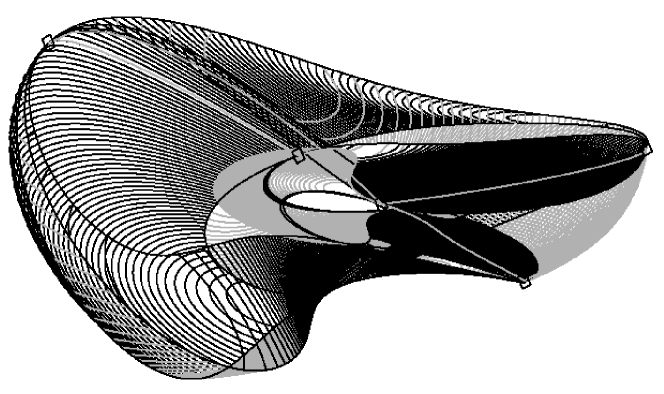
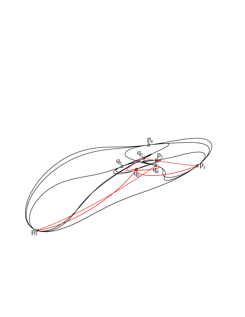
Figure 5. The solid torus $U$. On top, we have drawn all its $2$-faces, as well as its $1$-skeleton. On the bottom, only the $1$-skeleton with vertices labelled. These pictures are included only for motivational purposes, they are not needed in the proofs.

The Dirichlet domain has an arc in the boundary of a Giraud disk between $q_{1}$ and $q_{2}$, which is in the intersection of the faces $b_{4}$ and $b_{5}$. By Giraud’s theorem (see [10], p. 264), there are precisely three bisectors containing that Giraud disk, namely $\mathcal{B}_{4}$, $\mathcal{B}_{5}$, as well as

$$\mathcal{C}=\mathcal{B}(G_{1}^{-1}p_{0},G_{2}^{-1}G_{3}p_{0}).$$

One way to get a fundamental domain for the action of $G_{2}$ on $U$ is to intersect $U$ with the appropriate region between $\mathcal{C}$ and $G_{2}\mathcal{C}$, namely

$$D=\left\{z\in\mathbb{C}^{3}:|\langle z,G_{1}^{-1}p_{0}\rangle|\leqslant|\langle z,G_{2}^{-1}G_{3}p_{0}\rangle|,|\langle z,G_{3}p_{0}\rangle|\leqslant|\langle z,G_{2}G_{1}^{-1}p_{0}\rangle|\right\}$$

This turns out to give a slightly complicated fundamental domain (in particular it is not connected). We will only use $\mathcal{C}$ as a guide in order to get a simpler fundamental domain.

By construction, $\mathcal{C}$ contains $q_{1}$ and $q_{2}$. One easily checks by direct computation that it also contains $p_{2}$, which is given in homogeneous coordinates by $(0,0,1)$. To that end, one computes

$$\langle p_{2},G_{1}^{-1}p_{0}\rangle=\langle p_{2},G_{2}^{-1}G_{3}p_{0}\rangle=\frac{9+i\sqrt{7}}{4}.$$

One then studies the intersection of $\mathcal{C}$ with each face of $U$ by using the techniques of section 2.3. The only difficulty is that the relevant bisectors are not all coequidistant but their intersections turn out to be disks (this will be proved in section 10.4 of the appendix). The combinatorics of $\mathcal{C}\cap E$ is illustrated in Figure 6.

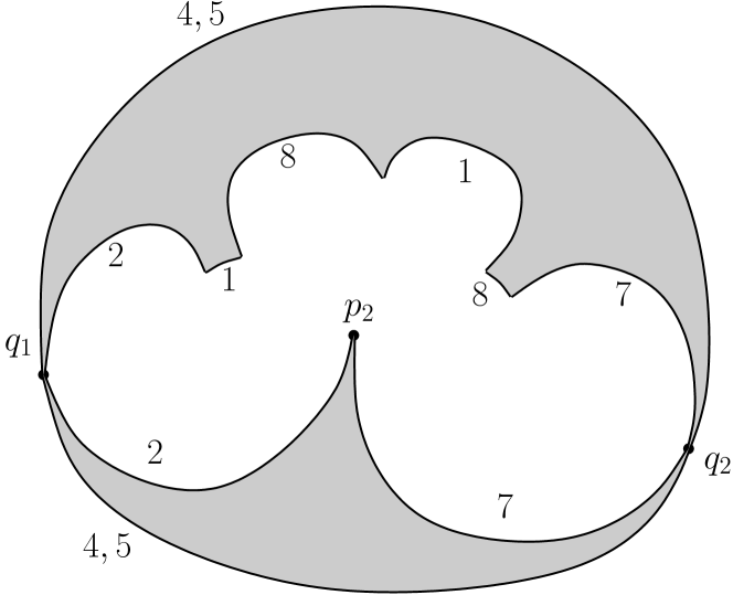
Figure 6. Combinatorics of the intersection of the spinal sphere $\partial_{\infty}\mathcal{C}$ with the solid torus $U$. The interior of this intersection has two components, one is a topological triangle with vertices $p_{2}$, $q_{1}$ and $q_{2}$.

The picture suggests a natural way to choose an explicit parametrized triangle $T$, with vertices $p_{2}$, $q_{1}$ and $q_{2}$ (and sides on the appropriate bisector intersections, as indicated by labels in Figure 6).

Propositions 6.2 and 6.3 give a precise definition of $T$ (their proof is quite computational, so we will give them in the appendix, sections 10.4-10.7).

Proposition 6.2.

1. $\partial_{\infty}(\mathcal{B}_{4}\cap\mathcal{B}_{5})$ is a topological circle containing $q_{1}$, $q_{2}$ and $p_{4}$. We denote by $\tau_{0}$ the arc from $q_{1}$ to $q_{2}$ not going through $p_{4}$.

2. $\partial_{\infty}(C\cap\mathcal{B}_{7})$ is a topological circle containing $q_{2}$ and $p_{2}$, and only one of the two arcs of that circle from $q_{2}$ to $p_{2}$ is entirely contained in $U$; we write $\tau_{1}$ for that arc.

3. $\partial_{\infty}(C\cap\mathcal{B}_{2})$ is a topological circle containing $q_{1}$ and $p_{2}$, and only one of the two arcs of that circle from $p_{2}$ to $q_{1}$ is entirely contained in $U$; we write $\tau_{2}$ for that arc.

4. The curve $\tau$ obtained by concatenating the arcs $\tau_{0}$, $\tau_{1}$ then $\tau_{2}$ from items (1), (2) and (3) is an embedded topological circle in $\partial_{\infty}C$.

Item (1) is obvious, since $\mathcal{B}_{4}\cap\mathcal{B}_{5}$ is a Giraud disk, and we know which vertices lie on it (see section 4.3). Items (2) and (3) follow from each other by symmetry, we will only justify (3). The latter is made plausible by Figure 7, which can be obtained using the parametrizations explained in section 2.3.

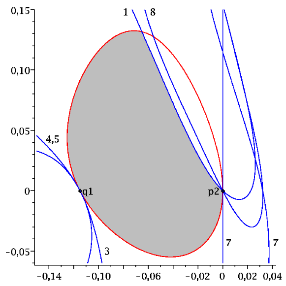
Figure 7. Combinatorics of the intersection of $\mathcal{C}\cap\mathcal{B}_{2}\cap E$.

Proposition 6.3.

The curve $\tau$ defined in Proposition 6.2 bounds a unique triangle $T$ in $\partial_{\infty}C$ that is properly embedded in $U$. Moreover, $T$ and $G_{2}^{2}T$ are disjoint.

An important consequence of Proposition 6.3 is the following.

Corollary 6.4.

$U$ is an embedded solid torus in $\partial_{\infty}{{\bf H}^{2}_{\mathbb{C}}}$.

Proof: The triangles $T$ and $G_{2}^{2}(T)$ split $U$ into two balls (they are indeed balls because they are bounded by topological embedded $2$-spheres), glued along two disjoint disks. From this it follows that $U$ is a solid torus. $\Box$

In order to get a simple fundamental domain, we will modify the meridian of Proposition 6.3 slightly.

Proposition 6.5.

The side $\tau_{1}$ (resp. $\tau_{2}$) of $T$ is isotopic in the boundary to the arc of $\mathbb{C}$-circle joining these two points on the face $b_{7}$ (resp. $b_{2}$). Moreover, this isotopy can be performed so that the corresponding sides of the triangle $G_{2}(T)$ intersect the boundary of $T$ precisely in $q_{2}$.

Proof: The combinatorics of the face $b_{2}$ are combinatorially the same as Figure 2, but the pinch points are $p_{1}$ and $q_{4}$, and the other two vertices are $p_{2}$ and $q_{1}$ (see Figure 4). Since $\tau_{2}$ is contained in the face $b_{2}$ and contains no other vertex than $q_{1}$ and $p_{2}$, it remains in the interior of the quadrilateral component of $b_{2}$. In that disk component, any two paths from $q_{1}$ to $p_{2}$ are isotopic, hence all of them are isotopic to the path that follows the (appropriate) arc of the $\mathbb{C}$-circle between these two points.

The argument for $\tau_{1}$ is similar. The fact that the isotopies for $T$ and $G_{2}(T)$ are compatible (in the sense that one can keep their sides disjoint throughout the isotopy) is obvious from the description of the combinatorics of $\partial U$, see Figure 8.

Figure 8. Isotopy of part of the boundary of $T$ and $G_{2}(T)$ towards an arc of a $\mathbb{C}$-circle.

$\Box$

The upshot of the above discussion is that we have a convenient choice of a meridian for the solid torus $U$, given by the concatenation of the following three arcs

• The arc of $\mathbb{C}$-circle from $p_{2}$ to $q_{1}$ which is the boundary of a slice of the face $b_{2}$ (only one such arc is contained in the Dirichlet domain);

• The arc of the boundary of the Giraud disk given by the intersection of the two bisectors $\mathcal{B}_{4}$ and $\mathcal{B}_{5}$, from $q_{1}$ to $q_{2}$ (there are two arcs on the boundary of this Giraud disk, we choose the one that does not contain $p_{4}$);

• The arc of $\mathbb{C}$-circle from $q_{2}$ to $p_{2}$ which is the boundary of a slice of the bisector $\mathcal{B}_{7}$ (only one such arc is contained in the Dirichlet domain).

We denote this curve by $\sigma$.

Proposition 6.6.

The curve $\sigma$ bounds a topological triangle $\tilde{T}$ which is properly contained in $U$. This triangle can be chosen so that $\tilde{T}\cap G_{2}\tilde{T}$ consists of a single point, namely $q_{2}$.

Proof: This follows from the properties of $T$ and the isotopy of Proposition 6.5. $\Box$

7. The manifold at infinity

The results from section 6 give a simple fundamental domain for the action of $\Gamma$ in the domain of discontinuity. For ease of notation, we denote $\tilde{T}$ simply by $T$, see section 6 for how to obtain this modified meridian for the solid torus $U$; recall that $U$ is by definition the boundary at infinity $\partial_{\infty}E$ of the Dirichlet domain $E$.

Definition 7.1.

Let $D$ be obtained from the portion of $U$ that is between $T$ and $G_{2}(T)$.

By construction, this region has ten faces, eight coming from the faces of the Dirichlet domain, and two given by $T$ and $G_{2}(T)$. For each $k=1,\dots,8$, we denote by

$$f_{k}=D\cap b_{k}$$

the portion of $b_{k}$ that is inside $D$.

By construction, $D\cup G_{2}D\cup G_{2}^{2}D\cup G_{2}^{-1}D$ is equal to the solid torus $U=\partial_{\infty}E$. Since we have proved that $E$ tiles ${{\bf H}^{2}_{\mathbb{C}}}$, $U$ tiles $\partial_{\infty}{{\bf H}^{2}_{\mathbb{C}}}$ (in the sense that eiher $U$ and $\gamma U$ coincide or $U\cap\gamma U$ has empty interior). A Heisenberg view of the $1$-skeleton of $D$ is illustrated in Figure 9, and a more combinatorial one, which we will use later, is given in Figure 10.

The pictures we get are not quite the same as Figure 1 (which is the one that usually appears in the literature on the figure eight knot), but they are obtained from it by taking the mirror image.

Note however that both oriented manifolds given by the usual or the opposite orientation of the figure eight knot complement admit a uniformizable spherical CR structure. Indeed, one can precompose the developing map by an orientation-reversing automorphism of the figure eight knot (hence the holonomy gets precomposed by the corresponding automorphism of the fundamental group), see section 9 for more details.

Figure 9. A Heisenberg view of the $1$-skeleton of the fundamental domain $D$.

Figure 10. The quotient manifold is homeomorphic to a ball with identifications on the boundary (one glues pairs of faces with matching arrows).

Setting $V=\{p_{1},\dots,p_{4},q_{1},\dots,q_{4}\}$, we also have that $U^{0}=U\setminus V$ tiles the set of discontinuity $\Omega$ (indeed, it follows from the Poincaré polyhedron theorem that the only fixed points of parabolic elements in the group are conjugate to either $p_{1}$ or $q_{1}$, see section 5). We analyze the quotient of $\Omega$ using the side pairings, which are given either by the action of $G_{2}$ or by the side pairings coming from the Dirichlet domain.

There are four side pairings, given in Table 3, three coming from the Dirichlet domain, and one given by $G_{2}$.

Proposition 7.2.

The maps $G_{1}$, $G_{2}$, $G_{3}$ and $G_{3}G_{1}$ give side pairings of the faces of $D$, and map the vertices according to Table 3.

$f_{4}$	$\stackrel{{\scriptstyle G_{1}}}{{\longrightarrow}}$	$f_{1}$
$p_{1},q_{2},q_{1}$		$p_{1},q_{3},p_{2}$

$f_{2}$	$\stackrel{{\scriptstyle G_{3}}}{{\longrightarrow}}$	$f_{7}$
$p_{1},p_{2},q_{1}$		$q_{3},p_{2},q_{2}$

$f_{3}$	$\stackrel{{\scriptstyle G_{3}G_{1}}}{{\longrightarrow}}$	$f_{8}$
$p_{1},q_{1}$		$q_{3},p_{2}$

$T$	$\stackrel{{\scriptstyle G_{2}}}{{\longrightarrow}}$	$G_{2}T$
$p_{2},q_{1},q_{2}$		$p_{1},q_{2},q_{3}$

Table 3. The four side pairings, with their action on vertices. We denote by $f_{k}$ the part of $\partial_{\infty}b_{k}$ that is contained in $D$.

Proof: The claim about $G_{2}$ holds by construction (see also Proposition 4.4). The ones about the other side pairings come from the Dirichlet domain (where an element $\gamma$ maps the face associated to $\gamma^{-1}$ to the face associated to $\gamma$), see section 5.1.

The claims about $G_{3}G_{1}$ follow from the previous ones, since

$$G_{3}G_{1}(p_{1})=G_{3}(p_{1})=q_{3}$$

and

$$G_{3}G_{1}(q_{1})=G_{3}(p_{2})=p_{2}.$$

$\Box$

We give a simple cut and paste procedure that allows us to identify the quotient as the figure eight knot complement, and this will conclude the proof of Theorem 1.1.

The procedure is illustrated in Figure 11. We slice off a ball bounded by $f_{7}$, $f_{8}$ as well as a triangle contained in the interior of $D$, and move it in order to glue it to face $f_{2}$ according to the side pairing given by $G_{3}^{-1}$. Now we group faces $f_{1}$ and $f_{8}$ on the one hand, and faces $f_{4}$ and $f_{3}$ on the other hand, and observe that their side pairings agree to give the identifications on the last domain in Figure 11. This is the same as Figure 1 (with the orientation reversed).

Figure 11. Cut and paste instructions for recovering the usual two-tetrahedra decomposition of the figure eight knot complement.

8. Relationship between $\Gamma_{2}$ and $\Gamma_{3}$

The goal of this section is to show that the groups $\Gamma_{2}$ and $\Gamma_{3}$ are conjugate subgroups of $\mathbf{PU}(2,1)$.

We write

$$G_{1}=\rho_{2}(g_{1}),\ G_{2}=\rho_{2}(g_{2}),\ G_{3}=\rho_{2}(g_{3})$$

and

$$A_{1}=\rho_{3}(g_{1}),\ A_{2}=\rho_{3}(g_{2}),\ A_{3}=\rho_{3}(g_{3}).$$

One can easily check that $A_{1}A_{3}^{-1}$ is regular elliptic element of order $4$, hence it is tempting to take its isolated fixed point as the center of a Dirichlet domain for $\Gamma_{3}$ (just like we did for $\Gamma_{2}$, using the fixed point of $G_{2}$).

In fact it is easy to see that the corresponging Dirichlet domain is isometric to that of $\Gamma_{2}$, and to deduce a presentation for $\Gamma_{3}$, say in terms of the generators $M=A_{1}A_{3}^{-1}$ and $N=A_{1}$:

$$\langle M,N|M^{4},(MN)^{3},(MNM)^{3}\rangle$$

With a little effort, these observations also produce an explicit conjugacy relation between both groups. Denote by $P$ the following matrix:

$$P=\left[\begin{matrix}1&0&0\\ \frac{-3-i\sqrt{7}}{4}&\frac{-5+i\sqrt{7}}{4}&0\\ \frac{-1+i\sqrt{7}}{2}&\frac{-1+i\sqrt{7}}{2}&2\end{matrix}\right]$$

Then one easily checks (most comfortably with symbolic computation software!) that

$$P^{-1}A_{1}P=G_{1}^{-1}G_{3}G_{1}$$

$$P^{-1}A_{3}P=G_{3}$$

Note that the above two matrices generate $\Gamma_{2}$. We will explain the precise relationship between the two representations $\rho_{2}$ and $\rho_{3}$ in section 9.

9. Action of $\textrm{Out}(\pi_{1}(M))$

The main goal of this section is to explain the relationship between the two representations $\rho_{2}$ and $\rho_{3}$, which turn out to differ by precomposition with an outer automorphism of $\pi_{1}(M)$. This is contained in the statement of Proposition 9.2, where we analyze the action of the whole outer automorphism group of $\pi_{1}(M)$.

We start by describing the outer automorphism group of $\pi_{1}(M)$ in terms of explicit generators (it is well known that this group is a dihedral group $D_{4}$ of order $8$). In fact $Out(\pi_{1}(M))$ can be visualized purely topologically in a suitable projection of the figure eight knot, for instance the one given in Figure 12.

Figure 12. A symmetric diagram for the figure eight knot - there are three planes of symmetry, one being the plane containing the projection.

The Wirtinger presentation (see [16] for instance) is given by

$$\langle x_{1},\dots,x_{4}\ |\ x_{4}x_{1}=x_{3}x_{4},\ x_{2}x_{3}=x_{3}x_{1},\ x_{3}x_{2}=x_{2}x_{4},\ x_{2}x_{1}=x_{1}x_{4}\ \rangle.$$

We eliminate $x_{2}$, then $x_{3}$ using

(10) $$x_{2}=x_{1}x_{4}x_{1}^{-1},\quad x_{3}=x_{2}x_{4}x_{2}^{-1}$$

and get

$$\langle x_{1},x_{4}\ |\ x_{4}[x_{1}^{-1},x_{4}]=[x_{1}^{-1},x_{4}]x_{1}\ \rangle.$$

It will be useful to observe that with this presentation, we can express

$$x_{3}=x_{1}x_{4}[x_{1}^{-1},x_{4}]x_{1}^{-1}=x_{1}[x_{1}^{-1},x_{4}]=x_{4}x_{1}x_{4}^{-1}.$$

Of course the above presentation is the same as the one given in section 3 if we set

$$x_{1}=g_{3}^{-1},\quad x_{4}=g_{1}^{-1}.$$

Using the Wirtinger presentation and an isotopy between the figure eight knot and its mirror image, for instance as suggested in Figure 13, one can check that the automorphisms described in Table 4 generate $\textrm{Out}(\pi_{1}(M))$.

Figure 13. An isotopy from the figure eight knot to its mirror image.

$$\sigma:\left\{\begin{array}[]{l}g_{1}\mapsto g_{3}\\ g_{3}\mapsto g_{1}\end{array}\right.\quad\iota:\left\{\begin{array}[]{l}g_{1}\mapsto g_{1}^{-1}\\ g_{3}\mapsto g_{3}^{-1}\end{array}\right.\quad\tau:\left\{\begin{array}[]{l}g_{1}\mapsto g_{1}^{-1}g_{3}g_{1}\\ g_{3}\mapsto g_{3}\end{array}\right.$$

Table 4. The three automorphisms $\sigma$, $\tau$, $\iota$ generate $Out(\pi_{1}(M))$.

Note that $\sigma$ and $\iota$ correspond to orientation-preserving diffeomorphisms (and they generate a group of order $4$), whereas $\tau$ reverses the orientation.

In what follows, for two representations $\rho$ and $\rho^{\prime}$, we write $\rho\sim\rho^{\prime}$ when the two representations are conjugate. We start with a very basic observation, valid for any unitary representation (not necessarily with Lorentz signature).

Proposition 9.1.

Let $\rho:\pi_{1}(M)\rightarrow\mathbf{U}(2,1)$. Then $\rho\circ\iota\sim\overline{\varphi}^{T}$.

Proof: For any element $A$ of $\mathbf{U}(2,1)$,

$$\overline{A}^{T}JA=J,$$

hence $A^{-1}=J^{-1}\ \overline{A}^{T}J$ is conjugate to $\overline{A}^{T}$. $\Box$

The precise relationship between $\rho_{2}$ and $\rho_{3}$ is as follows (we only give the action of $\textrm{Out}(\pi_{1}(M))$ on $\rho_{2}$, since the action on $\rho_{3}$ can easily be deduced from it).

Proposition 9.2.

Let $\varphi\in\textrm{Out}(\pi_{1}(M))$. Then

• $\rho_{2}\circ\varphi\sim\rho_{2}$ if and only if $\varphi$ is trivial or $\varphi=\sigma\iota$.

• $\rho_{2}\circ\varphi\sim\overline{\rho}_{2}$ if and only if $\varphi=\sigma$ or $\iota$.

• $\rho_{2}\circ\varphi\sim\rho_{3}$ if and only if $\varphi=\tau$ or $\iota\tau$.

• $\rho_{2}\circ\varphi\sim\overline{\rho}_{3}$ if and only if $\varphi=\sigma\iota\tau$ or $\sigma\tau$.

Proof: The fact that $\rho_{2}\circ\sigma\iota\sim\rho_{2}$ follows from the fact that $IG_{1}I=G_{3}^{-1}$, $IG_{3}I=G_{1}^{-1}$ (see section 4.1).

One easily checks that

(12) $$G_{1}^{T}=G_{3}^{-1},\quad G_{3}^{T}=G_{1}^{-1}.$$

Now the pair $G_{1}^{-1},G_{3}^{-1}$ is conjugate to $\overline{G}_{1}^{T},\overline{G}_{3}^{T}$ (because the matrices preserve $J$), which is conjugate to $\overline{G}_{3}^{-1},\overline{G}_{1}^{-1}$ (by (12)), which is conjugate to $\overline{G}_{1},\overline{G}_{3}$ (by conjugation by $I$). This shows that $\rho_{2}\circ\iota\sim\overline{\rho}_{2}$.

All that is left to prove is that $\rho_{2}\circ\tau\sim\rho_{3}$, and this was proved in section 8. $\Box$

10. Appendix - sample calculations

In this section we detail some of the computations that were mentioned in previous sections of the paper (the general computational strategy, and the geometric preliminaries are explained in section 2.3). Throughout the appendix, we denote by $\widehat{\mathcal{B}}_{j}$ denotes the extor in projective space extending $\mathcal{B}_{j}$ (see [10] for a definition and many properties of extors), and by $\overline{\mathcal{B}}_{j}$ the closure of $\mathcal{B}_{j}$ in ${\overline{\bf H}^{2}_{\mathbb{C}}}$. In other words, $\overline{\mathcal{B}}_{j}=\mathcal{B}_{j}\cup\partial_{\infty}\mathcal{B}_{j}$. More generally, $\widehat{O}$ denotes the extension to projective space of $O$, and $\overline{O}$ denotes its closure in ${\overline{\bf H}^{2}_{\mathbb{C}}}$.

10.1. Pairs of bounding bisectors - proof of Lemma 4.6

The center of the Dirichlet domain is given by

$$p_{0}=(1,-\frac{3+i\sqrt{7}}{4},-1).$$

Its relevant orbit points are given by

$$r_{1}=G_{1}p_{0}=(\frac{3+i\sqrt{7}}{4},\frac{1-i\sqrt{7}}{4},-1),\quad r_{2}=G_{3}^{-1}p_{0}=(1,\frac{1-i\sqrt{7}}{4},\frac{-3-i\sqrt{7}}{4})$$

$$r_{3}=G_{2}r_{1}=(2,\frac{-1-i\sqrt{7}}{2},\frac{-3-i\sqrt{7}}{4}),\quad r_{4}=G_{2}r_{2}=(\frac{9-i\sqrt{7}}{4},\frac{-7-i\sqrt{7}}{4},-1)$$

$$r_{5}=G_{2}^{2}r_{1}=(\frac{9-i\sqrt{7}}{4},\frac{-5-i\sqrt{7}}{2},-2),\quad r_{6}=G_{2}^{2}r_{2}=(2,\frac{-5-i\sqrt{7}}{2},\frac{-9+i\sqrt{7}}{4})$$

$$r_{7}=G_{2}^{-1}r_{1}=(1,\frac{-7-i\sqrt{7}}{4},\frac{-9+i\sqrt{7}}{4}),\quad r_{8}=G_{2}^{-1}r_{2}=(\frac{3+i\sqrt{7}}{4},\frac{-1-i\sqrt{7}}{2},-2).$$

The Giraud torus $\overline{\mathcal{B}}_{j}\cap\overline{\mathcal{B}}_{k}$ can be parametrized by using the techniques of section 2.3. We start by proving Lemma 4.6.

In order to show that $\mathcal{B}_{1}\cap\mathcal{B}_{2}$ is a disk, it is enough to exhibit a single point inside it, for instance

(13) $$X_{12}=(p_{0}-r_{1})\boxtimes(p_{0}-r_{2})=(\frac{1+i\sqrt{7}}{4},\frac{3-i\sqrt{7}}{8},-\frac{1+i\sqrt{7}}{4})$$

does the job, since $\langle X_{12},X_{12}\rangle=-3/4$. Similarly, $\mathcal{B}_{1}\cap\mathcal{B}_{3}$ is a disk, because

$$X_{13}=(p_{0}-r_{1})\boxtimes(p_{0}-r_{3})=(\frac{5+i\sqrt{7}}{8},\frac{3-i\sqrt{7}}{8},-\frac{1+i\sqrt{7}}{4})$$

satisfies $\langle X_{13},X_{13}\rangle=-1/2$.

In order to show that $\mathcal{B}_{1}\cap\mathcal{B}_{5}$ is empty, we parametrize the Giraud torus $\overline{\mathcal{B}}_{1}\cap\overline{\mathcal{B}}_{5}$ by vectors of the form $(\overline{z}_{1}p_{0}-r_{1})\boxtimes(\overline{z}_{2}p_{0}-r_{5}),$ so that $V(z_{1},z_{2})$ is given by $v_{0}+z_{1}v_{1}+z_{2}v_{2}$, where

$$v_{0}=(\frac{9-3i\sqrt{7}}{8},\frac{3+3i\sqrt{7}}{4},3),\quad v_{1}=v_{2}=(\frac{3-i\sqrt{7}}{8},-\frac{1+i\sqrt{7}}{4},-1),$$

see equation (3). We then write out

$$\langle V(z_{1},z_{2}),V(z_{1},z_{2})\rangle=\Re(\mu(z_{1})z_{2})-\nu(z_{1}),$$

where

$$\mu(z_{1})=\frac{5}{2}(\overline{z}_{1}-3),\quad\nu(z_{1})=-\frac{55}{4}+\frac{15}{2}\Re(z_{1}).$$

It is easy to verify that $\nu^{2}-|\mu|^{2}$ is always positive for $|z_{1}|=1$, for instance by writing $z_{1}=x+iy$, and computing

$$\nu(z_{1})^{2}-|\mu|^{2}=225(2x-3)^{2}/16.$$

Note that in order to get the previous formula, we have used the fact that $|z_{1}|^{2}=x^{2}+y^{2}=1$.

10.2. Proof of Lemma 4.7

We first treat the proof of part (1) of Lemma 4.7; even though, strictly speaking, it will not be needed in the proof, we strongly suggest that the reader keep Figure 3 in mind. We work only with $\mathcal{B}_{1}\cap\mathcal{B}_{7}$, since $\mathcal{B}_{1}\cap\mathcal{B}_{3}$ can be deduced from it by symmetry.

The Giraud torus $\widehat{\mathcal{B}}_{1}\cap\widehat{\mathcal{B}}_{7}$ can be parametrized by vectors of the form $(\overline{z}_{1}p_{0}-r_{1})\boxtimes(\overline{z_{2}}p_{0}-r_{7})$, with $|z_{1}|=|z_{2}|=1$. In other words, we normalize it to be the Clifford torus.

Explicitly, this can be written as $V(z_{1},z_{2})=v_{0}+z_{1}v_{1}+z_{2}v_{2}$, where

$$v_{0}=(\frac{9-3i\sqrt{7}}{8},\frac{-9+3i\sqrt{7}}{8},\frac{15+3i\sqrt{7}}{8})$$

$$v_{1}=(-1,\frac{5+i\sqrt{7}}{4},\frac{3-i\sqrt{7}}{8})$$

$$v_{2}=(\frac{-3+i\sqrt{7}}{8},\frac{-1-i\sqrt{7}}{4},-1)$$

The Giraud disk inside the Clifford torus is described by imposing that the above vector $V=V(z_{1},z_{2})$ be negative, i.e. $\langle V,V\rangle<0$ which can be written as

(14) $$\Re\left(7+\frac{-15-3i\sqrt{7}}{4}z_{1}+\frac{-15+3i\sqrt{7}}{4}z_{2}+\frac{i\sqrt{7}}{2}z_{1}\overline{z}_{2}\right)<0$$

The equations of the intersection with $\widehat{\mathcal{B}}_{j}$, $j=1,\dots,8$ are given by

(15) $$|\langle V(z_{1},z_{2}),p_{0}\rangle|^{2}=|\langle V(z_{1},z_{2}),r_{j}\rangle|^{2},$$

and we write them in simplified form in Table 5 (by simplified, we mean that we use $|z_{1}|=|z_{2}|=1$).

$\mathcal{B}_{1}$	$0$
$\mathcal{B}_{2}$	$\Re(-43+(-12+12i\sqrt{7})z_{1}+(33-3i\sqrt{7})z_{2}+(9-5i\sqrt{7})z_{1}\overline{z}_{2})\,/\,8$
$\mathcal{B}_{3}$	$\Re(-{81}+{54}z_{2})\,/\,8$
$\mathcal{B}_{4}$	$\Re(-{151}+(60+12i\sqrt{7})z_{1}+(60-12i\sqrt{7})z_{2}-(9+5i\sqrt{7})z_{1}\overline{z}_{2})\,/\,8$
$\mathcal{B}_{5}$	$\Re(-{81}+{54}z_{1})\,/\,8$
$\mathcal{B}_{6}$	$\Re(-{43}+(33+3i\sqrt{7})z_{1}-(12+12i\sqrt{7})z_{2}+(9-5i\sqrt{7})z_{1}\overline{z}_{2})\,/\,8$
$\mathcal{B}_{7}$	$0$
$\mathcal{B}_{8}$	$\Re(-16+(15+3i\sqrt{7})z_{1}+(15-3i\sqrt{7})z_{2}-(9+5i\sqrt{7})z_{1}\overline{z}_{2})\,/\,8$

Table 5. The equations of the intersection of each $\widehat{\mathcal{B}}_{j}$ with the Giraud torus containing $\widehat{\mathcal{B}}_{1}\cap\widehat{\mathcal{B}}_{7}$ (the Giraud torus is given by the Clifford torus $|z_{1}|=|z_{2}|=1$).

Proposition 10.1.

For $j=3,4$ and $5$, $\mathcal{B}_{j}$ does not intersect $\mathcal{B}_{1}\cap\mathcal{B}_{7}$.

Proof: This was already proved for $\widehat{\mathcal{B}}_{3}$ and $\widehat{\mathcal{B}}_{5}$, since we proved Lemma 4.6 in section 10.1 (is says that $\mathcal{B}_{1}\cap\mathcal{B}_{3}$ and $\mathcal{B}_{1}\cap\mathcal{B}_{5}$ are empty). Alternatively, this can also be recovered from the equations given in Table 5. For instance, the equation

$$-81+27(z_{2}+\overline{z}_{2})=0$$

has only one solution given by $z_{2}=3/2$, which is not on the unit circle.

We claim that the intersection with $\widehat{\mathcal{B}}_{4}$ is empty as well. One way to see this is to write the equation in the form

$$\Re(\mu(z_{1})z_{2})=\nu(z_{1}),$$

which has a solution $z_{2}$ with $|z_{2}|=1$ if and only if $|\nu(z_{1})|\leq|\mu(z_{1})|$.

In the case at hand,

$$\mu(z_{1})=\frac{15-3i\sqrt{7}}{2}+\frac{-9+5i\sqrt{7}}{8}\overline{z}_{1},\quad\nu(z_{1})=\frac{151}{8}-\Re\left(\frac{15+3i\sqrt{7}}{2}z_{1}\right).$$

One computes

$$\nu^{2}-|\mu|^{2}=18193/64-2025x/8+405\sqrt{7}y/8-42xy\sqrt{7}/2+(209x^{2}+47y^{2})/4,$$

where we have written $z_{1}=x+iy$. It is now standard 2-variable calculus to prove that this function is strictly positive on the unit disk. $\Box$

The extors $\widehat{\mathcal{B}}_{2}$, $\widehat{\mathcal{B}}_{6}$ and $\widehat{\mathcal{B}}_{8}$ have 1-dimensional intersection with the Giraud torus $\widehat{\mathcal{B}}_{1}\cap\widehat{\mathcal{B}}_{7}$. For the general description of their (piecewise) parametrization by one spinal coordinate, see section 2.3. We explicit the parametrization for $\widehat{\mathcal{B}}_{8}$, since this will be needed in later calculations.

The equation for the trace on the Clifford torus of $\widehat{\mathcal{B}}_{8}$ can be written as

$$\Re(\mu(z_{1})z_{2})=\nu(z_{1}),$$

where

$$\mu(z_{1})=\frac{15-3i\sqrt{7}}{8}+\frac{-9+5i\sqrt{7}}{8}\overline{z}_{1},\quad\nu(z_{1})=2-\Re\left(\frac{15+3i\sqrt{7}}{8}z_{1}\right)$$

Endpoints of the set of valid parameters are solutions of $|\mu|^{2}=\nu^{2}$, which is a real expression involving $z_{1}$, $\overline{z}_{1}$. Writing $z_{1}=x+iy$, we can write $\nu^{2}-|\mu|^{2}=h(x,y)$ where

$$h(x,y)=-1/2-45xy\sqrt{7}/32-(31x^{2}+193y^{2})/64.$$

The endpoint of the parametrization are solutions of $h(x,y)=0$ that satisfy $x^{2}+y^{2}=1$. The corresponding system has two solutions given by $z_{1}=x+iy=\pm(5-i\sqrt{7})/4\sqrt{2}$, which have $\arg(z_{1})/(2\pi)$ approximately equal to $-0.07745991$ and $0.42254009$ (compare with the abscissas of the double points in Figure 14).

Between these two values of the arguments, the sign of the discriminant $\nu^{2}-|\mu|^{2}$ does not change, and it can easily be checked that it is in fact nonpositive everywhere. In other words, the formulae given in (7) parameterize the entire trace of $\widehat{\mathcal{B}}_{8}$ on the Clifford torus. The corresponding curve is depicted in Figure 14 (the figure is given only as a guide, it is not needed in the proof).

Figure 14. The trace of $\mathcal{B}_{8}$ on the Giraud torus $\mathcal{B}_{1}\cap\mathcal{B}_{7}$, in terms of the log of the spinal coordinates (the bold oval is the boundary at infinity of the Giraud disk).

Note that the curve seems to contain a straight line of slope one. This is indeed the case, and it corresponds to a curve of the form $z_{2}=\tau z_{1}$, for some complex number $\tau$ with $|\tau|=1$. This straight line is actually contained in a complex slice of the third bisector in Giraud’s theorem, namely $\mathcal{B}(r_{1},r_{7})$. Using the explicit form of the equation, plugging $z_{2}=\tau z_{1}$, one finds a unique value of $\tau$ such that the equation becomes trivial, namely

(16) $$\tau=-\frac{9+5i\sqrt{7}}{16}.$$

It is easy to see that this curve lies entirely outside complex hyperbolic space. In fact substituting $z_{2}=\tau z_{1}$ in (14) (and using $|z_{1}|=1$) yields a constant, namely $189/32$, which is positive.

Proposition 10.2.

For $j=2$, $6$ and $8$, $\mathcal{B}_{j}$ does not intersect $D=\mathcal{B}_{1}\cap\mathcal{B}_{7}$. In terms of their closures in ${\overline{\bf H}^{2}_{\mathbb{C}}}$, we have the following:

• $\overline{\mathcal{B}}_{2}\cap\overline{D}=\{p_{2}\}$, which is the fixed point of $G_{3}$;

• $\overline{\mathcal{B}}_{6}\cap\overline{D}=\{q_{3}\}$, which is the fixed point of $G_{1}G_{2}^{-1}$;

• $\overline{\mathcal{B}}_{8}\cap\overline{D}=\{p_{2},q_{3}\}$.

Moreover, (the extensions to projective space of) all these curves are tangent to $\partial_{\infty}D$ at every intersection point.

Proof: For $j=6$ and $7$, this follow from Proposition 4.4 and Theorem 2.3 (since $\mathcal{B}_{1}$, $\mathcal{B}_{6}$, resp. $\mathcal{B}_{2}$, $\mathcal{B}_{7}$, have tangent spinal spheres).

The statement about $j=8$ is a bit more difficult. We work in the Giraud torus normalized as the Clifford torus, which we write as $\widehat{D}$. We prove that the curves defined on $\widehat{D}$ by the equations for $\widehat{\mathcal{B}}_{2}$ and $\widehat{\mathcal{B}}_{8}$ are tangent at $p_{2}$ (a similar argument shows that the curves defined $\widehat{\mathcal{B}}_{6}$ and $\widehat{\mathcal{B}}_{8}$ are tangent at $q_{3}$).

Recall that $p_{2}=(0,0,1)$, which we now need to write in the spinal coordinates $(z_{1},z_{2})$ for $\widehat{D}$. This is done by solving $\langle p_{2},\overline{z}_{1}p_{0}-r_{1}\rangle=0$ for $z_{1}$, and $\langle p_{2},\overline{z}_{2}p_{0}-r_{2}\rangle=0$ for $z_{2}$. Explicit calculation shows $p_{2}$ is given in spinal coordinates by

$$(z_{1},z_{2})=(\frac{3-i\sqrt{7}}{4},1).$$

All equations in Table 5 have the form $f=0$ where

$$f(z_{1},z_{2})=2\Re(a_{0}+a_{1}z_{1}+a_{2}z_{2}+a_{12}z_{1}\overline{z}_{2}).$$

Since we are interested in the solution set only on the Clifford torus, we write $z_{1}=e^{it_{1}}$ and $z_{2}=e^{it_{2}}$ for real $t_{j}$. the gradient of $f$, seen as a function of $(t_{1},t_{2})$ is then given by

$$\frac{\partial f}{\partial t_{1}}=-2\Im(a_{2}z_{2}+\overline{a}_{12}\overline{z}_{1}z_{2}),\qquad\frac{\partial f}{\partial t_{2}}=-2\Im(a_{2}z_{2}+\overline{a}_{12}\overline{z}_{1}z_{2}).$$

This gives

$$\nabla f_{2}(\frac{3-i\sqrt{7}}{4},1)=(-\frac{3\sqrt{7}}{4},-\frac{3\sqrt{7}}{8}),\qquad\nabla f_{8}(\frac{3-i\sqrt{7}}{4},1)=(\frac{3\sqrt{7}}{8},\frac{3\sqrt{7}}{16}),$$

where $f_{j}$ denotes the equation of $\mathcal{B}_{j}\cap\widehat{D}$, see Table 5. This shows the needed tangency.

It follows from Proposition 2.3 that $\widehat{\mathcal{B}}_{2}\cap\widehat{D}$ is tangent to $\partial_{\infty}D$ at $p_{2}$. From the previous computation, we see that $\widehat{\mathcal{B}}_{2}\cap\widehat{D}$ is also tangent to $\partial_{\infty}D$ at $p_{2}$.

We now argue that $\widehat{\mathcal{B}}_{8}\cap\widehat{D}=\{p_{2},q_{3}\}$. Even though this is quite clear from the picture of the parametrized curve, we give a computational argument that does not rely on visual aids.

We have explicit equations for $\partial_{\infty}D$ and $\widehat{\mathcal{B}}_{8}$, namely (14) (with the inequality replaced by an equality) and (15). Writing out $z_{j}=x_{j}+iy_{j}$ for real $x_{j},y_{j}$, the intersection $\partial_{\infty}D\cap\widehat{\mathcal{B}}_{8}$ is described by the solutions of the system

$$\left\{\begin{array}[]{l}15(x_{1}+x_{2})+3\sqrt{7}(y_{2}-y_{1})+2\sqrt{7}(x_{2}y_{1}-y_{2}x_{1})=28\\ 15(x_{1}+x_{2})+3\sqrt{7}(y_{2}-y_{1})-9(x_{1}x_{2}+y_{1}y_{2})+5\sqrt{7}(x_{2}y_{1}-y_{2}x_{1})=16\\ x_{1}^{2}+y_{1}^{2}=1\\ x_{2}^{2}+y_{2}^{2}=1\end{array}\right.$$

One checks that this has exactly two solutions, given by $(z_{1},z_{2})=(1,\frac{3+i\sqrt{7}}{4})$ (this corresponds to $q_{3}$) and $(z_{1},z_{2})=(\frac{3-i\sqrt{7}}{4},1)$ (this corresponds to $p_{2}$).

Recall that $\widehat{D}\cap\widehat{\mathcal{B}}_{8}$ contains a diagonal component, given by $z_{2}=\tau z_{1}$ with $\tau$ as in (16). Recall that $\widehat{D}\cap\widehat{\mathcal{B}}_{8}$ has two double points, which were computed on page 10.2. Away from these two endpoints, for a given $z_{1}\in S^{1}$, there is precisely one point $(z_{1},z_{2})$ in $\widehat{D}\cap\widehat{\mathcal{B}}_{8}$ that is not in the diagonal component. The closure of that component (obtained by adding the two double points), gives an embedded topological circle in $\widehat{D}$. Since its only contact points with $\partial_{\infty}D$ are the two tangency points, we know this circle lies entirely outside $D$. $\Box$

This finishes the proof of part (1) of Lemma 4.7. Part (2) is very similar; by symmetry, it is enough to consider $\mathcal{B}_{1}\cap\mathcal{B}_{2}$.

As in the case of $\mathcal{B}_{2}\cap\mathcal{B}_{7}$, one finds all the intersections of the Giraud torus $\overline{\mathcal{B}}_{1}\cap\overline{\mathcal{B}}_{2}$ with every $\overline{\mathcal{B}}_{k}$ ($k\neq 1,2$), and checks that the only ones are given by $p_{1}$, $p_{2}$ and $q_{4}$. This shows that $\mathcal{B}_{1}\cap\mathcal{B}_{2}\cap E$ is either empty or all of $\mathcal{B}_{1}\cap\mathcal{B}_{2}$. One shows that it is a disk simply by finding one point in it, for instance the point in (13) is easily seen to be inside $E$ by computing six inequalities.

This finishes the proof of Lemma 4.7, hence also of part (1) of Proposition 4.5. Part (2) will be proved in section 10.3.

10.3. Spinal sphere of $\mathcal{B}_{1}$ - proof of Proposition 4.5(2)

In this section, we justify Proposition 4.5(2); in other words, we justify the picture given in Figure 2.

We start by giving explicit coordinates on $\mathcal{B}_{1}=\mathcal{B}(p_{0},G_{1}p_{0})$. We choose coordinates for ${{\bf H}^{2}_{\mathbb{C}}}$, seen as the unit ball $\mathbb{B}^{2}\subset\mathbb{C}^{2}$, where the midpoint of the segment $[p_{0},r_{1}]$ is taken to be at the origin of the ball (as in section 10.1, we write $r_{1}=G_{1}p_{0}$). Since $\langle p_{0},r_{1}\rangle$ is real (and $\langle p_{0},p_{0}\rangle=\langle r_{1},r_{1}\rangle$), the midpoint is given by $p_{0}+r_{1}$, and an orthogonal vector spanning the complex spine is given by $p_{0}-r_{1}$.

We normalize these vectors to have unit norm, so we take

$$v_{0}=(p_{0}+r_{1})/\sqrt{5}=(\frac{7+i\sqrt{7}}{4\sqrt{5}},\frac{-1-i\sqrt{7}}{2\sqrt{5}},-\frac{2}{\sqrt{5}}),$$

$$v_{1}=p_{0}-r_{1}=(\frac{1-i\sqrt{7}}{4},-1,0),$$

$$v_{2}=(\frac{-3+i\sqrt{7}}{4\sqrt{5}},-\frac{1+i\sqrt{7}}{2\sqrt{5}},-\frac{2}{\sqrt{5}}).$$

The last vector is chosen so that $v_{0},v_{1},v_{2}$ is a standard Lorentz basis, i.e. if $P$ denotes the corresponding base change matrix,

$$P^{*}JP=\left(\begin{matrix}-1&0&0\\ 0&1&0\\ 0&0&1\end{matrix}\right).$$

We now work in $\mathbb{C}^{2}$, with affine coordinates $u_{1}=z_{1}/z_{0}$, $u_{2}=z_{2}/z_{0}$, where the $z_{j}$ denote coordinates in the basis $v_{0},v_{1},v_{2}$; the complex hyperbolic plane ${{\bf H}^{2}_{\mathbb{C}}}$ is then simply given by the unit ball $|u_{1}|^{2}+|u_{2}|^{2}<1$.

The ball coordinates for $p_{0}$ and $r_{1}$ are given by $(\pm 1/\sqrt{5},0)$, and the bisector $\mathcal{B}_{1}$ has a very simple equation, namely

$$\Re(u_{1})=0,$$

so the bisector can simply be thought of as the unit ball in $\mathbb{R}^{3}$, when using coordinates $(t_{1},t_{2},t_{3})$ for a point in $\mathbb{B}^{2}$ of the form

$$(it_{3},t_{1}+it_{2}).$$

Here we have choosen the real spine of $\mathcal{B}_{1}$ to be given by the last coordinate axis.

The equation of the intersection of a bisector $\mathcal{B}_{j}=\mathcal{B}(p_{0},r_{j})$ for some $j>1$ is obtained simply by writing $r_{j}$ in the new basis. In fact the equation has the form

(17) $$|\langle Z,P^{-1}p_{0}\rangle|^{2}=|\langle Z,P^{-1}r_{j}\rangle|^{2}$$

where one takes $Z=(1,it_{3},t_{1}+it_{2})$.

We write $g_{j}$ for the equation of $\widehat{\mathcal{B}}_{2}\cap\partial_{\infty}\mathcal{B}_{1}$ in the coordinates $t_{j}$ for $\partial_{\infty}\mathcal{B}_{1}$ described above. According to previous discussions (see section 4.3), we only need to consider the bisectors $\widehat{\mathcal{B}}_{2}$ and $\widehat{\mathcal{B}}_{8}$. The affine coordinates of $r_{2}$ and $r_{8}$ are given by

$$(0,\frac{-9+5i\sqrt{7}}{24}),\quad(0,\frac{2}{3}),$$

respectively.

We consider the intersection of $\widehat{\mathcal{B}}_{j}$ with $\partial_{\infty}\mathcal{B}_{1}$, the latter being given by the unit sphere $t_{1}^{2}+t_{2}^{2}+t_{3}^{2}=1$. Computationally, we take the resultant $h_{j}$ of $g_{j}$ and $t_{1}^{2}+t_{2}^{2}+t_{3}^{2}-1$ with respect to $t_{3}$. For $j=2$ and $8$ we get

$$h_{2}(t_{1},t_{2})=\frac{21}{20}\{(t_{1}+\frac{9}{14})^{2}+(t_{2}-~\frac{5}{2\sqrt{7}})^{2}-\frac{50}{49}\},\quad h_{8}(t_{1},t_{2})=\frac{21}{20}\{(t_{1}-\frac{8}{7})^{2}-t_{2}^{2}-\frac{50}{49}\}.$$

The equations $h_{2}=0$ and $h_{8}=0$ define two cylinders in $\mathbb{R}^{3}$, that project to a pair of tangent circles. The point of tangency of the projections is given by $(1/4,5\sqrt{7}/28)$, as illustrated in Figure 15.

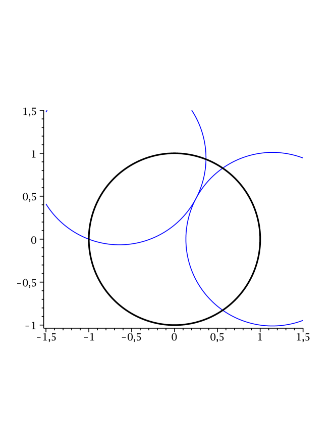
Figure 15. When $\mathcal{B}_{1}$ is normalized to be the unit ball with real spine given by the $t_{3}$-axis, $\mathcal{B}_{1}\cap\mathcal{B}_{2}$ and $\mathcal{B}_{1}\cap\mathcal{B}_{8}$ project to circles in the $(t_{1},t_{2})$-plane.

The inequalities defining the Dirichlet domain correspond to $g_{j}$ being negative. In particular, points in the interior of the Dirichlet domain are the points in the unit ball that project outside both these circles.

It follows from the analysis in section 4.3 and the results in section 10.2 that $\partial_{\infty}b_{1}$ is bounded only by the two curves corresponding to the intersections with $\mathcal{B}_{2}$ and $\mathcal{B}_{8}$ (both of these curves are traces on the $\partial_{\infty}{{\bf H}^{2}_{\mathbb{C}}}$ of Giraud disks). This finishes the proof of Proposition 4.5.

10.4. The intersection $C\cap\mathcal{B}_{2}$ is a disk

In this section we consider $C\cap\mathcal{B}_{2}$, where $C=\mathcal{B}(G_{1}^{-1}p_{0},G_{2}^{-1}G_{3}p_{0})=\mathcal{B}(r_{4},r_{5})$. We will show that it is a disk.

Note that these the bisectors $C$ and $\mathcal{B}_{2}$ do not share any complex slice, i.e. their extended real spines do not intersect. This amounts to saying that the circles $\overline{z}_{1}r_{4}-r_{5}$, $|z_{1}|=1$ and $\overline{z}_{1}p_{0}-r_{2}$, $|z_{2}|=1$ do not intersect.

One way to see this is to compute the intersection of their extended complex spine, which can be represented by

$$s=(-3\sqrt{7}-5i,\ 4\sqrt{7}+10i,\ 4\sqrt{7}),$$

and to note that this vector satisfies $\langle s,s\rangle=44>0$. This point is on the real spine of $C$ if and only if there exists a $z_{1}\in S^{1}$ such that $\langle s,\overline{z}_{1}r_{4}-r_{5}\rangle=0$. The latter can only happen if $z_{1}=(9+15i\sqrt{7})/46$, but this does not have modulus one. Similarly one checks that $s$ is not on the real spine of $\mathcal{B}_{2}$.

Now the intersection $C\cap\mathcal{B}_{2}$ can be parametrized by vectors of the form $(\overline{z}_{1}r_{4}-r_{5})\boxtimes(\overline{z}_{2}p_{0}-r_{2})$. Such vectors have negative norm if and only if

(18) $$\Re(\mu(z_{1})z_{2})<\nu(z_{1})$$

where

$$\mu(z_{1})=(-39-3i\sqrt{7}+(9+3i\sqrt{7})z_{1}+18\overline{z}_{1})/4,\quad\nu(z_{1})=-15+\Re\{(24+3i\sqrt{7})z_{1}\}/2.$$

In order to analyze the number of connected components of the intersection, we search for values of $z_{1}$ where the discriminant vanishes. Writing $z_{1}=x+iy$, the discriminant $\nu(z_{1})^{2}-|\mu(z_{1})|^{2}$ becomes

$$\delta(x,y)=(1413-1764x+216\sqrt{7}y+351(x^{2}-y^{2})-180\sqrt{7}xy)/8,$$

The system $\delta(x,y)=x^{2}+y^{2}-1=0$ has exactly two solutions, one given by $(x,y)=(1,0)$, and the other one given by the single real root of each of the polynomials $2221x^{3}-7103x^{2}+7411x-2473$, $392\sqrt{7}+2268y+1024\sqrt{7}y^{2}+2221y^{2}$. An approximate value of $(x,y)$ is $(0.70552301,-0.70868701)$.

In fact only the number of solutions interests us; $z_{1}=e^{2\pi it_{1}}$ give nontrivial intervals of values of $z_{2}$ when $t_{1}^{min}<t_{1}<0$, where $t_{1}^{min}=-0.12535607\dots$. For each such $z_{1}$, there is only an interval of values of $z_{2}$ satisfying (18), hence $C\cap\mathcal{B}_{2}$ is a disk.

10.5. Proof of Proposition 6.2(3)

We consider the segment $\tau_{2}$, which corresponds to the bottom segment from $q_{1}$ to $p_{2}$ shown on Figure 7. We prove that it is contained in the (boundary at infinity of the) Dirichlet domain; this will prove Proposition 6.2, since one easily shows that the top arc of Figure 7 is not contained in $U$, simply by picking one point just above $p_{2}$.

It is enough to find all intersection points of $C\cap\mathcal{B}_{2}\cap\mathcal{B}_{j}$ for $j\neq 2$, and to show that none of them is in (the interior of) the bottom segment; note that, in our coordinates, the bottom segment is characterized by the fact that $\arg(z_{2})<0$.

The (finite) list of points in $C\cap\mathcal{B}_{2}\cap\mathcal{B}_{j}$ can be obtained by using Groebner bases. For instance, for $j=1$, the intersection points are given by the solutions of the system

$$\left\{\begin{array}[]{l}-\frac{99}{8}-\frac{3\sqrt{7}}{2}y_{1}+\frac{21}{2}x_{1}-\frac{3}{2}x_{1}+\frac{15\sqrt{7}}{8}(x_{1}y_{2}+y_{1}x_{2})+\frac{27}{8}(x_{1}x_{2}-y_{1}y_{2})=0\\ 15-12x_{1}+\frac{3\sqrt{7}}{2}y_{1}-\frac{39}{4}x_{2}+\frac{3\sqrt{7}}{4}y_{2}+\frac{27}{4}x_{1}x_{2}+\frac{9}{4}y_{1}y_{2}-\frac{3\sqrt{7}}{4}(x_{1}y_{2}+x_{2}y_{1})=0\\ x_{1}^{2}+y_{1}^{2}=1\\ x_{1}^{2}+y_{2}^{2}=1\end{array}\right.$$

where we have split $z_{1}=x_{1}+iy_{1}$ and $z_{2}=x_{2}+iy_{2}$ into their real and imaginary parts. This system has precisely two solutions, one given by $(z_{1},z_{2})=(1,0)$, and the other one with

$$\arg(z_{1})/(2\pi)\approx-0.06508170,\quad\arg(z_{2})/(2\pi)\approx 0.13166662$$

For $j=3$, the result follows from direct calculations in a similar vein (using Groebner bases in order to solve the system). The intersection of $\mathcal{B}_{3}$ is tangent to $\partial_{\infty}(C\cap\mathcal{B}_{2})$, so one gets a single intersection point, corresponding to $q_{1}$.

For $j=5$ or $7$, no computation is needed; we already know that $\mathcal{B}_{2}\cap\mathcal{B}_{5}=\{q_{1}\}$ and $\mathcal{B}_{2}\cap\mathcal{B}_{7}=\{p_{2}\}$, since the corresponding bisectors have tangent spinal spheres (see section 4).

Remark 10.3.

The intersections $C\cap\mathcal{B}_{2}\cap\mathcal{B}_{j}$ can also be handled by using coequidistant pairs of bisectors, by writing the equation of the trace of $C$ on $\mathcal{B}_{2}\cap\mathcal{B}_{j}$.

10.6. Proof of Proposition 6.2(4)

In this section, we prove that the curve $\tau$ from Proposition 6.2 is an embedded topological circle in $\partial_{\infty}C$. We also give explicit parametrizations of its sides $\tau_{0}$, $\tau_{1}$, $\tau_{2}$, which are used to draw the pictures in section 10.7.

We start by parametrizing $\partial_{\infty}C$; we choose coordinates for ${{\bf H}^{2}_{\mathbb{C}}}$ (seen as the unit ball $\mathbb{B}^{2}$) where the midpoint of $[r_{4},r_{5}]$ is at the origin (such a normalization was already discussed in section 10.3). A possible base change matrix is given by

(19) $$P=\left(\begin{matrix}\frac{9-i\sqrt{7}}{2\sqrt{5}}&0&\frac{-17+3i\sqrt{7}}{4\sqrt{5}}\\ \frac{-17-3i\sqrt{7}}{4\sqrt{5}}&\frac{3+i\sqrt{7}}{4}&\frac{9+i\sqrt{7}}{2\sqrt{5}}\\ -\frac{3}{\sqrt{5}}&1&\frac{2}{\sqrt{5}}\end{matrix}\right).$$

As in section 10.3, we parametrize the spinal sphere $\partial_{\infty}C$ as the unit sphere in $\mathbb{R}^{3}$ with coordinates $t_{j}\in\mathbb{R}$, where $(t_{1},t_{2},t_{3})$ corresponds to $(1,it_{3},t_{1}+it_{2}).$ In these coordinates, the equations for the intersection of the $\widehat{\mathcal{B}}_{j}$ with $\partial_{\infty}C$ are then computed explicitly to be those in Table 6 (we obtain them by simplifying (17), using $t_{1}^{2}+t_{2}^{2}+t_{3}^{2}=1$).

The vertices of the triangle $T$ are given in Table 7.

$\mathcal{B}_{1}$	$-69/10-6t_{2}t_{3}/\sqrt{5}+66t_{1}/5-123(t_{1}^{2}+t_{2}^{2})/20$
$\mathcal{B}_{2}$	$-24/5-39t_{2}t_{3}/8\sqrt{5}+261t_{1}/40+3\sqrt{7}t_{2}/8-3t_{3}\sqrt{7}/\sqrt{5}-9(t_{1}^{2}+t_{2}^{2})/5+21t_{1}t_{3}\sqrt{7}/8\sqrt{5}$
$\mathcal{B}_{3}$	$-21/10-33t_{2}t_{3}/8\sqrt{5}+27t_{1}/40-3\sqrt{7}t_{2}/8-3t_{3}\sqrt{7}/2\sqrt{5}+9(t_{1}^{2}+t_{2}^{2})/10+3t_{1}t_{3}\sqrt{7}/8\sqrt{5}$
$\mathcal{B}_{4}$	$3/10-12t_{1}/5+21(t_{1}^{2}+t_{2}^{2})/20$
$\mathcal{B}_{5}$	$3/10-12t_{1}/5+21(t_{1}^{2}+t_{2}^{2})/20$
$\mathcal{B}_{6}$	$-21/10+33t_{2}t_{3}/8\sqrt{5}+27t_{1}/40-3\sqrt{7}t_{2}/8+3t_{3}\sqrt{7}/2\sqrt{5}+9(t_{1}^{2}+t_{2}^{2})/10-3t_{1}t_{3}\sqrt{7}/8\sqrt{5}$
$\mathcal{B}_{7}$	$-24/5+39t_{2}t_{3}/8\sqrt{5}+261t_{1}/40+3\sqrt{7}t_{2}/8+3t_{3}\sqrt{7}/\sqrt{5}-9(t_{1}^{2}+t_{2}^{2})/5-21t_{1}t_{3}\sqrt{7}/8\sqrt{5}$
$\mathcal{B}_{8}$	$-69/10+6t_{2}t_{3}/\sqrt{5}+66t_{1}/5-123(t_{1}^{2}+t_{2}^{2})/20$

Table 6. The equations of $\widehat{\mathcal{B}}_{j}$ in $\partial_{\infty}C$, for $j=1,\dots,8$.

Vertex	$(t_{1},t_{2},t_{3})$	$j$ such that $f_{j}=0$
$p_{2}$	$(\frac{87}{88},\frac{5\sqrt{7}}{88},0)$	1,2,7,8
$q_{1}$	$(\frac{1}{4},\frac{5\sqrt{7}}{28},-\sqrt{\frac{5}{7}})$	2,3,4,5
$q_{2}$	$(\frac{1}{4},\frac{5\sqrt{7}}{28},\sqrt{\frac{5}{7}})$	4,5,6,7

Table 7. Coordinates for vertices of $T$ in $\partial_{\infty}C$.

The claims in the last column of the table follow from the results in section 4.3, but they can also be checked directly from their $t$-coordinates and the explicit expressions for $f_{j}$, see Table 6.

From the equations for $\widehat{\mathcal{B}}_{2}$, $\widehat{\mathcal{B}}_{4}$ and $\widehat{\mathcal{B}}_{7}$, one deduces explicit parametrizations for the three sides of $T$. For $\widehat{\mathcal{B}}_{4}$ (and $\widehat{\mathcal{B}}_{5}$), we get

(20) $$(\frac{1}{16}(9-7t_{3}^{2})\ ,\ \frac{1}{16}\sqrt{175-130t_{3}^{2}-49t_{3}^{4}\ },\ t_{3}),$$

for $t_{3}$ between $-\sqrt{5/7}$ and $\sqrt{5/7}$. This gives a parametrization for $\tau_{0}$.

Here and in what follows, we write $f_{j}$, $j=1,\dots,8$ for the equation for $\widehat{\mathcal{B}}_{j}\cap C_{\infty}$ given in Table 6. The parametrization for $\widehat{\mathcal{B}}_{2}$ can be obtained by writing out the resultant of $f_{2}$ and $t_{1}^{2}+t_{2}^{2}+t_{3}^{2}-1$ with respect to $t_{1}$, which has degree 2 in $t_{2}$. Using the quadratic formula, we get

$$t_{2}=\phi(t_{3})=\frac{b(t_{3})-(245t_{3}+87\sqrt{5}\sqrt{7})\sqrt{d(t)}/35}{a(t_{3})},$$

where

$$a(t)=968+136\sqrt{5}\sqrt{7}t_{3}+320t_{3}^{2}$$

$$b(t)=-39\sqrt{5}t_{3}^{3}+80\sqrt{7}t_{3}^{2}+108\sqrt{5}t_{3}-55\sqrt{7}$$

$$d(t)=-(1715t_{3}^{4}+385\sqrt{5}\sqrt{7}t_{3}^{3}+1750t_{3}^{2}+175\sqrt{5}\sqrt{7}t_{3}).$$

One then takes

$$t_{1}=\sqrt{1-\phi(t_{3})^{2}-t_{3}^{2}},$$

and one checks that this parametrization is well-defined for $t_{3}$ in the interval $[-\sqrt{5/7},0]$, which corresponds to the arc between $q_{1}$ and $p_{2}$ of the triangle $T$. This gives a parametrization for $\tau_{2}$.

We give the above explicit formulas mainly because there are two solutions to the quadratic equation, so we need to select one. The parametrization for $\widehat{\mathcal{B}}_{7}$ is obtained from the one for $\widehat{\mathcal{B}}_{2}$ simply by changing $t_{3}$ into $-t_{3}$. The latter property and the fact that the two paths on $\widehat{\mathcal{B}}_{2}$ and $\widehat{\mathcal{B}}_{7}$ are parametrized by $t_{3}$ implies that these arc only intersect along $t_{3}=0$, which corresponds to their common endpoint $p_{2}$.

In order to prove that $\tau$ is embedded, it is enough to check that the image of $\tau_{0}$ and $\tau_{2}$ intersect only in $q_{1}$ (the corresponding property for $\tau_{0}$ and $\tau_{1}$ follows by symmetry). The quickest way to show this is to compute a Groebner basis for the ideal generated by $f_{2}$, $f_{4}$ and $g(t_{1},t_{2})=t_{1}^{2}+t_{2}^{2}+t_{3}^{2}-1$, and to check that the corresponding system has a unique solution, corresponding to $q_{1}$, or in other words $(t_{1},t_{2},t_{3})=(1/4,5\sqrt{7}/28,-\sqrt{5/7}).$

Remark 10.4.

The path $\tau$ bounds two disks in $\partial_{\infty}C\simeq S^{2}$, only one of which is contained in the first quadrant $t_{1},t_{2}>0$ (this is the triangle $T$ that appears in section 4.3).

10.7. Proof of Proposition 6.3

We denote by $T$ the (closure of) the component of the complement of $\tau$ in $\partial_{\infty}C$ that is contained in the quadrant $t_{1},t_{2}>0$ in the coordinates of section 10.6 (see Remark 10.4). It is easy to see that the other component of its complement is not contained in $U$, the difficult part is to show:

Proposition 10.5.

$T$ is properly contained in $U$.

Proof: We first check that points on the boundary of $T$ are precisely on the bisectors we think they are on (according to the incidence pattern already mentioned in section 4.3). This can be done by finding intersection points of pairs of curves corresponding to the intersection of $\partial_{\infty}C$ with $\widehat{\mathcal{B}}_{j}$, $\widehat{\mathcal{B}}_{k}$, $j\neq k$, which amounts to solving a system of equations, for instance by using Groebner bases.

As an example, $\widehat{\mathcal{B}}_{1}\cap\widehat{\mathcal{B}}_{2}\cap\partial_{\infty}C$ has precisely two points. One is $q_{1}$, and the other one is given approximately by

$$(0.88541680,0.03241871,-0.46366596).$$

It is easy to check that this point is not in $T$.

With such verifications, one checks that the $\widehat{\mathcal{B}}_{j}$ intersect $T$ only on its boundary, and only in a predicted fashion: the vertices are on four bisectors, points in $]p_{2},q_{1}[$ lie only in $\widehat{\mathcal{B}}_{2}$ and no other $\widehat{\mathcal{B}}_{k}$, points in $]p_{2},q_{2}[$ lie only in $\widehat{\mathcal{B}}_{7}$ and in no other $\widehat{\mathcal{B}}_{k}$, points in $]p_{1},p_{2}[$ lie on on $\widehat{\mathcal{B}}_{4}$ and $\widehat{\mathcal{B}}_{5}$ and no other $\widehat{\mathcal{B}}_{k}$.

We now rule out the possibility that some $\widehat{\mathcal{B}}_{j}$ may have a connected component contained in the interior of $T$. If that were the case, then (the restriction to $\partial_{\infty}C$ of) $f_{j}$ would have a critical point in the interior of $T$.

Claim: no $f_{j}$ has a critical point in the interior of $T$.

A definite list of the critical points of $f_{j}$ can be obtained by using Lagrange multipliers; the critical points for $f_{j}$ are the solutions of the system

(21) $$\left\{\begin{array}[]{l}\nabla f_{j}=\lambda\nabla g\\ g=0\end{array}\right.,$$

where $g(t)=t_{1}^{2}+t_{2}^{2}+t_{3}^{2}-1$. We only treat an example representative of the difficulties, namely $f_{2}$. In that case, the system (21) reads

$$\left\{\begin{array}[]{l}27/40+3\sqrt{7}t_{3}/8\sqrt{5}+(9/5-2\lambda)t_{1}=0\\ -33t_{3}/8\sqrt{5}-(3/8)\sqrt{7}+(9/5-2\lambda)t_{2}=0\\ -33t_{2}/8\sqrt{5}+3\sqrt{7}t_{1}/8\sqrt{5}-3\sqrt{7}/2\sqrt{5}-2\lambda t_{3}=0\\ t_{1}^{2}+t_{2}^{2}+t_{3}^{2}=1\end{array}\right.$$

This system can easily be solved using standard Groebner basis techniques.

It has precisely four real solutions, for which $t_{3}$ is equal to $0$, $-\sqrt{5/7}$, or one of the two real roots of the polynomial

$$140t_{3}^{4}+28\sqrt{5}\sqrt{7}t_{3}^{3}-49t_{3}^{2}-20\sqrt{5}\sqrt{7}t_{3}-35,$$

which are given approximately by $-0.50306965$ and $0.84223313$. Only one of the corresponding critical points lies in the first quadrant $t_{1},t_{2}>0$, and it corresponds precisely to $q_{1}$, which is not in the interior of $T$.

For concreteness, we draw two projections of the $2$-sphere $\partial_{\infty}C$, the triangle $T$ and the critical points of the equations on Figure 16. No critical points lies in the interior of $T$, and the only critical points on the boundary are $q_{1}$ (which is critical for $f_{3}$) and $q_{2}$ which is critical for $f_{6}$). A couple of critical points may appear dubious on the picture. One of them is $(x,y,t)=(1,0,0)$, which is critical for $f_{1}$ and $f_{8}$; one can easily check that it is not in $E$ by checking a few inequalities (it is in fact only close to $p_{2}$, which has approximate coordinates $(0.98863636,0.15032678,0)$, see Table 7).

Another pair of critical points are dubious only in $(x,t)$-projection; on part (b) of Figure 16, they clearly appear outside the triangular region corresponding to $T$.

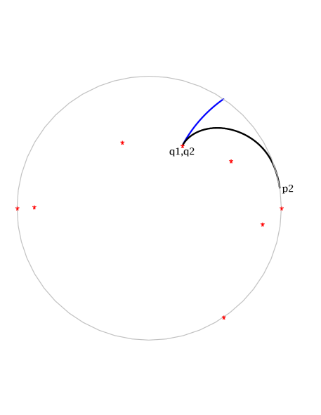
(a) $(x,y)$-projection

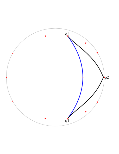
(b) $(x,t)$-projection

Figure 16. The critical points of the equations are outside $T$, in projection onto two coordinate planes.

$\Box$

Proposition 10.6.

The intersection $T\cap G_{2}^{2}T$ is empty.

Proof: We show a stronger statement, namely we show that $\partial_{\infty}C\cap G_{2}^{2}\partial_{\infty}C$ consists of precisely two points that are not in $T$. We use the same coordinates for $C$ (and $\partial_{\infty}C$) as above, write $G_{2}^{2}G_{1}^{-1}p_{0}$ and $G_{2}^{2}G_{2}^{-1}G_{3}p_{0}$ in terms of the basis given by the columns of (19), and write the equation of the intersection of $C$ with $G_{2}^{2}C$, which is simply

$$-12t_{2}t_{3}/\sqrt{5}.$$

This gives $(1,0,0)$ and $(-1,0,0)$ as the only intersection points on $\partial_{\infty}$. None of these two points is in the Dirichlet domain, a fortiori they are not in $T$. $\Box$

Martin Deraux
Institut Fourier, Université de Grenoble 1, BP 74, Saint Martin d’Hères Cedex, France
deraux@ujf-grenoble.fr

Elisha Falbel
Institut de Mathématiques, Université Pierre et Marie Curie, 4 place Jussieu, F-75252 Paris, France
falbel@math.jussieu.fr

References

- [1] A. F. Beardon. The Geometry of Discrete Groups, volume 91 of Graduate Texts in Mathematics. Springer-Verlag, New York, 1995.
- [2] N. Bergeron, E. Falbel, and A. Guilloux. Tetrahedra of flags, volume and homology of SL(3). arXiv:1101.2742.
- [3] D. Burns, Jr. and S. Shnider. Spherical hypersurfaces in complex manifolds. Invent. Math., 33(3):223–246, 1976.
- [4] M. Deraux. Deforming the -Fuchsian (4,4,4)-triangle group into a lattice. Topology, 45:989–1020, 2006.
- [5] E. Falbel. A spherical CR structure on the complement of the figure eight knot with discrete holonomy. J. Differential Geom., 79(1):69–110, 2008.
- [6] E. Falbel, P.-V. Koseleff, and F. Rouiller. Representations of fundamental groups of 3-manifolds into PGL(3,C): Exact computations in low complexity. arXiv:1307.6697.
- [7] E. Falbel and J. Wang. Branched spherical CR structures on the complement of the figure eight knot. arXiv:1304.0112.
- [8] S. Garoufalidis, M. Goerner, and C. K. Zickert. Gluing equations for PGL(n,C)-representations of 3-manifolds. arXiv:1207.6711.
- [9] W. M. Goldman. Conformally flat manifolds with nilpotent holonomy and the uniformization problem for -manifolds. Trans. Amer. Math. Soc., 278(2):573–583, 1983.
- [10] W. M. Goldman. Complex Hyperbolic Geometry. Oxford Mathematical Monographs. Oxford University Press, 1999.
- [11] B. Maskit. Kleinian groups, volume 287 of Grundlehren der Mathematischen Wissenschaften. Springer-Verlag, Berlin, 1988.
- [12] G. D. Mostow. On a remarkable class of polyhedra in complex hyperbolic space. Pacific J. Math., 86:171–276, 1980.
- [13] J. R. Parker. Complex Hyperbolic Kleinian Groups. Cambridge University Press, To appear.
- [14] M. Phillips. Dirichlet polyhedra for cyclic groups in complex hyperbolic space. Proc. Amer. Math. Soc., 115:221–228, 1992.
- [15] R. Riley. A quadratic parabolic group. Math. Proc. Cambridge Philos. Soc., 77:281–288, 1975.
- [16] D. Rolfsen. Knots and links, volume 7 of Mathematics Lecture Series. Publish or Perish Inc., Houston, TX, 1990.
- [17] R. E. Schwartz. Degenerating the complex hyperbolic ideal triangle groups. Acta Math., 186(1):105–154, 2001.
- [18] R. E. Schwartz. Real hyperbolic on the outside, complex hyperbolic on the inside. Inv. Math., 151(2):221–295, 2003.
- [19] R. E. Schwartz. Spherical CR geometry and Dehn surgery, volume 165 of Annals of Mathematics Studies. Princeton University Press, 2007.
- [20] W. P. Thurston. The Geometry and Topology of Three-Manifolds. http://library.msri.org/books/gt3m, 2002. Princeton lecture notes.