Wireless Broadcast with Physical-Layer Network Coding

Abstract

This work investigates the maximum broadcast throughput and its achievability in multi-hop wireless networks with half-duplex node constraint. We allow the use of physical-layer network coding (PNC). Although the use of PNC for unicast has been extensively studied, there has been little prior work on PNC for broadcast. Our specific results are as follows: 1) For single-source broadcast, the theoretical throughput upper bound is n/(n+1), where n is the “min vertex-cut” size of the network. 2) In general, the throughput upper bound is not always achievable. 3) For grid and many other networks, the throughput upper bound n/(n+1) is achievable. Our work can be considered as an attempt to understand the relationship between max-flow and min-cut in half-duplex broadcast networks with cycles (there has been prior work on networks with cycles, but not half-duplex broadcast networks).

I Introduction

This work investigates the maximum broadcast throughput and its achievability in multi-hop wireless networks with half-duplex node constraint. It is known that for a single-source multicast network, the maximum throughput (max-flow) is equal to the min-cut with the adoption of network coding. However, the result is for networks with full-duplex links that operate independently without mutual interference. Our work can be considered as an attempt to understand the relationship between max-flow and min-cut in networks with half-duplex nodes that may interfere with each other, such as those in wireless networks.

We allow the use of physical-layer network coding (PNC) [1]. PNC is a technique that makes possible the utilization of interfering signals. In wireless networks, when multiple transmitters transmit simultaneously, what is received at a wireless receiver is a superposition of the signals. Rather than discarding these “collided signals”, a PNC receiver transforms them to a network-coded message. Our specific results are as follows:

1. For single-source broadcast with the half-duplex node constraint and the wireless signal superposition property, the theoretical throughput upper bound is $n/(n+1)$, where $n$ is the “min vertex-cut” size of the network.

2. In general, the throughput upper bound $n/(n+1)$ is not always achievable.

3. For grid and many other networks, by adopting ($n+1$)-color partitioning and using PNC, the throughput upper bound $n/(n+1)$ is achievable.

II Related Works

In graph theory [2], the max-flow min-cut theorem specifies that the maximum throughput in a single-source unicast network is equal to the min-cut. Network coding [3] provides a solution to achieve the upper bound min-cut throughput in a single-source multicast network. Linear network coding was showed to suffice to achieve the optimum for multicast problem in [4] and [5]. A polynomial complexity algorithm to construct deterministic network codes that achieve the multicast capacity is given in [6]. Ref. [7] and [8] introduced random linear network coding and showed that it can achieve the multicast capacity with high probability. PNC, first proposed in [1], incorporates signal processing techniques to realize network coding operations at the physical layer when overlapped signals are simultaneously received from multiple transmitters. It is a foundation of our investigation here. Most existing works on PNC focus on the unicast scenario. For example, [1] studied the unicast in a two-way-relay channel, line networks and 2D grid networks; [9] and [10] study the unicast in general networks by designing distributed MAC protocols. As far as we know, there has been little, if any, prior work on broadcast with physical-layer network coding.

III System Model and Throughput Upper Bound Analysis

We consider the one-source broadcast scenario in which the packets from one source $X$ need to reach all nodes in a packet-based wireless network. Information of these packets needs to be relayed to nodes that are not within the transmission range of $X$ by other nodes.

We represent a packet-based wireless network by an undirected loopless graph $\mathcal{G}=(\mathcal{V},\mathcal{E})$, where $\mathcal{V}$ is the set of nodes and $\mathcal{E}$ is the set of links. There is a link $\{k,k^{\prime}\}\in\mathcal{E}$ between two nodes $k,k^{\prime}\in\mathcal{V}$ if and only if nodes $k$ and $k^{\prime}$ are within the direct transmission range of each other. We assume the links have equal capacity.

Packets generated and transmitted from $X$ are referred to as “native packets”. We assume equal-sized packets and synchronized time-slotted transmissions, in which all nodes are scheduled to transmit at the beginning of a time slot. A time slot is the duration of one packet. A packet $x$ is an element of $GF(2^{s})$, where $s$ is the number of bits in the packet. In other words, $x$ is a length-$s$ vector of bits.

Let $\mathcal{N}(k)$ be the set of adjacent nodes of node $k\in\mathcal{V}$. Specifically, $k^{\prime}\in\mathcal{N}(k)$ if and only if there is a link $\{k,k^{\prime}\}\in\mathcal{E}$. Each node in our network is half-duplex, i.e., it can be in either the transmission mode or the receiving mode in a given time slot, but not both. When node $k$ is in the transmission mode, it can only transmit one information stream. The same information stream reaches all neighbors of $k$, $\mathcal{N}(k)$, who are in the reception mode. When node $k$ is in the reception mode, it receives the superposed signals of its neighbors $\mathcal{N}(k)$ who are in the transmission mode. We assume that there is no interference from nodes that are two or more hops away and there is no transmission loss or error.

When a node is in the reception mode, PNC reception as defined below applies:

Definition 1 (PNC Reception).

When a node $k$ receives the superposition of multiple signals containing packets $y_{k^{\prime}}\in GF(2^{s})$ transmitted by several neighbors $k^{\prime}\in\mathcal{N}(k)$ who are in transmission mode, node $k$ maps the superposed signal to a packet $z=\bigoplus_{k^{\prime}\in\mathcal{N}(k)}y_{k^{\prime}}$. We call $z$ a PNC packet.

Readers who are interested in how PNC reception can be realized (with and without channel coding) are referred to [1, 11, 12] for details. We remark that $y_{k^{\prime}}$ transmitted by each neighbor $k^{\prime}\in\mathcal{N}(k)$ can be either a native packet or a network-coded packet. The definition of equation/packet is as follows.

Definition 2 (Equation/Packet).

An equation or a packet is expressed as

$$z=\bigoplus_{j}a_{j}x_{j}=a_{1}x_{1}\oplus a_{2}x_{2}\oplus...,$$ (1)

where $a_{j},x_{j}\in GF(2^{s})$. It is a linear combination of one or more native packets, where $a_{j}$ are the coefficients and $x_{j}$ are the native packets from $X$. Each of $a_{j}x_{j}$ in (1) is an $s$-bit vector. Similarly, the packet $z$ in (1) is also an $s$-bit vector. If there are more than one native packet combined in $z$, then we call it a network-coded packet.

In accordance with the addition and multiplication operations in $GF(2^{s})$, the addition $\oplus$ in (1) is the bit-wise XOR over $a_{j}x_{j}$ for different $j$, and the multiplication of $a_{j}$ and $x_{j}$ for each $j$ in (1) is the multiplication of their polynomial representations modulo an irreducible reducing polynomial.

The terms “packet” and “equation” will be used interchangeably in this paper. A node that has received a packet (i.e., $z$) also has acquired the associated equation, assuming the coefficients $a_{j}$ and the identities of the native packets $x_{j}$ (i.e., the indexes of the native packets) are known. Such index information can be encoded into the packet header. Conceptually, a node will be able to decode the $D$ native packets broadcast by $X$ if it has $D$ linearly independent equations (native or network-coded packets) which contains the $D$ native packets in their summands.

With reference to Definition 1 and Definition 2, for a node $k$, suppose that a subset of neighbors $\mathcal{N}^{\prime}(k)\subseteq\mathcal{N}(k)$ transmit simultaneously, and neighbor $k^{\prime}\in\mathcal{N}^{\prime}(k)$ transmits $y_{k^{\prime}}=\bigoplus_{j_{k^{\prime}}}a_{j_{k^{\prime}}}x_{j_{k^{\prime}}}$. Then, PNC reception allows node $k$ to obtain the following equation.

$$z=\bigoplus_{k^{\prime}\in\mathcal{N}^{\prime}(k)}y_{k^{\prime}}=\bigoplus_{k^{\prime}\in\mathcal{N}^{\prime}(k)}\left(\bigoplus_{j_{k^{\prime}}}a_{j_{k^{\prime}}}x_{j_{k^{\prime}}}\right)$$ (2)

Note that node $k^{\prime}$ that transmits $y_{k^{\prime}}=\bigoplus_{j_{k^{\prime}}}a_{j_{k^{\prime}}}x_{j_{k^{\prime}}}$ may perform upper-layer network coding to obtain $y_{k^{\prime}}=\bigoplus_{j_{k^{\prime}}}a_{j_{k^{\prime}}}x_{j_{k^{\prime}}}$ from the data that it has received so far. That is, in (2) above, $y_{k^{\prime}}$ is a packet (possibly native or network-coded) generated by the upper layer of a transmitting node; whereas $z$ is a physical-layer network-coded packet generated at the receiving node based on the simultaneous signals from multiple transmitting source. In this paper, we will be using PNC as well as upper-layer network coding to enable efficient broadcasting.

Definition 3 (Trivial Network).

Consider a network $\mathcal{G}=(\mathcal{V},\mathcal{E})$. If all nodes in the network are neighbors of $X$ (i.e., $\mathcal{N}(X)=\mathcal{V}\backslash\{X\}$), then the network is called a trivial network.

In a trivial network, all non-source nodes can receive directly from $X$. Relaying information from a node to the other is thus unnecessary. The optimal strategy is for $X$ to transmit all the time and all other nodes to receive all the time, and the normalized broadcast throughput is 1. In this paper, we are only interested in non-trivial networks.

Consider a cut $C=(\mathcal{V}_{1},\mathcal{V}_{2})$ in a network $\mathcal{G}=(\mathcal{V},\mathcal{E})$ that partitions the nodes $\mathcal{V}$ in into two subsets $\mathcal{V}_{1}$and $\mathcal{V}_{2}$. Let $\mathcal{V}_{1}$ be the subset that contains $X$. Let $\mathcal{V}_{1}^{\prime}\subseteq\mathcal{V}_{1}$ be nodes in $\mathcal{V}_{1}$ that has neighbors in $\mathcal{V}_{2}$, and $\mathcal{V}_{2}^{\prime}\subseteq\mathcal{V}_{2}$ to be nodes in $\mathcal{V}_{2}$ that has neighbors in $\mathcal{V}_{1}$. That is, the nodes in $\mathcal{V}_{1}\backslash\mathcal{V}_{1}^{\prime}$ and the nodes in $\mathcal{V}_{2}\backslash\mathcal{V}_{2}^{\prime}$ are not connected. The information from $X$ has to go through some nodes in $\mathcal{V}_{1}^{\prime}$ in order to reach nodes in $\mathcal{V}_{2}$.

Figure 1: Partitioning with a qualified cut

Definition 4 (Vertex-Cut Size).

Consider a cut $C$. Let $\mathcal{V}_{1},\mathcal{V}_{2},\mathcal{V}_{1}^{\prime}$ and $\mathcal{V}_{2}^{\prime}$ be defined as above. The vertex-cut size of $C$ is $|\mathcal{V}_{1}^{\prime}|$.

Note the difference between the definition of the traditional cut size and the above vertex-cut size. The traditional cut size is defined to be the number of edges from nodes in $\mathcal{V}_{1}^{\prime}$ to nodes in $\mathcal{V}_{2}^{\prime}$. The motivation for the above vertex-cut size is due to the wireless node constraint we assume: specifically, a node cannot transmit different information on different links incident to it; when it transmits, it broadcasts the same information on all these links. Thus, the vertex-cut size better characterizes the maximum flow that can go from $\mathcal{V}_{1}$ to $\mathcal{V}_{2}$.

Definition 5 (Qualified Cut).

Consider a cut $C=(\mathcal{V}_{1},\mathcal{V}_{2})$. Let $\mathcal{V}_{1},\mathcal{V}_{2},\mathcal{V}_{1}^{\prime}$ and $\mathcal{V}_{2}^{\prime}$ be defined as above. $C$ is said to be a qualified cut if and only if $X\notin\mathcal{V}_{1}^{\prime}$.

Fig. 1 shows the partitioning with a qualified cut. A qualified cut ensures the adjacent nodes of $X$ are in the same sub-network, $\mathcal{V}_{1}$, as $X$. A qualified cut does not exist in a trivial network, and can always be found in a non-trivial network. Intuitively, the broadcast throughput from $X$ to all other nodes is limited by the need to relay information to nodes that are not direct neighbors of source $X$. Thus, the throughput limit should be characterized by the qualified cut in that it characterizes the “relay capacity” to nodes that are two or more hops away from $X$.

Recall that we are interested in the problem of source $X$ broadcasting $D$ native packets to all other nodes in the network for large $D$. Let $W_{D}$ be the number of time slots needed before all nodes acquire all the $D$ native packets. The $D$ native packets can be obtained if a node has received $D$ linearly independent equations relating the $D$ native packets.

Definition 6 (Throughput).

The broadcast throughput $\rho$ of source $X$ is $\lim_{D\rightarrow\infty}D/W_{D}$.

Each qualified cut has an associated vertex-cut size. The qualified cuts with the minimum vertex-cut size in the network are called the minimum qualified cuts. The following theorem gives an upper bound on the achievable broadcast throughput:

Theorem 1.

Consider a non-trivial network $\mathcal{G}$ whose minimum qualified cuts have vertex-cut size $n$. Then $\rho\leq n/(n+1)$.

Proof:

With respect to Definition 5, let $C$ be a minimum qualified cut with vertex-cut size $n$. Suppose the $D$ packets to be broadcast by $X$ are $\{x(0),...,x(D-1)\}$. There are two ways to deliver information related to these $D$ native packets from nodes in $\mathcal{V}_{1}^{\prime}$ to nodes in $\mathcal{V}_{2}^{\prime}$:
1) deliver the information directly in the original form of the $D$ native packets; or
2) deliver at least $D$ linearly independent equations (native or network-coded packets) with $x(0),...,x(D-1)$ as unknowns.
Either way, there must be at least $D$ transmissions (taking up $D$ time slots) from nodes in $\mathcal{V}_{1}^{\prime}$ to nodes in $\mathcal{V}_{2}^{\prime}$.

We label the nodes in $\mathcal{V}_{1}^{\prime}$ by $1,2,...,n$ (see Fig. 1). Let $T_{1},T_{2},...,T_{n}$ be the numbers of packets transmitted by nodes $1,2,...,n$, respectively, by the end of $W_{D}$ time slots. Let $R_{1},R_{2},...,R_{n}$ be the numbers of packets received by nodes $1,2,...,n$, respectively, by the end of $W_{D}$ time slots. Since a node is either in the transmission mode or in the receiving mode in each of the $W_{D}$ time slots, we have

$$W_{D}=T_{i}+R_{i}\mbox{ for all nodes }i,1\leq i\leq n.$$ (3)

Furthermore, since each node $i,1\leq i\leq n$, must have received at least $D$ linearly independent equations to decode the $D$ native packets, we must have

$$R_{i}\geq D\mbox{ for all nodes }i,1\leq i\leq n.$$ (4)

In addition, at least $D$ linearly independent equations must be delivered to nodes in $\mathcal{V}{}_{2}^{\prime}$ from nodes in $\mathcal{V}{}_{1}^{\prime}$, meaning

$$T_{1}+T_{2}+...+T_{n}\geq D.$$ (5)

Thus, the network throughput is

$$\rho=\lim_{D\rightarrow\infty}\frac{D}{W_{D}}=\lim_{D\rightarrow\infty}\frac{D}{T_{i}+R_{i}}\;\enskip\forall 1\leq i\leq n.$$ (6)

Thus,

$$\rho\leq\min_{1\leq i\leq n}\lim_{D\rightarrow\infty}\frac{D}{T_{i}+D}.$$ (7)

Note that $T_{1},T_{2},...,T_{n}$ and $R_{1},R_{2},...,R_{n}$ (i.e., how many times each node transmits and how many times each node receives) depend on the detailed scheduling and relaying scheme. Here, we are interested in an upper bound that is valid for all schemes, including the optimal scheduling scheme. Thus, we solve the following optimization problem:

$$\max\min_{1\leq i\leq n}\lim_{D\rightarrow\infty}\frac{D}{T_{i}+D}$$ (8)

such that $T_{1}+T_{2}+...+T_{n}\geq D$. As $D\rightarrow\infty$, the solution to the above problem is given by

$$T_{i}=\frac{D}{n},\forall 1\leq i\leq n.$$ (9)

An upper bound of $\rho$ is therefore given by

$$\rho\leq\lim_{D\rightarrow\infty}\frac{D}{\frac{D}{n}+D}=\frac{n}{n+1}$$ (10)

∎

The upper bound of broadcast throughput is not always achievable. For example, the minimum qualified cut in the network shown in Fig. 2 has vertex-cut size 2. However, a throughput of $2/3$ cannot be achieved. The reader is referred to Appendix -A for details.

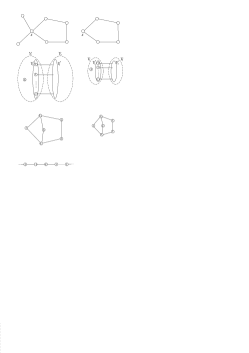
Figure 2: Example of a network whose broadcast throughput cannot reach the upper bound $n/(n+1)$

Although not always achievable in general, the throughput upper bound $n/(n+1)$ is achievable in many networks, including line, ring, chord ring, and grid networks. Section IV shows the achievability for line, ring, and chord ring. Section VI shows its achievability in grid networks.

IV Broadcast Scheme for Line, Ring & Chord Ring Networks

Line Networks

Fig. 3 gives an example of a PNC broadcast scheme in a line network with five nodes. By Theorem 1, the broadcast throughput upper bound of this network is $1/2$. The following describes a scheduling scheme that can achieve this upper bound. In line networks, the nodes only need to transmit native packets without doing higher layer network coding. However, in other cases to be presented later, higher layer network coding may be performed.

At $ts=0$, source $X$ transmits $x(0)$ to its neighbor node, i.e., node $1$.

At $ts=1$, node $1$ broadcast $x(0)$ to its neighbors, i.e., $X$ and node $2$. As $X$ is the source, it simply discards the received packet.

At $ts=2$, $X$ and node $2$ transmit $x(1)$ and $x(0)$, respectively, to their neighbors. Node $1$ receives a superposition of $x(0)$ and $x(1)$ and maps it to $x(0)\oplus x(1)$ through PNC. As node $1$ already has $x(0)$, it can derive $x(1)$ from $x(0)\oplus x(1)$.

At $ts=3$, nodes $1$ and $3$ broadcast $x(1)$ and $x(0)$, respectively, to their neighbors. Node $2$ receives a superposition of $x(0)$ and $x(1)$, maps it to $x(0)\oplus x(1)$ and derives $x(1)$ with the knowledge of $x(0)$. Node $4$ receives $x(0)$.

At $ts=4$, $X$, node $2$ and node $4$ transmit $x(2)$, $x(1)$ and $x(0)$, respectively, to their neighbors. Similar to $ts=2$, node $1$ derives $x(2)$ from $x(1)\oplus x(2)$ with the knowledge of $x(1)$; node $3$ derives $x(1)$ from $x(0)\oplus x(1)$ with the knowledge of $x(0)$.

For $ts\geq 5$, the pattern continues.

Overall, over the long term, the throughput of $X$ is $1/2$, as it delivers one new packet to all other nodes in the network in every two time slots. The pattern also works if there are nodes to the left of $X$.

For comparison, an example of traditional store-and-forward broadcast in the same line network is showed in Fig. 4. The throughput of $X$ in this case is $1/3$, as it delivers one new packet to all other nodes in the network in every three time slots.

Note that for one-source broadcast with PNC in line networks, the transmitters only need to transmit native packets to achieve the optimal performance, although the received packets under PNC reception can be network-coded. For one-source broadcast in the ring networks, the transmitters will need to transmit network-coded packets. The following will treat this case.

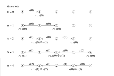
Figure 3: Example of PNC broadcast in a line network with five nodes. “$r$” indicates “receive”.

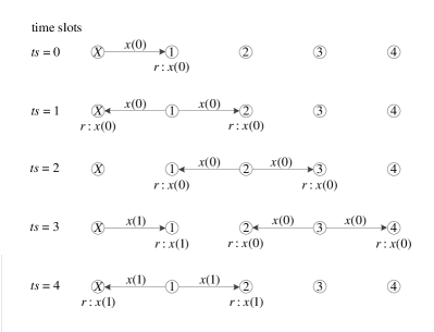
Figure 4: Example of traditional store-and-forward broadcast in a line network with five nodes.

Ring Networks

Fig. 5 shows a ring network with six nodes. By Theorem 1, its broadcast throughput upper bound with PNC is $2/3$. Table I describes a scheme that can achieve the upper bound. Node $3$ needs to perform higher layer network coding before transmissions. Note that we denote the sequence of native packets to be broadcast by $X$ by $\{x_{0}(t)\}_{t=0,1,2,..}$ and $\{x_{1}(t)\}_{t=0,1,2,..}$. We define a round $t,t=0,1,2,...$ to be a set of three time slots $\{3t,3t+1,3t+2\}$.

Note that in time slot 9, node 3 transmits $x_{0}(0)\oplus x_{1}(0)$. Upon receiving $x_{0}(0)\oplus x_{1}(0)$, node 2 can decode $x_{1}(0)$ because it already has $x_{0}(0)$; node 4 can decode $x_{0}(0)$ because it has $x_{1}(0)$. From round 3 onwards, every non-source node receives sufficient information for it to derive two new native packets in each round. Thus, the throughput is $2/3$.

TABLE I: PNC broadcast schedule for the ring network in Fig. 5. “s”, “r” and “d” indicate “send”, “receive” and “derive”, respectively.

t	ts	Node $X$	Node 1	Node 2	Node 3	Node 4	Node 5
0	0	s:$x_{0}(0)$	r:$x_{0}(0)$	-	-	-	r:$x_{0}(0)$
	1	s:$x_{1}(0)$	r:$x_{1}(0)$	-	-	-	r:$x_{1}(0)$
	2	s:$x_{0}(0)$ $\oplus x_{1}(0)$	-	-	-	-	-
1	3	s:$x_{0}(1)$	r:$x_{0}(1)$	-	-	-	r:$x_{0}(1)$
	4	s:$x_{1}(1)$	s:$x_{0}(0)$	r:$x_{0}(0)$	-	-	r:$x_{1}(1)$
	5	s:$x_{0}(1)$ $\oplus x_{1}(1)$	r:$x_{0}(1)$ $\oplus x_{1}(1)$ d:$x_{1}(1)$	-	-	r:$x_{1}(0)$	s:$x_{1}(0)$
2	6	s:$x_{0}(2)$	r:$x_{0}(2)$	-	-	-	r:$x_{0}(2)$
	7	s:$x_{1}(2)$	s:$x_{0}(1)$	r:$x_{0}(1)$	r:$x_{1}(0)$	s:$x_{1}(0)$	r:$x_{1}(2)$ $\oplus x_{1}(0)$ d:$x_{1}(2)$
	8	s:$x_{0}(2)$ $\oplus x_{1}(2)$	r:$x_{0}(2)$ $\oplus x_{1}(2)$ $\oplus x_{0}(0)$ d:$x_{1}(2)$	s:$x_{0}(0)$	r:$x_{0}(0)$	r:$x_{1}(1)$	s:$x_{1}(1)$
3	9	s:$x_{0}(3)$	r:$x_{0}(3)$	r:$x_{0}(0)$ $\oplus x_{1}(0)$ d:$x_{1}(0)$	s:$x_{0}(0)$ $\oplus x_{1}(0)$	r:$x_{0}(0)$ $\oplus x_{1}(0)$ d:$x_{0}(0)$	r:$x_{0}(3)$
	10	s:$x_{1}(3)$	s:$x_{0}(2)$	r:$x_{0}(2)$	r:$x_{1}(1)$	s:$x_{1}(1)$	r:$x_{1}(3)$ $\oplus x_{1}(1)$ d:$x_{1}(3)$
	11	s:$x_{0}(3)$ $\oplus x_{1}(3)$	r:$x_{0}(3)$ $\oplus x_{1}(3)$ $\oplus x_{0}(1)$ d:$x_{1}(3)$	s:$x_{0}(1)$	r:$x_{0}(1)$	r:$x_{1}(2)$	s:$x_{1}(2)$
4	12	s:$x_{0}(4)$	r:$x_{0}(4)$	r:$x_{0}(1)$ $\oplus x_{1}(1)$ d:$x_{1}(1)$	s:$x_{0}(1)$ $\oplus x_{1}(1)$	r:$x_{0}(1)$ $\oplus x_{1}(1)$ d:$x_{0}(1)$	r:$x_{0}(4)$
	13	s:$x_{1}(4)$	s:$x_{0}(3)$	r:$x_{0}(3)$	r:$x_{0}(0)$ $\oplus x_{1}(2)$ d:$x_{1}(2)$	s:$x_{0}(0)$ $\oplus x_{1}(2)$	r:$x_{1}(4)$ $\oplus x_{0}(0)$ $\oplus x_{1}(0)$ $\oplus x_{1}(2)$ d:$x_{1}(4)$
	14	s:$x_{0}(4)$ $\oplus x_{1}(4)$	r:$x_{0}(4)$ $\oplus x_{1}(4)$ $\oplus x_{0}(2)$ $\oplus x_{1}(0)$ d:$x_{1}(4)$	s:$x_{0}(2)$ $\oplus x_{1}(0)$	r:$x_{0}(2)$ $\oplus x_{1}(0)$ d:$x_{0}(2)$	r:$x_{1}(3)$	s:$x_{1}(3)$

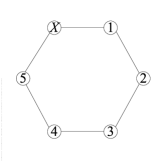
Figure 5: A ring network

Chord Ring Networks

Fig. 6 shows a chord ring network with six nodes. By Theorem 1, its broadcast throughput upper bound is $4/5$. A transmission scheme for this network is described in Appendix -B.

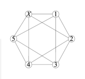
Figure 6: A chord ring network

V Color-based Scheduling

Color-based scheduling can be used to achieve the throughput upper bound in Theorem 1 in some networks.

Definition 7 (Vertex Coloring).

Consider a graph $\mathcal{G}=(\mathcal{V},\mathcal{E})$. Let $\mathcal{C}$ be a set of colors. A vertex coloring scheme $f:\mathcal{V}\to\mathcal{C}$ assigns to each vertex $v\in\mathcal{V}$ a color $c\in\mathcal{C}$.

Definition 8 (Colored Graph).

Consider a graph $\mathcal{G}=(\mathcal{V},\mathcal{E})$ and a particular vertex coloring scheme $f:\mathcal{V}\to\mathcal{C}$ for it. The resulting colored graph is $\mathcal{G}_{f}=(\mathcal{V},\mathcal{E}_{f},f)$, where $\mathcal{E}_{f}\subseteq\mathcal{E}$ such that an edge $e=\{k,k^{\prime}\}\in\mathcal{E}$ is also an element in $\mathcal{E}_{f}$ if and only if $f(k)\neq f(k^{\prime})$. In other words, besides assigning colors to the vertices, we also remove edges between vertices of like color to obtain the colored graph $\mathcal{G}_{f}$.

Definition 9 (Color Group).

Consider a graph $\mathcal{G}=(\mathcal{V},\mathcal{E})$ and an associated colored graph $\mathcal{G}_{f}=(\mathcal{V},\mathcal{E}_{f},f)$. Consider a qualified cut $C$ on the colored graph. The definitions of $\mathcal{V}_{1}$, $\mathcal{V}_{2}$, $\mathcal{V}_{1}^{\prime}$, $\mathcal{V}_{2}^{\prime}$ are the same as in Definition 4 and Fig. 1 (note that given the same $\mathcal{V}_{1}$ and $\mathcal{V}_{2}$ in the qualified cut, the $\mathcal{V}_{1}^{\prime}$ and $\mathcal{V}_{2}^{\prime}$ in $\mathcal{G}_{f}$ and the $\mathcal{V}_{1}^{\prime}$ and $\mathcal{V}_{2}^{\prime}$ in $\mathcal{G}$ may be different because $\mathcal{E}_{f}\subseteq\mathcal{E}$). We divide the vertices in $\mathcal{V}_{1}^{\prime}$ into different sets according to the vertex color. Each of these vertex sets is called a color group. A color-$c$ group is a color group wherein the vertices have color $c\in\mathcal{C}$.

Definition 10 (Color-group Cut Size).

With the same definitions of $\mathcal{G}$, $\mathcal{G}_{f}$, $C$, $\mathcal{V}_{1}$, $\mathcal{V}_{2}$, $\mathcal{V}_{1}^{\prime}$, $\mathcal{V}_{2}^{\prime}$ as above. Let $\mathcal{U}_{c}$ be a color-$c$ group in $\mathcal{V}_{1}^{\prime}$. We form a matrix where rows represent vertices in $\mathcal{U}_{c}$, and columns represent vertices in $\mathcal{V}_{2}^{\prime}$. Consider $u\in\mathcal{U}_{c},v\in\mathcal{V}_{2}^{\prime}$. The $(u,v)$-th entry is 1 if and only if $(u,v)\in\mathcal{E}$; it is 0 otherwise. The color-group cut size of $\mathcal{U}_{c}$ is the rank of this matrix.

Definition 11 (Color-cut Size).

With the same definitions of $\mathcal{G}$, $\mathcal{G}_{f}$, $C$, $\mathcal{V}_{1}$, $\mathcal{V}_{2}$, $\mathcal{V}_{1}^{\prime}$, $\mathcal{V}_{2}^{\prime}$, $\mathcal{U}_{c}$ as above. Let $G_{c}$ be the color-group cut size of $\mathcal{U}_{c}$. The color-cut size of $C$ is the sum of the color-group cut size of all color groups, $\sum_{c\in\mathcal{C}}G_{c}$.

For illustration, Fig. 7 shows the partitioning of a colored graph with a qualified cut. There are three colors $\{0,1,2\}$. The color-0 group has a color-group cut size of 2, as

$$\mbox{rank}\left[\begin{array}[]{cccccc}1&1&1&0&0&0\\ 1&0&1&0&0&0\\ 0&1&0&0&0&0\end{array}\right]=2.$$

The color-1 group has a color-group cut size of 3, as

$$\mbox{rank}\left[\begin{array}[]{cccccc}0&0&1&1&0&0\\ 0&0&0&1&1&0\\ 0&0&0&0&1&0\end{array}\right]=3.$$

The color-2 group has a color-group cut size of 1, as

$$\mbox{rank}\left[\begin{array}[]{cccccc}0&0&0&0&0&1\\ 0&0&0&0&0&1\end{array}\right]=1.$$

Thus, the color-cut size is $2+3+1=6$.

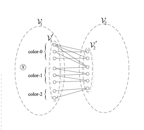
Figure 7: A qualified cut with color-cut size 6

Definition 12 (Color-based Scheduling).

Consider a network and an associated colored graph. A color-based scheduling is a schedule such that nodes with the same color transmit in the same time slots, and nodes with different colors transmit in different time slots.

With a color-based scheduling, the color-group cut size represents the maximum number of linearly independent equations the color group can deliver across the cut in a time slot.

Theorem 2.

Consider a non-trivial network $\mathcal{G}$ and an associated colored graph $\mathcal{G}_{f}$. Suppose that the minimum color-cut size among all qualified cuts is $n_{f}$. Then $\rho\leq n_{f}/(n_{f}+1)$ with any color-based scheduling.

Proof:

With respect to Definition 5, let $C$ be a qualified cut of $\mathcal{G}_{f}$ with minimum color-cut size $n_{f}$. The number of distinct colors in $\mathcal{V}_{1}^{\prime}$ is $|f(\mathcal{V}_{1}^{\prime})|$. We divide the nodes in $\mathcal{V}_{1}^{\prime}$ into $|f(\mathcal{V}_{1}^{\prime})|$ color groups. Let $G_{c}$ be the color-group cut size of color-$c$ group, $c\in f(\mathcal{V}_{1}^{\prime})\subseteq\mathcal{C}$. We have

$$n_{f}=\sum_{c\in|f(\mathcal{V}_{1}^{\prime})|}G_{c}.$$ (11)

Let $T_{c}$ be the number of time slots during which nodes in color-$c$ group transmits within the $W_{D}$ time slots (see Definition 6 for the definition of $W_{D}$); let $R_{c}$ be the number of time slots during which nodes in color-$c$ group receives within the $W_{D}$ time slots. We have

$$W_{D}=T_{c}+R_{c}\;\enskip\forall c\in f(\mathcal{V}_{1}^{\prime}).$$ (12)

Furthermore, since each node must receive at least $D$ linearly independent equations to decode the $D$ native packets, we must have

$$R_{c}\geq D\;\enskip\forall c\in f(\mathcal{V}_{1}^{\prime}).$$ (13)

In addition, at least $D$ linearly independent equations must be delivered to nodes in $\mathcal{V}{}_{2}^{\prime}$ from nodes in $\mathcal{V}{}_{1}^{\prime}$, meaning

$$\sum_{c\in f(\mathcal{V}_{1}^{\prime})}T_{c}G_{c}\geq D.$$ (14)

The LHS of (14) is from the fact that a color group can deliver at most $G_{c}$ linearly independent equations across the cut per time slot. Notice the difference between (14) and (5). Theorem 1 gives the general upper bound. Theorem 2 here considers the upper bound assuming the adoption of color-based scheduling. Since in color-based scheduling nodes of the same color transmit in the same time slots, the number of equations crossing from $\mathcal{V}_{1}^{\prime}$ to $\mathcal{V}_{2}^{\prime}$ in the colored graph is $\sum_{c\in f(\mathcal{V}_{1}^{\prime})}T_{c}G_{c}$, of which $D$ must be linearly independent. The network throughput is

$$\rho=\lim_{D\rightarrow\infty}\frac{D}{W_{D}}=\lim_{D\rightarrow\infty}\frac{D}{T_{c}+R_{c}}\;\enskip\forall c\in f(\mathcal{V}_{1}^{\prime}).$$ (15)

Thus,

$$\rho\leq\min_{c\in f(\mathcal{V}_{1}^{\prime})}\lim_{D\rightarrow\infty}\frac{D}{T_{c}+D}.$$ (16)

To obtain an upper bound that is valid for all coloring schemes, we solve the following optimization problem

$$\max\min_{c\in f(\mathcal{V}_{1}^{\prime})}\lim_{D\rightarrow\infty}\frac{D}{T_{c}+D}$$ (17)

such that $\sum_{c\in f(\mathcal{V}_{1}^{\prime})}T_{c}G_{c}\geq D$. The minimum $\lim_{D\rightarrow\infty}D/(T_{c}+D)$ is obtained at the maximum $T_{c}$; therefore, to maximize $\min_{c\in f(\mathcal{V}_{1}^{\prime})}\lim_{D\rightarrow\infty}D/(T_{c}+D)$, we need to minimize $\max T_{c}$. Suppose that $T_{c_{1}}=\max T_{c}$ for some $c_{1}\in f(\mathcal{V}_{1}^{\prime})$. If there exists $T_{c_{2}}$, $c_{2}\in f(\mathcal{V}_{1}^{\prime})$, such that

$$T_{c_{1}}>T_{c_{2}}$$ (18)

then $T_{c_{1}}=\max T_{c}$ can be made smaller by allocating part of the time slots from $T_{c_{1}}$ to $T_{c_{2}}$. As $D\rightarrow\infty$, we require that

$$T_{c_{1}}=T_{c_{2}}=...=\max T_{c}\;\enskip c_{1},c_{2},...\in f(\mathcal{V}_{1}^{\prime})$$ (19)

in order that $\max T_{c}$ is minimized. Let $T$ be such $\max T_{c}$. The solution to the above problem is given by

$$\sum_{c\in f(\mathcal{V}_{1}^{\prime})}T_{c}G_{c}\geq D\Rightarrow T\sum_{c\in f(\mathcal{V}_{1}^{\prime})}G_{c}\geq D\Rightarrow Tn_{f}\geq D$$ (20)

$$\Rightarrow T\geq\frac{D}{n_{f}}$$ (21)

An upper bound of $\rho$ is therefore given by

$$\rho\leq\lim_{D\rightarrow\infty}\frac{D}{\frac{D}{n_{f}}+D}=\frac{n_{f}}{n_{f}+1}$$ (22)

∎

With Theorems 1 and 2, we now have

$$\rho\leq\min(\frac{n}{n+1},\frac{n_{f}}{n_{f}+1}),$$ (23)

where $n$ is the minimum qualified cut in $\mathcal{G}$ and $n_{f}$ is the minimum color-cut size among all qualified cuts in $\mathcal{G}_{f}$. In general, it is obvious that $n\geq n_{f}$. Thus, if color-based scheduling is used, $n_{f}/(n_{f}+1)$ is a tighter bound than $n/(n+1)$, which is obvious since colored-based scheduling is only a subset of possible scheduling schemes. In order that the general upper bound $n/(n+1)$ can be achieved with color-based scheduling, we must color $\mathcal{G}$ in such a way that the resulting colored graph $\mathcal{G}_{f}$ has $n_{f}=n$. We will show in Section VI that a specific color-based scheduling scheme can be constructed for grid networks to achieve the broadcast throughput upper bound $n/(n+1)=2/3$. In this scheme, the associated colored graph $\mathcal{G}_{f}$ for the grid has $n_{f}=n=2$.

VI Broadcast Scheme for Grid Networks

VI-A Overview

In grid networks, $n=2$ and thus $\rho\leq n/(n+1)=2/3$. The goal of this section is to prove that the throughput upper bound is achievable. As the proof is quite involved, requiring the introduction of a number of new concepts, we first give an overview of our approach here.

Our proof is a constructive proof. Specifically, we adopt a color-based scheduling scheme with three colors.

In Section VI-B, we first review the concept of an embedded Hamiltonian cycle within a grid network. The nodes in the grid are colored according to their position in the embedded Hamiltonian cycle, with the three colors assigned to successive nodes in a repetitive manner, as in color 0, color 1, color 2, color 0, color 1, color 2, and so on. In the resulting colored graph, each node is guaranteed to have two neighbors of two different colors. That is, the node and these two neighbors cover the three available colors. Note that if the neighbors of a node were all of the same color, then according to Theorem 2, the throughput upper bound would be $1/2$ (because $n_{f}=1$), and our target of achieving throughput of $2/3$ would not be possible.In that light, the Hamiltonian-cycle coloring scheme here is designed to ensure a necessary condition is not violated.

In color-based scheduling, nodes with the same color transmit in the same time slots. In Section VI-C, we specify when a node should transmit and what it should transmit during its transmission time slots. The key concept is that we divide the time slots into rounds, with each round consisting of three time slots corresponding to the three colors. Thus, each node gets to transmit once in each round in the time slot associated with its color. Also, each node receives in two time slots in each round. If the information received during its reception time slots are independent, then throughput of $2/3$ is possible. In our scheme, the information transmitted by a node in a round is basically the sum of the two packets it received in the last round multiplied by a coefficient. We refer to this coefficient as the transmit coefficient.

The transmit coefficients used by the nodes in the network determine whether each node can receive two independent linear equations in each round. In Section VI-D, we describe a scheme in which random transmit coefficients are used by the node. Specifically, the transmit coefficient used by a node is drawn from $GF(2^{s})\backslash\{0\}$ uniform-randomly in each round. This is an i.i.d. time-varying transmit coefficient assignment scheme, since the transmit coefficient of a node changes from round to round. We choose to use this scheme mainly to simplify the proof. We argue that provided the field size $2^{s}$ is large, with high probability the linear equations received in all time slots are linearly independent. Hence, throughput of $2/3$ is achievable.

VI-B Coloring of networks by constructing Hamiltonian cycles

A Hamiltonian cycle is a path that visits each node in a graph exactly once and ends at its starting point. First, for any $M\times N$ grid graph with at least one of $M,N$ being even, there is a Hamiltonian cycle in the graph [2]. For example, we can construct a comb-shaped Hamiltonian cycle as shown in Fig. 8a. Starting from a neighbor of $X$ on the cycle, we number along the path by 1-2-3-…-($MN$-1). Depicted in Fig. 8b is an example of this numbering scheme in a $6\times 5$ grid with $X=(1,1)$.

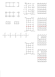
(a) A Hamiltonian cycle in an $M\times N$ network ($M$ is even).

(b) Numbering of nodes in a $6\times 5$ network after renumbering.

Figure 8: $M\times N$ networks with at least one of $M,N$ being even

Next, if $M$ and $N$ are both odd, then it is not possible to construct a Hamiltonian cycle in the grid [2]. Instead, we construct a pseudo Hamiltonian cycle called the “Split-Merge Hamiltonian cycle”, as illustrated in Fig. 9a and 9b. As shown in Fig. 9b, after visiting node 5, the visits split into two paths. Nodes 6 and 6* are visited in parallel next; node 7 and 7* after that; and then node 8 and 8*; finally the parallel visits merge back to node 9. By splitting and merging as such, a result is the insertion of a new row (as indicated red in Fig. 9a and 9b) into an $(M-1)\times N$ network which already has a Hamiltonian cycle constructed (because $M-1$ is even, we can construct such a cycle).

(a) A Hamiltonian cycle in an $M\times N$ network ($M$ and $N$ are both odd). Part of the cycle contains two parallel paths.

(b) Numbering of nodes in a $7\times 5$ network.

Figure 9: $M\times N$ networks with both $M,N$ being odd

Hamiltonian Node Coloring: Now that we have a node numbering scheme for all grid networks, we partition the non-source nodes into nodes of three distinct colors $c\in\{0,1,2\}$ with a vertex coloring scheme given by $f(k)=k\bmod 3$. That is, we assign node $k$ the color $c=k\bmod 3$. We also let $f(k^{*}):=f(k)$, i.e., let the node $k^{*}$ in the split paths have the same color as node $k$.

Fig. 10 shows the colored graphs produced after applying the Hamiltonian coloring to networks in Fig. 8b and Fig. 9b. Once we have colored the nodes, we then remove links between nodes of the same color. The result is a colored graph embedded in the original grid graph. The minimum qualified cut size is $n=2$ in grid networks. One can verify that the minimum color-cut size is $n_{f}=2$ in grid networks with the coloring scheme above. Therefore by Theorem 2 the broadcast throughput upper bound is still $2/3$, thus is not decreased by the Hamiltonian coloring scheme.

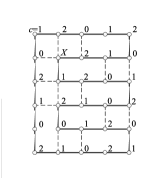
(a) $6\times 5$

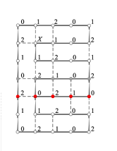
(b) $7\times 5$

Figure 10: Colored graphs of $6\times 5$ and $7\times 5$ grid networks.

The motivation for the above Hamiltonian coloring is as follows. A node $k$ that is two or more hops away from $X$ can only receive the broadcast information from $X$ through its neighbors $\mathcal{N}(k)$. In our time-slotted scheme, the nodes with the same color transmit at the same time. The Hamiltonian coloring scheme ensures that each node $k$ has at least two neighbors assigned with the two colors different from the color of node $k$. These two other colors correspond to the time slots in which node $k$ receives. Thus, each node $k$ receives in at least two time slots out of every three time slots. Section VI-C specifies this transmission scheme more exactly.

VI-C Ternary transmission schedule

Our basic idea is to let nodes with color $c$ transmit in time slots $3t+c,t=0,1,2...$ As a consequence, every node transmits once and receives twice in every round $t,t=0,1,2,...$, a set of three time slots $\{3t,3t+1,3t+2\}$.

If we could ensure that in each round, every node receives two packets that contain new information, then the broadcast throughput would be $2/3$, which is the upper bound given by Theorem 1. Toward that end, we propose a schedule with the following four rules (also summarized in Table II):

TABLE II: Ternary transmission schedule

ts	Node $X$	$X_{0}$ (Node 1)	$X_{1}$ (Node $MN-1$)	Color-0 nodes	Color-1 nodes	Color-2 nodes
$3t$	$x_{0}(t)$	-	$x_{1}(t-1)$ if $(MN-1)\bmod 3=0$; nothing otherwise	$\alpha_{k}(z_{0}^{k}(t)\oplus z_{1}^{k}(t))$	-	-
$3t+1$	$x_{1}(t)$	$x_{0}(t-1)$	$x_{1}(t-1)$ if $(MN-1)\bmod 3=1$; nothing otherwise	-	$\alpha_{k}(z_{0}^{k}(t)\oplus z_{1}^{k}(t))$	-
$3t+2$	$x_{0}(t)\oplus x_{1}(t)$	-	$x_{1}(t-1)$ if $(MN-1)\bmod 3=2$; nothing otherwise	-	-	$\alpha_{k}(z_{0}^{k}(t)\oplus z_{1}^{k}(t))$

Rule 1) Transmissions by source $\bm{X}$: Let the sequence of native packets to be broadcast by $X$ be $\{x_{0}(t)\}_{t=0,1,2,..}$ and $\{x_{1}(t)\}_{t=0,1,2,..}$. In time slot $3t$, $X$ transmits $x_{0}(t)$; in time slot $3t+1$, $X$ transmits $x_{1}(t)$; in time slot $3t+2$, $X$ transmits $x_{0}(t)\oplus x_{1}(t)$.

Rule 2) Transmissions by nodes not adjacent to $\bm{X}$: In time slot $3t+c,c\in\{0,1,2\}$, node $k$, $k\notin\mathcal{N}(X)$, with color $c$ transmits

$$y^{k}(t)=\alpha_{k}(z_{0}^{k}(t)\oplus z_{1}^{k}(t)),$$

where $\alpha_{k}\in GF(2^{s})\backslash\{0\}$ is a transmit coefficient, and

$$z_{0}^{k}(t)=r_{0}^{k}(t-1)$$

$$z_{1}^{k}(t)=r_{1}^{k}(t-1)$$

In the above, $r_{0}^{k}(t-1),r_{1}^{k}(t-1)$ are the two packets node $k$ received from its neighbors in the previous round in time slots $3t-3+((c-1)\bmod 3)$ and $3t-3+((c+1)\bmod 3)$.

Rule 3) Transmissions by node 1 and node (MN-1): Node $1$ and node ($MN$-1) only transmit native packets times a transmit coefficient. Specifically, node 1 transmits $x_{0}(t-1)$ in time slot $3t+1$. Node ($MN$-1) transmits $x_{1}(t-1)$ in time slot $3t+c$, where $c=(MN-1)\bmod 3$ is its color.
We refer to these two nodes as “virtual sources”. Node $1$ and node ($MN$-1) are responsible for forwarding $\{x_{0}(t)\}_{t=0,1,2,..}$ and $\{x_{1}(t)\}_{t=0,1,2,..}$, respectively.

The role of nodes $1$ and ($MN$-1) is similar to that of nodes $1$ and $5$ in the ring example in Section IV. In fact, our scheduling strategy for the grid network here is inspired by the strategy for the ring network. If all links other than those in the embedded Hamiltonian cycle are removed from the grid, we will then have a ring, and the simple ring scheduling will work to give a throughput of $2/3$. Unfortunately, because of the interference from other links, the situation in the grid network is a bit more complicated. Henceforth, let node 1 be denoted by $X_{0}$ and node ($MN$-1) be denoted by $X_{1}$. Being adjacent to $X$, they can both derive $x_{0}(t-1)$ and $x_{1}(t-1)$ by the end of round $t-1$, as explained below.

In the three time slots in round $t-1$, source $X$ transmits $x_{0}(t-1)$, $x_{1}(t-1)$, and $x_{0}(t-1)\oplus x_{1}(t-1)$ respectively. Since each neighbor of $X$ is colored with one color only, it is in the receive mode in two of the three time slots. Both $x_{0}(t-1)$ and $x_{1}(t-1)$ can be derived by any neighbor of $X$ (including $X_{0}$ and $X_{1}$) based on the receptions in these two time slots.

Rule 4) Transmissions by neighbors of $\bm{X}$ who are not $\bm{X}_{0}$ or $\bm{X}_{1}$: By this rule, we ensure that only the two virtual sources can send out the newest native packets of $X$. An adjacent node $k$ of $X$, who is not $X_{0}$ or $X_{1}$, can also derive $x_{0}(t-1)$ and $x_{1}(t-1)$ by the end of round $t-1$. In round $t$, node $k$ transmits

$$y^{k}(t)=\alpha_{k}(z_{0}^{k}(t)\oplus z_{1}^{k}(t)),$$

where $\alpha_{k}\in GF(2^{s})\backslash\{0\}$ is a transmit coefficient, and

$$z_{0}^{k}(t)=r_{0}^{k}(t-1)-x_{0}^{\prime}(t-1)$$

$$z_{1}^{k}(t)=r_{1}^{k}(t-1)-x_{1}^{\prime}(t-1).$$

In the above, $r_{0}^{k}(t-1),r_{1}^{k}(t-1)$ are the two packets node $k$ received from its neighbors in the previous round in time slots $3t-3+((c-1)\bmod 3)$ and $3t-3+((c+1)\bmod 3)$, respectively. $x_{0}^{\prime}(t-1)$ and $x_{1}^{\prime}(t-1)$ are the two packets sent by $X$ and received by this node in time slots $3t-3+((c-1)\bmod 3)$ and $3t-3+((c+1)\bmod 3)$, respectively. For example, if a node $k$ has color 0, then $x_{0}^{\prime}(t-1)$ and $x_{1}^{\prime}(t-1)$ are the two packets sent by $X$ in time slots $3t-1$ and $3t-2$, respectively; i.e., $x_{0}^{\prime}(t-1)=x_{0}(t-1)\oplus x_{1}(t-1)$ and $x_{1}^{\prime}(t-1)=x_{1}(t-1)$.

Transformation to Two-Source Broadcast Problem: With the above rules, the virtual sources $X_{0}$ and $X_{1}$ can be considered as the origins of the newest information. The single-source networks in Fig. 8b and Fig. 9b can then be transformed to two-source networks in Fig. 11. In Fig. 11a, nodes 1 and 29 are $X_{0}$ and $X_{1}$, respectively; in Fig. 11b, nodes 1 and 31 are $X_{0}$ and $X_{1}$, respectively. Fig. 12 shows the colored graph of the networks in Fig. 11.

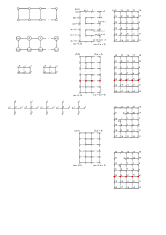
(a) $6\times 5$

(b) $7\times 5$

Figure 11: Equivalent networks after removing $X$

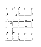
(a) $6\times 5$

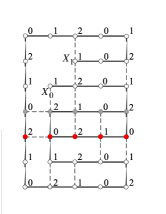
(b) $7\times 5$

Figure 12: Colored graph of the equivalent networks

(a) Numbering

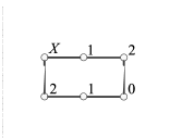
(b) Colored Graph

Figure 13: A $2\times 3$ network example

Example

We first illustrate what happens when applying this schedule to a simple $2\times 3$ grid network. The source is located at (0,0). Fig. 13a shows the numbering of this network and Fig. 13b shows the corresponding colored graph. Although node 1 and node 4 can overhear each other, they are of the same color and thus transmit at the same time. Hence they will not interfere each other. The network turns into a ring after coloring. In this example, we set all transmit coefficients $\alpha_{k}$ to $1$. The transmissions of our ternary schedule are the same as those shown in Table I for the six-node ring example.

It can be observed that the two virtual sources node 1 and node 5 always have $x_{0}(0),...,x_{0}(t)$ and $x_{1}(0),...,x_{1}(t)$ by the end of round $t$. Therefore they can always derive $x_{0}(t+1)$ and $x_{1}(t+1)$ by the end of round $t+1$ even if they receive PNC packets during round $t+1$, because they know all but one of the unknowns (native packets).

In this example, each node can obtain two native packets in a round. In a general grid network where there is interference among nodes, obtaining native packets as such cannot be guaranteed. However, as will be shown, we could ensure every non-source node still obtains two linearly independent equations in each round.

In a general grid network, depending on its position in the grid, a node can have up to four neighbors. With the Hamiltonian Node Coloring, it is possible for a node to have two or three neighbors of the same color, one of which is an adjacent node on the Hamiltonian cycle (see Section VI-B on Hamiltonian Node Coloring). When multiple neighbors of the same color transmit simultaneously, the node receives a PNC packet, for which the XOR of the simultaneous transmissions of the neighbors of the same color is received. For example, in Fig. 9b, node 9 (color-0) has four neighbors: node 8 (color-2), node 8* (color-2), node 10 (color-1) and node 20 (color-2). As a consequence, in each round node 9 receives from three nodes simultaneously in the color-2 time slot, which yields a PNC packet; it receives from only one neighbor in the color-1 time slot. For both packets, we need to make sure:

1. the packet received is linearly independent with all packets previously received;

2. the packet received is not null.

VI-D Random Transmit Coefficients

In the previous simple $2\times 3$ example, the transmit coefficients $\alpha_{k}$ for all non-source nodes were set to $1$. In a general grid, this scheme may not work. Henceforth, we consider a time-varying random transmit coefficient scheme. Specifically, the transmit coefficient $\alpha_{k}(t)$ of node $k$ in round $t$ is chosen uniform-randomly from the non-zero elements of $GF(2^{s})$, and $\alpha_{k}(t)$ for different $k$ and $t$ are i.i.d. The sequences of packets $\{x_{0}(t)\}_{t=0,1,2,...}$ and $\{x_{1}(t)\}_{t=0,1,2,...}$ transmitted by the virtual sources $X_{0}$ and $X_{1}$ remain the same, and their transmit coefficients can be considered as 1 throughout the process.

In grid networks, the newest information (i.e., signals embedded with the latest native packets) come through a shortest path from the the virtual sources $X_{0}$ and $X_{1}$, and in general this shortest path may not be along the Hamiltonian cycle.

Definition 13 (Shortest Path).

A shortest path from a virtual source to a node is a shortest sequence of adjacent nodes leading from the virtual source to the node in the colored graph of the grid network.

Note that in general there could be multiple shortest paths of the same length leading from a virtual source to a node, and some of them may share some common intermediate nodes.

Definition 14 (Coefficient Product/Path Coefficient).

The coefficient product of $p=k_{1}-k_{2}-...-k_{l}-k$, a path from node $k_{1}$ to node $k$, in round $t$ is

$$g_{p}(t)= \alpha_{k_{1}}(t-(l-1))\alpha_{k_{2}}(t-(l-2))$$

$$...\alpha_{k_{l-1}}(t-1)\alpha_{k_{l}}(t)$$ (24)

$$= \prod_{r=1}^{l}\alpha_{k_{r}}(t-(l-r)),$$ (25)

where $\alpha_{k_{1}}(t-(l-1)),\alpha_{k_{2}}(t-(l-2),...,\alpha_{k_{l-1}}(t-1),\alpha_{k_{l}}(t)$ are the transmit coefficients of nodes $k_{1},k_{2},...,k_{l-1},k_{l}$ in rounds $t-(l-1),t-(l-2),...,t-1,t$, respectively. We will use the terms “coefficient product” and “path coefficient” interchangeably in this paper.

If a native packet $x$ goes through a path $p$, then its coefficient when it arrives at the last node in round $t$ will be $g_{p}(t)$, the coefficient product (path coefficient) of this path.

Definition 15 (Aggregated Path Coefficient).

If a packet $x$ begins its journey from a node $j$ with an initial transmit coefficient $\alpha_{j}$, splits and travels over multiple paths $p_{1},p_{2},...$ of the same length, and then arrives at the same node $k$ in the same time slot in round $t$, then the coefficient of the packet $x$ when it is received at node $k$ is the sum of coefficient products $\alpha_{j}g_{p_{1}}(t)\oplus\alpha_{j}g_{p_{2}}(t)\oplus...$, thanks to PNC. This sum of coefficient products will be referred to as the aggregated path coefficient.

Example of received packets

For example in Fig. 9b, in time slot $3t$, node 10 receives from node 9. The shortest path from $X_{0}$ to node $10$ for this time slot is $p_{0}=1-8-9-10$. However, this is the shortest path for $\{x_{0}(t)\}_{t=0,1,...}$ only, because node $1$ only transmits $\{\alpha_{1}(t)x_{0}(t)\}_{t=0,1,...}$. The shortest paths from $X_{1}$ to node $10$ for $\{x_{1}(t)\}_{t=0,1,...}$ are $p_{1}=31-2-1-8-9-10$, $p_{2}=31-2-7-8-9-10$ and $p_{3}=31-2-7-8^{*}-9-10$. A native packet in $\{x_{0}(t)\}_{t=0,1,...}$ will be multiplied by the transmit coefficient of the sender when being sent. The packet node $10$ receives from node $9$ in time slot $3t$ is

$$r_{0}^{10}(t)= g_{p_{0}}(t)x_{0}(t-3)$$

$$\oplus(g_{p_{1}}(t)\oplus g_{p_{2}}(t)\oplus g_{p_{3}}(t))x_{1}(t-5)$$

$$\oplus\epsilon(x_{0}(t-4),x_{0}(t-5),...,x_{0}(0))$$

$$\oplus\epsilon(x_{1}(t-6),x_{1}(t-7),...,x_{1}(0))$$ (26)

$$= \alpha_{1}(t-2)\alpha_{8}(t-1)\alpha_{9}(t)x_{0}(t-3)$$

$$\oplus(\alpha_{31}(t-4)\alpha_{2}(t-3)\alpha_{1}(t-2)\alpha_{8}(t-1)\alpha_{9}(t)$$

$$\oplus\alpha_{31}(t-4)\alpha_{2}(t-3)\alpha_{7}(t-2)\alpha_{8}(t-1)\alpha_{9}(t)$$

$$\oplus\alpha_{31}(t-4)\alpha_{2}(t-3)\alpha_{7}(t-2)\alpha_{8^{*}}(t-1)\alpha_{9}(t))$$

$$x_{1}(t-5)$$

$$\oplus\epsilon(x_{0}(t-4),x_{0}(t-5),...,x_{0}(0))$$

$$\oplus\epsilon(x_{1}(t-6),x_{1}(t-7),...,x_{1}(0))$$ (27)

where $\epsilon(\cdot)$ is a linear combination of the arguments. We see that the coefficient associated with a native packet embedded in a reception is in general an aggregated path coefficient.

The time indexes of the newest native packets in Eqn. (27) escalate over time. Therefore each new $r_{0}^{10}(t)$ is linearly independent of all $r_{0}^{10}(t^{\prime}),t^{\prime}<t$.

Packet $r_{1}^{10}(t)$, the packet node 10 receives in time slot $3t+2$, will be a PNC packet from nodes 11 and 17. A shortest path in this time slot for $\{x_{0}(t)\}_{t=0,1,...}$ is $1-8-21-20-19-18-17-10$; and a shortest path for $\{x_{1}(t)\}_{t=0,1,2,...}$ is $31-2-7-8^{*}-7^{*}-12-11-10$. Therefore the newest native packets in it would be $x_{0}(t-7)$ and $x_{1}(t-7)$, each multiplied by some $\bigoplus_{p\in S}g_{p}(t)$, where $S$ is the set of all shortest paths and $p$ is a shortest path for the native packet. Note that for time slot $3t+2$, an even shorter path exists for $\{x_{0}(t)\}_{t=0,1,...}$: 1-8-9-10-17-10. However, this path has a loop and in general we do not consider paths with loops because they can be eliminated in our computation for the solution. For this path, a packet is sent from node 10 and cycled back from node 17. The cycled back packet is $\alpha_{17}(t)r_{0}^{10}(t-1)+...$, in which $\alpha_{17}(t)r_{0}^{10}(t-1)$ is the coefficient of node 17 times a packet already received by node 10, thus can be removed easily. In fact, any cycled back information can be removed with the knowledge of nodes on the cycle and the packets previously received. Therefore, we only consider shortest paths with no cycles in this work.

Packets received by a general node

We now give a general expression for received packets. Consider a general node $k,k\neq 1\mbox{ or }MN-1$, in the network. Focus on one of its two receiving time slots in round $t$. Let $S_{0},S_{1}$ be the sets of shortest paths for $\{x_{0}(t)\}_{t=0,1,...}$ and $\{x_{1}(t)\}_{t=0,1,...}$, respectively, in this time slot; and $S_{0}^{+q},S_{1}^{+q}$ be the sets of paths that are $q$ hops longer than $S_{0}$ and $S_{1}$ for $\{x_{0}(t)\}_{t=0,1,...}$ and $\{x_{1}(t)\}_{t=0,1,...}$, respectively. Depending on $q$, each of $S_{0}^{+q}$ and $S_{1}^{+q}$ may or may not be empty. Node $k$ receives

$$r_{0}^{k}(t)= a_{S_{0}}(t)x_{0}(t-i_{0})\oplus a_{S_{0}^{+1}}(t)x_{0}(t-i_{0}-1)$$

$$\oplus...\oplus a_{S_{0}^{+t-i_{0}}}(t)x_{0}(0)$$

$$\oplus a_{S_{1}}(t)x_{1}(t-i_{1})\oplus a_{S_{1}^{+1}}(t)x_{1}(t-i_{1}-1)$$

$$\oplus...\oplus a_{S_{1}^{+t-i_{1}}}(t)x_{1}(0),$$ (28)

where $i_{0}$ and $i_{1}$ are the lengths of paths in $S_{0}$ and $S_{1}$, respectively; and where the aggregated path coefficients are given by

$$a_{S_{0}}(t)=\bigoplus_{p\in S_{0}}g_{p}(t),\;a_{S_{1}}(t)=\bigoplus_{p\in S_{1}}g_{p}(t),$$ (29)

$$a_{S_{0}^{+q}}(t)=\bigoplus_{p\in S_{0}^{+q}}g_{p}(t),\;a_{S_{1}^{+q}}(t)=\bigoplus_{p\in S_{1}^{+q}}g_{p}(t).$$ (30)

Grouping the packets received in this colored slot in all rounds, we have a linear equation system $\{r_{0}^{k}(t)\}_{t\geq\min(i_{0},i_{1})}$.

Now consider the other receiving time slot of node $k$ in round $t$. Let $T_{0},T_{1}$ be the sets of shortest paths for $\{x_{0}(t)\}_{t=0,1,...}$ and $\{x_{1}(t)\}_{t=0,1,...}$, respectively, in this time slot; and $T_{0}^{+q},T_{1}^{+q}$ be the sets of paths that are $q$ hops longer than $T_{0}$ and $T_{1}$ for $\{x_{0}(t)\}_{t=0,1,...}$ and $\{x_{1}(t)\}_{t=0,1,...}$, respectively. Node $k$ receives

$$r_{1}^{k}(t)= a_{T_{0}}(t)x_{0}(t-j_{0})\oplus a_{T_{0}^{+1}}(t)x_{0}(t-j_{0}-1)$$

$$\oplus...\oplus a_{T_{0}^{+t-j_{0}}}(t)x_{0}(0)$$

$$\oplus a_{T_{1}}(t)x_{1}(t-j_{1})\oplus a_{T_{1}^{+1}}(t)x_{1}(t-j_{1}-1)$$

$$\oplus...\oplus a_{T_{1}^{+t-j_{1}}}(t)x_{1}(0),$$ (31)

where $j_{0}$ and $j_{1}$ are the lengths of paths in $T_{0}$ and $T_{1}$, respectively; and where the aggregated path coefficients are given by

$$a_{T_{0}}(t)=\bigoplus_{p\in T_{0}}g_{p}(t),\;a_{T_{1}}(t)=\bigoplus_{p\in T_{1}}g_{p}(t),$$ (32)

$$a_{T_{0}^{+q}}(t)=\bigoplus_{p\in T_{0}^{+q}}g_{p}(t),\;a_{T_{1}^{+q}}(t)=\bigoplus_{p\in T_{1}^{+q}}g_{p}(t).$$ (33)

Grouping the packets received in this colored slot in all rounds, we have another linear equation system $\{r_{1}^{k}(t)\}_{t\geq\min(j_{0},j_{1})}$.

Note that we do not consider paths with cycles, because they can be eliminated in our computation for the solution. For example, if a packet $y^{k}(t)$ sent by node $k$ in round $t$ is cycled back via a path $k-k_{1}-k_{2}-...-k_{l}-k$, then the resulting component in a packet received in round $t+l$ will be $\alpha_{k_{1}}(t+1)\alpha_{k_{2}}(t+2)...\alpha_{k_{l}}(t+l)y^{k}(t)$, which can be eliminated from the packet, as node $k$ already knows $y^{k}(t)$. In other words, cycle-back information does not contain anything new.

Each of the virtual sources, $X_{0}$ or $X_{1}$, broadcasts $D/2$ native packets (assuming $D$ is even for simplicity). That is, $\{x_{0}(t)\}_{t=0,1,...}=\{x_{0}(t)\}_{t=0,1,...,\frac{D}{2}-1}$ and $\{x_{1}(t)\}_{t=0,1,...}=\{x_{1}(t)\}_{t=0,1,...,\frac{D}{2}-1}$. After all native packets have been sent by the source, we allow $MN$ more time slots for them to circulate in the network. During these $MN$ time slots, the source and the virtual sources can be considered as transmitting null packets, which do not increase the number of unknowns in the network.

We select $\{r_{0}^{k}(t_{0})\}_{\min(i_{0},i_{1})\leq t_{0}\leq\max(i_{0},i_{1})+\frac{D}{2}-1}$, a subset of $\{r_{0}^{k}(t)\}_{t\geq\min(i_{0},i_{1})}$, and $\{r_{1}^{k}(t_{1})\}_{\min(j_{0},j_{1})\leq t_{1}\leq\max(j_{0},j_{1})+\frac{D}{2}-1}$, a subset of $\{r_{1}^{k}(t)\}_{t\geq\min(j_{0},j_{1})}$, and group them together as a single linear equation system

$$\{r_{0}^{k}(t_{0}),r_{1}^{k}(t_{1})\}_{\begin{subarray}{c}\min(i_{0},i_{1})\leq t_{0}\leq\max(i_{0},i_{1})+\frac{D}{2}-1\\ \min(j_{0},j_{1})\leq t_{1}\leq\max(j_{0},j_{1})+\frac{D}{2}-1\end{subarray}}.$$ (34)

Before we discuss the relationship between the equations, we introduce some additional definitions. In the following, we will use $|p|$ to represent the length of a path $p$, i.e., the number of hops in $p$.

Definition 16 (Equal-hop Path Set).

An equal-hop path set $S$ is a set of paths of the same length. For example $S=\{p_{1},p_{2},...\}$, where $|p_{1}|=|p_{2}|=...$, is an equal-hop path set.

Definition 17 ($\bm{h}$-hop Path Set).

An equal-hop path set $S$ is called an $h$-hop path set if all paths $p\in S$ have the same length $|p|=h$.

Conjecture 1.

Consider a node $k$ that is not the source or one of the virtual sources. Let $i_{0}$, $i_{1}$, $j_{0}$, $j_{1}$ be as defined in Eqn. (28) and (31). Suppose that $c_{0}$ and $c_{1}$ are the two colors different from the color of $k$. Also suppose that $i_{1}-i_{0}=j_{1}-j_{0}$. Then node $k$ always has two disjoint shortest paths $p_{0}$ and $p_{1}$ such that: 1) $p_{0}$ is from $X_{0}$ through the color-$c_{0}$ neighbors, and $p_{1}$ is from $X_{1}$ through the color-$c_{1}$ neighbors, to node $k$; or 2) $p_{0}$ is from $X_{0}$ through the color-$c_{1}$ neighbors, and $p_{1}$ is from $X_{1}$ through the color-$c_{0}$ neighbors, to node $k$.

The verification of the conjecture is shown in Appendix -D. Although we cannot prove the conjecture, we verify with a computer program that the conjecture is true for a large number of networks.

Corollary 1 (of Conjecture 1).

Let $a_{S_{0}}(t)$, $a_{S_{1}}(t)$, $a_{T_{0}}(t)$, $a_{T_{1}}(t)$ be as defined in Eqn. (29) and (32), and let $i_{0}$, $i_{1}$, $j_{0}$, $j_{1}$ be defined as in Eqn. (28) and (31). Suppose that $i_{0}<i_{1}$, $j_{0}<j_{1}$ and $i_{1}-i_{0}=j_{1}-j_{0}$, then $a_{S_{0}}(i_{1})a_{T_{1}}(j_{1})\oplus a_{S_{1}}(i_{1})a_{T_{0}}(j_{1})\not\equiv 0$.

The proof of the corollary is in Appendix -C.

Remark: Note that in Corollary 1 and the subsequent discussion, we use the equivalent sign $\equiv$ to mean the equivalence of the two expressions on the LHS and the RHS. In Corollary 1, $a_{S_{0}}(i_{1})a_{T_{1}}(j_{1})\oplus a_{S_{1}}(i_{1})a_{T_{0}}(j_{1})\not\equiv 0$ means the variables inside the expression on the LHS does not cancel out to zero. In our scheme, transmit coefficients are i.i.d. uniform random variables with values drawn from $GF(2^{s})\backslash\{0\}$. It is entirely possible that a given set of realizations for the transmit coefficients causes the above the expression to be 0. However, not all realizations do so if the expression is not identically equal to 0.

Corollary 2 (of Conjecture 1).

We can derive all native packets from (34) with probability greater than $(1-2MN/(2^{s}-1))^{D/2}$.

Proof:

We first note that we can solve for $\{x_{0}(t)\}_{0\leq t<i_{1}-i_{0}}$ from

$$\{r_{0}^{k}(t_{0})\}_{\min(i_{0},i_{1})\leq t_{0}<\max(i_{0},i_{1})}$$

alone without considering $r_{1}^{k}(t_{1})$ when $i_{0}<i_{1}$ as long as $a_{S_{0}}(t_{0})\neq 0$ for all $\min(i_{0},i_{1})\leq t_{0}<\max(i_{0},i_{1})$, or $\{x_{1}(t)\}_{0\leq t<i_{0}-i_{1}}$ from the above when $i_{0}>i_{1}$ as long as $a_{S_{1}}(t_{0})\neq 0$ for all $\min(i_{0},i_{1})\leq t_{0}<\max(i_{0},i_{1})$. Similarly we can solve for $\{x_{0}(t)\}_{0\leq t<j_{1}-j_{0}}$ from

$$\{r_{1}^{k}(t_{1})\}_{\min(j_{0},j_{1})\leq t_{1}<\max(j_{0},j_{1})}$$

alone without considering $r_{0}^{k}(t_{0})$ when $j_{0}<j_{1}$ as long as $a_{T_{0}}(t_{1})\neq 0$ for all $\min(j_{0},j_{1})\leq t_{1}<\max(j_{0},j_{1})$, or $\{x_{1}(t)\}_{0\leq t<j_{0}-j_{1}}$ from the above when $j_{0}>j_{1}$ as long as $a_{T_{1}}(t_{1})\neq 0$ for all $\min(j_{0},j_{1})\leq t_{1}<\max(j_{0},j_{1})$. We only need to consider $r_{0}^{k}(t)$ and $r_{1}^{k}(t)$ together when solving $x_{0}(t)$ or $x_{1}(t)$ for large $t$.

There are several cases depending on $i_{0}$, $i_{1}$, $j_{0}$ and $j_{1}$:

1. $i_{0}<i_{1}$ and $j_{0}>j_{1}$:

We can solve for $\{x_{0}(t)\}_{0\leq t<i_{1}-i_{0}}$ from $\{r_{0}^{k}(t_{0})\}_{\min(i_{0},i_{1})\leq t_{0}<\max(i_{0},i_{1})}$ as long as $a_{S_{0}}(t_{0})\neq 0$ for all $\min(i_{0},i_{1})\leq t_{0}<\max(i_{0},i_{1})$, and $\{x_{1}(t)\}_{0\leq t<j_{0}-j_{1}}$ from $\{r_{1}^{k}(t_{1})\}_{\min(j_{0},j_{1})\leq t_{1}<\max(j_{0},j_{1})}$ as long as $a_{S_{1}}(t_{1})\neq 0$ for all $\min(j_{0},j_{1})\leq t_{1}<\max(j_{0},j_{1})$.

We express $a_{S_{0}}(t_{0})$ by

$$a_{S_{0}}(t_{0})=P_{1}\oplus P_{2}\oplus...\oplus P_{L}$$ (35)

where each of $\{P_{j}\}_{j=1,2,...,L}$ is a path coefficient, i.e.,

$$P_{j}=g_{p}(t_{0})$$

for some $p\in S_{0}$. Each of $\{P_{j}\}_{j=1,2,...,L}$ is a product of $R=i_{0}$ transmit coefficients, i.e.,

$$P_{j}=g_{p}(t_{0})=\prod_{u\mbox{ is in }p}\alpha_{u}(t_{u})$$

where $t_{u}$ is the round node $u$ is visited. Each $P_{j}$ contains $R=i_{0}$ factors. A path cannot have more than $MN$ hops, as $MN$ is the number of nodes in the network. Thus, $R=i_{0}\leq MN$. Without loss of generality, suppose $P_{1}$ contains a set of distinct factors that is not exactly the same as that of any $P_{j},2\leq j\leq L$. Such $P_{1}$ exists because no two shortest paths contain the same set of nodes. By Lemma 1 in Appendix -C, $a_{S_{0}}(t_{0})\not\equiv 0$; by Lemma 2 in Appendix -C,

$$\Pr\left(a_{S_{0}}(t_{0})=0\right) =\Pr\left(P_{1}\oplus P_{2}\oplus...\oplus P_{L}=0\right)$$

$$\leq\frac{R}{2^{s}-1}\leq\frac{MN}{2^{s}-1},$$

i.e.,

$$\Pr\left(a_{S_{0}}(t_{0})\neq 0\right)>1-MN/(2^{s}-1).$$

By similar argument, we have $a_{T_{1}}(t_{1})\not\equiv 0$ and

$$\Pr\left(a_{T_{1}}(t_{1})\neq 0\right)>1-MN/(2^{s}-1).$$

Thus, we can solve for $\{x_{0}(t)\}_{0\leq t<i_{1}-i_{0}}$ from $\{r_{0}^{k}(t_{0})\}_{\min(i_{0},i_{1})\leq t_{0}<\max(i_{0},i_{1})}$ with probability greater than $(1-MN/(2^{s}-1))^{i_{1}-i_{0}}$, and $\{x_{1}(t)\}_{0\leq t<j_{0}-j_{1}}$ from $\{r_{1}^{k}(t_{1})\}_{\min(j_{0},j_{1})\leq t_{1}<\max(j_{0},j_{1})}$ with probability $(1-MN/(2^{s}-1))^{j_{0}-j_{1}}$.

The first pair of equations that cannot be solved from its own series is

$$r_{0}^{k}(i_{1})= a_{S_{0}}(i_{1})x_{0}(i_{1}-i_{0})\oplus a_{S_{0}^{+1}}(i_{1})x_{0}(i_{1}-i_{0}-1)$$

$$\oplus...\oplus a_{S_{0}^{+i_{1}-i_{0}}}(i_{1})x_{0}(0)$$

$$\oplus a_{S_{1}}(i_{1})x_{1}(0)$$

$$r_{1}^{k}(j_{0})= a_{T_{0}}(j_{0})x_{0}(0)\oplus$$

$$\oplus a_{T_{1}}(j_{0})x_{1}(j_{0}-j_{1})\oplus a_{T_{1}^{+1}}(j_{0})x_{1}(j_{0}-j_{1}-1)$$

$$\oplus...\oplus a_{T_{1}^{+j_{0}-j_{1}}}(j_{0})x_{1}(0).$$

$x_{0}(i_{1}-i_{0})$ can be solved from $r_{0}^{k}(i_{1})$ as long as $a_{S_{0}}(i_{1})\neq 0$ because $x_{0}(0),...,x_{0}(i_{1}-i_{0}-1)$ and $x_{1}(0)$ are already known; and $x_{1}(j_{0}-j_{1})$ can be solved from $r_{1}^{k}(j_{0})$ as long as $a_{T_{1}}(j_{0})\neq 0$ because $x_{0}(0)$ and $x_{1}(0),...,x_{1}(j_{0}-j_{1}-1)$ are already known.

Since $\Pr\left(a_{S_{0}}(i_{1})\neq 0\right)>1-MN/(2^{s}-1)$ and $\Pr\left(a_{T_{1}}(j_{0})\neq 0\right)>1-MN/(2^{s}-1)$, we can solve for $x_{0}(i_{1}-i_{0})$ and $x_{1}(j_{0}-j_{1})$ from $r_{0}^{k}(i_{1})$ and $r_{1}^{k}(j_{0})$ with probability greater than $(1-MN/(2^{s}-1))^{2}\geq 1-2MN/(2^{s}-1)$ conditioning on that $\{x_{0}(t)\}_{0\leq t<i_{1}-i_{0}}$ and $\{x_{1}(t)\}_{0\leq t<j_{0}-j_{1}}$ are already known. Similarly $x_{0}(i_{1}-i_{0}+1)$ and $x_{1}(j_{0}-j_{1}+1)$ can be solved from $r_{0}^{k}(i_{1}+1)$ and $r_{1}^{k}(j_{0}+1)$ with probability greater than $1-2MN/(2^{s}-1)$, conditioning on that $\{x_{0}(t)\}_{0\leq t<i_{1}-i_{0}+1}$ and $\{x_{1}(t)\}_{0\leq t<j_{0}-j_{1}+1}$ are already known. By induction all native packets can be solved from the equations in (34) with probability greater than $(1-2MN/(2^{s}-1))^{D/2}$, as there are $D/2$ native packets in both $\{x_{0}(t)\}_{t=0,...,\frac{D}{2}-1}$ and $\{x_{1}(t)\}_{t=0,...,\frac{D}{2}-1}$.

2. $i_{0}>i_{1}$ and $j_{0}<j_{1}$:

The proof of this case is similar to the previous case, thus will not be discussed here.

3. $i_{0}<i_{1}$, $j_{0}<j_{1}$, and $i_{1}-i_{0}\neq j_{1}-j_{0}$:

We can solve for $\{x_{0}(t)\}_{0\leq t<i_{1}-i_{0}}$ from $\{r_{0}^{k}(t_{0})\}_{\min(i_{0},i_{1})\leq t_{0}<\max(i_{0},i_{1})}$, and $\{x_{0}(t)\}_{0\leq t<j_{1}-j_{0}}$ from $\{r_{1}^{k}(t_{1})\}_{\min(j_{0},j_{1})\leq t_{1}<\max(j_{0},j_{1})}$. Without loss of generality, assume $i_{1}-i_{0}>j_{1}-j_{0}$. The first pair of equations that cannot be solved from its own series is

$$r_{0}^{k}(i_{1})= a_{S_{0}}(i_{1})x_{0}(i_{1}-i_{0})\oplus a_{S_{0}^{+1}}(i_{1})x_{0}(i_{1}-i_{0}-1)$$

$$\oplus...\oplus a_{S_{0}^{+i_{1}-i_{0}}}(i_{1})x_{0}(0)$$

$$\oplus a_{S_{1}}(i_{1})x_{1}(0)$$

$$r_{1}^{k}(j_{1})= a_{T_{0}}(j_{1})x_{0}(j_{1}-j_{0})\oplus a_{T_{0}^{+1}}(j_{1})x_{0}(j_{1}-j_{0}-1)$$

$$\oplus...\oplus a_{T_{0}^{+j_{1}-j_{0}}}(j_{1})x_{0}(0)$$

$$\oplus a_{T_{1}}(j_{1})x_{1}(0).$$

$x_{1}(0)$ can be solved from $r_{1}^{k}(j_{1})$ as long as $a_{T_{1}}(j_{1})\neq 0$ because $x_{0}(0),...,x_{0}(j_{1}-j_{0}),...,x_{0}(i_{1}-i_{0}-1)$ are already known; then $x_{0}(i_{1}-i_{0})$ can be solved from $r_{0}^{k}(i_{1})$ as long as $a_{S_{0}}(i_{1})\neq 0$ because $x_{0}(0),...,x_{0}(i_{1}-i_{0}-1)$ and $x_{1}(0)$ are already known. With similar argument as in Case 1, all native packets can be solved from the equations in (34) with probability greater than $(1-2MN/(2^{s}-1))^{D/2}$.

4. $i_{0}>i_{1}$, $j_{0}>j_{1}$, and $i_{1}-i_{0}\neq j_{1}-j_{0}$:

The proof of this case is similar to the previous case, thus will not be discussed here.

5. $i_{0}<i_{1}$, $j_{0}<j_{1}$, and $i_{1}-i_{0}=j_{1}-j_{0}$:

Let $\delta=i_{1}-i_{0}=j_{1}-j_{0}$. We can solve for $\{x_{0}(t)\}_{0\leq t<\delta}$ from either $\{r_{0}^{k}(t_{0})\}_{\min(i_{0},i_{1})\leq t_{0}<\max(i_{0},i_{1})}$ or $\{r_{1}^{k}(t_{1})\}_{\min(j_{0},j_{1})\leq t_{1}<\max(j_{0},j_{1})}$. The first pair of equation that cannot be solved from its own series is

$$r_{0}^{k}(i_{1})= a_{S_{0}}(i_{1})x_{0}(\delta)\oplus a_{S_{0}^{+1}}(i_{1})x_{0}(\delta-1)$$

$$\oplus...\oplus a_{S_{0}^{+\delta}}(i_{1})x_{0}(0)$$

$$\oplus a_{S_{1}}(i_{1})x_{1}(0)$$

$$r_{1}^{k}(j_{1})= a_{T_{0}}(j_{1})x_{0}(\delta)\oplus a_{T_{0}^{+1}}(j_{1})x_{0}(\delta-1)$$

$$\oplus...\oplus a_{T_{0}^{+\delta}}(j_{1})x_{0}(0)$$

$$\oplus a_{T_{1}}(j_{1})x_{1}(0).$$

Putting the unknown part on the LHS and known part on the RHS yields

$$a_{S_{0}}(i_{1})x_{0}(\delta)\oplus a_{S_{1}}(i_{1})x_{1}(0)= r_{0}^{k}(i_{1})\oplus a_{S_{0}^{+1}}(i_{1})x_{0}(\delta-1)$$

$$\oplus...\oplus a_{S_{0}^{+\delta}}(i_{1})x_{0}(0)$$

$$a_{T_{0}}(j_{1})x_{0}(\delta)\oplus a_{T_{1}}(j_{1})x_{1}(0)= r_{1}^{k}(j_{1})\oplus a_{T_{0}^{+1}}(j_{1})x_{0}(\delta-1)$$

$$\oplus...\oplus a_{T_{0}^{+\delta}}(j_{1})x_{0}(0).$$

As long as the matrix

$$\left(\begin{array}[]{cc}a_{S_{0}}(i_{1})&a_{S_{1}}(i_{1})\\ a_{T_{0}}(j_{1})&a_{T_{1}}(j_{1})\end{array}\right)$$

has full rank, we can solve for $x_{0}(\delta)$ and $x_{1}(0)$ from the two equations. The determinant of the matrix is

$$A =\det\left(\begin{array}[]{cc}a_{S_{0}}(i_{1})&a_{S_{1}}(i_{1})\\ a_{T_{0}}(j_{1})&a_{T_{1}}(j_{1})\end{array}\right)$$ (38)

$$=a_{S_{0}}(i_{1})a_{T_{1}}(j_{1})\oplus a_{S_{1}}(i_{1})a_{T_{0}}(j_{1}).$$ (39)

$A\not\equiv 0$ (i.e., $A$ is not always equal to zero) by Appendix -C.

We express $A$ by

$$A=Q_{1}\oplus Q_{2}\oplus...\oplus Q_{L}$$ (40)

where each of $\{Q_{j}\}_{j=1,2,...,L}$ is a product of two path coefficients, i.e.,

$$Q_{j}=g_{p}(i_{1})g_{p^{\prime}}(j_{1})$$

for some $p\in S_{0}$ and $p^{\prime}\in T_{1}$, or $p\in S_{1}$ and $p^{\prime}\in T_{0}$. Each of $\{Q_{j}\}_{j=1,2,...,L}$ is a product of $R=i_{1}+j_{0}=i_{0}+j_{1}$ transmit coefficients, i.e.,

$$Q_{j}=g_{p}(i_{1})g_{p^{\prime}}(j_{1})=\prod_{u\mbox{ is in }p}\alpha_{u}(t_{u})\prod_{v\mbox{ is in }p^{\prime}}\alpha_{v}(t_{v})$$

where $t_{u}$ and $t_{v}$ are the rounds node $u$ and $v$ are visited, respectively. Each $Q_{j}$ contains $R$ factors. A path cannot have more than $MN$ hops, as $MN$ is the number of nodes in the network. Thus, $R=i_{1}+j_{0}=i_{0}+j_{1}\leq 2MN$. Without loss of generality, suppose $Q_{1}$ contains a set of distinct factors that is not exactly the same as that of any $Q_{j},2\leq j\leq L$. Such $Q_{1}$ is showed to exist in Appendix -C. Also, without loss of generality, we assume if $Q_{j}=Q_{k}$ for $j,k\neq 1$, then they will be removed from $Q_{1}\oplus Q_{2}\oplus...\oplus Q_{L}$ so that $Q_{j}\neq Q_{k}$ in the remaining $Q_{1}\oplus Q_{2}\oplus...\oplus Q_{L}$. We write

$$Q_{1}=\prod_{m=1}^{R}r_{m},$$

where $r_{m}$ is $\alpha_{u}(t_{u})$ for some $u$ in $p$ or $\alpha_{v}(t_{v})$ for some $v$ in $p^{\prime}$, and $r_{m_{1}}\neq r_{m_{2}}$ for $m_{1}\neq m_{2},1\leq m_{1},m_{2}\leq R$. By Lemma 2, $\Pr\left(A=0\right)=\Pr\left(Q_{1}\oplus Q_{2}\oplus...\oplus Q_{L}=0\right)\leq R/(2^{s}-1)\leq 2MN/(2^{s}-1)$.

Therefore, we can solve for $x_{0}(\delta)$ and $x_{1}(0)$ from $r_{0}^{k}(i_{1})$ and $r_{1}^{k}(j_{1})$ with probability greater than $1-2MN/(2^{s}-1)$. Similarly, we can solve for $x_{0}(\delta+1)$ and $x_{1}(2)$ from

$$r_{0}^{k}(i_{1}+1)= a_{S_{0}}(i_{1}+1)x_{0}(\delta+1)\oplus a_{S_{0}^{+1}}(i_{1}+1)x_{0}(\delta)$$

$$\oplus...\oplus a_{S_{0}^{+\delta+1}}(i_{1}+1)x_{0}(0)$$

$$\oplus a_{S_{1}}(i_{1}+1)x_{1}(1)\oplus a_{S_{1}^{+1}}(i_{1}+1)x_{1}(0)$$

$$r_{1}^{k}(j_{1}+1)= a_{T_{0}}(j_{1}+1)x_{0}(\delta+1)\oplus a_{T_{0}^{+1}}(j_{1}+1)x_{0}(\delta)$$

$$\oplus...\oplus a_{T_{0}^{+\delta+1}}(j_{1}+1)x_{0}(0)$$

$$\oplus a_{T_{1}}(j_{1}+1)x_{1}(1)\oplus a_{T_{1}^{+1}}(j_{1}+1)x_{1}(0)$$

with probability greater than $1-2MN/(2^{s}-1)$, conditioning on that $\{x_{0}(t)\}_{0\leq t<\delta+1}$ and $x_{1}(0)$ are already known. By induction all native packets can be solved from the equations in (34) with probability greater than $(1-2MN/(2^{s}-1))^{D/2}$, as there are $D/2$ native packets in both $\{x_{0}(t)\}_{t=0,...,\frac{D}{2}-1}$ and $\{x_{1}(t)\}_{t=0,...,\frac{D}{2}-1}$.

6. $i_{0}>i_{1}$, $j_{0}>j_{1}$, and $i_{0}-i_{1}=j_{0}-j_{1}$:

The proof of this case is similar to the previous case, thus will not be discussed here.

In conclusion, all native packets can be solved from (34) with probability greater than $(1-2MN/(2^{s}-1))^{D/2}$. ∎

With the above lemmas, we can show that the broadcast throughput upper bound is achievable in grid networks with high probability. This result is presented in the following theorem.

Corollary 3 (of Conjecture 1).

Suppose that $M$ and $N$ are fixed. The broadcast throughput in grid networks reaches $2/3$ with high probability when $s$ is of order larger than $\log D$.

Proof:

By Corollary 2, all native packets can be solved from (34) with probability greater than

$$(1-\frac{2MN}{2^{s}-1})^{\frac{D}{2}}.$$ (41)

For large $s$, $(1-\frac{2MN}{2^{s}-1})^{\frac{D}{2}}$ can be approximated by

$$\exp(-\frac{MND}{2^{s}-1}).$$ (42)

Thus, if $s$ is of order larger than $\log D$ (e.g., $s=\log D^{e}$), where $e>1$, the limit of the above probability as $D\to\infty$ is

$$\lim_{D\to\infty}(1-\frac{2MN}{2^{s}-1})^{\frac{D}{2}}=1.$$ (43)

Therefore if $D$ is large, at the end of round $(D/2+\max(i_{0},i_{1})-1)$, node $k$ can derive all native packets from $X$ with a high probability. At the end of round $D/2+MN-2$, all nodes can derive all native packets from $X$ with a high probability. The throughput is

$$\rho=\lim_{D\to\infty}\frac{D}{3(\frac{D}{2}+MN-2)}=\frac{2}{3}.$$ (44)

∎

As a consequence, the broadcast throughput upper bound is achievable with high probability when the field size is of order larger than the logarithm of the number of packets.

VII Conclusions

In this work, we have investigated the broadcast throughput of half-duplex wireless networks. We show that the theoretical throughput upper bound is $n/(n+1)$ for single-source broadcast, where $n$ is the minimum vertex-cut size of the network. This upper bound is not always achievable in general, but is achievable in many networks, including line, ring, chord ring, and grid networks.

-A Broadcast throughput of the network in Fig. 2

In this appendix, we argue that the broadcast throughput in the network in Fig. 2 cannot reach the upper bound given by Theorem 1. Let $\mathcal{T}_{i}$ be the set of time slots during which node $i$ transmits within the $W_{D}$ time slots; let $\mathcal{R}_{i}$ be the set of time slots during which node $i$ receives within the $W_{D}$ time slots.

To achieve the the throughput upper bound $2/3$, we need

$$|\mathcal{R}_{i}|\geq\frac{2}{3}W_{D},\forall i\in\{X_{0},X_{1},1,2,3\}.$$

Since a node is either in the transmission mode or the receiving mode, we have

$$|\mathcal{T}_{i}|=W_{D}-|\mathcal{R}_{i}|\leq\frac{1}{3}W_{D},\forall i\in\{X_{0},X_{1},1,2,3\}.$$ (45)

Consider node 1. Its throughput is upper-bounded as follows:

$$\rho_{1} \leq|\mathcal{T}_{X_{0}}\cup\mathcal{T}_{X_{1}}|=|\mathcal{T}_{X_{0}}|+|\mathcal{T}_{X_{1}}|-|\mathcal{T}_{X_{0}}\cap\mathcal{T}_{X_{1}}|$$

$$\leq\frac{2}{3}W_{D}-|\mathcal{T}_{X_{0}}\cap\mathcal{T}_{X_{1}}|$$

In order that $\rho_{1}\geq\frac{2}{3}W_{D}$, we need

$$|\mathcal{T}_{X_{0}}\cap\mathcal{T}_{X_{1}}|=0.$$ (46)

Applying the same argument on nodes 2 and 3 gives

$$|\mathcal{T}_{X_{0}}\cap\mathcal{T}_{3}|=0$$ (47)

$$|\mathcal{T}_{X_{1}}\cap\mathcal{T}_{2}|=0$$ (48)

The throughput of node 2 is

$$\rho_{2} \leq|\mathcal{T}_{X_{0}}|+|\mathcal{T}_{3}|-|\mathcal{T}_{X_{0}}\cap\mathcal{T}_{2}|$$ (49)

$$\leq\frac{2}{3}W_{D}-|\mathcal{T}_{X_{0}}\cap\mathcal{T}_{2}|$$ (50)

$$\Rightarrow |\mathcal{T}_{X_{0}}\cap\mathcal{T}_{2}|=0$$ (51)

In the above, (49) is from the half-duplex constraint that when node 2 transmits during the $T_{2}$ slots, if $X_{0}$ transmits at the same time, no information can be received. (50) is derived from (45). Similarly, we can argue that

$$|\mathcal{T}_{X_{1}}\cap\mathcal{T}_{3}| =0$$ (52)

$$|\mathcal{T}_{2}\cap\mathcal{T}_{3}| =0$$ (53)

Now, as $W_{D}$ is the total number of time slots under consideration, we have

$$|\mathcal{T}_{X_{0}}\cup\mathcal{T}_{3}\cup\mathcal{T}_{X_{1}}\cup\mathcal{T}_{2}|\leq W_{D}$$

$$\Rightarrow |\mathcal{T}_{X_{0}}\cup\mathcal{T}_{3}|+|\mathcal{T}_{X_{1}}\cup\mathcal{T}_{2}|-|(\mathcal{T}_{X_{0}}\cup\mathcal{T}_{3})\cap(\mathcal{T}_{X_{1}}\cup\mathcal{T}_{2})|\leq W_{D}$$

In order that $\rho_{2}=\frac{2}{3}W_{D}$ and $\rho_{3}=\frac{2}{3}W_{D}$, we need

$$|\mathcal{T}_{X_{0}}\cup\mathcal{T}_{3}|\geq\frac{2}{3}W_{D}$$

$$|\mathcal{T}_{X_{1}}\cup\mathcal{T}_{2}|\geq\frac{2}{3}W_{D}$$

This is because a node can receive information from the transmissions of its neighbors only. Therefore,

$$|(\mathcal{T}_{X_{0}}\cup\mathcal{T}_{3})\cap(\mathcal{T}_{X_{1}}\cup\mathcal{T}_{2})|\geq\frac{1}{3}W_{D}$$

$$\Rightarrow |(\mathcal{T}_{X_{0}}\cap\mathcal{T}_{X_{1}})\cup(\mathcal{T}_{X_{0}}\cap\mathcal{T}_{2})\cup(\mathcal{T}_{3}\cap\mathcal{T}_{X_{1}})\cup(\mathcal{T}_{3}\cup\mathcal{T}_{2})|\geq\frac{1}{3}W_{D}$$

$$\Rightarrow |\mathcal{T}_{X_{0}}\cap\mathcal{T}_{X_{1}}|+|\mathcal{T}_{X_{0}}\cap\mathcal{T}_{2}|+|\mathcal{T}_{3}\cap\mathcal{T}_{X_{1}}|+|\mathcal{T}_{3}\cup\mathcal{T}_{2}|\geq\frac{1}{3}W_{D}$$

$$\Rightarrow |\mathcal{T}_{X_{0}}\cap\mathcal{T}_{2}|+|\mathcal{T}_{3}\cap\mathcal{T}_{X_{1}}|+|\mathcal{T}_{3}\cup\mathcal{T}_{2}|\geq\frac{1}{3}W_{D}$$ (54)

(54) is derived from (46). However, (54) contradicts (51), (52) and (53). Therefore, the throughput upper bound cannot be achieved.

-B Transmission scheme for the chord ring network in Fig. 6

In this appendix we show a transmission scheme for the chord ring network in Fig. 6. The scheduling of nodes is shown in Table III.

Here we denote the sequence of native packets to be broadcast by $X$ by $\{x_{0}(t)\}_{t=0,1,...}$, $\{x_{1}(t)\}_{t=0,1,...}$, $\{x_{2}(t)\}_{t=0,1,...}$ and $\{x_{3}(t)\}_{t=0,1,...}$. We define a round $t,t=0,1,...$ to be a set of five time slots {$5t,5t+1,5t+2,5t+3,5t+4$}. The source $X$ transmits $x_{0}(t)$, $x_{1}(t)$, $x_{2}(t)$, $x_{3}(t)$ and $x_{0}(t)\oplus x_{1}(t)\oplus x_{2}(t)\oplus x_{3}(t)$ in time slots $5t,5t+1,5t+2,5t+3$ and $5t+4$, respectively. Node $1$ transmits $x_{0}(t-1)$ in time slot $5t$; node $2$ transmits $x_{1}(t-1)$ in time slot $5t+1$; node $4$ transmits $x_{2}(t-1)$ in time slot $5t+2$; and node $5$ transmits $x_{3}(t-1)$ in time slot $5t+3$.

From round 1 onwards, every non-source node receives sufficient information for it to derive four new native packets in each round. Thus, the broadcast throughput is $4/5$.

TABLE III: Broadcast schedule for the chord ring network in Fig. 6. “s”, “r” and “d” indicate “send”, “receive” and “derive”, respectively.

t	ts	Node $X$	Node 1	Node 2	Node 3	Node 4	Node 5
0	0	s:$x_{0}(0)$	r:$x_{0}(0)$	r:$x_{0}(0)$	-	r:$x_{0}(0)$	r:$x_{0}(0)$
	1	s:$x_{1}(0)$	r:$x_{1}(0)$	r:$x_{1}(0)$	-	r:$x_{1}(0)$	r:$x_{1}(0)$
	2	s:$x_{2}(0)$	r:$x_{2}(0)$	r:$x_{2}(0)$	-	r:$x_{2}(0)$	r:$x_{2}(0)$
	3	s:$x_{3}(0)$	r:$x_{3}(0)$	r:$x_{3}(0)$	-	r:$x_{3}(0)$	r:$x_{3}(0)$
	4	s:$x_{0}(0)$ $\oplus x_{1}(0)$ $\oplus x_{2}(0)$ $\oplus x_{3}(0)$	-	-	-	-	-
1	5	s:$x_{0}(1)$	s:$x_{0}(0)$	r:$x_{0}(0)$ $\oplus x_{0}(1)$ d:$x_{0}(1)$	r:$x_{0}(0)$	r:$x_{0}(1)$	r:$x_{0}(0)$ $\oplus x_{0}(1)$ d:$x_{1}(1)$
	6	s:$x_{1}(1)$	r:$x_{1}(0)$ $\oplus x_{1}(1)$ d:$x_{1}(1)$	s:$x_{1}(0)$	r:$x_{1}(0)$	r:$x_{1}(0)$ $\oplus x_{1}(1)$ d:$x_{1}(1)$	r:$x_{1}(1)$
	7	s:$x_{2}(1)$	r:$x_{2}(1)$	r:$x_{2}(0)$ $\oplus x_{2}(1)$ d:$x_{2}(1)$	r:$x_{2}(0)$	s:$x_{2}(0)$	r:$x_{2}(0)$ $\oplus x_{2}(1)$ d:$x_{2}(1)$
	8	s:$x_{3}(1)$	r:$x_{3}(0)$ $\oplus x_{3}(1)$ d:$x_{3}(1)$	r:$x_{3}(1)$	r:$x_{3}(0)$	r:$x_{3}(0)$ $\oplus x_{3}(1)$ d:$x_{3}(1)$	s:$x_{3}(0)$
	9	s:$x_{0}(1)$ $\oplus x_{1}(1)$ $\oplus x_{2}(1)$ $\oplus x_{3}(1)$	r:$x_{0}(1)$ $\oplus x_{1}(1)$ $\oplus x_{2}(1)$ $\oplus x_{3}(1)$ d:$x_{0}(1)$	r:$x_{0}(1)$ $\oplus x_{1}(1)$ $\oplus x_{2}(1)$ $\oplus x_{3}(1)$ d:$x_{1}(1)$	-	r:$x_{0}(1)$ $\oplus x_{1}(1)$ $\oplus x_{2}(1)$ $\oplus x_{3}(1)$ d:$x_{2}(1)$	r:$x_{0}(1)$ $\oplus x_{1}(1)$ $\oplus x_{2}(1)$ $\oplus x_{3}(1)$ d:$x_{3}(1)$
2	10	s:$x_{0}(2)$	s:$x_{0}(1)$	r:$x_{0}(1)$ $\oplus x_{0}(2)$ d:$x_{0}(2)$	r:$x_{0}(1)$	r:$x_{0}(2)$	r:$x_{0}(1)$ $\oplus x_{0}(2)$ d:$x_{1}(2)$
	11	s:$x_{1}(2)$	r:$x_{1}(1)$ $\oplus x_{1}(2)$ d:$x_{1}(2)$	s:$x_{1}(1)$	r:$x_{1}(1)$	r:$x_{1}(1)$ $\oplus x_{1}(2)$ d:$x_{1}(2)$	r:$x_{1}(2)$
	12	s:$x_{2}(2)$	r:$x_{2}(2)$	r:$x_{2}(1)$ $\oplus x_{2}(2)$ d:$x_{2}(2)$	r:$x_{2}(1)$	s:$x_{2}(1)$	r:$x_{2}(1)$ $\oplus x_{2}(2)$ d:$x_{2}(2)$
	13	s:$x_{3}(2)$	r:$x_{3}(1)$ $\oplus x_{3}(2)$ d:$x_{3}(2)$	r:$x_{3}(2)$	r:$x_{3}(1)$	r:$x_{3}(1)$ $\oplus x_{3}(2)$ d:$x_{3}(2)$	s:$x_{3}(1)$
	14	s:$x_{0}(2)$ $\oplus x_{1}(2)$ $\oplus x_{2}(2)$ $\oplus x_{3}(2)$	r:$x_{0}(2)$ $\oplus x_{1}(2)$ $\oplus x_{2}(2)$ $\oplus x_{3}(2)$ d:$x_{0}(2)$	r:$x_{0}(2)$ $\oplus x_{1}(2)$ $\oplus x_{2}(2)$ $\oplus x_{3}(2)$ d:$x_{1}(2)$	-	r:$x_{0}(2)$ $\oplus x_{1}(2)$ $\oplus x_{2}(2)$ $\oplus x_{3}(2)$ d:$x_{2}(2)$	r:$x_{0}(2)$ $\oplus x_{1}(2)$ $\oplus x_{2}(2)$ $\oplus x_{3}(2)$ d:$x_{3}(2)$

-C Proof of Corollary 1:

Proof:

Suppose the colors of the receiving node – node $k$’s neighbors are $c_{0}=(k-1)\bmod 3$ and $c_{1}=(k+1)\bmod 3$. $a_{S_{0}}(i_{1})$ and $a_{S_{1}}(i_{1})$ are the aggregated path coefficients associated with the shortest paths from $X_{0}$ and $X_{1}$, respectively, to the color-$c_{0}$ neighbors; and $a_{T_{0}}(j_{1})$ and $a_{T_{1}}(j_{1})$ are the aggregated path coefficients associated with the shortest paths from $X_{0}$ and $X_{1}$, respectively, to the color-$c_{1}$ neighbors. The summands in $a_{S_{0}}(i_{1})$, $a_{S_{1}}(i_{1})$, $a_{T_{0}}(j_{1})$ and $a_{T_{1}}(j_{1})$ are products of $i_{0}$, $i_{1}$, $j_{0}$ and $j_{1}$ transmit coefficients, respectively. Thus, the summands in $a_{S_{0}}(i_{1})a_{T_{1}}(j_{1})$ and $a_{S_{1}}(i_{1})a_{T_{0}}(j_{1})$ are products of $i_{0}+j_{1}$ and $i_{1}+j_{0}$ transmit coefficients, respectively. Note that $i_{0}+j_{1}=i_{1}+j_{0}$ by the statement of the corollary.

According to our observation in Appendix -D, we conjecture (in Conjecture 1 in the main body of this report) that node $k$ always has two disjoint shortest paths $p_{0}$ and $p_{1}$ such that $p_{0}$ is from a virtual source through the color-$c_{0}$ neighbors, and $p_{1}$ is from the other virtual source through the color-$c_{1}$ neighbors, to node $k$. By disjoint we mean there is no node that is in both of the two shortest paths.

Without loss of generality, suppose $p_{0}\in S_{0}$ and $p_{1}\in T_{1}$. We first show that there does not exist two different shortest paths $\tilde{p}_{0}$ and $\tilde{p}_{1}$ such that $g_{p_{0}}(i_{1})g_{p_{1}}(j_{1})\equiv g_{\tilde{p}_{0}}(i_{1})g_{\tilde{p}_{1}}(j_{1})$.

Suppose on the contrary that there are two different shortest paths $\tilde{p}_{0}$ and $\tilde{p}_{1}$ such that $g_{p_{0}}(i_{1})g_{p_{1}}(j_{1})\equiv g_{\tilde{p}_{0}}(i_{1})g_{\tilde{p}_{1}}(j_{1})$. Let $p_{0}=u_{1}-u_{2}-...-u_{i_{0}}-k$ and $p_{1}=v_{1}-v_{2}-...-v_{j_{1}}-k$, where $u_{1}=X_{0}$ and $v_{1}=X_{1}$. Then

$$g_{p_{0}}(i_{1})g_{p_{1}}(j_{1})=\left(\prod_{r=1}^{i_{0}}\alpha_{u_{r}}(i_{1}-(i_{0}-r))\right)\left(\prod_{l=1}^{j_{1}}\alpha_{v_{l}}(l)\right)\\ =\left(\alpha_{u{}_{1}}(i_{1}-i_{0}+1)\alpha_{u{}_{2}}(i_{1}-i_{0}+2)...\alpha_{u_{i_{0}}}(i_{1})\right)\\ \cdot\left(\alpha_{v_{1}}(1)\alpha_{v_{2}}(2)...\alpha_{v_{j_{1}}}(j_{1})\right)$$ (55)

Consider any node $u_{r},1\leq r\leq i_{0}$, it must be visited in round $i_{1}-i_{0}+r$ because $\alpha_{u_{r}}(i_{1}-i_{0}+r)$, its transmit coefficient in round $i_{1}-i_{0}+r$, appears on the RHS of (55). Similarly any node $v_{l},1\leq l\leq j_{1}$, must be visited in round $l$. Therefore, for a given round, $\tilde{p}_{0}$ and $\tilde{p}_{1}$ must contain exactly the same one or two nodes as $p_{0}$ and $p_{1}$. Without loss of generality, suppose $\tilde{p}_{0}$ starts from $X_{0}$ and $\tilde{p}_{1}$ starts from $X_{1}$. $\tilde{p}_{0}$ and $\tilde{p}_{1}$ can and only can be generated from $p_{0}$ and $p_{1}$ by switching nodes that are visited in the same rounds, because two nodes cannot be visited at the same time in a single path.

Suppose that only a pair of nodes are switched:

$$\tilde{p}_{0}=u_{1}-u_{2}-...-u_{r}-v_{l+1}-u_{r+2}-...-u_{i_{0}}-k$$

$$\tilde{p}_{1}=v_{1}-v_{2}-...-v_{l}-u_{r+1}-v_{l+2}-...v_{j_{1}}-k$$

$1\leq r<i_{0}$, $1\leq l<j_{1}$. $u_{r}$ and $v_{l}$ have two common neighbors, $u_{r+1}$ and $v_{l+1}$, that are both the next node in $p_{0}$. Fig. 14 shows a possible condition for $u_{r}$ and $v_{l}$ in $p_{0}$ and $p_{1}$ (other conditions are similar). $p_{0}$ and $p_{1}$ merge at node $k$ at the end, forming a closed area $A$, as shown in Fig. 15a. One of the virtual sources must be in area $A$. For example, $X_{1}$ is in area $A$ in Fig. 15a (this is because the two neighbors of $v_{l}$ are inside the area $A$, and $p_{0}$ and $p_{1}$ being disjoint shortest paths means that the same node cannot appear twice within the union of the nodes of $p_{0}$ and $p_{1}$), and $X_{0}$ is in area $A$ in Fig. 15b. The other virtual source is in area $B$. Thus, there is a path $u_{r}-...-k-...-v_{l}$ separating $X_{0}$ and $X_{1}$. The possible relative positions for $X$, $X_{0}$ and $X_{1}$ are shown in Fig. 16. $u_{r}$ and $v_{l}$ cannot be switched if $X$, $X_{0}$ and $X_{1}$ are positioned as in Fig. 16a, because it is impossible for a path to separate $X_{0}$ and $X_{1}$ in this case. If $X$, $X_{0}$ and $X_{1}$ are positioned as in Fig. 16b, the middle of $X_{0}$ and $X_{1}$ is $X$, which cannot be in the middle of any path. Both possible positions contradicts our supposition that $u_{r}$ and $v_{l}$ can be switched to generate two new shortest paths $\tilde{p}_{0}$ and $\tilde{p}_{1}$ from $p_{0}$ and $p_{1}$ such that $g_{p_{0}}(i_{1})g_{p_{1}}(j_{1})\equiv g_{\tilde{p}_{0}}(i_{1})g_{\tilde{p}_{1}}(j_{1})$.

The cases that more than a pair of nodes are switched are also impossible, because the first pair already cannot be switched by our argument above. As a consequence, the supposition that that there are two different shortest paths $\tilde{p}_{0}$ and $\tilde{p}_{1}$ such that $g_{p_{0}}(i_{1})g_{p_{1}}(j_{1})\equiv g_{\tilde{p}_{0}}(i_{1})g_{\tilde{p}_{1}}(j_{1})$ is impossible.

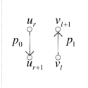
Figure 14: Two nodes $u_{r}$ and $v_{l}$ with two neighbors that are both the next node on the path

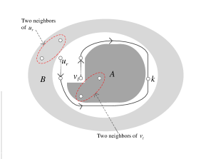
(a)

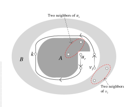
(b)

Figure 15: $p_{0}$ and $p_{1}$ merge at node $k$ to form a closed area $A$.

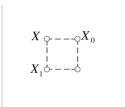
(a)

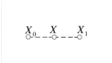
(b)

Figure 16: Possible relative positions for $X$, $X_{0}$ and $X_{1}$.

As a consequence, $g_{p_{0}}(i_{1})g_{p_{1}}(j_{1})$ is a term in $a_{S_{0}}(i_{1})a_{T_{1}}(j_{1})\oplus a_{S_{1}}(i_{1})a_{T_{0}}(j_{1})$ that is not equivalent to any other term. Thus, $g_{p_{0}}(i_{1})g_{p_{1}}(j_{1})$ contains a set of factors that is different from any other term.

We can represent $a_{S_{0}}(i_{1})a_{T_{1}}(j_{1})\oplus a_{S_{1}}(i_{1})a_{T_{0}}(j_{1})$ by

$$Q_{1}\oplus Q_{2}\oplus...\oplus Q_{L}$$ (56)

where each element in $\{Q_{j}\}_{j=1,2,...,L}$ is a product of two path coefficients, i.e.,

$$Q_{j}=g_{p}(i_{1})g_{p^{\prime}}(j_{1})$$

for some $p\in S_{0}$ and $p^{\prime}\in T_{1}$, or $p\in S_{1}$ and $p^{\prime}\in T_{0}$. An element in $\{Q_{j}\}_{j=1,2,...,L}$ is

$$Q_{j}=g_{p}(i_{1})g_{p^{\prime}}(j_{1})=\prod_{u\mbox{ is in }p}\alpha_{u}(t_{u})\prod_{v\mbox{ is in }p^{\prime}}\alpha_{v}(t_{v})$$

where $t_{u}$ and $t_{v}$ are the rounds node $u$ and $v$ are visited, respectively. Thus, $Q_{j}$ is a product of $R=i_{1}+j_{0}=i_{0}+j_{1}$ transmit coefficients. Without loss of generality, let $Q_{1}=g_{p_{0}}(i_{1})g_{p_{1}}(j_{1})$. Then $Q_{1}$ contains a set of distinct factors that is not exactly the same as that of any $Q_{j},2\leq j\leq L$. By Lemma 1, $a_{S_{0}}(i_{1})a_{T_{1}}(j_{1})\oplus a_{S_{1}}(i_{1})a_{T_{0}}(j_{1})\not\equiv 0$.

Therefore $a_{S_{0}}(i_{1})a_{T_{1}}(j_{1})\oplus a_{S_{1}}(i_{1})a_{T_{0}}(j_{1})\not\equiv 0$ when $i_{0}<i_{1}$, $j_{0}<j_{1}$ and $i_{1}-i_{0}=j_{1}-j_{0}$.∎

Lemma 1.

Consider a degree-$R$ multivariable polynomial $Q_{1}\oplus Q_{2}\oplus...\oplus Q_{L}$, where each of $Q_{i},1\leq i\leq L,$ is a product of $R\geq 1$ factors (variables), wherein the same factor can appear at most twice in each $Q_{i}$. Suppose that there is a $Q_{j},1\leq j\leq L,$ whose factors are all distinct and whose factors are not exactly the same as the factors of $Q_{i},1\leq i\leq L,i\neq j$ (i.e., there must be at least one factor in $Q_{j}$ that is not in $Q_{i}$). Then $Q_{1}\oplus Q_{2}\oplus...\oplus Q_{L}\not\equiv 0$.

Remark: This is an intuitively trivial lemma. It basically says that if there is a $Q_{j}$ that is pairwise distinct from any other $Q_{i},i\neq j$, then the overall polynomial cannot cancel out to zero algebraically. Here, we have not considered substituting the variables in the polynomial with specific values. Later in Lemma 2, we will consider assigning i.i.d. random values to each of the variables in the polynomial in the context of our random transmit coefficients.

Proof:

Without loss of generality, suppose that $j=1$ (i.e., $Q_{j}$ is $Q_{1}$). Also, without loss of generality, we assume if $Q_{i}=Q_{l}$ for $i,l\neq 1,i\neq l$, then they will be removed from $Q_{1}\oplus Q_{2}\oplus...\oplus Q_{L}$ so that $Q_{i}\neq Q_{l}$ in the remaining $Q_{1}\oplus Q_{2}\oplus...\oplus Q_{L}$. We write

$$Q_{1}=\prod_{m=1}^{R}r_{m},$$

where $r_{m}\neq r_{m^{\prime}}$ for $m\neq m^{\prime},1\leq m,m^{\prime}\leq R$.

First, consider the case of $R=1$. If $L=1$, then $Q_{1}\oplus Q_{2}\oplus...\oplus Q_{L}=Q_{1}=r_{1}\not\equiv 0$. For $L>1$, since $Q_{i}\neq Q_{l}$ for $i\neq l$ it is also clear that $Q_{1}\oplus Q_{2}\oplus...\oplus Q_{L}\not\equiv 0$, since all of $Q_{i}$ consist of one distinct variable.

Now, suppose that the lemma is true for $R=k$ for some $k\geq 1$, we will show that it is also true for $R=k+1$. We write

$$Q_{1}\oplus Q_{2}\oplus...\oplus Q_{L} =r_{1}(r_{2}...r_{k+1}\oplus\sum_{n}s_{n}^{(k)})\oplus\sum_{n}s_{n}^{(k+1)}$$

where $s_{n}^{(k)}$ and $s_{n}^{(k+1)}$ are products of $k$ and $k+1$ factors, respectively. Specifically, each of $s_{n}^{(k)}$ represents a $Q_{i}$ with factor $r_{1}$, and each of $s_{n}^{(k+1)}$ represents a $Q_{i}$ that does not have factor $r_{1}$. We know that $\nexists s_{n}^{(k)}$ such that $s_{n}^{(k)}=r_{2}r_{3}...r_{k+1}$, otherwise $\exists Q_{i}=r_{1}s_{n}^{(k)}$ such that $Q_{i}=Q_{1}$, contradicting our supposition that $Q_{1}$ contains a set of factors that is not the same as any of $Q_{i},2\leq i\leq L$. If $\sum_{n}s_{n}^{(k+1)}\equiv 0$, then

$$r_{1}(r_{2}...r_{k+1}\oplus\sum_{n}s_{n}^{(k)})\oplus\sum_{n}s_{n}^{(k+1)}\equiv 0$$

$$\Leftrightarrow r_{2}...r_{k+1}\oplus\sum_{n}s_{n}^{(k)}\equiv 0$$

which is impossible by the supposition that this lemma is true for $R=k$. If $\sum_{n}s_{n}^{(k+1)}\not\equiv 0$, it is trivially true that $r_{1}(r_{2}...r_{k+1}\oplus\sum_{n}s_{n}^{(k)})\not\equiv\sum_{n}s_{n}^{(k+1)}$, because $r_{1}$ does not appear on the RHS while it does on the LHS.

In conclusion, the lemma is true for any $R\geq 1$.∎

Lemma 2.

Consider a degree-$R$ multivariable polynomial $Q_{1}\oplus Q_{2}\oplus...\oplus Q_{L}$, where each of $Q_{i},1\leq i\leq L,$ is a product of $R\geq 1$ factors (variables), wherein the same factor can appear at most twice in each $Q_{i}$. Suppose that there is a $Q_{j},1\leq j\leq L,$ whose factors are all distinct and whose factors are not exactly the same as the factors of $Q_{i},1\leq i\leq L,i\neq j$ (i.e., there must be at least one factor in $Q_{j}$ that is not in $Q_{i}$). Further suppose that the factors (variables) in the polynomial $Q_{1}\oplus Q_{2}\oplus...\oplus Q_{L}$ are i.i.d. uniform random variables with values drawn from $GF(2^{s})\backslash\{0\}$. Then $\Pr\left(Q_{1}\oplus Q_{2}\oplus...\oplus Q_{L}=0\right)\leq R/(2^{s}-1)$.

Proof:

$Q_{1}\oplus Q_{2}\oplus...\oplus Q_{L}\not\equiv 0$ by Lemma 1. Without loss of generality, suppose that $j=1$ (i.e., $Q_{j}$ is $Q_{1}$). Also, without loss of generality, we assume if $Q_{i}=Q_{l}$ for $i,l\neq 1,i\neq l$, then they will be removed from $Q_{1}\oplus Q_{2}\oplus...\oplus Q_{L}$ so that $Q_{i}\neq Q_{l}$ in the remaining $Q_{1}\oplus Q_{2}\oplus...\oplus Q_{L}$. We write

$$Q_{1}=\prod_{m=1}^{R}r_{m},$$

where $r_{m}\neq r_{m^{\prime}}$ for $m\neq m^{\prime},1\leq m,m^{\prime}\leq R$.

First, consider the case of $R=1$.

$$\Pr\left(Q_{1}\oplus Q_{2}\oplus...\oplus Q_{L}=0\right)= \Pr\left(r_{1}=Q_{2}\oplus...\oplus Q_{L}\right)$$

$$\leq \frac{1}{2^{s}-1}.$$

Note that to arrive at the inequality above, if the realization of $Q_{2}\oplus...\oplus Q_{L}=0$, then $\Pr\left(r_{1}=0\right)=0$; if on the other hand $Q_{2}\oplus...\oplus Q_{L}\neq 0$, then $\Pr\left(r_{1}=Q_{2}\oplus...\oplus Q_{L}\right)=1/(2^{s}-1)$, regardless of what non-zero realization $Q_{2}\oplus...\oplus Q_{L}$ take.

Next, suppose that this lemma is true for $R=k$ for some $k\geq 1$, we want to show that it is also true for $R=k+1$. We write

$$Q_{1}\oplus Q_{2}\oplus...\oplus Q_{L}$$

$$= r_{1}...r_{k+1}\oplus Q_{2}\oplus...\oplus Q_{L}$$

$$= r_{1}^{2}\sum_{n}s_{n}^{(k-1)}\oplus r_{1}(r_{2}...r_{k+1}\oplus\sum_{n}s_{n}^{(k)})\oplus\sum_{n}s_{n}^{(k+1)}$$

where $s_{n}^{(k-1)}$, $s_{n}^{(k)}$ and $s_{n}^{(k+1)}$ are respectively products of $k-1$, $k$ and $k+1$ factors, all of whom are not $r_{1}$. We know that $\nexists s_{n}^{(k)}$ such that $s_{n}^{(k)}\equiv r_{2}r_{3}...r_{R}$, otherwise $\exists Q_{i}=r_{1}s_{n}^{(k)}$ such that $Q_{i}=Q_{1}$, contradicting our supposition that $Q_{1}$ contains a set of factors that is not the same as any $Q_{i},2\leq i\leq L$.

$r_{1}(r_{2}...r_{k+1}\oplus\sum_{n}s_{n}^{(k)})\not\equiv 0$ because $r_{2}...r_{k+1}\oplus\sum_{n}s_{n}^{(k)}\not\equiv 0$ by Lemma 1. There are four cases to be considered as follows:

1. $\sum_{n}s_{n}^{(k-1)}\equiv 0,\sum_{n}s_{n}^{(k+1)}\equiv 0$ (this is the case where $r_{1}$ appears once in all of $Q_{i}$):

$$\Pr\left(Q_{1}\oplus Q_{2}\oplus...\oplus Q_{L}=0\right)$$

$$= \Pr\left(r_{1}(r_{2}...r_{k+1}\oplus\sum_{n}s_{n}^{(k)})=0\right)$$

$$= \Pr\left(r_{2}...r_{k+1}\oplus\sum_{n}s_{n}^{(k)}=0\right)$$

$$\leq \frac{k}{2^{s}-1}$$

$$\leq \frac{k+1}{2^{s}-1}$$

by the supposition that this lemma is true for $R=k$,

2. $\sum_{n}s_{n}^{(k-1)}\equiv 0,\sum_{n}s_{n}^{(k+1)}\not\equiv 0$:

$$\Pr\left(Q_{1}\oplus Q_{2}\oplus...\oplus Q_{L}=0\right)$$

$$= \Pr\left(r_{1}(r_{2}...r_{k+1}\oplus\sum_{n}s_{n}^{(k)})\oplus\sum_{n}s_{n}^{(k+1)}=0\mid r_{2}...r_{k+1}\oplus\sum_{n}s_{n}^{(k)}=0\right)$$

$$\cdot\Pr\left(r_{2}...r_{k+1}\oplus\sum_{n}s_{n}^{(k)}=0\right)+$$

$$\Pr\left(r_{1}(r_{2}...r_{k+1}\oplus\sum_{n}s_{n}^{(k)})\oplus\sum_{n}s_{n}^{(k+1)}=0\mid r_{2}...r_{k+1}\oplus\sum_{n}s_{n}^{(k)}\neq 0\right)$$

$$\cdot\Pr\left(r_{2}...r_{k+1}\oplus\sum_{n}s_{n}^{(k)}\neq 0\right)$$

$$= \Pr\left(\sum_{n}s_{n}^{(k+1)}=0\right)\Pr\left(r_{2}...r_{k+1}\oplus\sum_{n}s_{n}^{(k)}=0\right)+$$

$$\Pr\left(r_{1}=\frac{\sum_{n}s_{n}^{(k+1)}}{r_{2}...r_{k+1}\oplus\sum_{n}s_{n}^{(k)}}\mid r_{2}...r_{k+1}\oplus\sum_{n}s_{n}^{(k)}\neq 0\right)$$

$$\cdot\Pr\left(r_{2}...r_{k+1}\oplus\sum_{n}s_{n}^{(k)}\neq 0\right)$$

$$\leq \Pr\left(r_{2}...r_{k+1}\oplus\sum_{n}s_{n}^{(k)}=0\right)+$$

$$\Pr\left(r_{1}=\frac{\sum_{n}s_{n}^{(k+1)}}{r_{2}...r_{k+1}\oplus\sum_{n}s_{n}^{(k)}}\mid r_{2}...r_{k+1}\oplus\sum_{n}s_{n}^{(k)}\neq 0\right).$$

Now,

$$\Pr\left(r_{2}...r_{k+1}\oplus\sum_{n}s_{n}^{(k)}=0\right)\leq\frac{k}{2^{s}-1}$$

by the supposition that this lemma is true for $R=k$. If $\sum_{n}s_{n}^{(k+1)}=0$, then

$$\Pr\left(r_{1}=\frac{\sum_{n}s_{n}^{(k+1)}}{r_{2}...r_{k+1}\oplus\sum_{n}s_{n}^{(k)}}\mid r_{2}...r_{k+1}\oplus\sum_{n}s_{n}^{(k)}\neq 0\right)$$

$$= \Pr\left(r_{1}=0\right)$$

$$= 0.$$

On the other hand, if $\sum_{n}s_{n}^{(k+1)}\neq 0$, then

$$\Pr\left(r_{1}=\frac{\sum_{n}s_{n}^{(k+1)}}{r_{2}...r_{k+1}\oplus\sum_{n}s_{n}^{(k)}}\mid r_{2}...r_{k+1}\oplus\sum_{n}s_{n}^{(k)}\neq 0\right)$$

$$= \frac{1}{2^{s}-1}$$

as $r_{1},...,r_{k+1}$ are i.i.d. uniform random variables with values drawn from $GF(2^{s})\backslash\{0\}$ and $r_{1}$ is not a factor in either $s_{n}^{(k)},\forall n$ or $s_{n}^{(k+1)},\forall n$. Thus,

$$\Pr\left(Q_{1}\oplus Q_{2}\oplus...\oplus Q_{L}=0\right)\leq \frac{k}{2^{s}-1}+\frac{1}{2^{s}-1}$$

$$= \frac{k+1}{2^{s}-1}.$$

3. $\sum_{n}s_{n}^{(k-1)}\not\equiv 0,\sum_{n}s_{n}^{(k+1)}\equiv 0$:

$$\Pr\left(Q_{1}\oplus Q_{2}\oplus...\oplus Q_{L}=0\right)$$

$$= \Pr\left(r_{1}^{2}\sum_{n}s_{n}^{(k-1)}\oplus r_{1}(r_{2}...r_{k+1}\oplus\sum_{n}s_{n}^{(k)})=0\right)$$

$$= \Pr\left(r_{1}\sum_{n}s_{n}^{(k-1)}\oplus(r_{2}...r_{k+1}\oplus\sum_{n}s_{n}^{(k)})=0\right)$$

$$= \Pr\left(r_{1}\sum_{n}s_{n}^{(k-1)}=0\mid r_{2}...r_{k+1}\oplus\sum_{n}s_{n}^{(k)}=0\right)$$

$$\cdot\Pr\left(r_{2}...r_{k+1}\oplus\sum_{n}s_{n}^{(k)}=0\right)+$$

$$\Pr\left(r_{1}\sum_{n}s_{n}^{(k-1)}\oplus(r_{2}...r_{k+1}\oplus\sum_{n}s_{n}^{(k)})=0\right.$$

$$\left.\mid r_{2}...r_{k+1}\oplus\sum_{n}s_{n}^{(k)}\neq 0\right)$$

$$\cdot\Pr\left(r_{2}...r_{k+1}\oplus\sum_{n}s_{n}^{(k)}\neq 0\right)$$

$$\leq \Pr\left(r_{2}...r_{k+1}\oplus\sum_{n}s_{n}^{(k)}=0\right)+$$

$$\Pr\left(r_{1}\sum_{n}s_{n}^{(k-1)}\oplus(r_{2}...r_{k+1}\oplus\sum_{n}s_{n}^{(k)})=0\right.$$

$$\left.\mid r_{2}...r_{k+1}\oplus\sum_{n}s_{n}^{(k)}\neq 0\right)$$

where

$$\Pr\left(r_{2}...r_{k+1}\oplus\sum_{n}s_{n}^{(k)}=0\right)\leq\frac{k}{2^{s}-1}$$

by the supposition that this lemma is true for $R=k$. If $\sum_{n}s_{n}^{(k-1)}=0$, then

$$\Pr\left(r_{1}\sum_{n}s_{n}^{(k-1)}\oplus(r_{2}...r_{k+1}\oplus\sum_{n}s_{n}^{(k)})=0\right.$$

$$\left.\mid r_{2}...r_{k+1}\oplus\sum_{n}s_{n}^{(k)}\neq 0\right)$$

$$= \Pr\left(r_{2}...r_{k+1}\oplus\sum_{n}s_{n}^{(k)}=0\mid r_{2}...r_{k+1}\oplus\sum_{n}s_{n}^{(k)}\neq 0\right)$$

$$= 0.$$

On the other hand, if $\sum_{n}s_{n}^{(k-1)}\neq 0$, then

$$\Pr\left(r_{1}\sum_{n}s_{n}^{(k-1)}\oplus(r_{2}...r_{k+1}\oplus\sum_{n}s_{n}^{(k)})=0\right.$$

$$\left.\mid r_{2}...r_{k+1}\oplus\sum_{n}s_{n}^{(k)}\neq 0\right)$$

$$= \Pr\left(r_{1}=\frac{r_{2}...r_{k+1}\oplus\sum_{n}s_{n}^{(k)}}{\sum_{n}s_{n}^{(k+1)}}\mid r_{2}...r_{k+1}\oplus\sum_{n}s_{n}^{(k)}\neq 0\right)$$

$$= \frac{1}{2^{s}-1}$$

as $r_{1},...,r_{k+1}$ are i.i.d. uniform random variables with values drawn from $GF(2^{s})\backslash\{0\}$ and $r_{1}$ is not a factor in either $s_{n}^{(k)},\forall n$ or $s_{n}^{(k+1)},\forall n$. Thus,

$$\Pr\left(Q_{1}\oplus Q_{2}\oplus...\oplus Q_{L}=0\right)\leq \frac{k}{2^{s}-1}+\frac{1}{2^{s}-1}$$

$$= \frac{k+1}{2^{s}-1}.$$

4. $\sum_{n}s_{n}^{(k-1)}\not\equiv 0,\sum_{n}s_{n}^{(k+1)}\not\equiv 0$: The equation

$$r_{1}^{2}\sum_{n}s_{n}^{(k-1)}\oplus r_{1}(r_{2}...r_{k+1}\oplus\sum_{n}s_{n}^{(k)})\oplus\sum_{n}s_{n}^{(k+1)}=0$$

is a second order polynomial with at most two solutions as far as $r_{1}$ is concerned. The probability for $r_{1}$ to be one of the two solutions is $2/(2^{s}-1)$. Thus,

$$\Pr\left(Q_{1}\oplus Q_{2}\oplus...\oplus Q_{L}=0\right)\leq\frac{2}{2^{s}-1}\leq\frac{k+1}{2^{s}-1}.$$

In conclusion, the lemma is true for any $R\geq 1$. ∎

-D Verification of Conjecture 1.

Consider the $7\times 5$ grid network in Fig. 9b. It can be transformed to the network in Fig. 11b, whose colored graph is shown in Fig. 12b. Table IV lists the two disjoint shortest paths for all non-virtual-source nodes.

TABLE IV: Two disjoint shortest paths for all non-virtual-source nodes in Fig. 11b.

Node #	Shortest path from $X_{0}$	Shortest path from $X_{1}$
2	1-2	31-30-29-4-3-2
3	1-2-3	31-30-29-4-3
4	1-2-3-4	31-30-29-4
5	1-2-7-6-5	31-30-29-4-5
6	1-2-7-6	31-30-29-4-5-6
6*	1-2-7-6-7*-6*	31-30-29-4-5-6*
7	1-2-7	31-30-29-4-5-6-7
7*	1-8-9-8*-7*	31-30-29-4-5-6*-7*
8	1-8	31-2-7-8*-9-8
8*	1-8-9-8*	31-2-7-8*
9	1-8-9	31-2-7-8*-7*-12-11-10
10	1-8-9-10	31-2-7-8*-7*-12-11-10
11	1-8-9-10-11	31-2-7-8*-7*-12-11
12	1-8-9-10-11-12	31-2-7-8*-7*-12
13	1-8-9-10-11-16-15-14-13	31-2-7-8*-7*-12-13
14	1-8-9-10-11-16-15-14	31-2-7-8*-7*-12-13-14
15	1-8-9-10-11-16-15	31-2-7-8*-7*-12-13-14-15
16	1-8-9-10-11-16	31-2-7-8*-7*-12-13-14-15-16
17	1-8-21-20-19-18-17	31-2-7-8*-9-10-17
18	1-8-21-20-19-18	31-2-7-8*-9-10-17-18
19	1-8-21-20-19	31-2-7-8*-9-10-17-18-19
20	1-8-21-20	31-2-7-8*-9-10-17-18-19-20
21	1-8-21	31-26-25-24-23-22-21
22	1-8-21-22	31-26-25-24-23-22
23	1-8-21-22-23	31-26-25-24-23
24	1-8-21-22-23-24	31-26-25-24
25	1-8-21-22-23-24-25	31-26-25
26	1-2-3-4-29-28-27-26	31-26
27	1-2-3-4-29-28-27	31-26-27
28	1-2-3-4-29-28	31-26-27-28
29	1-2-3-4-29	31-30-29
30	1-2-3-4-29-30	31-30

Consider the $10\times 9$ grid network in Fig. 18a. It can be transformed to the network in Fig. 18c, whose colored graph is shown in Fig. 18b. Table V and VI list the two disjoint shortest paths for all non-virtual-source nodes.

To verify the conjecture, we used a computer program to enumerate all shortest paths from a node to the two virtual sources. As the time needed to enumerate all shortest paths in a grid grows exponentially with the number of nodes, and due to the limit of time, we cannot thoroughly investigate large grid networks. According to our result, the conjecture at least applies to all grid networks not larger than $10\times 10$.

The conjecture does not apply directly to some grid networks with special source positions. For example, the conjecture does not apply to the $10\times 8$ grid network when the source is at one of the following positions: (1,1), (1,7), (2,1), (3,7), (4,1), (4,7), (5,1), (5,7), (6,7), (7,1), (8,1), (8,7). However, we can flip the Hamiltonian cycle horizontally (as shown in Fig. 17) to transform these positions to (1,6), (1,0), (2,6), (3,0), (4,6), (4,0), (5,6), (5,0), (6,0), (7,6), (8,6), (8,0), where the conjecture applies. We have verified that the conjecture applies to all networks not larger than $10\times 10$ if we allow flipping the Hamiltonian cycle.

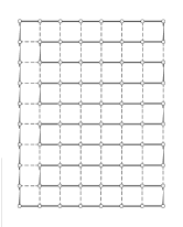
(a) Original Hamiltonian cycle

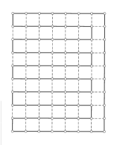
(b) Flipped Hamiltonian cycle

Figure 17: A $10\times 8$ grid network with the original and flipped Hamiltonian cycles.

TABLE V: Two disjoint shortest paths for non-virtual-source nodes 2-44 in Fig. 18c.

Node #	Shortest path from $X_{0}$	Shortest path from $X_{1}$
2	1-2	89-88-9-8-7-6-5-4-3-8
3	1-2-3	89-88-9-8-7-6-5-4-3
4	1-2-3-4	89-88-9-8-7-6-5-4
5	1-2-3-4-5	89-88-9-8-7-6-5
6	1-2-3-4-5-6	89-88-9-8-7-6
7	1-6-7	89-88-9-8-7
8	1-6-7-8	89-88-9-8
9	1-6-7-8-9	89-88-9
10	1-6-7-8-9-14-13-12-11-10	89-88-87-10
11	1-6-7-8-9-14-13-12-11	89-88-87-10-11
12	1-6-7-8-9-14-13-12	89-88-87-10-11-12
13	1-6-7-8-9-14-13	89-88-87-10-11-12-13
14	1-6-7-8-9-14	89-88-87-10-11-12-13-14
15	1-6-17-16-15	89-88-9-14-15
16	1-6-17-16	89-88-9-14-15-16
17	1-6-17	89-88-9-14-15-16-17
18	1-2-3-4-57-56-19-18	89-88-9-8-7-6-17-18
19	1-2-3-4-57-56-19	89-88-9-8-7-6-17-18-19
20	1-6-17-18-19-20	89-88-9-8-15-16-23-22-21-20
21	1-6-17-18-19-20-21	89-88-9-8-15-16-23-22-21
22	1-6-17-18-19-20-21-22	89-88-9-8-15-16-23
23	1-6-17-22-23	89-88-9-14-25-24-23
24	1-6-17-22-23	89-88-9-14-25-24
25	1-6-17-22-23-24-25	89-88-9-14-25
26	1-6-17-22-23-24-25-30-29-28-27-26	89-88-9-14-13-26
27	1-6-17-22-23-24-25-30-29-28-27	89-88-9-14-13-26-27
28	1-6-17-22-23-24-25-30-29-28	89-88-9-14-13-26-27-28
29	1-6-17-22-23-24-25-30-29	89-88-9-14-13-26-27-28-29
30	1-6-17-22-23-24-25-30	89-88-9-14-13-26-27-28-29-30
31	1-6-17-22-33-32-31	89-88-9-14-25-30-31
32	1-6-17-22-33-32	89-88-9-14-25-30-31-32
33	1-6-17-22-33	89-88-9-14-25-30-31-32-33
34	1-2-3-58-57-56-55-54-35-34	89-88-9-8-7-6-17-22-33-34
35	1-2-3-58-57-56-55-54-35	89-88-9-8-7-6-17-22-33-34-35
36	1-6-17-22-33-34-35-36	89-88-9-14-25-30-41-40-39-38-37-36
37	1-6-17-22-33-34-35-37	89-88-9-14-25-30-41-40-39-38-37
38	1-6-17-22-33-34-35-37-38	89-88-9-14-25-30-41-40-39-38
39	1-6-17-22-33-38-39	89-88-9-14-25-30-41-40-39
40	1-6-17-22-33-38-39-40	89-88-9-14-25-30-41-40
41	1-6-17-22-33-38-39-40-41	89-88-9-14-25-30-41
42	1-6-17-22-33-38-39-40-41-46-45-44-43-42	89-88-9-14-25-30-29-42
43	1-6-17-22-33-38-39-40-41-46-45-44-43	89-88-9-14-25-30-29-42-43
44	1-6-17-22-33-38-39-40-41-46-45-44	89-88-9-14-25-30-29-42-43-44

TABLE VI: Two disjoint shortest paths for non-virtual-source nodes 45-88 in Fig. 18c.

Node #	Shortest path from $X_{0}$	Shortest path from $X_{1}$
45	1-6-17-22-33-38-39-40-41-46-45	89-88-9-14-25-30-29-42-43-44-45
46	1-6-17-22-33-38-39-40-41-46	89-88-9-14-25-30-29-42-43-44-45-46
47	1-6-17-22-33-38-49-48-47	89-88-9-14-25-30-41-46-47
48	1-6-17-22-33-38-49-48	89-88-9-14-25-30-41-46-47-48
49	1-6-17-22-33-38-49	89-88-9-14-25-30-41-46-47-48-49
50	1-2-3-58-57-56-55-54-53-52-51-50	89-88-9-14-25-30-41-46-47-48-49-50
51	1-2-3-58-57-56-55-54-53-52-51	89-88-9-14-25-30-41-46-47-48-49-50-51
52	1-2-3-58-57-56-55-54-53-52	89-88-9-14-25-30-41-46-47-48-49-50-51-52
53	1-2-3-58-57-56-55-54-53	89-88-9-14-25-30-41-46-47-48-49-50-51-52-53
54	1-2-3-58-57-56-55-54	89-88-9-14-25-30-31-32-34-35-54
55	1-2-3-58-57-56-55	89-88-9-14-25-30-31-32-34-35-54-55
56	1-2-3-58-57-56	89-88-9-14-15-16-17-18-19-56
57	1-2-3-58-57	89-88-9-14-15-16-17-18-19-56-57
58	1-2-3-58	89-82-81-80-79-78-59-58
59	1-2-3-58-59	89-82-81-80-79-78-59
60	1-2-3-58-59-60	89-82-81-80-75-76-63-62-61-60
61	1-2-3-58-59-60-61	89-82-81-80-75-76-63-62-61
62	1-2-3-58-59-60-61-62	89-82-81-80-75-76-63-62
63	1-2-3-58-59-60-61-62-63	89-82-81-80-75-76-63
64	1-80-75-64	89-82-83-72-73-66-65-64
65	1-80-75-64-65	89-82-83-72-73-66-65
66	1-80-75-64-65-66	89-82-83-72-73-66
67	1-80-75-64-65-66-67	89-82-83-72-71-70-69-68-67
68	1-80-75-64-65-66-67-68	89-82-83-72-71-70-69-68
69	1-80-75-64-65-66-67-68-69	89-82-83-72-71-70-69
70	1-80-75-64-65-66-67-68-69-70	89-82-83-72-71-70
71	1-80-75-64-65-66-67-68-69-70-71	89-82-83-72-71
72	1-80-75-74-73-72	89-82-83-72
73	1-80-75-74-73	89-82-83-72-73
74	1-80-75-74	89-82-83-72-73-74
75	1-80-79-78-77-76-75	89-82-81-74-75
76	1-80-79-78-77-76	89-82-81-74-75-76
77	1-80-79-78-77	89-82-81-74-75-76-77
78	1-80-79-78	89-82-81-74-75-76-77-78
79	1-80-79	89-82-81-74-75-76-77-78-79
80	1-80	89-82-81-80
81	1-80-81	89-82-81
82	1-80-81-82	89-82
83	1-80-81-82-83	89-88-87-86-85-84-83
84	1-80-81-82-83-84	89-88-87-86-85-84
85	1-80-81-82-83-84-85	89-88-87-86-85
86	1-80-81-82-83-84-85-86	89-88-87-86
87	1-80-81-82-83-84-85-86-87	89-88-87
88	1-6-7-8-9-10-87-88	89-88

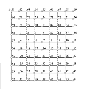
(a) Numbering

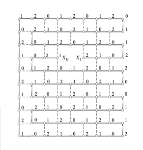
(b) Colored graph

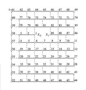
(c) Equivalent network

Figure 18: A $10\times 9$ network

References

- [1] S. Zhang, S. C. Liew, and P. P. Lam, “Hot topic: physical-layer network coding,” in Proc. 12th annual international conference on Mobile computing and networking. ACM, 2006, pp. 358–365.
- [2] B. Bollobas, “Graph theory, an introductory course,” 1979.
- [3] R. Ahlswede, N. Cai, S. Y. R. Li, and R. W. Yeung, “Network information flow,” IEEE Trans. Information Theory, vol. 46, no. 4, pp. 1204–1216, 2000.
- [4] S. Y. R. Li, R. W. Yeung, and N. Cai, “Linear network coding,” IEEE Trans. Information Theory, vol. 49, no. 2, pp. 371–381, 2003.
- [5] R. Koetter and M. Médard, “An algebraic approach to network coding,” IEEE/ACM Trans. Networking, vol. 11, no. 5, pp. 782–795, 2003.
- [6] S. Jaggi, P. Sanders, P. A. Chou, M. Effros, S. Egner, K. Jain, and L. M. Tolhuizen, “Polynomial time algorithms for multicast network code construction,” IEEE Trans. Information Theory, vol. 51, no. 6, pp. 1973–1982, 2005.
- [7] T. Ho, R. Koetter, M. Medard, D. R. Karger, and M. Effros, “The benefits of coding over routing in a randomized setting,” in Proc. 2003 IEEE International Symposium on Information Theory. IEEE, 2003.
- [8] T. Ho, M. Médard, R. Koetter, D. Karger, M. Effros, J. Shi, and B. Leong, “A random linear network coding approach to multicast,” IEEE Trans. Information Theory, vol. 52, no. 10, pp. 4413–4430, 2006.
- [9] S. Wang, Q. Song, X. Wang, and A. Jamalipour, “Distributed MAC protocol supporting physical-layer network coding,” IEEE Trans. Mobile Computing, vol. 12, no. 5, pp. 1023–1036, 2013.
- [10] H. Yomo and Y. Maeda, “Distributed MAC protocol for physical layer network coding,” in 14th International Symposium on Wireless Personal Multimedia Communications (WPMC). IEEE, 2011, pp. 1–5.
- [11] S. Zhang and S. C. Liew, “Channel coding and decoding in a relay system operated with physical-layer network coding,” IEEE Journal on Selected Areas in Communications, vol. 27, no. 5, pp. 788–796, 2009.
- [12] S. C. Liew, S. Zhang, and L. Lu, “Physical-layer network coding: Tutorial, survey, and beyond,” Physical Communication, vol. 6, no. 0, pp. 4 – 42, 2013.