Convergence of a data-driven time-frequency analysis method

Abstract

In a recent paper [12], Hou and Shi introduced a new adaptive data analysis method to analyze nonlinear and non-stationary data. The main idea is to look for the sparsest representation of multiscale data within the largest possible dictionary consisting of intrinsic mode functions of the form $\{a(t)\cos(\theta(t))\}$, where $a\in V(\theta)$, $V(\theta)$ consists of the functions smoother than $\cos(\theta(t))$ and $\theta^{\prime}\geq 0$. This problem was formulated as a nonlinear $L^{0}$ optimization problem and an iterative nonlinear matching pursuit method was proposed to solve this nonlinear optimization problem. In this paper, we prove the convergence of this nonlinear matching pursuit method under some sparsity assumption on the signal. We consider both well-resolved and sparse sampled signals. In the case without noise, we prove that our method gives exact recovery of the original signal.

1 Introduction

Developing a truly adaptive data analysis method is important for our understanding of many natural phenomena. Although a number of effective data analysis methods such as the Fourier transform or windowed Fourier transform have been developed, these methods use pre-determined basis and are mostly used to process linear and stationary data. Applications of these methods to nonlinear and nonstationary data tend to give many unphysical harmonic modes. To overcome these limitations of the traditional techniques, time-frequency analysis has been developed by representing a signal with a joint function of both time and frequency [10]. The recent advances of wavelet analysis have led to the development of several powerful wavelet-based time-frequency analysis techniques [14, 8, 20, 18]. But they still cannot remove the artificial harmonics completely and do not give satisfactory results for nonlinear signals.

Another important approach in the time-frequency analysis is to study instantaneous frequency of a signal. Some of the pioneering work in this area was due to Van der Pol [26] and Gabor [11], who introduced the so-called Analytic Signal (AS) method that uses the Hilbert transform to determine instantaneous frequency of a signal. However, this method works mostly for monocomponent signals in which the number of zero-crossings is equal to the number of local extrema [1]. There were other attempts to define instantaneous frequency such as the zero-crossing method [23, 24, 19] and the Wigner-Ville distribution method [1, 16, 22, 10, 15, 21]. Most of these methods suffer from various limitations. For example, the zero-crossing method cannot be applied to study a signal with multiple components and is sensitive to noise. On the other hand, the methods based on the Wigner-Ville distribution suffer from the interference between different components.

More substantial progress has been made recently with the introduction of the Empirical Mode Decomposition (EMD) method [13]. The EMD method decomposes a signal into a collection of intrinsic mode functions (IMFs) sequentially through a sifting process. On the other hand, since the EMD method relies on the information of local extrema of a signal, it is unstable to noise perturbation. Recently, an ensemble EMD method (EEMD) was proposed to make it more stable to noise perturbation [27]. But some fundamental issues remain unresolved.

Inspired by EMD/EEMD and the recently developed compressive sensing theory [6, 5, 9, 2], Hou and Shi proposed a data-driven time-frequency analysis method in a recent paper [12]. The main idea of this method is to look for the sparsest decomposition of a signal over the largest possible dictionary consisting of the intrinsic mode functions (IMFs). The dictionary is chosen to be:

$$\mathcal{D}=\left\{a\cos\theta:\;a\in V(\theta),\;\theta^{\prime}\in V(\theta),\mbox{and}\;\theta^{\prime}(t)\geq 0,\forall t\in\mathbb{R}\right\},$$ (1)

where $V(\theta)$ is a collection of all the functions that are smoother than $\cos\theta(t)$. In general, it is most effective to construct $V(\theta)$ as an overcomplete Fourier basis in the $\theta$-space. For periodic signals, we can simply choose $V(\theta)$ as the standard Fourier basis in the $\theta$-space. Then the problem can be reformulated as a nonlinear version of the $L^{0}$ minimization problem.

$$\begin{array}[]{rcc}\vspace{-2mm}P:&\mbox{Minimize}&M\\ \vspace{2mm}\hfil&{\scriptstyle(a_{k})_{1\leq k\leq M},(\theta_{k})_{1\leq k\leq M}}\\ &\mbox{Subject to:}&\left\{\begin{array}[]{l}f=\sum_{k=1}^{M}a_{k}\cos\theta_{k},\\ a_{k}\cos\theta_{k}\in\mathcal{D},\;\quad k=1,\cdots,M.\end{array}\right.\end{array}$$ (7)

The constraint $f=\sum_{k=1}^{M}a_{k}\cos\theta_{k}$ can be replaced by an inequality when the signal is polluted by noise. This kind of optimization problem is known to be very challenging to solve since both $a_{k}$ and $\theta_{k}$ are unknown. Inspired by matching pursuit [17, 25], Hou and Shi [12] proposed a nonlinear matching pursuit method to solve this nonlinear optimization problem. The basic idea is to decompose the signal sequentially into two parts, the mean plus a modulated oscillatory part with zero mean:

$$f=a_{0}+a_{1}\cos\theta,$$ (8)

where the mean $a_{0}$, the envelope $a_{1}$, and the phase function $\theta$ are all unknown. We call $a_{1}\cos\theta$ an Intrinsic Mode Function (IMF). After this decomposition is completed, we can treat $a_{0}$ as a new signal and repeat this process until the residual is small enough.

The objective of this paper is to analyze the convergence of the data-driven time-frequency analysis method proposed by Hou and Shi in [12] for periodic signals. We assume that the signal $f$ has a sparse representation over the Fourier basis in the $\theta$-space for some unknown $\theta$. The main objective of our data-driven time-frequency analysis is to design an iterative algorithm to find such $\theta$. With a given approximate phase function $\theta^{n}$, we solve a $l^{1}$ minimization problem to obtain the Fourier coefficients of $f$ in the $\theta^{n}$-space:

$$\min_{x}\|x\|_{1},\quad\mbox{subject to}\quad\Phi_{\theta^{n}}x=f,$$ (9)

where each column of matrix $\Phi_{\theta^{n}}$ is a Fourier basis in the $\theta^{n}$-space. We then use this coefficient $x$ to update $\theta^{n}$, and repeat this process until it converges.

When the signal has sufficiently well-resolved samples, the $l^{1}$ optimization problem (9) can be solved very efficiently by interpolation and Fast Fourier Transform (FFT). In this case, the constraint $\Phi_{\theta^{n}}x=f$ becomes a well-posed deterministic linear system provided that the coefficient matrix $\Phi_{\theta^{n}}$ is invertible. The linear optimization problem is then reduced to solving this linear system. Since the matrix $\Phi_{\theta^{n}}$ consists of the Fourier basis in the $\theta^{n}$-space, the corresponding linear system can be solved approximately by first interpolating $f$ to a uniform mesh in the $\theta^{n}$-space and then applying FFT. This gives rise to a very efficient algorithm with complexity of order $O(N\log(N))$, where $N$ is the number of sample points of the signal. Details of this algorithm will be given in Section 2.

Our first result is for well-resolved periodic signals of the form $f(t)=a_{0}(t)+a_{1}(t)\cos\theta(t)$. We ignore the interpolation error and assume that $f(t)$ is given for all $t\in[0,T]$. We further assume that the instantaneous frequency $\theta^{\prime}(t)$ has a sparse representation in the Fourier basis in the physical space given by $\left\{e^{i2k\pi t/T},\;\;|k|\leq M_{0}\right\}$, $a_{0}$ and $a_{1}$ have a sparse representation in the Fourier basis in the normalized $\theta$-space given by $\left\{e^{i2k\pi\bar{\theta}},\;\;|k|\leq M_{1}\right\}$, where $\bar{\theta}=\frac{\theta(t)-\theta(0)}{\theta(T)-\theta(0)}$ is the normalized phase function. Then we can prove that the iterative algorithm will converge to the exact solution under some mild scale separation assumption on the signal. More precisely, if the initial guess of $\theta$ satisfies

$$\|\mathcal{F}\left(\left(\theta^{0}-\theta\right)^{\prime}\right)\|_{1}\leq\pi M_{0}/2,\;$$ (10)

where $\mathcal{F}$ is the Fourier transform in the physical space, then there exists $\eta_{0}>0$ such that

$$\|\mathcal{F}\left(\left(\theta^{m+1}-\theta\right)^{\prime}\right)\|_{1}\leq\frac{1}{2}\left\|\mathcal{F}\left(\left(\theta^{m}-\theta\right)^{\prime}\right)\right\|_{1},$$ (11)

provided that $L\geq\eta_{0}$, where $\eta_{0}$ is a constant determined by $M_{0}$, $M_{1}$ and $L=\frac{\theta(T)-\theta(0)}{2\pi}$. We remark that $1/L$ is a measure of the smallest scale of the signal. The scales of $a_{0}$, $a_{1}$, and $\theta$ are measured by $1/M_{1}$ and $1/M_{0}$ respectively. The requirement $L\geq\eta_{0}$ is actually a mathematical formulation of the scale separation property.

The key idea of the proof is to estimate the decay rate of the coefficients over the Fourier basis in the $\theta^{n}$-space, where $\theta^{n}$ is the approximate phase function in each step. We show that the Fourier coefficients of the signal in the $\theta^{n}$-space have a very fast decay as long as that $\theta^{n}$ is a smooth function. Using this estimate, we can show that the error of the phase function in each step is a contraction and the iteration converges to the exact solution.

In many problems, a signal may not has an exact sparse representation. A more general setting is that the Fourier coefficients of $a_{0}$, $a_{1}$, and $\theta^{\prime}$ decay according to some power law as the wave number increases. We can prove that in this case, our method will converge to an approximate solution with an error determined by the truncated error of $a_{0}$, $a_{1}$ and $\theta^{\prime}$. The detailed analysis will be presented in Section 2.2.

For signals with sparse samples, we can also prove similar convergence results with an extra condition on the matrix $\Phi_{\theta^{n}}$. In this case, we need to use the $l^{1}$ minimization even with periodic signals. Suppose $S$ is the largest number such that $\delta_{3S}(\Phi_{\theta^{n}})+3\delta_{4S}(\Phi_{\theta^{n}})<2$. Under the same sparsity assumption on the instantaneous frequency, the mean and the envelope as before, we can prove that there exist $\eta_{L}>0,\;\eta_{S}>0$, such that

$$\|\mathcal{F}\left(\left(\theta^{m+1}-\theta\right)^{\prime}\right)\|_{1}\leq\frac{1}{2}\left\|\mathcal{F}\left(\left(\theta^{m}-\theta\right)^{\prime}\right)\right\|_{1},$$ (12)

provided that $L\geq\eta_{L}$ and $S\geq\eta_{S}$. Here the columns of the matrix consist of the Fourier basis in the $\theta^{n}$-space, $\delta_{S}(A)$ is the $S$-restricted isometry constant of matrix $A$ given in [3]. Further, we show that if the sample points $\{t_{j}\}_{j=1}^{N_{s}}$ are selected at random from a set of uniformly distributed points $\{t_{l}\}_{j=1}^{N_{f}}$, the condition $\delta_{3S}(\Phi_{\theta^{n}})+3\delta_{4S}(\Phi_{\theta^{n}})<2$ holds with an overwhelming probability provided that $S\leq CN_{s}/(\max(\overline{\theta}^{\prime}(\log N_{b})^{6})$ and $N_{f}\geq\max\{C\|\widehat{\overline{\theta}^{\prime}}\|_{1}N_{b},2M_{0}\}$, where $N_{s}$ is the number of the samples, $N_{b}$ is the number of the basis. If $M_{0}=0$, which implies that $\overline{\theta}^{\prime}=1$, then the above result is reduced to the well-known theorem for the standard Fourier basis in [7].

The rest of the paper is organized as follows. In Section 2, we establish the convergence and stability of our method for well-resolved signals. In Section 3, we propose an algorithm for signals with sparse samples and prove its convergence and stability. In Section 4, some numerical results are presented to demonstrate the performance of the algorithm and confirm the theoretical results. Some concluding remarks are made in Section 5.

2 Well resolved periodic signal

In this section, we will analyze the convergence and stability of the algorithm proposed in [12] for well-resolved signals. By well-resolved signals, we mean that that these signals are measured over a uniform grid and can be interpolated to any grid with very little loss of accuracy. In the analysis, we assume that the signal is periodic in the sample domain. Without loss of generality, we assume that the signal $f$ is periodic over $[0,1]$.

In order to make this paper self-contained, we state the algorithm proposed in [12]. The signal $f$ is given over a uniform grid $t_{j}=j/N$ for $j=0,...,N-1$.

• $\theta_{k}^{0}=\theta_{0},\;n=0$.

• Step 1: Interpolate $r_{k-1}$ from the uniform grid in the time domain to a uniform mesh in the $\theta_{k}^{n}$-coordinate to get $r_{\theta_{k}^{n}}^{k-1}$ and compute the Fourier transform $\widehat{r}_{\theta_{k}^{n}}^{k-1}$:

  $$r_{\theta_{k}^{n},\,j}^{k-1}=\mbox{Interpolate}\;\left(t_{i},r^{k-1},\theta_{k,\,j}^{n}\right),$$ (13)

  where $\theta_{k,\,j}^{n},\;j=0,\cdots,N-1$ are uniformly distributed in the $\theta_{k}^{n}$-coordinate,i.e. $\theta_{k,\,j}^{n}=2\pi L_{\theta_{k}^{n}}\;j/N$. Apply the Fourier transform to $r_{\theta_{k}^{n}}^{k-1}$ as follows:

  $$\widehat{r}_{\theta_{k}^{n}}^{k-1}(\omega)=\frac{1}{N}\sum_{j=1}^{N}r_{\theta^{n},\,j}^{k-1}e^{-i2\pi\omega\overline{\theta}_{k,\,j}^{n}},\quad\omega=-N/2+1,\cdots,N/2,$$ (14)

  where $\overline{\theta}_{k,\,j}^{n}=\frac{\theta_{k,\,j}^{n}-\theta_{k,\,0}^{n}}{2\pi L_{\theta_{k}^{n}}}$.

• Step 2: Apply a cutoff function to the Fourier Transform of $r_{\theta_{k}^{n}}^{k-1}$ to compute $a$ and $b$ on the mesh in the $\theta_{k}^{n}$-coordinate, denoted by $a_{\theta_{k}^{n}}$ and $b_{\theta_{k}^{n}}$:

  $$a_{\theta_{k}^{n}} = \mathcal{F}_{\theta_{k}^{n}}^{-1}\left[\left(\widehat{r}_{\theta_{k}^{n}}^{k-1}\left(\omega+L_{\theta_{k}^{n}}\right)+\widehat{r}_{\theta_{k}^{n}}^{k-1}\left(\omega-L_{\theta_{k}^{n}}\right)\right)\cdot\chi\left(\omega/L_{\theta_{k}^{n}}\right)\right],$$ (15)

  $$b_{\theta_{k}^{n}} = \mathcal{F}_{\theta_{k}^{n}}^{-1}\left[-i\cdot\left(\widehat{r}_{\theta_{k}^{n}}^{k-1}\left(\omega+L_{\theta_{k}^{n}}\right)-\widehat{r}_{\theta_{k}^{n}}^{k-1}\left(\omega-L_{\theta_{k}^{n}}\right)\right)\cdot\chi\left(\omega/L_{\theta_{k}^{n}}\right)\right],$$ (16)

  where $\mathcal{F}^{-1}$ is the inverse Fourier transform defined in the $\theta_{k}^{n}$ coordinate:

  $$\mathcal{F}_{\theta_{k}^{n}}^{-1}\left(\widehat{r}_{\theta_{k}^{n}}^{k-1}\right)=\frac{1}{N}\sum_{\omega=-N/2+1}^{N/2}\widehat{r}_{\theta_{k}^{n}}^{k-1}e^{i2\pi\omega\overline{\theta}_{k,\,j}^{n}},\quad j=0,\cdots,N-1,$$ (17)

  and $\chi$ is the cutoff function,

  $$\chi(\omega)=\left\{\begin{array}[]{cl}1,&-1/2<\omega<1/2,\\ 0,&\mbox{otherwise.}\end{array}\right.$$ (20)

• Step 3: Interpolate $a_{\theta_{k}^{n}}$ and $b_{\theta_{k}^{n}}$ back to the uniform mesh in the time domain:

  $$a_{k}^{n+1} = \mbox{Interpolate}\;\left(\theta_{k,\,j}^{n},a_{\theta_{k}^{n}},t_{i}\right),\quad i=0,\cdots,N-1,$$ (21)

  $$b_{k}^{n+1} = \mbox{Interpolate}\;\left(\theta_{k,\,j}^{n},b_{\theta_{k}^{n}},t_{i}\right),\quad i=0,\cdots,N-1,.$$ (22)

• Step 4: Update $\theta^{n}$ in the $t$-coordinate:

  $$\Delta\theta^{\prime}=P_{V_{M_{0}}}\left(\frac{d}{dt}\left(\arctan\left(\frac{b_{k}^{n+1}}{a_{k}^{n+1}}\right)\right)\right),\;\Delta\theta(t)=\int_{0}^{t}\Delta\theta^{\prime}(s)ds,\quad\theta^{n+1}=\theta^{n}+\beta\Delta\theta,$$

  where $\beta\in[0,1]$ is chosen to make sure that $\theta_{k}^{n+1}$ is monotonically increasing:

  $$\beta=\max\left\{\alpha\in[0,1]:\frac{d}{dt}\left(\theta_{k}^{n}+\alpha\Delta\theta\right)\geq 0\right\},$$ (23)

  and $P_{V_{M_{0}}}$ is the projection operator to the space $V_{M_{0}}=\mbox{span}\left\{e^{i2k\pi t/T},k=-M_{0},\cdots,0,\cdots,M_{0}\right\}$ and $M_{0}$ is chosen a priori.

• Step 5: If $\|\theta_{k}^{n+1}-\theta_{k}^{n}\|_{2}<\epsilon_{0}$, stop. Otherwise, set $n=n+1$ and go to Step 1.

In the previous paper [12], we demonstrated that this algorithm works very effectively for periodic signals and is stable to noise perturbation. In this paper, we will analyze its convergence and stability. Our main results can be summarized as follows. For periodic signals that have an exact sparsity structure, we can prove that the above algorithm will converge to the exact decomposition. For periodic signals that have an approximate sparsity structure, the above algorithm will give an approximate result withe accuracy determined by the truncated error of the signal. In the following two subsections, we will present these two results separately.

2.1 Exact recovery

In this section, we consider a periodic signal $f(t)$ that has the following decomposition:

$$f(t)=f_{0}(t)+f_{1}(t)\cos\theta(t),\;f_{1}(t)>0,\;\theta^{\prime}(t)>0,\;t\in[0,1],$$ (24)

where $f_{0},f_{1}$ and $\theta$ are the exact local mean, the envelope and the phase function that we want to recover from the signal.

First, we introduce some notations. Let $L=\frac{\theta(1)-\theta(0)}{2\pi}$ be the number of period of the signal which is a measurement of the scale of the signal. $\;\overline{\theta}=\frac{\theta-\theta(0)}{2\pi L}$ is the normalized phase function, which is used as a coordinate in our numerical method and analysis. $\widehat{f}_{0,\theta}(k),\widehat{f}_{1,\theta}(k)$ are the Fourier coefficients of $f_{0},f_{1}$ in the $\overline{\theta}$-coordinate, i.e.

$$\widehat{f}_{0,\theta}(k)=\int_{0}^{1}f_{0}\;e^{-i2\pi k\overline{\theta}}d\overline{\theta},\quad\widehat{f}_{1,\theta}(k)=\int_{0}^{1}f_{1}\;e^{-i2\pi k\overline{\theta}}d\overline{\theta},$$ (25)

We also use the notation $\mathcal{F}_{\theta}(\cdot)$ to represent the Fourier transform in the $\theta$-space and $\mathcal{F}(\cdot)$ to represent the Fourier transform in the original $t$-coordinate.

Now we can state the theorem as follows:

Theorem 2.1.

Assume that the instantaneous frequency $\theta^{\prime}$ is $M_{0}$-sparse over the Fourier basis in the physical space, i.e.

$$\theta^{\prime}\in V_{M_{0}}=\mbox{span}\left\{e^{i2k\pi t/T},k=-M_{0},\cdots,1,\cdots,M_{0}\right\}.$$ (26)

Further, we assume that the local mean $f_{0}$ and the envelope $f_{1}$ are $M_{1}$-sparse over the Fourier basis in the $\overline{\theta}$-space, i.e.

$$\widehat{f}_{0,\theta}(k)=\widehat{f}_{1,\theta}(k)=0,\quad\forall|k|>M_{1}.$$ (27)

If the initial guess of $\theta^{0}$ satisfies

$$\|\mathcal{F}\left(\left(\theta^{0}-\theta\right)^{\prime}\right)\|_{1}\leq\pi M_{0}/2,\;$$ (28)

then there exist $\eta_{0}>0$ such that

$$\|\mathcal{F}\left(\left(\theta^{m+1}-\theta\right)^{\prime}\right)\|_{1}\leq\frac{1}{2}\left\|\mathcal{F}\left(\left(\theta^{m}-\theta\right)^{\prime}\right)\right\|_{1},$$ (29)

provided that $L\geq\eta_{0}$.

Before giving the rigorous proof, we introduce some notations for the convenience of the representation. Let $\theta^{m}$ be the approximate phase function in the $m$th step, and $\Delta\theta^{m}=\theta-\theta^{m}$ be the error of the phase function in the current step. Let $\widetilde{a}^{m}$, $\widetilde{b}^{m}$ be the approximate envelope functions, which are obtained by using the algorithm in Step 3. Further, we define $a^{m}=f_{1}\cos\Delta\theta^{m}$, $b^{m}=f_{1}\sin\Delta\theta^{m}$, and $\Delta a^{m}=a^{m}-\widetilde{a}^{m}$ , $\Delta b^{m}=b^{m}-\widetilde{b}^{m}$. The quantities $a^{m}$ and $b^{m}$ can be considered as the “exact” envelope functions at the $m$th iteration since $\Delta\theta^{m}=\arctan\left(\frac{b^{m}}{a^{m}}\right)$. Thus, we would obtain the exact phase starting from $\theta^{m}$ in one iteration. In our analysis, we need to establish a relation among $\Delta a^{m}$, $\Delta b^{m}$ and $\Delta\theta^{m}$.

One key ingredient of the proof is to estimate the integral $\int_{0}^{1}e^{i2\pi(\omega\overline{\theta}-k\overline{\theta}^{m})}d\overline{\theta}^{m}$. Fortunately, for this type of integral, we have the following lemma.

Lemma 2.1.

Suppose $\phi^{\prime}(t)>0,\;t\in[0,1]$, $\phi(0)=0,\;\phi(1)=1$, and $\psi^{\prime},\phi^{\prime}\in V_{M_{0}}=\mbox{span}\left\{e^{i2k\pi t},k=-M_{0},\cdots,1,\cdots,M_{0}\right\}$. Then we have,

$$\left|\int_{0}^{1}e^{i\psi}e^{-i2\pi\omega\phi}d\phi\right|\leq\frac{P\left(\frac{\|\widehat{\phi^{\prime}}\|_{1}}{\min\phi^{\prime}},n\right)M_{0}^{n}}{|\omega|^{n}\left(\min\phi^{\prime}\right)^{n}}\sum_{j=1}^{n}(2\pi M_{0})^{-j}\|\widehat{\psi^{\prime}}\|_{1}^{j},$$ (30)

provided that $e^{i\psi}e^{-i2\pi\omega\phi}$ is a periodic function. Here $P(x,n)$ is a $(n-1)$th order polynomial of $x$ and the coefficients also depend on $n$.

Remark 2.1.

Regarding the polynomial $P(x,n)$, we can get an explicit expression for small $n$. For example, when $n=2$, we have

$$\left|\frac{d^{2}}{d\phi^{2}}e^{i\psi}\right| = \left|i\left(\frac{\psi^{\prime\prime}}{\phi^{\prime 2}}-\frac{\psi^{\prime}\phi^{\prime\prime}}{\phi^{\prime 3}}+i\frac{\psi^{\prime 2}}{\phi^{\prime 2}}\right)e^{i\psi}\right|\leq\left|\frac{\psi^{\prime\prime}}{\phi^{\prime 2}}\right|+\left|\frac{\psi^{\prime}\phi^{\prime\prime}}{\phi^{\prime 3}}\right|+\left|\frac{\psi^{\prime 2}}{\phi^{\prime 2}}\right|$$ (31)

$$\leq \frac{\max|\psi^{\prime\prime}|}{\left(\min\phi^{\prime}\right)^{2}}+\frac{\max|\psi^{\prime}|\max|\phi^{\prime\prime}|}{\left(\min\phi^{\prime}\right)^{3}}+\frac{\left(\max|\psi^{\prime}|\right)^{2}}{\left(\min\phi^{\prime}\right)^{2}}$$

$$\leq \frac{1}{\left(\min\phi^{\prime}\right)^{2}}\left[\left(1+\frac{\|\widehat{\phi^{\prime}}\|_{1}}{\min\phi^{\prime}}\right)2\pi M_{0}\|\widehat{\psi^{\prime}}\|_{1}+\|\widehat{\psi^{\prime}}\|_{1}^{2}\right],$$

where we have used $\Delta\theta,\overline{\theta}\in V_{M_{0}}$ in deriving the last inequality. Then, we have $P(x,2)=x+1$. Similarly, we can also get $P(x,3)=3x^{2}+4x+3$.

Remark 2.2.

Lemma 2.1 is valid for any $n\in\mathbb{N}$. The integral that we would like to estimate in Lemma 2.1 is actually the Fourier transform of $e^{i\psi}$. Since $\psi$ is a smooth function, we expect that the Fourier transform of $e^{i\psi}$ has a rapid decay for $|\omega|$ large. In Lemma 2.1, we give a more delicate decay estimate of the Fourier transform of $e^{i\psi}$. Such estimate is required in our proof of Theorem 2.1.

Proof.

Using integration by parts, then we have

$$\left|\int_{0}^{1}e^{i\psi}e^{-i2\pi\omega\phi}d\phi\right|=\frac{1}{|2\pi\omega|^{n}}\left|\int_{0}^{1}\frac{d^{n}(e^{i\psi})}{d\phi^{n}}e^{-i2\pi\omega\phi}d\phi\right|\leq\frac{1}{|2\pi\omega|^{n}}\max_{t\in[0,1]}\left|\frac{d^{n}(e^{i\psi})}{d\phi^{n}}\right|.$$

Since $e^{i\psi}e^{-i2\pi\omega\phi}$ is periodic, there is no contribution from the boundary terms when performing integration by parts. Using the fact that, $\psi^{\prime},\phi^{\prime}\in V_{M_{0}}$ and $\forall g\in V_{M_{0}}$, we obtain

$$\max_{t}|g^{(n)}(t)| \leq \sum_{k}|(2\pi k)^{n-1}\widehat{g^{\prime}}(k)|\leq(2\pi M_{0})^{n-1}\sum_{k}|\widehat{g^{\prime}}(k)|=(2\pi M_{0})^{n-1}\|\widehat{g^{\prime}}\|_{1}.$$ (32)

Direct calculations give

$$\left|\frac{d^{n}(e^{i\psi})}{d\phi^{n}}\right|\leq\frac{P\left(\frac{\|\widehat{\phi^{\prime}}\|_{1}}{\min\phi^{\prime}},n\right)}{\left(\min\phi^{\prime}\right)^{n}}\sum_{j=1}^{n}(2\pi M_{0})^{n-j}\|\widehat{\psi^{\prime}}\|_{1}^{j}.$$ (33)

Thus, we get

$$\left|\int_{0}^{1}e^{i\psi}e^{-i2\pi\omega\phi}d\phi\right| \leq \frac{P\left(\frac{\|\widehat{\phi^{\prime}}\|_{1}}{\min\phi^{\prime}},n\right)M_{0}^{n}}{|\omega|^{n}\left(\min\phi^{\prime}\right)^{n}}\sum_{j=1}^{n}(2\pi M_{0})^{-j}\|\widehat{\psi^{\prime}}\|_{1}^{j}.$$ (34)

This proves Lemma 2.1. ∎

Now we are ready to prove Theorem 2.1.

Proof.

of Theorem 2.1

First, we need to establish the relation between $\Delta\theta^{m+1}$ and $\Delta a^{m}$, $\Delta b^{m}$.

Recall that $\Delta\theta^{m}=\arctan\left(\frac{b^{m}}{a^{m}}\right)$. Thus, we have $\widetilde{\Delta\theta}=\Delta\theta^{m}-\arctan\left(\frac{\widetilde{b}^{m}}{\widetilde{a}^{m}}\right)=\arctan\left(\frac{b^{m}}{a^{m}}\right)-\arctan\left(\frac{\widetilde{b}^{m}}{\widetilde{a}^{m}}\right)$. Using the differential mean value theorem, we know that there exists $\xi\in[0,1]$, such that

$$\left|\widetilde{\Delta\theta}\right| = \left|\arctan\left(\frac{b^{m}}{a^{m}}\right)-\arctan\left(\frac{\widetilde{b}^{m}}{\widetilde{a}^{m}}\right)\right|=\left|\frac{(a^{m}+\xi\Delta a^{m})\Delta b^{m}-(b^{m}+\xi\Delta b^{m})\Delta a^{m}}{(a^{m}+\xi\Delta a^{m})^{2}+(b^{m}+\xi\Delta b^{m})^{2}}\right|$$ (35)

$$\leq \frac{(|a^{m}|+|\Delta a^{m}|)|\Delta b^{m}|+(|b^{m}|+|\Delta b^{m}|)|\Delta a^{m}|}{((a^{m})^{2}+(b^{m})^{2})/2-((\Delta a^{m})^{2}+(\Delta b^{m})^{2})}$$

$$\leq D_{1}|\Delta a^{m}|+D_{2}|\Delta b^{m}|,$$

where

$$D_{1}=\max_{t}\left\{\frac{f_{1}+|\Delta b^{m}|}{f_{1}^{2}/2-((\Delta a^{m})^{2}+(\Delta b^{m})^{2})}\right\},\;\displaystyle D_{2}=\max_{t}\left\{\frac{f_{1}+|\Delta a^{m}|}{f_{1}^{2}/2-((\Delta a^{m})^{2}+(\Delta b^{m})^{2})}\right\},\quad$$ (36)

and we have used the relations that $f_{1}^{2}=(a^{m})^{2}+(b^{m})^{2}$ and $|a^{m}|,|b^{m}|\leq f_{1}$.

In the algorithm, there is another smooth process when updating $\theta$, which gives the following result for $\Delta\theta^{m+1}$,

$$\Delta\theta^{m+1}=2\pi\Delta L^{m+1}t+\widetilde{\Delta\theta}_{p,M_{0}},$$ (37)

where $\widetilde{\Delta\theta}_{p,M_{0}}=P_{V_{M_{0}}}\left(\widetilde{\Delta\theta}_{p}\right)$ is the projection of $\widetilde{\Delta\theta}_{p}$ over the space $V_{M_{0}}$, $\widetilde{\Delta\theta}_{p}$ and $2\pi\Delta L^{m+1}t$ are the periodic part and the linear part of $\widetilde{\Delta\theta}$ respectively:

$$\widetilde{\Delta\theta}=2\pi\Delta L^{m+1}t+\widetilde{\Delta\theta}_{p}.$$ (38)

Using (37), we can estimate $(\Delta\theta^{m+1})^{\prime}$ as follows,

$$\left\|\mathcal{F}\left((\Delta\theta^{m+1})^{\prime}\right)\right\|_{1}\leq 2\pi\Delta L^{m+1}+\left\|\widehat{\widetilde{\Delta\theta}^{\prime}}_{p,M_{0}}\right\|_{1}\leq 2\pi\Delta L+M_{0}\left\|\widehat{\widetilde{\Delta\theta}}_{p,M_{0}}\right\|_{1}$$ (39)

$$\leq 2\|\widetilde{\Delta\theta}\|_{\infty}+M_{0}^{2}\left\|\widetilde{\Delta\theta}_{p}\right\|_{\infty}\leq(3M_{0}^{2}+2)\|\widetilde{\Delta\theta}\|_{\infty}.$$

where we have used the fact that

$$2\pi|\Delta L^{m+1}| = |\widetilde{\Delta\theta}(1)-\widetilde{\Delta\theta}(0)|\leq 2\|\widetilde{\Delta\theta}\|_{\infty},$$ (40)

$$\left\|\widetilde{\Delta\theta}_{p}\right\|_{\infty} = \left\|\widetilde{\Delta\theta}\right\|_{\infty}+2\pi\Delta L\leq 3\left\|\widetilde{\Delta\theta}\right\|_{\infty}.$$ (41)

Combining (39) with (35), we get

$$\left\|\mathcal{F}\left((\Delta\theta^{m+1})^{\prime}\right)\right\|_{1}\leq(3M_{0}^{2}+2)\left(D_{1}\|\Delta a^{m}\|_{\infty}+D_{2}\|\Delta b^{m}\|_{\infty}\right).$$ (42)

Next, we will establish the relation among $\Delta a^{m}$, $\Delta b^{m}$ and $\Delta\theta^{m}$. This can be done by estimating the Fourier coefficients of $\overline{a}^{m}$, $\overline{b}^{m}$ in the $\theta^{m}$-space.

In Appendix A, we derive the following estimates of $\Delta a^{m}$ and $\Delta b^{m}$ (see (151), (152)),

$$|\Delta a^{m}|\leq 2\sum_{\frac{1}{2}L^{m}<k<\frac{3}{2}L^{m}}\left|\widehat{f}_{0,\theta^{m}}(k)\right|+\sum_{\frac{3}{2}L^{m}<k<\frac{5}{2}L^{m}}\left(\left|\widehat{a}_{\theta^{m}}(k)\right|+\left|\widehat{b}_{\theta^{m}}(k)\right|\right)+\sum_{|k|>\frac{L^{m}}{2}}\left|\widehat{a}_{\theta^{m}}(k)\right|,\quad$$ (43)

$$|\Delta b^{m}|\leq 2\sum_{\frac{1}{2}L^{m}<k<\frac{3}{2}L^{m}}\left|\widehat{f}_{0,\theta^{m}}(k)\right|+\sum_{\frac{3}{2}L^{m}<k<\frac{5}{2}L^{m}}\left(\left|\widehat{a}_{\theta^{m}}(k)\right|+\left|\widehat{b}_{\theta^{m}}(k)\right|\right)+\sum_{|k|>\frac{L^{m}}{2}}\left|\widehat{b}_{\theta^{m}}(k)\right|,\quad$$ (44)

where $\widehat{f}_{0,\theta^{m}}$, $\widehat{a}^{m}_{\theta^{m}}$ and $\widehat{b}^{m}_{\theta^{m}}$ are the Fourier transform of $f_{0}$, $a^{m}$ and $b^{m}$ in the $\theta^{m}$-space.

To obtain the desired estimates, we need to use Lemma 2.1 to estimate the Fourier coefficients of $f_{0},\;a^{m},b^{m}$ in the $\theta^{m}$-space. In an effort to make the proof concise and easy to follow, we defer the derivation of the estimates (45), (46) and (47) to Appendix B. The main results of Appendix B are summarized as follows. As long as $\gamma=\frac{\|\mathcal{F}[(\Delta\theta^{m})^{\prime}]\|_{1}}{2\pi M_{0}}\leq 1/4$, we have

$$|\widehat{f}_{0,\theta^{m}}(\omega)| \leq C_{0}Q\left(\frac{|\omega|}{2}\right)^{-n}M_{0}^{n}M_{1}\gamma,\quad\forall|\omega|>L/2$$ (45)

$$|\widehat{a}^{m}_{\theta^{m}}(\omega)| \leq 4C_{0}Q\left(\frac{|\omega|}{2}\right)^{-n}M_{0}^{n}(2M_{1}+1)\gamma,\quad\forall|\omega|\geq L/2.$$ (46)

$$|\widehat{b}^{m}_{\theta^{m}}(\omega)| \leq 4C_{0}Q\left(\frac{|\omega|}{2}\right)^{-n}M_{0}^{n}(2M_{1}+1)\gamma,\quad\forall|\omega|\geq L/2.$$ (47)

where

$$Q=\frac{P\left(z,n\right)}{\left(\min(\overline{\theta}^{m})^{\prime}\right)^{n}},\quad z=\frac{\|\mathcal{F}[(\overline{\theta}^{m})^{\prime}]\|_{1}}{\min(\overline{\theta}^{m})^{\prime}},\quad\gamma=\frac{\|\mathcal{F}[(\Delta\theta^{m})^{\prime}]\|_{1}}{2\pi M_{0}}.$$ (48)

Using (43)-(47) and the fact that $\sum_{k=1}^{\infty}k^{-n}$ converges as long as $n\geq 2$, we conclude that

$$|\Delta a^{m}| \leq \Gamma_{0}Q(\alpha L)^{-n+1}\gamma,$$ (49)

$$|\Delta b^{m}| \leq \Gamma_{0}Q(\alpha L)^{-n+1}\gamma,$$ (50)

where $\Gamma_{0}$ is a constant that depends on $M_{0},M_{1}$ and $n$. It follows from (42), (48), (49) and (50) that

$$\left\|\mathcal{F}\left((\Delta\theta^{m+1})^{\prime}\right)\right\|_{1} \leq \Gamma_{1}(D_{1}+D_{2})Q(\alpha L)^{-n+1}\left\|\mathcal{F}\left((\Delta\theta^{m})^{\prime}\right)\right\|_{1},$$ (51)

where $\Gamma_{1}$ is a constant that depends on $M_{0},M_{1}$ and $n$.

To complete the proof, we need to show that there exists a constant $\eta_{0}>0$ which does not change in the iterative process, such that $\widetilde{\beta}=\Gamma_{1}(D_{1}+D_{2})Q(\alpha L)^{-n+1}\leq 1/2$ provided that $L\geq\eta_{0}$. This seems to be trivial, simply choosing $\eta_{0}=\frac{1}{\alpha}\left(2\Gamma_{1}(D_{1}+D_{2})Q\right)^{1/(n-1)}$ would make $\widetilde{\beta}\leq 1/2$ provided that $L\geq\eta_{0}$. The problem is that $D_{1},D_{2},Q,\alpha$ vary during the iteration. We need to show that they are uniformly bounded during the iteration.

It is relatively easy to show that $\alpha$ is bounded,

$$|1-\alpha|=\left|1-\frac{\theta^{m}(1)-\theta^{m}(0)}{\theta(1)-\theta(0)}\right|=\left|\frac{\Delta\theta^{m}(1)-\Delta\theta^{m}(0)}{2\pi L}\right|\leq\frac{\|(\Delta\theta^{m})^{\prime}\|_{\infty}}{2\pi L}\leq\|\frac{\mathcal{F}[(\Delta\theta^{m})^{\prime}]\|_{1}}{2\pi L}\leq\frac{M_{0}}{4L},$$

which implies that $7/8\leq\alpha\leq 9/8$, provided that $L\geq 2M_{0}$ and $\gamma\leq 1/4$.

It is more involved to show that $Q$ is bounded. We need to first estimate $|(\overline{\theta}^{m})^{\prime}|$ and $\|\mathcal{F}[(\overline{\theta}^{m})^{\prime}]\|_{1}$,

$$|(\overline{\theta}^{m})^{\prime}| = |\overline{\theta}^{\prime}-(\Delta\theta^{m})^{\prime}/(2\pi L^{m})|\geq\frac{1}{\alpha}\left(\overline{\theta}^{\prime}-\|\mathcal{F}[(\Delta\theta^{m})^{\prime}]\|_{1}/(2\pi L)\right)\geq\frac{8}{9}\left(\overline{\theta}^{\prime}-\frac{M_{0}}{4L}\right),$$ (52)

and

$$\|\mathcal{F}[(\overline{\theta}^{m})^{\prime}]\|_{1} = \frac{1}{\alpha}\|\widehat{\overline{\theta}^{\prime}}-\mathcal{F}[(\Delta\theta^{m})^{\prime}]/(2\pi L)\|_{1}\leq\frac{1}{\alpha}\left(\|\widehat{\overline{\theta}^{\prime}}\|_{1}+\|\mathcal{F}[(\Delta\theta^{m})^{\prime}]\|_{1}/(2\pi L)\right)$$ (53)

$$\leq \frac{8}{7}\left(\|\widehat{\overline{\theta}^{\prime}}\|_{1}+M_{0}/(4L)\right),$$

where we have used the assumption that $\gamma\leq\frac{1}{4}$. If $L$ satisfies the following condition,

$$\frac{M_{0}}{L}\leq 2\min(\overline{\theta}^{\prime}),$$ (54)

then we can get

$$|(\overline{\theta}^{m})^{\prime}|\geq\frac{4}{9}\overline{\theta}^{\prime},\quad\|\mathcal{F}[(\overline{\theta}^{m})^{\prime}]\|_{1}\leq\frac{12}{7}\|\widehat{\overline{\theta}^{\prime}}\|_{1},$$ (55)

where we have used the fact that $\min(\overline{\theta}^{\prime})\leq\max(\overline{\theta}^{\prime})\leq\|\widehat{\overline{\theta}^{\prime}}\|_{1}$. It follows from (55) that the term $z$ defined in (48) is uniformly bounded,

$$z\leq z_{0},$$ (56)

where $z_{0}$ is a constant depending on $\overline{\theta}^{\prime}$.

Based on the above estimation of $z$, the term $Q$ in (48) can be bounded by a constant,

$$Q=\frac{P\left(z,n\right)}{\left(\min(\overline{\theta}^{m})^{\prime}\right)^{n}}\leq\left(\frac{9}{4}\right)^{n}\frac{P\left(z_{0},n\right)}{\left(\min\overline{\theta}^{\prime}\right)^{n}}=Q_{0},$$ (57)

where $Q_{0}$ is a constant that depends on $\overline{\theta}^{\prime}$ and $n$.

We now proceed to bound $D_{1}$ and $D_{2}$. Note that if $|\Delta a^{m}|,|\Delta b^{m}|\leq\frac{\sqrt{2}}{4}\min f_{1}$, we can bound $D_{1}$ as follows:

$$D_{1} = \max\left\{\frac{|b^{m}|+|\Delta b^{m}|}{((a^{m})^{2}+(b^{m})^{2})/2-((\Delta a^{m})^{2}+(\Delta b^{m})^{2})}\right\}$$ (58)

$$\leq \max\frac{|f_{1}|+|\Delta b^{m}|}{(f_{1})^{2}/2-((\Delta a^{m})^{2}+(\Delta b^{m})^{2})}$$

$$\leq \frac{4+\sqrt{2}}{\min f_{1}}=E_{0}.$$

Similarly, we can show that $D_{2}\leq E_{0}$.

It is not difficult to see that the condition $|\Delta a^{m}|,|\Delta b^{m}|\leq\frac{\sqrt{2}}{4}\min f_{1}$ is valid if $L$ satisfies

$$\Gamma_{0}Q_{0}(7L/8)^{-n+1}\leq\sqrt{2}\min f_{1},$$ (59)

since we have

$$|\Delta a| \leq \Gamma_{0}Q(\alpha L)^{-n+1}\gamma\leq\frac{1}{4}\Gamma_{0}Q_{0}(7L/8)^{-n+1},$$ (60)

$$|\Delta b| \leq \Gamma_{0}Q(\alpha L)^{-n+1}\gamma\leq\frac{1}{4}\Gamma_{0}Q_{0}(7L/8)^{-n+1},$$ (61)

where we have used $\alpha\geq 7/8$, $Q\leq Q_{0}$, the assumption $\gamma\leq\frac{1}{4}$ and the estimates (43), (44).

Finally, we derive the following estimate for the error of the instantaneous frequency,

$$\left\|\mathcal{F}\left((\Delta\theta^{m+1})^{\prime}\right)\right\|_{1}\leq\beta\left\|\mathcal{F}\left((\Delta\theta^{m})^{\prime}\right)\right\|_{1},$$ (62)

where $\beta=\Gamma_{1}E_{0}Q_{0}(7L/8)^{-n+1}$, $\Gamma_{1}$ is a constant depends on $M_{0},M_{1},n$, $E_{0}$ depends on $\min f_{1}$, and $Q_{0}$ depends on $\overline{\theta}^{\prime}$ and $n$.

Now, we prove that if $\gamma=\frac{\|\mathcal{F}[(\Delta\theta^{m})^{\prime}]\|_{1}}{2\pi M_{0}}\leq\frac{1}{4}$, then we have

$$\left\|\mathcal{F}\left((\Delta\theta^{m+1})^{\prime}\right)\right\|_{1}\leq\frac{1}{2}\left\|\mathcal{F}\left((\Delta\theta^{m})^{\prime}\right)\right\|_{1},$$ (63)

as long as $L$ satisfies the following conditions

$$L\geq 4M_{1},\quad\frac{M_{0}}{L} \leq \min\left\{\frac{1}{2},2\min(\overline{\theta}^{\prime})\right\},$$ (64)

$$\Gamma_{0}Q_{0}(7L/8)^{-n+1} \leq \sqrt{2}\min f_{1},$$ (65)

$$\Gamma_{1}E_{0}Q_{0}(7L/8)^{n-1} \leq \frac{1}{2}.$$ (66)

It is obvious that there exist $\eta_{0}>0$, such that conditions (64)-(66) are satisfied provided that $L\geq\eta_{0}$. Here $\eta_{0}$ is determined by $M_{0},M_{1},\overline{\theta}^{\prime},\min f_{1}$ and $n$ which does not change during the iteration process.

By induction, it is easy to show that if initially

$$\frac{\|\mathcal{F}[(\theta^{0}-\theta)^{\prime}]\|_{1}}{2\pi M_{0}}\leq\frac{1}{4},$$

then there exists $\eta_{0}>0$ which is determined by $M_{0},M_{1},\overline{\theta}^{\prime},\min f_{1}$ and $n$, such that

$$\left\|\mathcal{F}\left((\Delta\theta^{m+1})^{\prime}\right)\right\|_{1}\leq\frac{1}{2}\left\|\mathcal{F}\left((\Delta\theta^{m})^{\prime}\right)\right\|_{1},$$ (67)

as long as $L\geq\eta_{0}$. This completes the proof of Theorem 2.1. ∎

Remark 2.3.

The above proof is valid for any $n\geq 2$. Note that $\eta_{0}$ depends on $n$. Theoretically, there exists an optimal choice of $n$ to make $\eta_{0}$ the smallest. By carefully tracking the constants in the proof, we can show that as $n$ going to $+\infty$, $\eta_{0}$ tends to $\delta C(n)^{1/(n-1)}M_{0}$, where $\delta$ is a constant independent on $n$, and $C(n)$ is the maximum of the coefficients of polynomial $P(x,n)$ appears in Lemma 2.1. We conjecture that $C(n)^{1/(n-1)}$ is bounded for $n\geq 2$. If this is the case, then $\eta_{0}$ is proportional to $M_{0}$.

Remark 2.4.

Classical time-frequency analysis methods, such as the windowed Fourier transform or wavelet transform, in general cannot extract the instantaneous frequency exactly for any signal due to the uncertainty principle. For a single linear chirp signal without amplitude modulation, the Wigner-Ville distribution can extract the exact instantaneous frequency, but it fails if the signal consists of several components. Theorem 2.1 shows that our data-driven time-frequency analysis method has the capability to recover the exact instantaneous frequency for a much larger range of signals.

2.2 Approximate recovery

If the signal does not have an exact sparsity structure in the $\theta$-space as required in Theorem 2.1, our method cannot reproduce the exact decomposition. But the analysis in this subsection shows that we can still get an approximate result and the accuracy is determined by the truncated error of the signal. The main result is stated below.

Theorem 2.2.

Assume that the instantaneous frequency $\theta^{\prime}$, has a sparse representation, i.e. there exists $M_{0}$, such that

$$\theta^{\prime}(t)\in V_{M_{0}}=\mbox{span}\left\{e^{i2k\pi t/T},k=-M_{0},\cdots,1,\cdots,M_{0}\right\}.$$ (68)

and the Fourier coefficients of the local mean $f_{0}$ and the envelope $f_{1}$ in the $\overline{\theta}$-space have a fast decay, i.e. there exists $C_{0}>0,\;p\geq 4$ such that

$$|\widehat{f}_{0,\theta}(k)|\leq C_{0}|k|^{-p},\quad|\widehat{f}_{1,\theta}(k)|\leq C_{0}|k|^{-p}.$$ (69)

Then, there exists $\eta_{0}>4$ such that if $L>\eta_{0}$ and the intial guess satisfies

$$\|\mathcal{F}\left(\left(\theta^{0}-\theta\right)^{\prime}\right)\|_{1}\leq\pi M_{0}/2,\;$$ (70)

then we have

$$\|\mathcal{F}\left(\left(\theta^{m+1}-\theta\right)^{\prime}\right)\|_{1}\leq\Gamma_{0}(L/4)^{-p+2}+\frac{1}{2}\left\|\mathcal{F}\left(\left(\theta^{m}-\theta\right)^{\prime}\right)\right\|_{1},$$ (71)

where $\Gamma_{0}>0$ is a constant determined by $C_{0}$, $p$, $M_{0}$ and $f_{1}$.

Remark 2.5.

This theorem shows that our iterative method will converge to the exact solution up to the truncation error determined by the scale separation property.

Proof.

The proof is very similar to the proof of Theorem 2.1. The only difference is that the estimates of $\widehat{f}_{0,\theta^{m}}(k),\;\widehat{a}^{m}_{\theta^{m}}$ and $\widehat{b}^{m}_{\theta^{m}}$ are more complicated since they are not sparse in the $\overline{\theta}$-space. Here we only give these key estimates.

For $\widehat{f}_{0,\theta^{m}}(\omega),\;\omega\neq 0$, we have

$$|\widehat{f}_{0,\theta^{m}}| = \left|\int_{0}^{1}f_{0}e^{-i2\pi\omega\overline{\theta}^{m}}d\overline{\theta}^{m}\right|$$ (72)

$$= \int_{0}^{1}\left|\sum_{k\neq 0}\widehat{f}_{0,\theta}(k)e^{i2\pi k\overline{\theta}}e^{-i2\pi\omega\overline{\theta}^{m}}d\overline{\theta}^{m}\right|$$

$$= \left|\sum_{k\neq 0}\widehat{f}_{0,\theta}(k)\int_{0}^{1}e^{i2\pi(\alpha k-\omega)\overline{\theta}^{m}}e^{ik\Delta\theta^{m}/L}d\overline{\theta}^{m}\right|$$

where $\alpha=L^{m}/L$ and $\widehat{f}_{0,\theta}(k)$ are the Fourier coefficients of $f_{0}$ as a funntion of $\overline{\theta}$. Note that the integral is 0 when $k=0$ and $\omega\neq 0$. Thus we exclude the case $k=0$ in the above summation. In the derivation of the last equality, we have used the relationship that $\overline{\theta}=\theta/L=(\theta^{m}+\Delta\theta^{m})/L=\theta^{m}/L+\Delta\theta^{m}/L=\alpha\overline{\theta}^{m}+\Delta\theta^{m}/L$.

As in the proof of the previous theorem, we also need to use Lemma 2.1. In the previous proof, we can choose $n$ to be any positive integer that is greater than 2. In the current theorem, the Fourier coefficients $|\widehat{f}_{0,\theta}|$ and $|\widehat{f}_{1,\theta}|$ decay according to some power law. To obtain the desired estimates, we need to take $2\leq n\leq p-2$. This is why we require $p\geq 4$.

Applying Lemma 2.1 to the last equality of (72), we have

$$|\widehat{f}_{0,\theta^{m}}(\omega)| \leq \sum_{k\neq 0}|\widehat{f}_{0,\theta}(k)|\left|\int_{0}^{1}e^{i2\pi(\alpha k-\omega)\overline{\theta}^{m}}e^{ik\Delta\theta^{m}/L}d\overline{\theta}^{m}\right|$$ (73)

$$\leq \sum_{|k|>\frac{|\omega|}{2\alpha}}|\widehat{f}_{0,\theta}(k)|+\sum_{0<|k|\leq\frac{|\omega|}{2\alpha}}|\widehat{f}_{0,\theta}(k)|\left|\int_{0}^{1}e^{i2\pi(\alpha k-\omega)\overline{\theta}^{m}}e^{ik\Delta\theta^{m}/L}d\overline{\theta}^{m}\right|$$

$$\leq C_{0}\sum_{|k|>\frac{|\omega|}{2\alpha}}|k|^{-p}+C_{0}\sum_{0<|k|\leq|\frac{\omega|}{2\alpha}}\frac{QM_{0}^{n}|k|^{-p}}{|\omega-\alpha k|^{n}}\sum_{j=1}^{n}\left|\frac{k}{L}\right|^{j}\left(\frac{\|\mathcal{F}[(\Delta\theta^{m})^{\prime}]\|_{1}}{2\pi M_{0}}\right)^{j}$$

$$\leq C_{0}\int_{|\omega|/(2\alpha)}^{\infty}x^{-p}dx+C_{0}Q\left(\frac{|\omega|}{2}\right)^{-n}M_{0}^{n}\left(\sum_{0<|k|\leq|\frac{\omega|}{2\alpha}}|k|^{-p+n}\right)\left(\sum_{j=1}^{n}\left(\gamma/L\right)^{j}\right)$$

$$\leq C_{0}\left(\frac{|\omega|}{2\alpha}\right)^{-p+1}+C_{0}Q\left(\frac{|\omega|}{2}\right)^{-n}M_{0}^{n}\gamma/L,$$

where we have used the assumption $n\leq p-2$, $\gamma\leq 1/4$, and the fact that $L\geq 1$ is the number of the periods within the time interval $[0,1]$. Here $C_{0}$ is a generic constant, $Q$, $z$ and $\gamma$ are defined below:

$$Q=\frac{P\left(z,n\right)}{\left(\min(\overline{\theta}^{m})^{\prime}\right)^{n}},\quad z=\frac{\|\mathcal{F}[(\overline{\theta}^{m})^{\prime}]\|_{1}}{\min(\overline{\theta}^{m})^{\prime}},\quad\gamma=\frac{\|\mathcal{F}[(\Delta\theta^{m})^{\prime}]\|_{1}}{2\pi M_{0}}.$$ (74)

Using an argument similar to that as in the derivation of (73), we can get the desired estimates for $\widehat{a}^{m}_{\theta^{m}}$ and $\widehat{b}^{m}_{\theta^{m}}$ as follows:

$$|\widehat{a}^{m}_{\theta^{m}}(\omega)|\leq C_{0}\left(\frac{|\omega|}{2\alpha}\right)^{-p+1}+Q\left|\widehat{f}_{1,\theta}(0)\right||\omega|^{-n}M_{0}^{n}\gamma+C_{0}Q\left(\frac{|\omega|}{2}\right)^{-n}M_{0}^{n}\gamma.$$ (75)

$$|\widehat{b}^{m}_{\theta^{m}}(\omega)|\leq C_{0}\left(\frac{|\omega|}{2\alpha}\right)^{-p+1}+Q\left|\widehat{f}_{1,\theta}(0)\right||\omega|^{-n}M_{0}^{n}\gamma+C_{0}Q\left(\frac{|\omega|}{2}\right)^{-n}M_{0}^{n}\gamma.$$ (76)

The estimates (43) and (44) remain valid in this case. Thus we obtain upper bounds for $\Delta a^{m}$ and $\Delta b^{m}$ by substituting (75) and (76) into (43) and (44),

$$|\Delta a^{m}| \leq \Gamma_{1}L^{-p+2}+\Gamma_{2}Q(\alpha L)^{-n+1}\gamma,\quad\quad\quad$$ (77)

$$|\Delta b^{m}| \leq \Gamma_{1}L^{-p+2}+\Gamma_{2}Q(\alpha L)^{-n+1}\gamma,\quad$$ (78)

where $\Gamma_{1}$ is a constant depending on $C_{0}$, $\Gamma_{2}$ depends on $p$ and $\max\left(C_{0},|\widehat{f}_{1,\theta}(0)|\right)$.

Moreover, by following the same argument we did in the proof of Theorem 2.1 , we can obtain an error estimate for the instantaneous frequency,

$$\left\|\mathcal{F}\left((\Delta\theta^{m+1})^{\prime}\right)\right\|_{1}\leq\Gamma_{3}E_{0}(L/4)^{-p+2}+\Gamma_{4}E_{0}Q_{0}(7L/8)^{-n+1}\left\|\mathcal{F}\left((\Delta\theta^{m})^{\prime}\right)\right\|_{1},$$ (79)

as long as $\gamma\leq 1/4$ and the following conditions are satisfied

$$L\geq 2M_{0},\quad\frac{M_{0}}{L} \leq 2\min(\overline{\theta}^{\prime}),$$ (80)

$$\Gamma_{1}(L/4)^{-p+2}+\Gamma_{2}Q_{0}(7L/8)^{-n+1} \leq \sqrt{2}\min f_{1},$$ (81)

$$\Gamma_{3}E_{0}(L/4)^{-p+2}+\frac{1}{4}\Gamma_{4}Q_{0}E_{0}(7L/8)^{-n+1} \leq \frac{\pi M_{0}}{2},\quad$$ (82)

$$\Gamma_{4}Q_{0}E_{0}(7L/8)^{-n+1} \leq \frac{1}{2},$$ (83)

where $\Gamma_{3},\Gamma_{4}$ are constants that depend on $C_{0},p,M_{0},\min f_{1}$ and $\overline{\theta}^{\prime}$. Using these four constraints, we can easily derive a constant $\eta_{0}>4$, such that all these conditions are satisfied provided that $L\geq\eta_{0}$. On the other hand, since $L>4$ and $n\geq 2$, (83) implies that $\Gamma_{4}Q_{0}E_{0}\leq 1/2$. This proves

$$\left\|\mathcal{F}\left((\Delta\theta^{m+1})^{\prime}\right)\right\|_{1}\leq\Gamma_{0}E_{0}(L/4)^{-p+2}+\frac{1}{2}\left\|\mathcal{F}\left((\Delta\theta^{m})^{\prime}\right)\right\|_{1}.$$ (84)

This completes the proof of Theorem 2.2. ∎

Remark 2.6.

The constraint $n\leq p-2$ in the above proof can be relaxed to $p\geq 3$ by using a more delicate calculation.

If we further consider a more general case: the instantaneous frequency is also approximately sparse instead of exactly sparse as we assume in Theorem 2.1 and 2.2. In this case, we can prove that the iterative algorithm also converges to an approximate result. However, we cannot apply Lemma 2.1 here and need the following lemma instead.

Lemma 2.2.

Suppose $\phi^{\prime}(t)>0,\;t\in[0,1]$, $\phi(0)=0,\;\phi(1)=1$, and

$$|\widehat{\phi^{\prime}}(k)|,|\widehat{\psi^{\prime}}(k)|\leq C|k|^{-p},\;\forall|k|>M_{0}.$$

Then for $n\leq p-1$, we have

$$\left|\int_{0}^{1}e^{i\psi}e^{-i2\pi\omega\phi}d\phi\right|\leq\frac{P\left(\frac{\|\widehat{\phi^{\prime}}\|_{1,M_{0}}+CM_{0}^{-p+1}}{\min\phi^{\prime}},n\right)}{|\omega|^{n}\left(\min\phi^{\prime}\right)^{n}}M_{0}^{n}\sum_{j=1}^{n}(2\pi M_{0})^{-j}\left(\|\widehat{\psi^{\prime}}\|_{1,M_{0}}+CM_{0}^{-p+1}\right)^{j}$$

provided that $e^{i\psi}e^{-i2\pi\omega\phi}$ is a periodic function. Here $\|\widehat{\psi^{\prime}}\|_{1,M_{0}}=\sum_{|k|\leq M_{0}}|\widehat{\psi^{\prime}}(k)|$ and $P(x,n)$ is the same $(n-1)$th order polynomial as in Lemma 2.1.

Proof.

The proof is similar to the proof of Lemma 2.1. The only difference is that we need the following estimate instead of (32),

$$\max_{t}|\psi^{(n)}(t)| \leq \sum_{k}|(2\pi k)^{n-1}\widehat{\psi^{\prime}}(k)|\leq(2\pi M_{0})^{n-1}\sum_{|k|\leq M_{0}}|\widehat{\psi^{\prime}}(k)|+(2\pi)^{n-1}C\sum_{|k|>M_{0}}|k|^{-p+n-1}$$ (85)

$$\leq (2\pi M_{0})^{n-1}\left(\|\widehat{\psi^{\prime}}\|_{1,M_{0}}+CM_{0}^{-p+1}\right).$$

∎

Using this lemma and following an argument similar to that as in the previous two theorems, we can prove the following theorem:

Theorem 2.3.

Assume that the Fourier coefficients of the instantaneous frequency $\theta^{\prime}$, the local mean $f_{0}$ and the envelope $f_{1}$ all have fast decay, i.e. there exists $C_{0}>0,\;p\geq 4$ such that

$$|\mathcal{F}(\theta^{\prime})(k)|\leq C_{0}|k|^{-p},\quad|\mathcal{F}_{\theta}(f_{0})(k)|\leq C_{0}|k|^{-p},\quad|\mathcal{F}_{\theta}(f_{1})(k)|\leq C_{0}|k|^{-p}.$$ (86)

If $L$ is large enough and the intial guess satisfies

$$\|\mathcal{F}\left(\left(\theta^{0}-\theta\right)^{\prime}\right)\|_{1}\leq\pi M_{0}/2,$$ (87)

then, we have

$$\|\mathcal{F}\left(\left(\theta^{m+1}-\theta\right)^{\prime}\right)\|_{1}\leq\Gamma_{0}(L/4)^{-p+2}+\frac{1}{2}C_{0}M_{0}^{-p+1}+\frac{1}{2}\left\|\mathcal{F}\left(\left(\theta^{m}-\theta\right)^{\prime}\right)\right\|_{1},$$ (88)

where $\Gamma_{0}>0$ is a constant determined by $C_{0}$, $M_{0}$ and $f_{1}$.

Remark 2.7.

In the analysis presented in this section, we have assumed that the Fourier transform in the $\theta^{m}$-space, $\mathcal{F}_{\theta^{m}}(\cdot)$, is exact. In real computations, we need to first interpolate the signal from a uniform grid in the physical space to a uniform grid in the $\theta^{m}$-space, then apply the Fast Fourier transform. This interpolation process would introduce some error. However, the interpolation error should be very small since we assume that the signal is well resolved by the sample points.

3 Periodic signal with sparse samples

In this section, we will consider a more challenging case, the sample points $t_{j},\;j=1,\cdots,N$ are too few to resolve the signal. In this case, the algorithm presented in the last section does not apply directly. The reason is that the Fourier transform in the $\theta^{m}$-space, $\mathcal{F}_{\theta^{m}}(\cdot)$, cannot be computed accurately by the interpolation-FFT method. One way to obtain the the Fourier transform in the $\theta^{m}$-space is to solve a linear system. Such method is very expensive. Moreover, the resulting linear system is under-determined since we do not have sufficient number of sample points.

Thanks to the recent development of compressive sensing, we know that if the Fourier coefficients are sparse, then $l^{1}$ minimization would give an approximate solution from very few sample points. Hence, we can use a $l^{1}$ minimization problem to generate the Fourier coefficients in the $\theta^{m}$-space in each step:

• $\theta^{0}=\theta_{0},\;m=0$.

• Step 1: Solve the $l_{1}$ minimization problem to get the Fourier transform of the signal $r^{m}$ in the $\theta^{m}$-coordinate:

  $$\widehat{f}_{\theta^{m}}=\arg\min_{x\in\mathbb{R}^{N_{b}}}\|x\|_{1},\quad\mbox{subject to}\quad A_{\theta^{m}}\cdot x=f$$ (89)

  where $A_{\theta^{m}}\in\mathbb{R}^{N_{s}\times N_{b}},\;N_{s}<N_{b}$, $N_{s}$ is the number of samples and $N_{b}$ is the number of Fourier modes. $A_{\theta^{m}}(j,k)=e^{i2\pi k\overline{\theta}^{m}(t_{j})},\quad j=1,\cdots,N_{s},\;k=-N_{b}/2+1,\cdots,N_{b}/2$ and $\overline{\theta}^{m}=\frac{\theta^{m}-\theta^{m}(0)}{\theta^{m}(T)-\theta^{m}(0)}$.

• Step 2: Apply a cutoff function to the Fourier Transform of $r_{\theta_{k}^{n}}^{k-1}$ to compute $a^{m+1}$ and $b^{m+1}$:

  $$a^{m+1} = \mathcal{F}_{\theta^{m}}^{-1}\left[\left(\widehat{f}_{\theta^{m}}\left(\omega+L_{\theta^{m}}\right)+\widehat{f}_{\theta^{m}}\left(\omega-L_{\theta^{m}}\right)\right)\cdot\chi\left(\omega/L_{\theta^{m}}\right)\right],$$ (90)

  $$b^{m+1} = \mathcal{F}_{\theta^{m}}^{-1}\left[-i\cdot\left(\widehat{f}_{\theta^{m}}\left(\omega+L_{\theta^{m}}\right)-\widehat{f}_{\theta^{m}}\left(\omega-L_{\theta^{m}}\right)\right)\cdot\chi\left(\omega/L_{\theta^{m}}\right)\right],$$ (91)

  where $\mathcal{F}_{\theta^{m}}^{-1}$ is the inverse Fourier transform defined in the $\theta^{m}$-coordinate:

  $$\mathcal{F}_{\theta^{m}}^{-1}\left(\widehat{f}_{\theta^{m}}\right)(t_{j})=\sum_{\omega=-N_{b}/2+1}^{N_{b}/2}\widehat{f}_{\theta^{m}}(\omega)e^{i2\pi\omega\overline{\theta}^{m}(t_{j})},\quad j=1,\cdots,N_{s},$$ (92)

  and $\chi$ is the cutoff function,

  $$\chi(\omega)=\left\{\begin{array}[]{cl}1,&-1/2<\omega<1/2,\\ 0,&\mbox{otherwise}.\end{array}\right.$$ (95)

• Step 3: Update $\theta^{m}$ in the $t$-coordinate:

  $$\Delta\theta^{\prime}=P_{V_{M_{0}}}\left(\frac{d}{dt}\left(\arctan\left(\frac{b^{m+1}}{a^{m+1}}\right)\right)\right),\;\Delta\theta(t)=\int_{0}^{t}\Delta\theta^{\prime}(s)ds,\quad\theta^{m+1}=\theta^{m}+\beta\Delta\theta,$$

  where $\beta\in[0,1]$ is chosen to make sure that $\theta^{m+1}$ is monotonically increasing:

  $$\beta=\max\left\{\alpha\in[0,1]:\frac{d}{dt}\left(\theta^{m}+\alpha\Delta\theta\right)\geq 0\right\},$$ (96)

  and $P_{V_{M_{0}}}$ is the projection operator to the space $V_{M_{0}}=\mbox{span}\left\{e^{i2k\pi t/T},k=-M_{0},\cdots,0,\cdots,M_{0}\right\}$ and $M_{0}$ is chosen a priori.

• Step 4: If $\|\theta_{k}^{n+1}-\theta_{k}^{n}\|_{2}<\epsilon_{0}$, stop. Otherwise, set $n=n+1$ and go to Step 1.

Suppose the sample points $t_{j},\;j=1,\cdots,N_{s}$ are selected at random from a set of uniform grid $l/N_{f},\;l=0,\cdots,N_{f}-1$, then the optimization problem (89) in Step 1 can be rewritten in the following form:

$$\min\|x\|_{1},\quad\mbox{subject to}\quad\Phi_{\theta^{m}}\cdot x=\widetilde{f},$$ (97)

where $\widetilde{f}=\sqrt{\frac{\left(\overline{\theta}^{m}\right)^{\prime}}{N_{f}}}\;f$ and $\Phi_{\theta^{m}}$ is obtained by selecting $N_{s}$ rows from an $N_{f}$ by $N_{b}$ matrix $U_{\theta^{m}}$ which is defined as $U_{\theta^{m}}(j,k)=\sqrt{\frac{\left(\overline{\theta}^{m}\right)^{\prime}}{N_{f}}}\cdot e^{i2\pi k\overline{\theta}^{m}(t_{j})},\;j=1,\cdots,N_{f},\;k=-N_{b}/2+1,\cdots,N_{b}/2$. As we will show later, the columns of $U_{\theta^{m}}$ are approximately orthogonal to each other. This property will play an important role in our convergence and stability analysis.

We remark that our problem is more challenging than the compressive sensing problem in the sense that we need not only to find the sparsest representation but also a basis parametrized by a phase function $\theta$ over which the signal has the sparsest representation. To overcome this difficulty, we propose an iterative algorithm to solve this nonlinear optimization problem.

3.1 Exact recovery

Theorem 3.1.

Under the same assumption as in Theorem 2.1, there exist $\eta_{0}>0,\;\eta_{1}>0$, such that

$$\|\mathcal{F}\left(\left(\theta^{m+1}-\theta\right)^{\prime}\right)\|_{1}\leq\frac{1}{2}\left\|\mathcal{F}\left(\left(\theta^{m}-\theta\right)^{\prime}\right)\right\|_{1},$$ (98)

provided that $L\geq\eta_{0}$ and $S\geq\eta_{1}$, where $S$ be the largest number such that $\delta_{3S}(\Phi_{\theta^{m}})+3\delta_{4S}(\Phi_{\theta^{m}})<2$. Here $\delta_{S}(A)$ is the $S$-restricted isometry constant of matrix $A$ given in [3], which is the smallest number such that

$$(1-\delta_{S})\|c\|_{l^{2}}^{2}\leq\|A_{T}c\|_{l^{2}}^{2}\leq(1+\delta_{S})\|c\|_{l^{2}}^{2},$$

for all subsets $T$ with $|T|\leq S$ and coefficients sequences $(c_{j})_{j\in T}$.

To prove this theorem, we need to use the following theorem of Candes, Romberg, and Tao [7].

Theorem 3.2.

Let $S$ be such that $\delta_{3S}(A)+3\delta_{4S}(A)<2$, where $A\in\mathbb{R}^{n\times m},\;n<m$. Suppose that $x_{0}$ is an arbitrary vector in $\mathbb{R}^{m}$ and let $x_{0,S}$ be the truncated vector corresponding to the $S$ largest values of $x_{0}$. Then the solution $x^{*}$ to the $l_{1}$ minimization problem

$$\min\|x\|_{1},\quad\quad\mbox{subject to}\quad Ax=f$$ (99)

satisfies

$$\|x^{*}-x_{0}\|_{1}\leq C_{2,S}\cdot\|x_{0}-x_{0,S}\|_{1}.$$ (100)

Now we present the proof of Theorem 3.1.

Proof.

of Theorem 3.1. Using (153) and (154) in Appendix B, we have

$$|\Delta a^{m}| \leq 2\sum_{\frac{L^{m}}{2}<k<\frac{3}{2}L^{m}}\left|\widehat{f}_{0,\theta^{m}}(k)\right|+\sum_{\frac{3}{2}L^{m}<k<\frac{5}{2}L^{m}}\left(\left|\widehat{a}^{m}_{\theta^{m}}(k)\right|+\left|\widehat{b}^{m}_{\theta^{m}}(k)\right|\right)$$ (101)

$$+\sum_{|k|>\frac{L^{m}}{2}}\left|\widehat{a}^{m}_{\theta^{m}}(k)\right|+2\sum_{\frac{L^{m}}{2}<k<\frac{3}{2}L^{m}}\left|\widehat{f}_{\theta^{m}}(k)-\widehat{\widetilde{f}}_{\theta^{m}}(k)\right|$$

$$\leq \Gamma_{0}Q(\alpha L)^{-n+1}\gamma+C_{2,S}\cdot\|\widehat{f}_{\theta^{m}}-\widehat{f}_{\theta^{m},S}\|_{1},$$

where $\Gamma_{0}$ is a constant depending on $M_{0},M_{1},n$ and $\widehat{f}_{\theta^{m},S}$ is the truncated vector corresponding to the $S$ largest values of $\widehat{f}_{\theta^{m}}$.

Without loss of generality, we assume that $L^{m}>S/3$, and define $\widehat{\overline{f}}_{\theta^{m},S}$ to be

$$\widehat{\overline{f}}_{\theta^{m},S}(k)=\left\{\begin{array}[]{ll}\widehat{f}_{\theta^{m}}(k),&k\in[-L^{m}-S/6,-L^{m}+S/6]\cup[-S/6,S/6]\cup[L^{m}-S/6,L^{m}+S/6],\\ 0,&\mbox{otherwise}.\end{array}\right.$$

Then by the definition of $\widehat{f}_{\theta^{m},S}$ and $\widehat{\overline{f}}_{\theta^{m},S}$, we have

$$\|\widehat{f}_{\theta^{m}}-\widehat{f}_{\theta^{m},S}\|_{1} \leq \|\widehat{f}_{\theta^{m}}-\widehat{\overline{f}}_{\theta^{m},S}\|_{1}$$ (103)

$$= \sum_{S/6<|k|<L^{m}-S/6}|\widehat{f}_{\theta^{m}}(k)|+\sum_{|k|>L^{m}+S/6}|\widehat{f}_{\theta^{m}}(k)|$$

$$\leq \sum_{|k|>S/6}|\widehat{f}_{0,\theta^{m}}(k)|+\sum_{|k|>S/6}|\widehat{a}_{\theta^{m}}(k)|+\sum_{|k|>S/6}|\widehat{b}_{\theta^{m}}(k)|$$

$$\leq \Gamma_{1}QS^{-n+1}\gamma.\quad\quad$$

Substituting (103) into (101), we get

$$|\Delta a^{m}|\leq\left(\Gamma_{0}(\alpha L)^{-n+1}+C_{2,S}\Gamma_{1}S^{-n+1}\right)Q\gamma.$$ (104)

Similarly, we obtain

$$|\Delta b^{m}|\leq\left(\Gamma_{0}(\alpha L)^{-n+1}+C_{2,S}\Gamma_{1}S^{-n+1}\right)Q\gamma.$$ (105)

Using these two key estimates and follow the same argument as that in the proof of Theorem 2.1, we can complete the proof of Theorem 3.1. ∎

Remark 3.1.

The above result on the exact recovery of signals with sparse samples can be generalized to the case that we consider in Theorem 2.2 by combining the argument of the above theorem with the idea presented in the proof of Theorem 2.2. In this case, we can recover the signal with an error which is determined by $L$, $S$ and the decay rates of $\widehat{f}_{0,\theta},\widehat{f}_{1,\theta}$ and $\widehat{\theta^{\prime}}$.

In Theorem 3.1, we assume that in each step, the condition $\delta_{3S}(\Phi_{\theta^{m}})+3\delta_{4S}(\Phi_{\theta^{m}})<2$ is satisfied. Using the definition of $\delta_{S}$, it is easy to see that $\delta_{3S}\leq\delta_{4S}$. Thus, a sufficient condition to satisfy $\delta_{3S}(\Phi_{\theta^{m}})+3\delta_{4S}(\Phi_{\theta^{m}})<2$ is to require $\delta_{4S}(\Phi_{\theta^{m}})<1/2$.

In compressive sensing, there is a well-known result by Candes and Tao in [4]. This result states that if the matrix $\Phi\in\mathbb{R}^{M\times N}$ is obtained by selecting $M$ rows at random from an $N\times N$ Fourier matrix $U$ where $U_{j,k}=\frac{1}{\sqrt{N}}e^{i2\pi jk/N},\;j,k=1,\cdots N$, then the condition $\delta_{S}(\Phi)<1/2$ is satisfied with an overwhelming probability provided that

$$S\leq C\frac{M}{(\log N)^{6}},$$ (106)

where $C$ is a constant.

In our formulation (see (97)), the matrix $\Phi_{\theta^{m}}$ also consists of $N_{s}$ rows of a $N_{f}$-by-$N_{b}$ matrix $U_{\theta^{m}}$. The main difference is that the matrix $U_{\theta^{m}}$ is not a standard Fourier matrix. Instead it is a Fourier matrix in the $\theta^{m}$-space which makes it non-orthonormal. As a result, we cannot apply the result of Candes and Tao in [4] directly. Fortunately, we have the following result by slightly modifying the arguments used in [4] which can be applied to matrix $U_{\theta^{m}}$.

Theorem 3.3.

If $\nu_{0}=\max_{k,j}|U_{\theta}^{*}U_{\theta}-I)_{k,j}|\leq\frac{1}{16N_{b}}$, where $U_{\theta}^{*}$ is the conjugate transpose of $U_{\theta}$, the condition $\delta_{S}(\Phi_{\theta})<1/2$ holds with probability $1-\delta$ provided that

$$N_{s}\geq C\cdot\max(\overline{\theta})^{\prime}\left(S\log^{2}N_{b}-\log\delta\right)\log^{4}N_{b},$$ (107)

where $N_{s}$ is the number of the samples, $N_{b}$ is the number of elements in the basis.

This theorem shows that if the columns of $U_{\theta^{m}}$ are approximately orthogonal to each other, it has a property similar to the standard Fourier matrix. Consequently, we need only to estimate the mutual coherence of the columns of the matrix $U_{\theta^{m}}$ for $\theta^{m}\in V_{M_{0}}$.

Lemma 3.1.

Let $\phi^{\prime}(t)\in V_{M_{0}},\;t\in[0,1]$ and $\phi(0)=0,\;\phi(1)=1,\;\phi^{\prime}>0$, $t_{j}=j/L,\;j=0,\cdot,L-1$ is a uniform grid over $[0,1]$, then for any $n\in\mathbb{N}$, there exists $C(n)>0$, such that

$$\frac{1}{L}\sum_{j=0}^{L-1}\phi^{\prime}(t_{j})e^{i2\pi k\phi(t_{j})}\leq C(n)\max\left\{\left(\frac{k\|\widehat{\phi^{\prime}}\|_{1}}{L}\right)^{n},\left(\frac{2M_{0}}{L}\right)^{n}\right\}.$$ (108)

The proof of this lemma is deferred to Appendix C.

Using this lemma, we can show that the condition $\nu_{0}=\max_{k,j}|U_{\theta^{m}}^{*}U_{\theta^{m}}-I)_{k,j}|\leq\frac{1}{16N_{b}}$ is satisfied as long as $N_{f}\geq C\|\mathcal{F}((\overline{\theta}^{m})^{\prime})\|_{1}N_{b}$ where $C$ is a constant determined by $N_{b}$. This leads to the following theorem.

Theorem 3.4.

Suppose the sample points $t_{j},\;j=1,\cdots,N_{s}$ are selected at random from a set of uniform grid $l/N_{f},\;l=0,\cdots,N_{f}-1$. If

$$N_{f}\geq C\|\mathcal{F}((\overline{\theta}^{m})^{\prime})\|_{1}N_{b}$$

in $(m+1)$st step, we have $\delta_{S}(\Phi_{\theta^{m}})<1/2$ holds with probability $1-\delta$ provided that

$$N_{s}\geq C\cdot\max[(\overline{\theta}^{m})^{\prime}]\left(S\log^{2}N_{b}-\log\delta\right)\log^{4}N_{b},$$ (109)

where $N_{s}$ is the number of the samples, $N_{b}$ is the number of elements in the basis.

The above result shows that if the sample points are selected at random, in each step, with probability $1-\delta$, we can get the right answer. This does not mean that the whole iteration converges to the right solution with an overwhelming probability. If the iteration is run up to the $n$th step, the probability that all these $n$ steps are successful is $1-n\delta$. If $n$ is large, the probability could be small even if $\delta$ is very small.

3.2 Uniform estimate of $\delta_{S}(\Phi_{\theta^{m}})$ during the iteration

In order to make sure that the iterative algorithm would converge with a high probability, we have to obtain an uniform estimate of $\delta_{S}(\Phi_{\theta^{m}})$ during the iteration. More precisely, we need to prove that with an overwhelming probability,

$$\sup_{\theta\in W_{M_{0}}}\delta_{S}(\Phi_{\theta})\leq 1/2,$$ (110)

where $W_{M_{0}}=\{\phi\in C^{\infty}[0,1]:\phi(0)=0,\phi(1)=1,\phi^{\prime}\in V_{M_{0}},\;\phi^{\prime}(t)>0,\;\forall t\in[0,1]\}$.

The analysis below shows that this is true even if the number of sample points is in the same order as that required by Theorem 3.4. There are two key observations in this analysis. The first one is that the difference between $\delta_{S}(\Phi_{\overline{\theta}})$ and $\delta_{S}(\Phi_{\overline{\phi}})$ would be small if $\overline{\theta},\overline{\phi}\in W_{M_{0}}$ and $\|\overline{\theta}-\overline{\phi}\|_{\infty}$ is small. Actually, we can make $|\delta_{S}(\Phi_{\overline{\theta}})-\delta_{S}(\Phi_{\overline{\phi}})|\leq\frac{1}{4}$ as long as $\|\overline{\theta}^{\prime}-\overline{\phi}^{\prime}\|_{\infty}\leq r=O(N_{b}^{-5/2}M_{0}^{-1})$. The second observation is that $W_{M_{0}}$ is bounded and finite dimensional which implies compactness. Then for any $r>0$, there exist a finite subset $A_{r}\subset W_{M_{0}}$, such that for any $\overline{\theta}\in W_{M_{0}}$, there exists $\overline{\phi}_{j}\in A_{r}$, such that $\|\overline{\theta}^{\prime}-\overline{\phi}^{\prime}_{j}\|_{\infty}\leq r$.

Based on these two observations, we can show that

$$\sup_{\theta\in W_{M_{0}}}\delta_{S}(\Phi_{\theta})\leq\sup_{\phi\in A_{r}}\delta_{S}(\Phi_{\phi})+1/4.$$ (111)

Then by the union bound, we have

$$P\left(\sup_{\theta\in W_{M_{0}}}\delta_{S}(\Phi_{\theta})>1/2\right)\leq P\left(\sup_{\phi\in A_{r}}\delta_{S}(\Phi_{\phi})>1/4\right)\leq|A_{r}|\sup_{\phi\in A_{r}}P\left(\delta_{S}(\Phi_{\phi})>1/4\right).\quad\quad$$ (112)

It is sufficient to prove that

$$P\left(\delta_{S}(\Phi_{\phi})>1/4\right)\leq\delta/|A_{r}|,\quad\forall\phi\in A_{r}\subset W_{M_{0}},$$ (113)

which is true as long as

$$N_{s}\geq C\cdot\max_{\theta\in A_{r}}\|\theta^{\prime}\|_{\infty}\left(S\log^{2}N_{b}+\log|A_{r}|-\log\delta\right)\log^{4}N_{b}.$$ (114)

Now, we need only to choose a proper $r$ and estimate the corresponding $|A_{r}|$.

Lemma 3.2.

Let $W=\{\phi\in C^{\infty}[0,1]:\phi(0)=0,\phi(1)=1,\phi^{\prime}\in V_{M_{0}},\;\phi^{\prime}(t)>0,\;\forall t\in[0,1]\}$. For any $r>0$, one can find a finite subset $A_{r}$ of $W$ with cardinality

$$|A_{r}|\leq\left(\frac{16\pi M_{0}^{2}}{r}+1\right)^{2M_{0}},$$ (115)

such that for all $\psi\in W$, there exists $\phi\in A_{r}$ such that $\|\psi^{\prime}-\phi^{\prime}\|_{\infty}\leq r$ and $\|\psi-\phi\|_{\infty}\leq r$.

Proof.

Let $\overline{W}=\{\phi^{\prime}:\phi\in W\}$. Then for all $\overline{\psi}\in\overline{W}$, we have the following Fourier representation

$$\overline{\psi}(t)=1+\sum_{j=1}^{M_{0}}(c_{j}\cos(2\pi jt)+d_{j}\sin(2\pi jt))>0,\quad\forall t\in[0,1].$$ (116)

Since $\int_{0}^{t}\psi(s)ds\in W$ according to the definition of $\overline{W}$, then $\int_{0}^{1}\psi(s)ds=1$, so the constant in the above Fourier representation is $1$.

By multiplying $1+\cos(2\pi jt)$ to both sides of (116) and integrating over $[0,1]$ with respect to $t$, we get

$$1+c_{j}/2\geq 0,$$

which implies that $c_{j}\geq-2$, where we have used the fact that $1+\cos(2\pi jt)\geq 0$.

On the other hand, multiplying $-1+\cos(2\pi jt)$ to both sides of (116) and taking integral over $[0,1]$ with respect to $t$, we have $c_{j}\leq 2$. Combining these two results, we have

$$|c_{j}|\leq 2.$$ (117)

Similarly, by multiplying $\sin(2\pi jt)\pm 1$ to both sides of (116) and taking integral over $[0,1]$ with respect to $t$, we obtain

$$|d_{j}|\leq 2.$$ (118)

Now, we have proven that for any function in $\overline{W}$, its Fourier coefficients are bounded by $2$.

Let $h=r/(2M_{0}),\;L_{r}=\lceil 4/h\rceil$, $Z_{r}=\{-2,-2+h,-2+2h,\cdots,-2+(L_{r}-1)h\}$.

For any $\overline{\psi}\in\overline{W}$, we know that its Fourier coefficients $c_{j},d_{j}\in[-2,2],\;j=1,\cdots,M_{0}$, then one can find $a_{j},b_{j}\in Z_{r}$ correspondingly such that

$$|a_{j}-c_{j}| \leq h/2=r/(4M_{0}),\quad j=1,\cdots,M_{0},$$

$$|b_{j}-d_{j}| \leq h/2=r/(4M_{0}),\quad j=1,\cdots,M_{0},$$

which implies that there exists $y\in\overline{Y}_{r}$ such that

$$\|\psi-y\|_{\infty}\leq\sum_{j=1}^{M_{0}}(|a_{j}-c_{j}|+|b_{j}-d_{j}|)\leq 2\pi M_{0}^{2}h=r/2$$ (119)

where $\overline{Y}_{r}$ is defined as follows

$$\overline{Y}_{r}=\{y=\sum_{j=1}^{M_{0}}(a_{j}\cos(2\pi jt)+b_{j}\sin(2\pi jt)):a_{j},b_{j}\in Z_{r},\;B_{r/2}(y)\cap\overline{W}\neq\emptyset\},$$

and $B_{r/2}(y)=\{z\in V_{M_{0}}:\|z-y\|_{\infty}\leq r/2\}$.

By the definition of $\overline{Y}_{r}$, one can get

$$|\overline{Y}_{r}|\leq|Z_{r}|^{2M_{0}}=L_{r}^{2M_{0}}\leq\left(\frac{8M_{0}}{r}+1\right)^{2M_{0}}.$$ (120)

Suppose $\overline{Y}_{r}=\{y_{1},y_{2},\cdots,y_{|\overline{Y}_{r}|}\}$, by the definition of $\overline{Y}_{r}$, for each $y_{j}$, there exists $\overline{\phi}_{j}\in\overline{W}$ such that $\overline{\phi}_{j}\in B_{r/2}(y)$. We can get a finite subset $\overline{A}_{r}$ of $\overline{W}$ by collecting all these $\overline{\phi}_{j}$ together and obviously $|\overline{A}_{r}|=|\overline{Y}_{r}|$.

Finally, let

$$A_{r}=\left\{\int_{0}^{t}\overline{\phi}(s)ds:\quad\overline{\phi}\in\overline{A}_{r}\right\}.$$ (121)

Then, for any $\psi\in W$, there exists $\phi_{j}\in A_{r}$ and $y_{j}\in\overline{Y}_{r}$, such that

$$\|\psi^{\prime}-\phi^{\prime}_{j}\|_{\infty}\leq\|\psi^{\prime}-y_{j}\|_{\infty}+\|y_{j}-\phi^{\prime}_{j}\|_{\infty}\leq r/2+r/2=r.$$ (122)

Moreover, we have

$$\|\psi-\phi_{j}\|_{\infty}\leq\int_{0}^{1}|\psi^{\prime}(s)-\phi^{\prime}_{j}(s)|ds\leq r,$$ (123)

where we have used the fact that $\psi(0)=\phi_{j}(0)=0$ to eliminate the integral constant. ∎

Remark 3.2.

By multiplying $c_{j}\cos(2\pi jt)+d_{j}\sin(2\pi jt)\pm\sqrt{c_{j}^{2}+d_{j}^{2}}$ to both sides of (116) and taking integral over $[0,1]$ with respect to $t$, we have

$$c_{j}^{2}+d_{j}^{2}\leq 4,\quad j=1,\cdots,M_{0}.$$ (124)

This implies a sharper estimate of $|A_{r}|$,

$$|A_{r}|\leq\left(\frac{8\pi M^{2}_{0}}{r^{2}}\right)^{M_{0}}.$$ (125)

Also, (124) gives us a bound for $\|\phi^{\prime}\|_{\infty}$ in $W_{M_{0}}$,

$$\sup_{\phi\in W_{M_{0}}}\|\phi^{\prime}\|_{\infty}\leq 4M_{0}+1.$$ (126)

which will be used later.

It remains to choose a proper $r$. First, we show that the difference of $\delta_{S}$ between two matrices can be controlled by the difference of each element.

Proposition 3.1.

Let $A,B$ are two $M$ by $N$ matrices, $M<N$ and the columns of $A$ are normalized to be unit vectors in $l^{2}$ norm. Then, for any $S\in\mathbb{N}$, we have

$$|\delta_{S}(A)-\delta_{S}(B)|\leq(2\epsilon\sqrt{M}+\epsilon^{2}M)S,$$ (127)

where $\epsilon=\max_{i,j}|A_{ij}-B_{ij}|$.

Proof.

By the definition of $\delta_{S}$, we need only to prove that for all subsets $T$ with $|T|\leq S$ and coefficients sequences $(c_{j})_{j\in T}$,

$$\left|\|A_{T}c\|_{2}^{2}-\|B_{T}c\|_{2}^{2}\right|\leq(2\epsilon\sqrt{M}+\epsilon^{2}M)S\|c\|_{2}^{2}.$$ (128)

This can be verified by a direct calculation:

$$\left|\|A_{T}c\|_{2}^{2}-\|B_{T}c\|_{2}^{2}\right| = |\sum_{i,j\in T}c_{i}c_{j}(A_{i}^{T}A_{j}-B_{i}^{T}B_{j})|$$ (129)

$$= |\sum_{i,j\in T}c_{i}c_{j}(D_{i}^{T}A_{j}+A_{i}^{T}D_{j}+D_{i}^{T}D_{j})|$$

$$\leq \max_{i,j\in T}|D_{i}^{T}A_{j}+A_{i}^{T}D_{j}+D_{i}^{T}D_{j}|\sum_{i,j\in T}|c_{i}c_{j}|$$

$$\leq |T|\|c\|_{2}^{2}\max_{i,j\in T}(\|D_{i}\|_{2}\|A_{j}\|_{2}+\|A_{i}\|_{2}\|D_{j}\|_{2}+\|D_{i}\|_{2}\|D_{j}\|_{2})$$

$$\leq (2\epsilon\sqrt{M}\max_{i\in\mathbb{Z}_{N}}\|A_{i}\|_{2}+\epsilon^{2}M)S\|c\|_{2}^{2}.$$

In the above derivation, $D=B-A$, $A_{i},A_{j}$ are $i$th and $j$th columns of $A$. ∎

Using the above proposition, we obtain the following result:

Corollary 3.1.

Let $\overline{\theta},\;\overline{\phi}\in W$, then

$$|\delta_{S}(\Phi_{\overline{\theta}})-\delta_{S}(\Phi_{\overline{\phi}})|\leq\frac{1}{8},$$ (130)

provided that $|\overline{\theta}^{\prime}-\overline{\phi}^{\prime}|\leq CN_{b}^{-2}M_{0}^{-1/2}$, where $C$ is an absolute constant.

Proof.

We need only to show that the difference between $\Phi_{\overline{\theta}}$ and $\Phi_{\overline{\phi}}$ can be controlled by $|\overline{\theta}^{\prime}-\overline{\phi}^{\prime}|$. This is quite straightforward using the definition of $\Phi_{\overline{\theta}}$ and $\Phi_{\overline{\phi}}$:

$$|\Phi_{\overline{\theta}}(j,k)-\Phi_{\overline{\phi}}(j,k)| = \frac{1}{\sqrt{N_{s}}}\left|\sqrt{\overline{\theta}^{\prime}(t_{j})}e^{i2\pi k\overline{\theta}(t_{j})}-\sqrt{\overline{\phi}^{\prime}(t_{j})}e^{i2\pi k\overline{\phi}(t_{j})}\right|$$ (131)

$$\leq \frac{|\sqrt{\overline{\theta}^{\prime}(t_{j})}-\sqrt{\overline{\phi}^{\prime}(t_{j})}|}{\sqrt{N_{s}}}+\frac{\sqrt{\overline{\theta}^{\prime}(t_{j})}}{\sqrt{N_{s}}}\left|e^{i2\pi k(\overline{\theta}(t_{j})-\overline{\phi}(t_{j})}-1\right|$$

$$\leq \frac{|\sqrt{\overline{\theta}^{\prime}(t_{j})}-\sqrt{\overline{\phi}^{\prime}(t_{j})}|}{\sqrt{N_{s}}}+\frac{\sqrt{\overline{\theta}^{\prime}(t_{j})}}{\sqrt{N_{s}}}2\pi k|\overline{\theta}(t_{j})-\overline{\phi}(t_{j})|$$

$$\leq \frac{\sqrt{\epsilon}}{\sqrt{N_{s}}}+\frac{2\pi N_{b}\epsilon\sqrt{4M_{0}+1}}{\sqrt{N_{s}}},$$

where we have used the estimate $\|\overline{\theta}^{\prime}\|_{\infty}\leq 4M_{0}+1$ given in (126). Using Proposition 3.1 and the fact that $S\leq N_{b}$, we can complete the proof. ∎

Combining Lemma 3.2, Corollary 3.1 and (114), we have the following theorem,

Theorem 3.5.

$\sup_{\theta\in W_{M_{0}}}\delta_{S}(\Phi_{\theta})\leq 1/2$ holds with probability $1-\delta$ provided that

$$N_{s}\geq C\cdot(4M_{0}+1)\left(S\log^{2}N_{b}+M_{0}\log N_{b}-\log\delta\right)\log^{4}N_{b},$$ (132)

where $N_{s}$ is the number of the samples, $N_{b}$ is the number of elements in the basis.

Remark 3.3.

Comparing with the condition stated in Theorem 3.4, we require extra $M_{0}\log^{5}N_{b}$ samples in order to get the uniform estimate. But this number $M_{0}\log^{5}N_{b}$ can be absorbed by $S\log^{6}N_{b}$, since $S$ is larger than $M_{0}$. Thus the condition to get an uniform estimate is essentially the same as that in Theorem 3.4.

4 Numerical results

In this section, we will perform several numerical experiments to confirm our theoretical results presented in the previous section and to demonstrate the performance of the algorithm based on the weighted $l^{1}$ optimization.

Example 1: Exact recovery for a well-resolved signal

The first example is a well-resolved periodic signal. In this example, the mean and the envelope have a sparse Fourier representation in the $\theta$-space and the instantaneous frequency has a sparse Fourier spectrum in the physical space. The signal we use is generated by the following formula:

$$\theta=20\pi t+2\cos 2\pi t+2\sin 4\pi t,\quad\overline{\theta}=\theta/10$$

$$a_{0}=2+\cos\overline{\theta}+2\sin 2\overline{\theta}+\cos 3\overline{\theta},\quad a_{1}=3+\cos\overline{\theta}+\sin 3\overline{\theta}$$

$$f=a_{0}+a_{1}\cos\theta.$$ (133)

This signal is sampled over a uniform mesh of 256 points such that there are about 12 samples in each period of the signal on average.

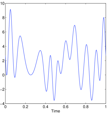
Figure 1: Left: Original signal; Right: Error of the IMF and the phase function.

The numerical results are shown in Fig. 1 and Fig. 2. In Fig. 1, we can see that our algorithm indeed recovers the exact decomposition of this signal. This is also consistent with the theoretical result we obtained in Theorem 2.1. The result shown in Fig. 1 is obtained by applying the non-uniform Fourier transform directly. As we proposed in our algorithm, for a well-resolved signal, it is more efficient to use a combination of interpolation and FFT. This procedure would introduce some interpolation error, however the computation is accelerated tremendously.

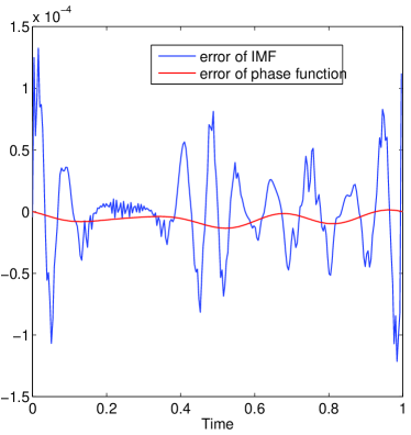
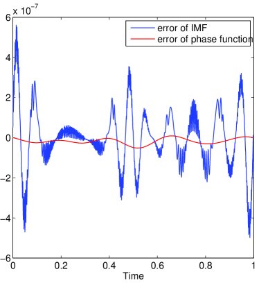
Figure 2: Left: Error of the IMF and the phase function with 256 uniform samples; Right: Error of the IMF and the phase function with 1024 uniform samples.

As we see in Fig. 2, if we use the FFT-based algorithm, the error increase to the order of $10^{-4}$ instead of $10^{-11}$ in the previous result when we used the non-uniform Fourier transform. If we increase the number of sample points to 1024, the order of error decreases to $10^{-7}$. This indicates that the main source of error comes from the interpolation error.

In our previous paper [12], we have shown many numerical results to demonstrate the stability of our algorithm. These numerical examples confirm the theoretical results presented in Theorem 2.2 and Theorem 2.3. We will not reproduce these numerical examples in this paper.

Example 2: Exact recovery for a signal with random samples

The second example is designed to confirm the result of Theorem 3.1. This example shows that for a signal with a sparse structure, our algorithm is capable of producing the exact decomposition even if it is poorly sampled. The signal is given below in (4).

$$\theta=200\pi t-10\cos 2\pi t-2\sin 4\pi t,\quad\overline{\theta}=\theta/(100)$$

$$a_{0}=\cos\overline{\theta},\quad a_{1}=3+\cos\overline{\theta}+\sin 2\overline{\theta}$$

$$f=a_{0}+a_{1}\cos\theta.$$ (134)

The number of sample points is set to be 120. These sample points are selected at random over 4096 uniformly distributed points. On average, there are only 1.2 points in each period of the signal. We test 100 independent samples and our algorithm is able to recover the signal for 97 samples, which gives $97\%$ success rate. Fig. 3 gives one of the successful samples.

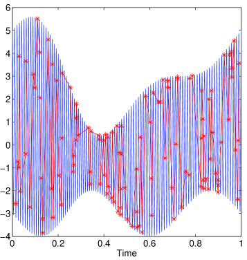
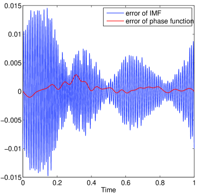
Figure 3: Left: Original signal and the sample points; Right: Error of the IMF and phase function.

The right panel of Fig. 3 shows that the order of error is $10^{-2}$ for IMF and $10^{-3}$ for the phase function. In the computation, the $l^{1}$ optimization problem is solved approximately in each step of the iteration. This is the reason that the error is much larger than the round-off error of the computer. If we increase the accuracy in solving the $l^{1}$ optimization problem, the algorithm would give a more accurate result. However the computational cost also increases as a consequence. We also reduce the number of sample points to 80 and carry out the same test for 100 times. In this case, the recovery rate was 46 out of 100.

Example 3: Approximate recovery for a signal with random samples

In this example, we will check the stability of our algorithm for a sparsely sampled signal. The signal is generated by (4),

$$\theta=\theta_{0}+0.1\sin(120\pi t),$$

$$a_{0}=\cos(2\pi t),\quad a_{1}=3+\cos(2\pi t)+\sin(4\pi t)$$

$$f=a_{0}+a_{1}\cos\theta+0.1X(t).$$ (135)

where $\theta_{0}$ is the $\theta$ given in (4), and $X(t)$ is the Gaussian noise with standard deviation $\sigma^{2}=1$. Based on the signal in the previous example, we add one small high frequency component on the phase function such that this high frequency part cannot be captured during the iteration. Moreover, $a_{0}$ and $a_{1}$ are not exactly sparse over the Fourier basis in the $\theta$-space. We also add a white noise to the original signal to make it even more challenging to decompose.

In this example, when the number of sample points is 120, our method can give 92 successful recoveries in 100 independent tests. Fig. 4 gives one of the successful recoveries obtained by our algorithm. Due to the truncation error and the noise, the error becomes much larger than that in the previous example. But all the errors are comparable with the magnitude of the truncation error and noise, which shows that our method has good stability even for signals with rare samples. When the number of samples is reduced to 80, the recovery rate drops to 40 out of 100.

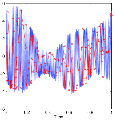
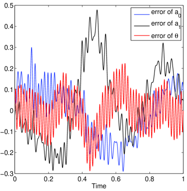
Figure 4: Left:Original signal (blue) and the sample points (red) in Ex 3; Right: Errors of $a_{0}$, $a_{1}$ and $\theta$.

5 Concluding remarks

In this paper, we analysed the convergence of the data-driven time-frequency analysis method proposed in [12]. First, we considered the case when the number of sample points is large enough. We proved that the algorithm we developed would converge to the exact decomposition if the signal has an intrinsic sparsity structure in the coordinate determined by the phase function. We also proved the convergence of our method with an approximate decomposition when the signal does not have an exact sparse structure but its spectral coefficients have a fast decay.

We also considered the more challenging case when only a few number of samples are given which do not resolve the original signal accurately. In this case, we need to solve a $l^{1}$ minimization problem which is computationally more expensive. We proved the stability and convergence of our method by using some results developed in compressive sensing. As in compressive sensing, the convergence and stability of our method assumes that certain $S$-restricted isometry condition is satisfied. We proved that for each fixed step in the iteration, this $S$-restricted isometry condition is satisfied with an overwhelming probability if the sample points are selected at random.

We presented numerical evidence to support our theoretical results. Our numerical results confirmed the theoretical results in all cases that we considered.

We are currently working on the convergence of the data-driven time-frequency analysis method for non-periodic signals. Our extensive numerical results seem to indicate that our method also converges for non-periodic signals. The theoretical analysis for this problem is more challenging. We will report the result in a subsequent paper.

Acknowledgments. This work was in part supported by the AFOSR MURI grant FA9550-09-1-0613, a DOE grant DE-FG02-06ER25727, and a NSF grant DMS-0908546. The research of Dr. Z. Shi was in part supported by a NSFC Grant 11201257.

Appendix A: Error of the envelope functions

Suppose

$$f(t)=f_{0}(t)+f_{1}(t)\cos\theta$$ (136)

is the signal we want to decompose.

Let $a^{m}=f_{1}\cos\Delta\theta^{m},\quad b^{m}=f_{1}\sin\Delta\theta^{m}$, then, we have

$$f=f_{0}+a^{m}\cos\theta^{m}-b^{m}\sin\theta^{m}.$$ (137)

Let $L^{m}=\frac{\theta^{m}(T)-\theta^{m}(0)}{2\pi}$ and $\overline{\theta}^{m}=\theta^{m}/(2\pi L^{m})$. Then, we have

$$f=f_{0}+a^{m}\cos 2\pi L^{m}\overline{\theta}^{m}-b^{m}\sin 2\pi L^{m}\overline{\theta}^{m}.$$ (138)

Define the Fourier transform in $\overline{\theta}$-space as:

$$\widehat{f}_{\theta^{m}}=\int_{0}^{1}f(t)e^{-i2\pi k\overline{\theta}^{m}}d\overline{\theta}^{m}.$$ (139)

Applying Fourier transform to both sides of (138), we have

$$\widehat{f}_{\theta^{m}}(k)=\widehat{f}_{0,\theta^{m}}(k)+\frac{1}{2}\left(\widehat{a}^{m}_{\theta^{m}}(k+L^{m})+\widehat{a}^{m}_{\theta^{m}}(k-L)\right)-\frac{i}{2}\left(\widehat{b}^{m}_{\theta^{m}}(k+L^{m})-\widehat{b}^{m}_{\theta^{m}}(k-L^{m})\right).\quad\quad$$ (140)

Then, we get

$$\widehat{a}^{m}_{\theta^{m}}(k)-i\widehat{b}^{m}_{\theta^{m}}(k) = 2\widehat{f}_{\theta^{m}}(k-L^{m})-2\widehat{f}_{0,\theta^{m}}(k-L^{m})-\widehat{a}^{m}_{\theta^{m}}(k-2L^{m})-i\widehat{b}^{m}_{\theta^{m}}(k-2L^{m}),$$

$$\widehat{a}^{m}_{\theta^{m}}(k)+i\widehat{b}^{m}_{\theta^{m}}(k) = 2\widehat{f}_{\theta^{m}}(k+L^{m})-2\widehat{f}_{0,\theta^{m}}(k+L^{m})-\widehat{a}^{m}_{\theta^{m}}(k+2L^{m})+i\widehat{b}^{m}_{\theta^{m}}(k+2L^{m}).$$

It is easy to solve for $\widehat{a}^{m}_{\theta^{m}}$ and $\widehat{b}^{m}_{\theta^{m}}$ to obtain:

$$\widehat{a}^{m}_{\theta^{m}}(k) = \widehat{f}_{\theta^{m}}(k+L^{m})+\widehat{f}_{\theta^{m}}(k-L^{m})-\left[\widehat{f}_{0,\theta^{m}}(k+L^{m})+\widehat{f}_{0,\theta^{m}}(k-L^{m})\right.$$ (141)

$$\left.+\frac{1}{2}\left(\widehat{a}^{m}_{\theta^{m}}(k+2L^{m})+\widehat{a}^{m}_{\theta^{m}}(k-2L^{m})\right)-\frac{i}{2}\left(\widehat{b}^{m}_{\theta^{m}}(k+2L^{m})-\widehat{b}^{m}_{\theta^{m}}(k-2L^{m})\right)\right],\quad\quad$$

$$\widehat{b}^{m}_{\theta^{m}}(k) = -i\left(\widehat{f}_{\theta^{m}}(k+L^{m})-\widehat{f}_{\theta^{m}}(k-L^{m})\right)+i\left[\widehat{f}_{0,\theta^{m}}(k+L^{m})-\widehat{f}_{0,\theta^{m}}(k-L^{m})\right.$$ (142)

$$\left.+\frac{1}{2}\left(\widehat{a}^{m}_{\theta^{m}}(k+2L^{m})-\widehat{a}^{m}_{\theta^{m}}(k-2L^{m})\right)-\frac{i}{2}\left(\widehat{b}^{m}_{\theta^{m}}(k+2L^{m})+\widehat{b}^{m}_{\theta^{m}}(k-2L^{m})\right)\right].$$

In our algorithm, $\mathcal{F}_{\theta^{m}}(\widetilde{a}^{m})$ and $\mathcal{F}_{\theta^{m}}(\widetilde{b}^{m})$ are approximated in the following way:

$$\widehat{\widetilde{a}}^{m}_{\theta^{m}}(k) = \left\{\begin{array}[]{cc}\widehat{f}_{\theta^{m}}(k+L^{m})+\widehat{f}_{\theta^{m}}(k-L^{m}),&-L^{m}/2\leq k\leq L^{m}/2,\\ 0,&otherwise.\end{array}\right.$$ (145)

$$\widehat{\widetilde{b}}^{m}_{\theta^{m}}(k) = \left\{\begin{array}[]{cc}-i(\widehat{f}_{\theta^{m}}(k+L^{m})-\widehat{f}_{\theta^{m}}(k-L^{m})),&-L^{m}/2\leq k\leq L^{m}/2,\\ 0,&otherwise.\end{array}\right.$$ (148)

Then, we can get the error of the approximation in the spectral space:

$$\widehat{\Delta a}^{m}_{\theta^{m}}(k)=\left\{\begin{array}[]{cl}-\left[\widehat{f}_{0,\theta^{m}}(k+L^{m})+\widehat{f}_{0,\theta^{m}}(k-L^{m})+\frac{1}{2}\left(\widehat{a}^{m}_{\theta^{m}}(k+2L^{m})+\widehat{a}^{m}_{\theta^{m}}(k-2L^{m})\right)\right.\\ \hskip 28.45274pt\left.-\frac{i}{2}\left(\widehat{b}^{m}_{\theta^{m}}(k+2L^{m})-\widehat{b}^{m}_{\theta^{m}}(k-2L^{m})\right)\right],&|k|\leq L^{m}/2,\\ \widehat{a}^{m}_{\theta^{m}}(k),&|k|>L^{m}/2.\end{array}\right.$$

$$\widehat{\Delta b}^{m}_{\theta^{m}}(k)=\left\{\begin{array}[]{cl}i\left[\widehat{f}_{0,\theta^{m}}(k+L^{m})-\widehat{f}_{0,\theta^{m}}(k-L^{m})+\frac{1}{2}\left(\widehat{a}^{m}_{\theta^{m}}(k+2L^{m})-\widehat{a}^{m}_{\theta^{m}}(k-2L^{m})\right)\right.\\ \left.-\frac{i}{2}\left(\widehat{b}^{m}_{\theta^{m}}(k+2L^{m})+\widehat{b}^{m}_{\theta^{m}}(k-2L^{m})\right)\right],&|k|\leq L^{m}/2,\\ \widehat{b}^{m}_{\theta^{m}}(k),&|k|>L^{m}/2.\end{array}\right.$$

Thus, we have the following inequality for the $l^{1}$ norm of the error in the spectral space:

$$|\Delta a^{m}| \leq \|\widehat{\Delta a}^{m}_{\theta^{m}}\|_{1}$$ (151)

$$\leq 2\sum_{\frac{L^{m}}{2}<k<\frac{3}{2}L^{m}}\left|\widehat{f}_{0,\theta^{m}}(k)\right|+\sum_{\frac{3}{2}L^{m}<k<\frac{5}{2}L^{m}}\left(\left|\widehat{a}^{m}_{\theta^{m}}(k)\right|+\left|\widehat{b}^{m}_{\theta^{m}}(k)\right|\right)+\sum_{|k|>\frac{L^{m}}{2}}\left|\widehat{a}^{m}_{\theta^{m}}(k)\right|.\quad\quad\quad$$

Similarly, we get

$$|\Delta b^{m}|\leq 2\sum_{\frac{L^{m}}{2}<k<\frac{3}{2}L^{m}}\left|\widehat{f}_{0,\theta^{m}}(k)\right|+\sum_{\frac{3}{2}L^{m}<k<\frac{5}{2}L^{m}}\left(\left|\widehat{a}^{m}_{\theta^{m}}(k)\right|+\left|\widehat{b}^{m}_{\theta^{m}}(k)\right|\right)+\sum_{|k|>\frac{L^{m}}{2}}\left|\widehat{b}^{m}_{\theta^{m}}(k)\right|.\quad\quad\quad$$ (152)

In the above derivation, we assume that the Fourier transform of $f$ in $\theta^{m}$-space can be calculated exactly. If only approximate Fourier transform is available, denoted as $\widehat{\widetilde{f}}_{\theta^{m}}$, such as the signal with sparse samples we discussed in Section 3, there would be an extra term in the estimates of $\Delta a^{m}$ and $\Delta b^{m}$,

$$|\Delta a^{m}| \leq 2\sum_{\frac{L^{m}}{2}<k<\frac{3}{2}L^{m}}\left|\widehat{f}_{0,\theta^{m}}(k)\right|+\sum_{\frac{3}{2}L^{m}<k<\frac{5}{2}L^{m}}\left(\left|\widehat{a}^{m}_{\theta^{m}}(k)\right|+\left|\widehat{b}^{m}_{\theta^{m}}(k)\right|\right)$$ (153)

$$+\sum_{|k|>\frac{L^{m}}{2}}\left|\widehat{a}^{m}_{\theta^{m}}(k)\right|+2\sum_{\frac{L^{m}}{2}<k<\frac{3}{2}L^{m}}\left|\widehat{f}_{\theta^{m}}(k)-\widehat{\widetilde{f}}_{\theta^{m}}(k)\right|,$$

$$|\Delta b^{m}| \leq 2\sum_{\frac{L^{m}}{2}<k<\frac{3}{2}L^{m}}\left|\widehat{f}_{0,\theta^{m}}(k)\right|+\sum_{\frac{3}{2}L^{m}<k<\frac{5}{2}L^{m}}\left(\left|\widehat{a}^{m}_{\theta^{m}}(k)\right|+\left|\widehat{b}^{m}_{\theta^{m}}(k)\right|\right)$$ (154)

$$+\sum_{|k|>\frac{L^{m}}{2}}\left|\widehat{b}^{m}_{\theta^{m}}(k)\right|+2\sum_{\frac{L^{m}}{2}<k<\frac{3}{2}L^{m}}\left|\widehat{f}_{\theta^{m}}(k)-\widehat{\widetilde{f}}_{\theta^{m}}(k)\right|.$$

Appendix B: Estimates of $\widehat{f}_{0,\theta^{m}}(\omega)$, $\widehat{a}^{m}_{\theta^{m}}(\omega)$ and $\widehat{b}^{m}_{\theta^{m}}(\omega)$in Theorem 2.1.

We first estimate $f_{0}$. We have

$$|\widehat{f}_{0,\theta^{m}}(\omega)| = \left|\int_{0}^{1}f_{0}(t)e^{-i2\pi\omega\overline{\theta}^{m}}d\overline{\theta}^{m}\right|$$ (155)

$$= \int_{0}^{1}\sum_{|k|\leq M_{1}}\widehat{f}_{0,\theta}(k)e^{i2\pi(k\overline{\theta}-\omega\overline{\theta}^{m})}d\overline{\theta}^{m}$$

$$= \sum_{|k|\leq M_{1}}\widehat{f}_{0,\theta}(k)\int_{0}^{1}e^{i2\pi(k\overline{\theta}-\omega\overline{\theta}^{m})}d\overline{\theta}^{m}$$

$$= \left|\sum_{|k|\leq M_{1}}\widehat{f}_{0,\theta}(k)\int_{0}^{1}e^{i2\pi(\alpha k-\omega)\overline{\theta}^{m}}e^{ik\Delta\theta^{m}/L}d\overline{\theta}^{m}\right|,$$

where $\alpha=L^{m}/L$. In the last equality, we have used the fact that $\theta=2\pi L\overline{\theta},\;\theta^{m}=2\pi L^{m}\overline{\theta}^{m}$ and $\theta=\theta^{m}+\Delta\theta^{m}$.

Using Lemma 2.1, we obtain for any $|\omega|>L/2$ that

$$|\widehat{f}_{0,\theta^{m}}(\omega)| \leq \left|\sum_{|k|\leq M_{1}}\widehat{f}_{0,\theta}(k)\int_{0}^{1}e^{i2\pi(\alpha k-\omega)\overline{\theta}^{m}}e^{ik\Delta\theta^{m}/L}d\overline{\theta}^{m}\right|$$ (156)

$$\leq C_{0}\sum_{|k|\leq M_{1}}\frac{QM_{0}^{n}}{|\omega-\alpha k|^{n}}\sum_{j=1}^{n}\left|\frac{k}{L}\right|^{j}(2\pi M_{0})^{-j}\|\mathcal{F}_{\theta^{m}}[(\Delta\theta^{m})^{\prime}]\|_{1}^{j}$$

$$\leq 2C_{0}Q\left(\frac{|\omega|}{2}\right)^{-n}M_{0}^{n}M_{1}\sum_{j=1}^{n}\left(M_{1}\gamma/L\right)^{j},$$

where

$$Q=\frac{P\left(z,n\right)}{\left(\min(\overline{\theta}^{m})^{\prime}\right)^{n}},\quad z=\frac{\|\mathcal{F}[(\overline{\theta}^{m})^{\prime}]\|_{1}}{\min(\overline{\theta}^{m})^{\prime}},\quad\gamma=\frac{\|\mathcal{F}[(\Delta\theta^{m})^{\prime}]\|_{1}}{2\pi M_{0}}.$$ (157)

In the above derivation, we need to assume that $L\geq 4M_{1}$ such that $|\omega-\alpha k|\geq|\omega|/2$ for all $|\omega|\geq L/2$ and $|k|\leq M_{1}$.

If we further assume that $\gamma\leq 1/4$, we have

$$|\widehat{f}_{0,\theta^{m}}(\omega)| \leq C_{0}Q\left(\frac{|\omega|}{2}\right)^{-n}M_{0}^{n}M_{1}\gamma.$$ (158)

Next, we estimate $\widehat{a}^{m}_{\theta^{m}}$. The method of analysis is similar to the previous one, however the derivation is a little more complicated. We proceed as follows:

$$|\widehat{a}^{m}_{\theta^{m}}(\omega)| = \left|\int_{0}^{1}f_{1}(t)\cos\Delta\theta^{m}(t)e^{-i2\pi\omega\overline{\theta}^{m}}d\overline{\theta}^{m}\right|$$ (159)

$$\leq \frac{1}{2}\left|\int_{0}^{1}\sum_{|k|\leq M_{1}}f_{1,\theta}(k)e^{i2\pi k\overline{\theta}}(e^{i\Delta\theta}+e^{-i\Delta\theta})e^{-i2\pi\omega\overline{\theta}^{m}}d\overline{\theta}^{m}\right|$$

$$\leq \frac{1}{2}\left|\sum_{|k|\leq M_{1}}f_{1,\theta}(k)\int_{0}^{1}e^{i2\pi(\alpha k-\omega)\overline{\theta}^{m}}e^{i(k+L)\Delta\theta/L}d\overline{\theta}^{m}\right|$$

$$+\frac{1}{2}\left|\sum_{|k|\leq M_{1}}f_{1,\theta}(k)\int_{0}^{1}e^{i2\pi(\alpha k-\omega)\overline{\theta}^{m}}e^{i(k-L)\Delta\theta/L}d\overline{\theta}^{m}\right|.$$

For the first term in the above inequality, we have that for any $|\omega|>L/2$,

$$\left|\sum_{|k|\leq M_{1}}f_{1,\theta}(k)\int_{0}^{1}e^{i2\pi(\alpha k-\omega)\overline{\theta}^{m}}e^{i(k+L)\Delta\theta/L}d\overline{\theta}^{m}\right|$$ (160)

$$\leq C_{0}Q\sum_{|k|\leq M_{1}}\frac{M_{0}^{n}}{|\omega-\alpha k|^{n}}\sum_{j=1}^{n}\left|1+\frac{k}{L}\right|^{j}\gamma^{j}$$

$$\leq C_{0}Q\left(\frac{|\omega|}{2}\right)^{-n}M_{0}^{n}\sum_{j=1}^{n}2^{j-1}\gamma^{j}\sum_{|k|\leq M_{1}}\left(1+\left|\frac{k}{L}\right|^{j}\right)$$

$$\leq 4C_{0}Q\left(\frac{|\omega|}{2}\right)^{-n}M_{0}^{n}(2M_{1}+1)\gamma.$$

Here we also assume that $L\geq 4M_{1},\;\gamma\leq 1/4$. The definition of $Q$ and $\gamma$ can be found in (48).

For the second term in (159), we can get the same bound for $|\omega|\geq L/2$,

$$\left|\sum_{|k|\leq M_{1}}f_{1,\theta}(k)\int_{0}^{1}e^{i2\pi(\alpha k-\omega)\overline{\theta}^{m}}e^{i(k-L)\Delta\theta/L}d\overline{\theta}^{m}\right|\leq 4C_{0}Q\left(\frac{|\omega|}{2}\right)^{-n}M_{0}^{n}(2M_{1}+1)\gamma.$$ (161)

By combining (159),(160) and (161), we obtain a complete control of $\widehat{\overline{a}}$,

$$|\widehat{a}^{m}_{\theta^{m}}(\omega)| \leq 4C_{0}Q\left(\frac{|\omega|}{2}\right)^{-n}M_{0}^{n}(2M_{1}+1)\gamma,\quad\forall|\omega|\geq L/2.$$ (162)

Similarly, we can estimate $\widehat{b}^{m}_{\theta^{m}}$ by the same upper bound,

$$|\widehat{b}^{m}_{\theta^{m}}(\omega)| \leq 4C_{0}Q\left(\frac{|\omega|}{2}\right)^{-n}M_{0}^{n}(2M_{1}+1)\gamma,\quad\forall|\omega|\geq L/2.$$ (163)

Appendix C: Proof of Lemma 3.1

Proof.

Since $e^{i2\pi k\phi}$ is a periodic function over $[0,1]$, it can be represented by Fourier series:

$$e^{i2\pi k\phi(t)}=\sum_{l=-\infty}^{+\infty}d_{l}e^{i2\pi lt},\quad t\in[0,1],$$ (164)

where $d_{l}=\int_{0}^{1}e^{i2\pi k\phi(t)}e^{-i2\pi lt}dt$. By assumption, we have $\phi^{\prime}(t)\in V_{M_{0}}$. Thus, we get

$$\phi^{\prime}(t)=\sum_{j=-M_{0}}^{M_{0}}c_{j}e^{i2\pi jt},\quad t\in[0,1],$$ (165)

where $c_{j}=\int_{0}^{1}\overline{\theta}^{\prime}(t)e^{-i2\pi jt}dt$.

Then, we have

$$\frac{1}{L}\sum_{m=0}^{L-1}\phi^{\prime}(t_{m})e^{i2\pi k\phi(t_{m})}$$ (166)

$$= \frac{1}{L}\sum_{m=0}^{L-1}\sum_{j=-M_{0}}^{M_{0}}\sum_{l=-\infty}^{+\infty}c_{j}d_{l}e^{i2\pi(l+j)t_{m}}$$

$$= \frac{1}{L}\sum_{j=-M_{0}}^{M_{0}}\sum_{l=-\infty}^{+\infty}c_{j}d_{l}\sum_{m=0}^{L-1}e^{i2\pi(l+j)m/L}$$

$$= \sum_{j=-M_{0}}^{M_{0}}\sum_{p\in\mathbb{Z}}c_{j}d_{pL-j}$$

$$= \sum_{j=-M_{0}}^{M_{0}}c_{j}d_{-j}+\sum_{j=-M_{0}}^{M_{0}}\sum_{p\in\mathbb{Z},p\neq 0}c_{j}d_{pL-j}$$

$$= \int_{0}^{1}\overline{\theta}^{\prime}(t)e^{i2\pi k\phi(t)}dt+\sum_{j=-M_{0}}^{M_{0}}\sum_{p\in\mathbb{Z},p\neq 0}c_{j}d_{pL-j}$$

$$= \sum_{j=-M_{0}}^{M_{0}}\sum_{p\in\mathbb{Z},p\neq 0}c_{j}d_{pL-j}.$$

Using integration by parts, we have

$$|d_{l}| = |\int_{0}^{1}e^{i2\pi k\phi}e^{-i2\pi lt}dt|$$ (167)

$$= \frac{1}{|l|^{n}}\left|\int_{0}^{1}\left(\frac{d^{n}}{dt^{n}}e^{i2\pi k\phi}\right)e^{-i2\pi lt}dt\right|$$

$$\leq \frac{1}{|l|^{n}}\int_{0}^{1}\left|\left(\frac{d^{n}}{dt^{n}}e^{i2\pi k\phi}\right)\right|dt$$

$$\leq \frac{1}{|l|^{n}}\max_{t}\left|\left(\frac{d^{n}}{dt^{n}}e^{i2\pi k\phi}\right)\right|.$$

Using the inequality (32) in the proof of Lemma 2.1, and by a direct calculation, we can show that for any $n>0$, there exists $C(n)>0$, such that

$$\max_{t}\left|\left(\frac{d^{n}}{dt^{n}}e^{i2\pi k\phi}\right)\right| \leq C(n)\sum_{j=1}^{n}|k|^{j}M_{0}^{n-j}\|\widehat{\phi^{\prime}}\|_{1}^{j}=C(n)|k|M_{0}^{n-1}\|\widehat{\phi^{\prime}}\|_{1}\frac{\frac{|k|^{n}}{M_{0}^{n}}\|\widehat{\phi^{\prime}}\|_{1}^{n}-1}{\frac{|k|}{M_{0}}\|\widehat{\phi^{\prime}}\|_{1}-1}$$ (170)

$$\leq \left\{\begin{array}[]{cc}2C(n)|k|^{n}\|\widehat{\phi^{\prime}}\|_{1}^{n},&\frac{|k|}{M_{0}}\|\widehat{\phi^{\prime}}\|_{1}>2,\\ 2C(n)(2M_{0})^{n},&\frac{|k|}{M_{0}}\|\widehat{\phi^{\prime}}\|_{1}\leq 2.\end{array}\right.$$

As a result, we obtain

$$|d_{l}|\leq\left\{\begin{array}[]{cc}2C(n)\left|\frac{k\|\widehat{\phi^{\prime}}\|_{1}}{l}\right|^{n},&|k|\|\widehat{\phi^{\prime}}\|_{1}>2M_{0},\\ 2C(n)\left|\frac{2M_{0}}{l}\right|^{n},&|k|\|\widehat{\phi^{\prime}}\|_{1}\leq 2M_{0},\end{array}\right.$$ (173)

Finally, we derive the following estimate

$$\left|\sum_{j=-M_{0}}^{M_{0}}\sum_{p\in\mathbb{Z},p\neq 0}c_{j}d_{pL-j}\right|$$ (174)

$$\leq \sum_{p\in\mathbb{Z},p\neq 0}\sum_{j=-M_{0}}^{M_{0}}|c_{j}||d_{pL-j}|$$

$$\leq 2\sum_{j=-M_{0}}^{M_{0}}|c_{j}|\sum_{p=1}^{+\infty}\max_{j}|d_{pL-j}|$$

$$\leq 4C(n)\|\widehat{\phi^{\prime}}\|_{1}\sum_{p=1}^{+\infty}\max\left(\left|\frac{k\|\widehat{\phi^{\prime}}\|_{1}}{pL-M_{0}}\right|^{n},\left|\frac{2M_{0}}{pL-M_{0}}\right|^{n}\right)$$

$$\leq 4C(n)\|\widehat{\phi^{\prime}}\|_{1}\max\left(\left|\frac{k\|\widehat{\phi^{\prime}}\|_{1}}{L}\right|^{n},\left|\frac{2M_{0}}{L}\right|^{n}\right)\sum_{p=1}^{+\infty}(p-M_{0}/L)^{-n}$$

$$\leq 4\left(1-M_{0}/L\right)^{-n+1}\frac{C(n)}{n-1}\|\widehat{\phi^{\prime}}\|_{1}\max\left(\left|\frac{k\|\widehat{\phi^{\prime}}\|_{1}}{L}\right|^{n},\left|\frac{2M_{0}}{L}\right|^{n}\right).$$

∎

References

• [1] B. Boashash, Time-Frequency Signal Analysis: Methods and Applications, Longman-Cheshire, Melbourne and John Wiley Halsted Press, New York, 1992.
• [2] A. M. Bruckstein, D. L. Donoho, M. Elad, From sparse solutions of systems of equations to sparse modeling of signals and images, SIAM Review, 51, pp. 34-81, 2009.
• [3] E. Cand$\grave{\mbox{e}}$s and T. Tao, Decoding by linear programming, IEEE Trans. on Information Theory, 52(12), pp. 5406-5425, 2006.
• [4] E. Cand$\grave{\mbox{e}}$s and T. Tao, Near optimal signal recovery from random projections: Universal encoding strategies?, IEEE Trans. on Information Theory, 52(12), pp. 5406-5425, 2006.
• [5] E. Cand$\grave{\mbox{e}}$s and T. Tao, Near optimal signal recovery from random projections: Universal encoding strategies?, IEEE Trans. on Information Theory, 52(12), pp. 5406-5425, 2006.
• [6] E. Candes, J. Romberg, and T. Tao, Robust uncertainty principles: Exact signal recovery from highly incomplete frequency information, IEEE Trans. Inform. Theory, 52, pp. 489-509, 2006.
• [7] E. Candes, J. Romberg, and T. Tao, Stable signal recovery from incomplete and inaccurate measurements, Comm. Pure and Appl. Math., 59, pp. 1207-1223, 2006.
• [8] I. Daubechies, Ten Lectures on Wavelets, CBMS-NSF Regional Conference Series on Applied Mathematics, Vol. 61, SIAM Publications, 1992.
• [9] D. L. Donoho, Compressed sensing, IEEE Trans. Inform. Theory, 52, pp. 1289-1306, 2006.
• [10] P. Flandrin, Time-Frequency/Time-Scale Analysis, Academic Press, San Diego, CA, 1999.
• [11] D. Gabor, Theory of communication, J. IEE., 93, pp. 426-457, 1946.
• [12] T. Y. Hou and Z. Shi, Data-Drive Time-Frequency analysis, Applied and Comput. Harmonic Analysis, accepted, 2012.
• [13] N. E. Huang et al., The empirical mode decomposition and the Hilbert spectrum for nonlinear and non-stationary time series analysis, Proc. R. Soc. Lond. A, 454 (1998), pp. 903-995.
• [14] D. L. Jomes and T. W. Parks, A high resolution data-adaptive time-frequency representation, IEEE Trans. Acoust. Speech Signal Process, 38, pp. 2127-2135, 1990.
• [15] P. J. Loughlin and B. Tracer, On the amplitude - and frequency-modulation decomposition of signals, J. Acoust. Soc. Am., 100, pp. 1594-1601, 1996.
• [16] B. C. Lovell, R. C. Williamson and B. Boashash, The relationship between instantaneous frequency and time-frequency representations, IEEE Trans. Signal Process, 41, pp. 1458-1461, 1993.
• [17] S. Mallat and Z. Zhang, Matching pursuit with time-frequency dictionaries, IEEE Trans. Signal Process, 41, pp. 3397-3415, 1993.
• [18] S. Mallat, A wavelet tour of signal processing: the Sparse way, Academic Press, 2009.
• [19] W. K. Meville, Wave modulation and breakdown, J. Fluid Mech., 128, pp. 489-506, 1983.
• [20] S. Olhede and A. T. Walden, The Hilbert spectrum via wavelet projections, Proc. Roy. Soc. London A, 460, pp. 955-975, 2004.
• [21] B. Picinbono, On instantaneous amplitude and phase signals, IEEE Trans. Signal Process, 45 (1997), pp. 552-560.
• [22] S. Qian and D. Chen, Joint Time-Frequency Analysis: Methods and Applications, Prentice Hall, 1996.
• [23] S. O. Rice, Mathematical analysis of random noise, Bell Syst. Tech. J., 23, pp. 282-310, 1944.
• [24] J. Shekel, Instantaneous frequency, Proc. IRE, 41 , pp. 548-548, 1953.
• [25] J. Tropp and A. Gilbert, Signal recovery from random measurements via Orthogonal Matching Pursuit, IEEE Trans. Inform. Theory, 53, pp. 4655-4666, 2007.
• [26] B. Van der Pol, The fundamental principles of frequency modulation, Proc. IEE, 93, pp. 153-158, 1946.
• [27] Z. Wu and N. E. Huang, Ensemble Empirical Mode Decomposition: a noise-assisted data analysis method, Advances in Adaptive Data Analysis, 1, pp. 1-41, 2009.