Upper bound on the total number of knot $n$-mosaics

Abstract.

Lomonaco and Kauffman introduced a knot mosaic system to give a definition of a quantum knot system which can be viewed as a blueprint for the construction of an actual physical quantum system. A knot $n$-mosaic is an $n\times n$ matrix of 11 kinds of specific mosaic tiles representing a knot or a link by adjoining properly that is called suitably connected. $D_{n}$ denotes the total number of all knot $n$-mosaics. Already known is that $D_{1}=1$, $D_{2}=2$, and $D_{3}=22$. In this paper we establish the lower and upper bounds on $D_{n}$

$$\frac{2}{275}(9\cdot 6^{n-2}+1)^{2}\cdot 2^{(n-3)^{2}}\ \leq\ D_{n}\ \leq\ \frac{2}{275}(9\cdot 6^{n-2}+1)^{2}\cdot(4.4)^{(n-3)^{2}}.$$

and find the exact number of $D_{4}=2594$.

1. Introduction

Knot theory and other areas of topology have made propound impact on quantum field theory, quantum computation and complexity of computation. Lomonaco and Kauffman introduced a knot mosaic system to set the foundation for a quantum knot system in the series of papers [2, 5, 6, 7, 8, 9]. This paper was inspired from an open question about the enumeration of knot mosaics in [7].

Throughout this paper we will frequently use the term “knot” to mean either a knot or a link for simplicity of exposition. Let $\mathbb{T}$ denote the set of the following $11$ symbols which are called mosaic tiles;

For a positive integer $n$, we define an $n$-mosaic as an $n\times n$ matrix $M=(M_{ij})$ of mosaic tiles. We denote the set of all $n$-mosaics by $\mathbb{M}^{(n)}$. Obviously $\mathbb{M}^{(n)}$ has $11^{n^{2}}$ elements. A connection point of a tile is defined as the midpoint of a mosaic tile edge which is also the endpoint of a curve drawn on the tile. Then each tile has zero, two or four connection points as follows;

We say that two tiles in a mosaic are contiguous if they lie immediately next to each other in either the same row or the same column. A mosaic tile within a mosaic is said to be suitably connected if each of its connection points touches a connection point of a contiguous tile. A knot $n$-mosaic is an $n$-mosaic in which all tiles are suitably connected. Then a knot $n$-mosaic represents a specific knot. In Figure 1, we draw three examples of mosaics; a 4-mosaic, the Hopf link 4-mosaic and the trefoil knot 4-mosaic.

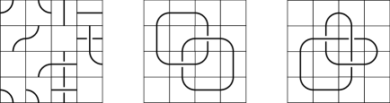
Figure 1. Three examples of 4-mosaics

As an analog to the planar isotopy moves and the Reidemeister moves for standard knot diagrams, Lomonaco and Kauffman created for knot mosaics the $11$ mosaic planar isotopy moves and the mosaic Reidemeister moves in [7]. They conjectured that for any two tame knots (or links) $K_{1}$ and $K_{2}$, and their arbitrary chosen mosaic representatives $M_{1}$ and $M_{2}$, respectively, $K_{1}$ and $K_{2}$ are of the same knot type if and only if $M_{1}$ and $M_{2}$ are of the same knot mosaic type. This means that tame knot theory and knot mosaic theory are equivalent. Kuriya and Shehab [3] proved that Lomonaco-Kauffman conjecture is true.

Lomonaco and Kauffman also proposed a dozen of open questions relevant to quantum knot mosaics. One natural question is how many knot $n$-mosaics are there. Let $\mathbb{K}^{(n)}$ denote the subset of $\mathbb{M}^{(n)}$ of all knot $n$-mosaics, and $D_{n}$ the total number of elements of $\mathbb{K}^{(n)}$. The main theme in this paper is to establish upper and lower bounds on $D_{n}$. Already known is that $D_{1}=1$, $D_{2}=2$ and $D_{3}=22$, for which the complete table of $\mathbb{K}^{(3)}$ is in Appendix A in [7]. One might gave a very loose upper bound $11^{n^{2}}$.

Theorem 1.

For an integer $n\geq 3$,

$$\frac{2}{275}(9\cdot 6^{n-2}+1)^{2}\cdot 2^{(n-3)^{2}}\ \leq\ D_{n}\ \leq\ \frac{2}{275}(9\cdot 6^{n-2}+1)^{2}\cdot(4.4)^{(n-3)^{2}}.$$

Theorem 2.

$D_{4}=2594$.

Recently, the authors announced several improved results on $D_{n}$ in the series of papers. They concerned the exact number of $D_{n}$ for small $n=4,5,6$ [1], the state matrix algorithm, so called, producing the exact enumeration of general $D_{n}$ that uses recursion formula of state matrices [11], and more precise bounds of the quadratic exponential growth ratio of $D_{n}$ [10].

Another interesting question relevant to knot mosaics is the mosaic number $m(K)$ of a knot $K$ as the smallest integer $n$ for which $K$ is representable as a knot $n$-mosaic. Is this mosaic number related to the crossing number of a knot? As an concrete answer, the authors [4] established an upper bound on the mosaic number as follows; if $K$ be a nontrivial knot or a non-split link except the Hopf link, then $m(K)\leq c(K)+1$, and moreover if $K$ is prime and non-alternating except $6^{3}_{3}$, then $m(K)\leq c(K)-1$. Note that the mosaic number of the Hopf link is 4, and the prime and non-alternating $6^{3}_{3}$ link is 6, even though their crossing numbers are 2 and 6, respectively.

2. Proof of Theorem 1

For $n\geq 3$, $\mathbb{K}^{(n)}$ is the set of knot $n$-mosaics, so each mosaic is filled by suitably connected $n^{2}$ mosaic tiles entirely. $\mathbb{K}^{(n)}_{1}$ denotes the set of so called $n$-quasimosaics each of which is filled by suitably connected $2n-3$ mosaic tiles only at $M_{1j}$ and $M_{i1}$, $i,j=1,2,\cdots,n-1$. It is indeed a part of a knot $n$-mosaic, and so possibly has connection points on the boundary contained in the interior of the knot $n$-mosaic. Similarly $\mathbb{K}^{(n)}_{2}$ denotes the set of $n$-quasimosaics each of which is filled by suitably connected $4n-8$ tiles at $M_{1j}$, $M_{2j}$, $M_{i1}$, and $M_{i2}$, $i,j=1,2,\cdots,n-1$. Also $\mathbb{K}^{(n)}_{3}$ denotes the set of $n$-quasimosaics each of which is filled by suitably connected $(n-1)^{2}$ tiles at $M_{ij}$, $i,j=1,2,\cdots,n-1$. Let $d_{1}$, $d_{2}$ and $d_{3}$ denote the numbers of elements of $\mathbb{K}^{(n)}_{1}$, $\mathbb{K}^{(n)}_{2}$ and $\mathbb{K}^{(n)}_{3}$, respectively. See three typical examples of elements of $\mathbb{K}^{(6)}_{1}$, $\mathbb{K}^{(6)}_{2}$ and $\mathbb{K}^{(6)}_{3}$ in Figure 2.

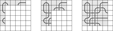
Figure 2. Three elements of $\mathbb{K}^{(6)}_{1}$, $\mathbb{K}^{(6)}_{2}$ and $\mathbb{K}^{(6)}_{3}$

For simplicity of exposition, a mosaic tile is called $t$-cp if it has a connection point on its top edge, and similarly $b$-, $l$- or $r$-cp when on its bottom, left or right edge, respectively. Sometimes we use two letters, for example, $tl$-cp in the case of both $t$-cp and $l$-cp. We use the sign $\hat{}$ for negation such as $\hat{t}$-cp means not $t$-cp, $\hat{t}\hat{l}$-cp means both $\hat{t}$-cp and $\hat{l}$-cp, and $\widehat{tl}$-cp (which is differ from $\hat{t}\hat{l}$-cp) means not $tl$-cp, i.e. $\hat{t}l$-, $t\hat{l}$- or $\hat{t}\hat{l}$-cp.

First we figure out $\mathbb{K}^{(n)}_{1}$ and determine the number $d_{1}$.

Lemma 3.

$d_{1}=2^{2n-3}$.

Proof.

We use the induction on $n$. The first mosaic tile $M_{11}$ has 2 choices whether $T_{0}$ or $T_{2}$. The next tile $M_{12}$ has always 2 choices after any choices of $M_{11}$ as follows; if $M_{11}=T_{0}$, then $M_{12}$ is $\hat{t}\hat{l}$-cp, so $M_{12}$ is either $T_{0}$ or $T_{2}$, or if $M_{11}=T_{2}$, then $M_{12}$ must be $\hat{t}l$-cp to be suitably connected, so $M_{12}$ is either $T_{1}$ or $T_{5}$. By the same reason each $M_{1j}$, $j=3,\cdots,n-1$, has always 2 choices; if $M_{1(j-1)}$ is $\hat{r}$-cp, then $\hat{t}\hat{l}$-cp $M_{1j}$ is either $T_{0}$ or $T_{2}$, or if $M_{1(j-1)}$ is $r$-cp, then $\hat{t}l$-cp $M_{1j}$ is either $T_{1}$ or $T_{5}$. We can follow the same argument when we choose mosaic tiles $M_{i1}$, $i=2,\cdots,n-1$. Thus if $M_{(i-1)1}$ is $\hat{b}$-cp, then $\hat{t}\hat{l}$-cp $M_{i1}$ is either $T_{0}$ or $T_{2}$, or if $M_{(i-1)1}$ is $b$-cp, then $t\hat{l}$-cp $M_{i1}$ is either $T_{3}$ or $T_{6}$. Therefore each tile has exactly 2 choices. Since each $n$-quasimosaic of $\mathbb{K}^{(n)}_{1}$ consists of $2n-3$ mosaic tiles,

$d_{1}=2^{2n-3}$. ∎

Fact 1. For any $j=2,\cdots,n-1$, exactly the half of $\mathbb{K}^{(n)}_{1}$ have $b$-cp $M_{1j}$’s and the rest half have $\hat{b}$-cp $M_{1j}$’s. Similarly for any $i=2,\cdots,n-1$, exactly the half of $\mathbb{K}^{(n)}_{1}$ have $r$-cp $M_{i1}$’s and the rest half have $\hat{r}$-cp $M_{i1}$’s.

Fact 2. For any $i,j=2,\cdots,n-1$, $M_{ij}$ is one of $T_{4}$, $T_{7}$, $T_{8}$, $T_{9}$ or $T_{10}$ if it is $tl$-cp, either $T_{1}$ or $T_{5}$ if $\hat{t}l$-cp, either $T_{3}$ or $T_{6}$ if $t\hat{l}$-cp, and either $T_{0}$ or $T_{2}$ if $\hat{t}\hat{l}$-cp. Therefore each $M_{ij}$ has 5 choices of mosaic tiles if it is $tl$-cp, and 2 choices if it is $\widehat{tl}$-cp.

Next we figure out $\mathbb{K}^{(n)}_{2}$ and determine the number $d_{2}$.

Lemma 4.

$d_{2}=\frac{2}{275}(9\cdot 6^{n-2}+1)^{2}$.

Proof.

Similar to the definitions of $\mathbb{K}^{(n)}_{2}$ and $d_{2}$, let $\mathbb{K}^{(n)}_{2j}$, $j=2,\cdots,n-1$, denote the set of all $n$-quasimosaics each of which is filled by suitably connected mosaic tiles as in $\mathbb{K}^{(n)}_{1}$ and more tiles at $M_{2k}$, $k=2,\cdots,j$. Let $d_{2j}$ denote the number of elements of $\mathbb{K}^{(n)}_{2j}$.

First we fill the mosaic tile $M_{22}$. By Fact 1, exactly $(\frac{1}{2})^{2}d_{1}$ elements of $\mathbb{K}^{(n)}_{1}$ have $tl$-cp $M_{22}$’s to be suitably connected, and the rest $\frac{3}{4}d_{1}$ elements have $\widehat{tl}$-cp $M_{22}$’s. By Fact 2, $d_{22}=\frac{1}{4}d_{1}\cdot 5+\frac{3}{4}d_{1}\cdot 2=\frac{11}{4}d_{1}$. Note that among all $d_{22}$ elements of $\mathbb{K}^{(n)}_{22}$, $\frac{1}{4}d_{1}\cdot 4+\frac{3}{4}d_{1}\cdot 1=\frac{7}{4}d_{1}=\frac{7}{11}d_{22}$ elements have $r$-cp $M_{22}$’s. Let $p_{2}=\frac{7}{11}$.

Now we use the induction again. For any $j=3,\cdots,n-1$, the same argument above guarantees that exactly $\frac{1}{2}p_{j-1}\cdot d_{2(j-1)}$ elements of $\mathbb{K}^{(n)}_{2(j-1)}$ can be suitably connected with $tl$-cp $M_{2j}$’s, and the rest elements with $\widehat{tl}$-cp $M_{2j}$’s. Thus $d_{2j}=\frac{1}{2}p_{j-1}\cdot d_{2(j-1)}\cdot 5+(1-\frac{1}{2}p_{j-1})\cdot d_{2(j-1)}\cdot 2=(2+\frac{3}{2}p_{j-1})\cdot d_{2(j-1)}$. Then among all $d_{2j}$ elements of $\mathbb{K}^{(n)}_{2j}$, $\frac{1}{2}p_{j-1}\cdot d_{2(j-1)}\cdot 4+(1-\frac{1}{2}p_{j-1})\cdot d_{2(j-1)}\cdot 1=(1+\frac{3}{2}p_{j-1})\cdot d_{2(j-1)}=\frac{2+3p_{j-1}}{4+3p_{j-1}}\cdot d_{2j}$ elements have $r$-cp $M_{2j}$’s. Let $p_{j}=\frac{2+3p_{j-1}}{4+3p_{j-1}}$.

Therefore $d_{2(n-1)}=d_{1}\cdot\frac{11}{4}\cdot(2+\frac{3}{2}p_{2})\cdots(2+\frac{3}{2}p_{n-2})$. Since $p_{j}=\frac{2\cdot 6^{j}-2}{3\cdot 6^{j}+2}$ satisfies the recurrence relation for {$p_{j}$}, we have the equation $2+\frac{3}{2}p_{j}=\frac{1}{2}\cdot\frac{3\cdot 6^{j+1}+2}{3\cdot 6^{j}+2}$. To fill all the tiles (especially on the second row and the second column) of elements of $\mathbb{K}^{(n)}_{2}$;

$d_{2}=d_{1}\cdot\frac{11}{4}\cdot(2+\frac{3}{2}p_{2})^{2}\cdots(2+\frac{3}{2}p_{n-2})^{2}=\frac{2}{275}(9\cdot 6^{n-2}+1)^{2}$. ∎

Now we figure out $\mathbb{K}^{(n)}_{3}$ and find bounds on $d_{3}$.

Lemma 5.

$\frac{2}{275}(9\cdot 6^{n-2}+1)^{2}\cdot 2^{(n-3)^{2}}\leq d_{3}\leq\frac{2}{275}(9\cdot 6^{n-2}+1)^{2}\cdot(4.4)^{(n-3)^{2}}$.

Proof.

Let $i,j=3,\cdots,n-1$. As a continuation of Fact 2, if $M_{ij}$ is $tl$-cp, then four tiles $T_{7}$, $T_{8}$, $T_{9}$, and $T_{10}$ among 5 choices have $r$-cp, or if $M_{ij}$ is $\widehat{tl}$-cp, then one tile among 2 choices has $r$-cp. This fact guarantees that between one-half and four-fifths quasimosaics of $\mathbb{K}^{(n)}_{3}$ have $r$-cp $M_{ij}$’s, and similarly for $b$-cp $M_{ij}$’s.

Unlike the argument in the proof of Lemma 4, the two probabilities of $M_{ij}$ having $t$-cp and $l$-cp are not independent. To calculate $d_{3}$, we thus have to multiply to $d_{2}$ at least $0\cdot 5+(1-0)\cdot 2=2$ and at most $\frac{4}{5}\cdot 5+(1-\frac{4}{5})\cdot 2=4.4$ for each $M_{ij}$. Thus we have;

$d_{2}\cdot 2^{(n-3)^{2}}\leq d_{3}\leq d_{2}\cdot(4.4)^{(n-3)^{2}}$. ∎

Finally we will finish the proof of Theorem 1. For each $n$-quasimosaic of $\mathbb{K}^{(n)}_{3}$, there is exactly one way to fill mosaic tiles to be suitably connected at every $M_{nj}$ or $M_{in}$ where $i,j=1,\cdots,n$, because every tile has even numbered connection points. This implies that $D_{n}=d_{3}$.

Indeed the inequality of the upper bound appears only on Lemma 5. This means that the equality holds for $n=3$, so $D_{3}=22$.

3. $D_{4}=2594$

In this section we consider $\mathbb{K}^{(4)}$ and find the exact number $D_{4}$. $\mathbb{K}^{(4)}_{c}$ denotes the set of all $4$-quasimosaics each of which is filled by suitably connected 4 mosaic tiles only at $M_{ij}$, $i,j=2,3$. Let $d_{c}$ denote the number of elements of $\mathbb{K}^{(4)}_{c}$. A common edge of two $M_{ij}$’s is called a central edge. Note that there are four central edges as bold segments depicted in Figure 3.

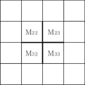
Figure 3. Four central edges

Fact 3. As in Fact 2, if both central edges of $M_{ij}$ have connection points, then $M_{ij}$ has 5 choices of mosaic tiles. Otherwise, it has 2 choices.

First we figure out $\mathbb{K}^{(4)}_{c}$ and find the number $d_{c}$. Since each central edge has 2 cases whether it has a connection point or not, we split into 16 cases whether each of four central edges has a connection point or not.

Among 16 cases, there is only one case where all four central edges have connection points. By Fact 3, every $M_{ij}$ has 5 choices, so we have $5^{4}$ different $4$-quasimosaics in $\mathbb{K}^{(4)}_{c}$. There are four cases where exactly three central edges have connection points. In each case two of $M_{ij}$’s have 5 choices and the other two have 2 choices, and so we have $5^{2}\cdot 2^{2}$ different $4$-quasimosaics. There are another four cases where only two perpendicular central edges have connection points. In each case only one of $M_{ij}$’s has 5 choices and the other three have 2 choices, and so we have $5\cdot 2^{3}$. In each of the rest seven cases, every $M_{ij}$ has 2 choices, so we have $2^{4}$. Thus we have the following;

$d_{c}=5^{4}+4\cdot 5^{2}\cdot 2^{2}+4\cdot 5\cdot 2^{3}+7\cdot 2^{4}=1297$.

Finally we are ready to finish the proof of Theorem 2. For each $4$-quasimosaic in $\mathbb{K}^{(4)}_{c}$, there are exactly two ways to fill mosaic tiles to be suitably connected at the rest twelve boundary $M_{ij}$’s. For, every tile has even numbered connection points, so the union of boundary edges of $M_{22}\cup M_{23}\cup M_{32}\cup M_{33}$ has even number of connection points. This implies that $D_{4}=2d_{c}$.

References

- [1] K. Hong, H. Lee, H. J. Lee and S. Oh, Small knot mosaics and partition matrices, J. Phys. A: Math. Theor. 47 (2014) 435201.
- [2] L. Kauffman, Quantum computing and the Jones polynomial, in Quantum Computation and Information, AMS CONM 305 (2002) 101–137.
- [3] T. Kuriya and O. Shehab, The Lomonaco-Kauffman conjecture, J. Knot Theory Ramifications 23 (2014) 1450003.
- [4] H. J. Lee, K. Hong, H. Lee and S. Oh, Mosaic number of knots, arXiv:1301.6041.
- [5] S. Lomonaco, Quantum Computation, Proc. Symposia Appl. Math. 58 (2002) 358 pp.
- [6] S. Lomonaco and L. Kauffman, Quantum knots, in Quantum Information and Computation II, Proc. SPIE (2004) 268–284.
- [7] S. Lomonaco and L. Kauffman, Quantum knots and mosaics, Quantum Inf. Process. 7 (2008) 85–115.
- [8] S. Lomonaco and L. Kauffman, Quantum knots and lattices, or a blueprint for quantum systems that do rope tricks, Proc. Symposia Appl. Math. 68 (2010) 209–276.
- [9] S. Lomonaco and L. Kauffman, Quantizing knots and beyond, in Quantum Information and Computation IX, Proc. SPIE 8057 (2011) 1–14.
- [10] S. Oh, Quantum knot mosaics and the growth constant, Preprint.
- [11] S. Oh, K. Hong, H. Lee and H. J. Lee, Quantum knots and the number of knot mosaics, Preprint.