Symmetries of Codeword Stabilized Quantum Codes

Abstract.

Symmetry is at the heart of coding theory. Codes with symmetry, especially cyclic codes, play an essential role in both theory and practical applications of classical error-correcting codes. Here we examine symmetry properties for codeword stabilized (CWS) quantum codes, which is the most general framework for constructing quantum error-correcting codes known to date. A CWS code $\mathcal{Q}$ can be represented by a self-dual additive code $\mathcal{S}$ and a classical code $\mathcal{C}$, i. e., $\mathcal{Q}=(\mathcal{S},\mathcal{C})$, however this representation is in general not unique. We show that for any CWS code $\mathcal{Q}$ with certain permutation symmetry, one can always find a self-dual additive code $\mathcal{S}$ with the same permutation symmetry as $\mathcal{Q}$ such that $\mathcal{Q}=(\mathcal{S},\mathcal{C})$. As many good CWS codes have been found by starting from a chosen $\mathcal{S}$, this ensures that when trying to find CWS codes with certain permutation symmetry, the choice of $\mathcal{S}$ with the same symmetry will suffice. A key step for this result is a new canonical representation for CWS codes, which is given in terms of a unique decomposition as union stabilizer codes. For CWS codes, so far mainly the standard form $(\mathcal{G},\mathcal{C})$ has been considered, where $\mathcal{G}$ is a graph state. We analyze the symmetry of the corresponding graph of $\mathcal{G}$, which in general cannot possess the same permutation symmetry as $\mathcal{Q}$. We show that it is indeed the case for the toric code on a square lattice with translational symmetry, even if its encoding graph can be chosen to be translational invariant.

1. Introduction

Coding theory is an important component of information theory having a long history dating back to Shannon’s seminal 1948 paper that laid the ground for information theory [21]. Coding theory is at the heart of reliable communication, where codes with symmetry, especially cyclic codes, such as the Reed-Solomon codes, are among the most widely used codes in practice [19].

In recent years, it has become evident that quantum communication and computation offer the possibility of secure and high rate information transmission, fast computational solution of certain important problems, and efficient physical simulation of quantum phenomena. However, quantum information processing depends on the identification of suitable quantum error-correcting codes (QECC) to make such processes and machines robust against faults due to decoherence, ubiquitous in quantum systems. Quantum coding theory has hence been extensively developed during the past 15 years [3, 9, 20].

Codeword stabilized (CWS) quantum codes are by far the most general construction of QECC [6]. A CWS code $\mathcal{Q}$ can be represented by a stabilizer state (i. e. a self-dual additive code) $\mathcal{S}$ and a classical code $\mathcal{C}$, i. e. $\mathcal{Q}=(\mathcal{S},\mathcal{C})$. When $\mathcal{C}$ is a linear code, the corresponding CWS code $\mathcal{Q}$ is actually a stabilizer code. Also, any CWS code is local Clifford equivalent to a standard form $(\mathcal{G},\mathcal{C})$, where $\mathcal{G}$ is a graph state [6].

The CWS construction encompasses stabilizer (additive) codes and all the known non-additive codes with good parameters. It also leads to many new codes with good parameters, or good algebraic/combinatorial properties, through both analytical and numerical methods. Alternative perspectives of CWS codes have also been analyzed, including the union stabilizer codes (USt) method [11, 12], and the codes based on graphs [18, 23]. Concatenated codes and their generalizations using CWS codes have been developed [1], and decoding methods for CWS codes have been studied as well [17].

Given all the evidence that the CWS framework is a powerful method to construct and analyze QECC, it remains unclear to what extent the stabilizer state $\mathcal{S}$ and the classical code $\mathcal{C}$ can represent the symmetry of the CWS code $\mathcal{Q}=(\mathcal{S},\mathcal{C})$ in general. Given the vital importance that the code symmetry plays in coding theory, this understanding becomes crucial since if such a correspondence exists, it can provide practical methods for constructing CWS codes with desired symmetry from $\mathcal{S}$ and/or $\mathcal{C}$ with corresponding symmetry.

Unfortunately, there is no immediate clue what answer one can hope for. First of all, the representation $\mathcal{Q}=(\mathcal{S},\mathcal{C})$ is not unique. So for a given CWS code $\mathcal{Q}$, there might be some stabilizer states $\mathcal{S}$ and/or classical codes $\mathcal{C}$ which are more symmetric than others. Perhaps the best known example is the CWS representation for the five-qubit code $\mathcal{Q}_{5}$, where in the ideal case $\mathcal{S}$ can be chosen as a graph state corresponding to the pentagon graph, and the $\mathcal{C}$ is chosen as the repetition code $\{00000,11111\}$. In this case, both $\mathcal{S}$ and $\mathcal{C}$ nicely represent the cyclic symmetry of the five-qubit code.

However, there are known ‘bad cases’, too. One example is the seven-qubit Steane code $\mathcal{Q}_{7}$, where although the code itself is cyclic, one cannot find any $\mathcal{S}$ corresponding to a cyclic graph, even if local Clifford operations are allowed [10]. Nonetheless, we know that the stabilizer group for this code $\mathcal{Q}_{7}$ is invariant under cyclic shifts, and the logical $Z$ operator can be chosen as $Z_{L}=Z^{\otimes 7}$, therefore the logical $|0\rangle_{L}$ can be chosen as a cyclic stabilizer code. This is to say, there exists a representation for $\mathcal{Q}_{7}=(\mathcal{S},\mathcal{C})$ such that $\mathcal{S}$ is cyclic. In general it remains unclear under which conditions a representation for cyclic CWS code with a cyclic stabilizer state $\mathcal{S}$ exists.

In this work, we address the symmetry properties of CWS codes. We are interested in the permutation symmetry of CWS codes, which includes the important category of cyclic codes. Our main question is, to which extent can the representation $(\mathcal{S},\mathcal{C})$ and the standard form $(\mathcal{G},\mathcal{C})$ reflect the symmetry of the corresponding CWS code $\mathcal{Q}$. We show that for any CWS code $\mathcal{Q}$ with permutation symmetry, one can always find a stabilizer state $\mathcal{S}$ with the same permutation symmetry as $\mathcal{Q}$ such that $\mathcal{Q}=(\mathcal{S},\mathcal{C})$. As many good CWS codes are found by starting from a chosen $\mathcal{S}$, this ensures that when trying to find CWS codes with certain permutation symmetry, the choice of $\mathcal{S}$ with the same symmetry will suffice. A key step to reach this main result is to obtain a canonical representation for CWS codes, which is in terms of a unique decomposition as union stabilizer codes.

We know that for the standard form of CWS codes using graph states, it is not always possible to find a graph with the same permutation symmetry. This is partially due to the fact that the local Clifford operation transforming the CWS code into the standard form may break the permutation symmetry of the original code. Also, the graphs usually can only represent the symmetry of the stabilizer generators of the stabilizer state, but not the symmetry of the stabilizer state in general. We show that this is indeed the case for the toric code on a two-dimensional square lattice with translational symmetry, even if its encoding graph can be chosen to be translational invariant.

However, we show that the converse always holds, i. e., any graph $\mathcal{G}$ and classical code $\mathcal{C}$ with certain permutation symmetry yields a CWS code $\mathcal{Q}=(\mathcal{G},\mathcal{C})$ with the same symmetry.

2. Preliminaries

The single-qudit (generalized) Pauli group is generated by the operators $X$ and $Z$ acting on the qudit Hilbert space ${\mathbb{C}}^{p}$, satisfying $ZX=\omega XZ$, where $\omega=\omega_{p}=\exp{2i\pi/p}$. For simplicity, throughout the paper, we assume that $p$ is a prime, although our results naturally extend to prime powers. Denote the computational basis of ${\mathbb{C}}^{p}$ by $\{|j\rangle\colon j=0,1,\ldots,p-1\}$. Then, without loss of generality, we can fix the operators $X$ and $Z$ such that $X|j\rangle=|j+1\rangle$ and $Z|j\rangle=\omega^{j}|j\rangle$, respectively. Let $I$ be the identity operator. The set $\{X^{a}Z^{b}\colon a,b=0,\ldots,p-1\}$ of $p^{2}$ operators forms a so-called nice unitary error basis which is a particular basis for the vector space of $p\times p$ matrices [15, 16].

The $n$-qudit Pauli group ${\mathcal{P}}_{n}$ consists of all local operators of the form $\mathchoice{\mbox{\boldmath{$\displaystyle M$}}}{\mbox{\boldmath{$\textstyle M$}}}{\mbox{\boldmath{$\scriptstyle M$}}}{\mbox{\boldmath{$\scriptscriptstyle M$}}}=\alpha_{\mathchoice{\mbox{\boldmath{$\displaystyle M$}}}{\mbox{\boldmath{$\textstyle M$}}}{\mbox{\boldmath{$\scriptstyle M$}}}{\mbox{\boldmath{$\scriptscriptstyle M$}}}}M_{1}\otimes\dots\otimes M_{n}$, where $\alpha_{\mathchoice{\mbox{\boldmath{$\displaystyle M$}}}{\mbox{\boldmath{$\textstyle M$}}}{\mbox{\boldmath{$\scriptstyle M$}}}{\mbox{\boldmath{$\scriptscriptstyle M$}}}}=\omega^{k}$ for some integer $k$ is an overall phase factor, and $M_{i}=X_{i}^{a}Z_{i}^{b}$ for some $a,b\in\{0,1,\ldots,p-1\}$, is an element of the single-qudit Pauli group of qudit $i$. We can write $\textstyle M$ as $\alpha_{\mathchoice{\mbox{\boldmath{$\displaystyle M$}}}{\mbox{\boldmath{$\textstyle M$}}}{\mbox{\boldmath{$\scriptstyle M$}}}{\mbox{\boldmath{$\scriptscriptstyle M$}}}}(M_{1})_{1}(M_{2})_{2}\dots(M_{n})_{n}$ or $\alpha_{\mathchoice{\mbox{\boldmath{$\displaystyle M$}}}{\mbox{\boldmath{$\textstyle M$}}}{\mbox{\boldmath{$\scriptstyle M$}}}{\mbox{\boldmath{$\scriptscriptstyle M$}}}}M_{1}M_{2}\dots M_{n}$ when it is clear what the qudit labels are. The weight of an operator $\textstyle M$ is the number of tensor factors $M_{i}$ that differ from identity.

The $n$-qudit Clifford group ${\mathcal{L}}_{n}$ is the group of $p^{n}\times p^{n}$ unitary matrices that map ${\mathcal{P}}_{n}$ to itself under conjugation. The $n$-qudit local Clifford group is a subgroup in ${\mathcal{L}}_{n}$ containing elements of the form $M_{1}\otimes\dots\otimes M_{n}$, where each $M_{i}$ is a single qudit Clifford operation, i. e., $M_{i}\in{\mathcal{L}}_{1}$.

A stabilizer group $\mathcal{S}$ in the Pauli group ${\mathcal{P}}_{n}$ is defined as an abelian subgroup of ${\mathcal{P}}_{n}$ which does not contain $\omega I$. A stabilizer consists of $p^{m}$ Pauli operators for some $m\leq n$. As the operators in a stabilizer commute with each other, they can be simultaneously diagonalized. The common eigenspace of eigenvalue $1$ is a stabilizer quantum code $\mathcal{Q}=(\!(n,K,d)\!)_{p}$ with length $n$, dimension $K=p^{n-m}$, and minimum distance $d$. The projection $P_{\mathcal{Q}}$ onto the code $\mathcal{Q}$ can be expressed as

$$P_{\mathcal{Q}}=\frac{1}{|\mathcal{S}|}\sum_{\mathchoice{\mbox{\boldmath{$\displaystyle M$}}}{\mbox{\boldmath{$\textstyle M$}}}{\mbox{\boldmath{$\scriptstyle M$}}}{\mbox{\boldmath{$\scriptscriptstyle M$}}}\in\mathcal{S}}\mathchoice{\mbox{\boldmath{$\displaystyle M$}}}{\mbox{\boldmath{$\textstyle M$}}}{\mbox{\boldmath{$\scriptstyle M$}}}{\mbox{\boldmath{$\scriptscriptstyle M$}}}.$$ (1)

The centralizer $C(\mathcal{S})$ of the stabilizer $\mathcal{S}$ is given by the elements in ${\mathcal{P}}_{n}$ which commute with all elements in $\mathcal{S}$. For $m<n$, the minimum distance $d$ of the code $\mathcal{Q}$ is the minimum weight of all elements in $C(\mathcal{S})\setminus\mathcal{S}$.

If $m=n$, then there exists a unique $n$-qudit state $|\psi\rangle$ such that $\mathchoice{\mbox{\boldmath{$\displaystyle M$}}}{\mbox{\boldmath{$\textstyle M$}}}{\mbox{\boldmath{$\scriptstyle M$}}}{\mbox{\boldmath{$\scriptscriptstyle M$}}}|\psi\rangle=|\psi\rangle$ for every $\mathchoice{\mbox{\boldmath{$\displaystyle M$}}}{\mbox{\boldmath{$\textstyle M$}}}{\mbox{\boldmath{$\scriptstyle M$}}}{\mbox{\boldmath{$\scriptscriptstyle M$}}}\in{\mathcal{S}}$. Such a state $|\psi\rangle$ is called a stabilizer state, and the group ${\mathcal{S}}={\mathcal{S}}(|\psi\rangle)$ is called the stabilizer of $|\psi\rangle$. A stabilizer state can also be viewed as a self-dual code over the finite field ${\mathbb{F}}_{p^{2}}$ under the trace inner product [7]. For a stabilizer state, the minimum distance is defined as the minimum weight of the non-trivial elements in $\mathcal{S}(|\psi\rangle)$ [7].

A union stabilizer (USt) code of length $n$ is characterized by a stabilizer code with stabilizer $\mathcal{S}=\langle\mathchoice{\mbox{\boldmath{$\displaystyle g$}}}{\mbox{\boldmath{$\textstyle g$}}}{\mbox{\boldmath{$\scriptstyle g$}}}{\mbox{\boldmath{$\scriptscriptstyle g$}}}_{1},\mathchoice{\mbox{\boldmath{$\displaystyle g$}}}{\mbox{\boldmath{$\textstyle g$}}}{\mbox{\boldmath{$\scriptstyle g$}}}{\mbox{\boldmath{$\scriptscriptstyle g$}}}_{2},\ldots,\mathchoice{\mbox{\boldmath{$\displaystyle g$}}}{\mbox{\boldmath{$\textstyle g$}}}{\mbox{\boldmath{$\scriptstyle g$}}}{\mbox{\boldmath{$\scriptscriptstyle g$}}}_{m}\rangle$, where $\mathchoice{\mbox{\boldmath{$\displaystyle g$}}}{\mbox{\boldmath{$\textstyle g$}}}{\mbox{\boldmath{$\scriptstyle g$}}}{\mbox{\boldmath{$\scriptscriptstyle g$}}}_{1},\mathchoice{\mbox{\boldmath{$\displaystyle g$}}}{\mbox{\boldmath{$\textstyle g$}}}{\mbox{\boldmath{$\scriptstyle g$}}}{\mbox{\boldmath{$\scriptscriptstyle g$}}}_{2},\ldots,\mathchoice{\mbox{\boldmath{$\displaystyle g$}}}{\mbox{\boldmath{$\textstyle g$}}}{\mbox{\boldmath{$\scriptstyle g$}}}{\mbox{\boldmath{$\scriptscriptstyle g$}}}_{m}$ are $m$ independent generators, and a classical code $\mathcal{C}$ over ${\mathbb{F}}_{p}$ of length $m$. Note that for a given $\mathcal{S}$, the choice of the $m$ generators $\mathchoice{\mbox{\boldmath{$\displaystyle g$}}}{\mbox{\boldmath{$\textstyle g$}}}{\mbox{\boldmath{$\scriptstyle g$}}}{\mbox{\boldmath{$\scriptscriptstyle g$}}}_{j}$ is not unique. Now for a classical code $\mathcal{C}$ of length $m$ with $K$ codewords, for each codeword $\mathbf{c}=(c_{1},c_{2},\ldots,c_{m})\in\mathcal{C}$, the corresponding quantum code is given by the subspace $V_{\mathchoice{\mbox{\boldmath{$\displaystyle c$}}}{\mbox{\boldmath{$\textstyle c$}}}{\mbox{\boldmath{$\scriptstyle c$}}}{\mbox{\boldmath{$\scriptscriptstyle c$}}}}$ stabilized by $\omega^{c_{1}}\mathchoice{\mbox{\boldmath{$\displaystyle g$}}}{\mbox{\boldmath{$\textstyle g$}}}{\mbox{\boldmath{$\scriptstyle g$}}}{\mbox{\boldmath{$\scriptscriptstyle g$}}}_{1}$, $\omega^{c_{2}}\mathchoice{\mbox{\boldmath{$\displaystyle g$}}}{\mbox{\boldmath{$\textstyle g$}}}{\mbox{\boldmath{$\scriptstyle g$}}}{\mbox{\boldmath{$\scriptscriptstyle g$}}}_{2}$, …, $\omega^{c_{m}}\mathchoice{\mbox{\boldmath{$\displaystyle g$}}}{\mbox{\boldmath{$\textstyle g$}}}{\mbox{\boldmath{$\scriptstyle g$}}}{\mbox{\boldmath{$\scriptscriptstyle g$}}}_{m}$. Note that for ${\mathchoice{\mbox{\boldmath{$\displaystyle c$}}}{\mbox{\boldmath{$\textstyle c$}}}{\mbox{\boldmath{$\scriptstyle c$}}}{\mbox{\boldmath{$\scriptscriptstyle c$}}}}\neq{\mathchoice{\mbox{\boldmath{$\displaystyle c$}}}{\mbox{\boldmath{$\textstyle c$}}}{\mbox{\boldmath{$\scriptstyle c$}}}{\mbox{\boldmath{$\scriptscriptstyle c$}}}}^{\prime}\in\mathcal{C}$, the subspaces $V_{\mathchoice{\mbox{\boldmath{$\displaystyle c$}}}{\mbox{\boldmath{$\textstyle c$}}}{\mbox{\boldmath{$\scriptstyle c$}}}{\mbox{\boldmath{$\scriptscriptstyle c$}}}}$ and $V_{{\mathchoice{\mbox{\boldmath{$\displaystyle c$}}}{\mbox{\boldmath{$\textstyle c$}}}{\mbox{\boldmath{$\scriptstyle c$}}}{\mbox{\boldmath{$\scriptscriptstyle c$}}}}^{\prime}}$ are mutually orthogonal. The corresponding USt code is then given by the subspace $\bigoplus_{\mathchoice{\mbox{\boldmath{$\displaystyle c$}}}{\mbox{\boldmath{$\textstyle c$}}}{\mbox{\boldmath{$\scriptstyle c$}}}{\mbox{\boldmath{$\scriptscriptstyle c$}}}}V_{\mathchoice{\mbox{\boldmath{$\displaystyle c$}}}{\mbox{\boldmath{$\textstyle c$}}}{\mbox{\boldmath{$\scriptstyle c$}}}{\mbox{\boldmath{$\scriptscriptstyle c$}}}}$.

Therefore, the combination of $\mathcal{S}$ (more precisely, the generators of $\mathcal{S}$) and $\cal{C}$ gives an $(\!(n,2^{n-m}K)\!)_{p}$ USt quantum code $\mathcal{Q}$. Hence we denote a USt code $\cal{Q}$ by $\cal{Q}=(\cal{S},\cal{C})$. The projection onto $\mathcal{Q}$ can be expressed as

$$P_{\mathcal{Q}}=\sum_{\mathchoice{\mbox{\boldmath{$\displaystyle c$}}}{\mbox{\boldmath{$\textstyle c$}}}{\mbox{\boldmath{$\scriptstyle c$}}}{\mbox{\boldmath{$\scriptscriptstyle c$}}}\in\mathcal{C}}\frac{1}{p^{m}}\sum_{\mathchoice{\mbox{\boldmath{$\displaystyle y$}}}{\mbox{\boldmath{$\textstyle y$}}}{\mbox{\boldmath{$\scriptstyle y$}}}{\mbox{\boldmath{$\scriptscriptstyle y$}}}\in{\mathbb{F}}_{p}^{m}}\omega^{\mathchoice{\mbox{\boldmath{$\displaystyle c$}}}{\mbox{\boldmath{$\textstyle c$}}}{\mbox{\boldmath{$\scriptstyle c$}}}{\mbox{\boldmath{$\scriptscriptstyle c$}}}\cdot\mathchoice{\mbox{\boldmath{$\displaystyle y$}}}{\mbox{\boldmath{$\textstyle y$}}}{\mbox{\boldmath{$\scriptstyle y$}}}{\mbox{\boldmath{$\scriptscriptstyle y$}}}}\mathchoice{\mbox{\boldmath{$\displaystyle g$}}}{\mbox{\boldmath{$\textstyle g$}}}{\mbox{\boldmath{$\scriptstyle g$}}}{\mbox{\boldmath{$\scriptscriptstyle g$}}}_{1}^{y_{1}}\dots\mathchoice{\mbox{\boldmath{$\displaystyle g$}}}{\mbox{\boldmath{$\textstyle g$}}}{\mbox{\boldmath{$\scriptstyle g$}}}{\mbox{\boldmath{$\scriptscriptstyle g$}}}_{m}^{y_{m}},$$ (2)

where we identify the elements $y_{i}$ of the finite field with integers modulo $p$.

A CWS code $\cal{Q}$ of length $n$ is a USt code with $m=n$. That is, it is characterized by a stabilizer state with stabilizer $\mathcal{S}$ and a classical code $\mathcal{C}$ of length $n$. For a CWS code $\cal{Q}$ given by $\cal{Q}=(\cal{S},\cal{C})$, the stabilizer $\cal{S}$ always corresponds to a unique stabilizer state. We will then refer to $\mathcal{S}$ as the stabilizer state when no confusion arises.

For a CWS code, the projection $P_{\cal{Q}}$ onto the code space is given by

$$P_{\mathcal{Q}}=\sum_{\mathchoice{\mbox{\boldmath{$\displaystyle t$}}}{\mbox{\boldmath{$\textstyle t$}}}{\mbox{\boldmath{$\scriptstyle t$}}}{\mbox{\boldmath{$\scriptscriptstyle t$}}}\in{\mathcal{C}}}\frac{1}{p^{n}}\sum_{\mathchoice{\mbox{\boldmath{$\displaystyle x$}}}{\mbox{\boldmath{$\textstyle x$}}}{\mbox{\boldmath{$\scriptstyle x$}}}{\mbox{\boldmath{$\scriptscriptstyle x$}}}\in{\mathbb{F}}_{p}^{n}}\omega^{\mathchoice{\mbox{\boldmath{$\displaystyle t$}}}{\mbox{\boldmath{$\textstyle t$}}}{\mbox{\boldmath{$\scriptstyle t$}}}{\mbox{\boldmath{$\scriptscriptstyle t$}}}\cdot\mathchoice{\mbox{\boldmath{$\displaystyle x$}}}{\mbox{\boldmath{$\textstyle x$}}}{\mbox{\boldmath{$\scriptstyle x$}}}{\mbox{\boldmath{$\scriptscriptstyle x$}}}}\mathchoice{\mbox{\boldmath{$\displaystyle g$}}}{\mbox{\boldmath{$\textstyle g$}}}{\mbox{\boldmath{$\scriptstyle g$}}}{\mbox{\boldmath{$\scriptscriptstyle g$}}}_{1}^{x_{1}}\dots\mathchoice{\mbox{\boldmath{$\displaystyle g$}}}{\mbox{\boldmath{$\textstyle g$}}}{\mbox{\boldmath{$\scriptstyle g$}}}{\mbox{\boldmath{$\scriptscriptstyle g$}}}_{n}^{x_{n}},$$ (3)

where we again identify the elements $x_{i}$ of the finite field with integers modulo $p$.

A CWS code has a permutation symmetry $\sigma$ if

$$P_{\mathcal{Q}}^{\sigma}=P_{\mathcal{Q}},$$ (4)

where $P_{\mathcal{Q}}^{\sigma}$ is the projection onto the space obtained by permuting the qudits of the code $\mathcal{Q}$ according to $\sigma$.

3. Canonical form of CWS codes

For a given a CWS code $\mathcal{Q}=(\mathcal{S},\mathcal{C})$, there might exist another stabilizer state $\mathcal{S}^{\prime}$ and another classical code $\mathcal{C}^{\prime}$ such that $\mathcal{Q}=(\mathcal{S}^{\prime},\mathcal{C}^{\prime})$. In other words, the representation of a CWS code by the stabilizer state $\mathcal{S}$ and the classical code $\mathcal{C}$ is non-unique.

In order to discuss the relationship between the symmetry of the CWS code $\mathcal{Q}$ and that of the stabilizer state $\mathcal{S}$, we first need to explore the relationship between the different representations of $\mathcal{Q}$ (i. e., the relationship between $\mathcal{S}$ and $\mathcal{S}^{\prime}$, as well as the relationship between $\mathcal{C}$ and $\mathcal{C}^{\prime}$).

Let us start by recalling that a stabilizer code can be viewed as a CWS code where the classical code is a linear code [6]. A simple way to see this is that for a given stabilizer code $\mathcal{Q}_{s}$ with stabilizer generated by $\mathcal{S}=\langle\mathchoice{\mbox{\boldmath{$\displaystyle g$}}}{\mbox{\boldmath{$\textstyle g$}}}{\mbox{\boldmath{$\scriptstyle g$}}}{\mbox{\boldmath{$\scriptscriptstyle g$}}}_{1},\mathchoice{\mbox{\boldmath{$\displaystyle g$}}}{\mbox{\boldmath{$\textstyle g$}}}{\mbox{\boldmath{$\scriptstyle g$}}}{\mbox{\boldmath{$\scriptscriptstyle g$}}}_{2},\ldots,\mathchoice{\mbox{\boldmath{$\displaystyle g$}}}{\mbox{\boldmath{$\textstyle g$}}}{\mbox{\boldmath{$\scriptstyle g$}}}{\mbox{\boldmath{$\scriptscriptstyle g$}}}_{m}\rangle$, which is a code of dimension $p^{n-m}$, we can choose the larger stabilizer $\mathcal{S}^{\prime}=\langle\mathchoice{\mbox{\boldmath{$\displaystyle g$}}}{\mbox{\boldmath{$\textstyle g$}}}{\mbox{\boldmath{$\scriptstyle g$}}}{\mbox{\boldmath{$\scriptscriptstyle g$}}}_{1},\mathchoice{\mbox{\boldmath{$\displaystyle g$}}}{\mbox{\boldmath{$\textstyle g$}}}{\mbox{\boldmath{$\scriptstyle g$}}}{\mbox{\boldmath{$\scriptscriptstyle g$}}}_{2},\ldots,\mathchoice{\mbox{\boldmath{$\displaystyle g$}}}{\mbox{\boldmath{$\textstyle g$}}}{\mbox{\boldmath{$\scriptstyle g$}}}{\mbox{\boldmath{$\scriptscriptstyle g$}}}_{m},\bar{Z}_{1},\ldots,\bar{Z}_{n-m}\rangle$, where $\bar{Z}_{1},\ldots,\bar{Z}_{n-m}\in C(\mathcal{S})$ mutually commute. Now choose the classical code $\mathcal{C}^{\prime}=\bigl{\{}(0,\ldots,0,x_{m+1},\ldots,x_{n})\colon x_{j}\in\{0,\ldots,p-1\}\bigr{\}}$ of length $n$ with $p^{n-m}$ codewords, where the first $m$ coordinates of each codeword are zero. Then we have $\mathcal{Q}_{s}=(\mathcal{S}^{\prime},\mathcal{C}^{\prime})$, i. e., the stabilizer code $\mathcal{Q}_{s}$ can then be viewed as a CWS code with stabilizer state $\mathcal{S}^{\prime}$ and classical code $\mathcal{C}^{\prime}$. However, note that the choice of $\mathcal{S}^{\prime}$ (and hence $\mathcal{C}^{\prime}$) is non-unique, as in particular the choice of $\bar{Z}_{1},\ldots,\bar{Z}_{n-s}\in C(\mathcal{S})$ is non-unique.

Example 3.1.

As an example, consider the five-qubit code with stabilizer

$$\mathchoice{\mbox{\boldmath{$\displaystyle g$}}}{\mbox{\boldmath{$\textstyle g$}}}{\mbox{\boldmath{$\scriptstyle g$}}}{\mbox{\boldmath{$\scriptscriptstyle g$}}}_{1}=XZZXI,\quad\mathchoice{\mbox{\boldmath{$\displaystyle g$}}}{\mbox{\boldmath{$\textstyle g$}}}{\mbox{\boldmath{$\scriptstyle g$}}}{\mbox{\boldmath{$\scriptscriptstyle g$}}}_{2}=IXZZX,\quad\mathchoice{\mbox{\boldmath{$\displaystyle g$}}}{\mbox{\boldmath{$\textstyle g$}}}{\mbox{\boldmath{$\scriptstyle g$}}}{\mbox{\boldmath{$\scriptscriptstyle g$}}}_{3}=XIXZZ,\quad\mathchoice{\mbox{\boldmath{$\displaystyle g$}}}{\mbox{\boldmath{$\textstyle g$}}}{\mbox{\boldmath{$\scriptstyle g$}}}{\mbox{\boldmath{$\scriptscriptstyle g$}}}_{4}=ZXIXZ.$$ (5)

In the CWS picture, the stabilizer state can be chosen as

$$\mathcal{S}=\langle\mathchoice{\mbox{\boldmath{$\displaystyle g$}}}{\mbox{\boldmath{$\textstyle g$}}}{\mbox{\boldmath{$\scriptstyle g$}}}{\mbox{\boldmath{$\scriptscriptstyle g$}}}_{1},\mathchoice{\mbox{\boldmath{$\displaystyle g$}}}{\mbox{\boldmath{$\textstyle g$}}}{\mbox{\boldmath{$\scriptstyle g$}}}{\mbox{\boldmath{$\scriptscriptstyle g$}}}_{2},\mathchoice{\mbox{\boldmath{$\displaystyle g$}}}{\mbox{\boldmath{$\textstyle g$}}}{\mbox{\boldmath{$\scriptstyle g$}}}{\mbox{\boldmath{$\scriptscriptstyle g$}}}_{3},\mathchoice{\mbox{\boldmath{$\displaystyle g$}}}{\mbox{\boldmath{$\textstyle g$}}}{\mbox{\boldmath{$\scriptstyle g$}}}{\mbox{\boldmath{$\scriptscriptstyle g$}}}_{4},\mathchoice{\mbox{\boldmath{$\displaystyle Z$}}}{\mbox{\boldmath{$\textstyle Z$}}}{\mbox{\boldmath{$\scriptstyle Z$}}}{\mbox{\boldmath{$\scriptscriptstyle Z$}}}_{L}\rangle,$$ (6)

where $\mathchoice{\mbox{\boldmath{$\displaystyle Z$}}}{\mbox{\boldmath{$\textstyle Z$}}}{\mbox{\boldmath{$\scriptstyle Z$}}}{\mbox{\boldmath{$\scriptscriptstyle Z$}}}_{L}=Z^{\otimes 5}$ is the logical $Z$ operator. Alternatively, one can choose the stabilizer state

$$\mathcal{S}^{\prime}=\langle\mathchoice{\mbox{\boldmath{$\displaystyle g$}}}{\mbox{\boldmath{$\textstyle g$}}}{\mbox{\boldmath{$\scriptstyle g$}}}{\mbox{\boldmath{$\scriptscriptstyle g$}}}_{1},\mathchoice{\mbox{\boldmath{$\displaystyle g$}}}{\mbox{\boldmath{$\textstyle g$}}}{\mbox{\boldmath{$\scriptstyle g$}}}{\mbox{\boldmath{$\scriptscriptstyle g$}}}_{2},\mathchoice{\mbox{\boldmath{$\displaystyle g$}}}{\mbox{\boldmath{$\textstyle g$}}}{\mbox{\boldmath{$\scriptstyle g$}}}{\mbox{\boldmath{$\scriptscriptstyle g$}}}_{3},\mathchoice{\mbox{\boldmath{$\displaystyle g$}}}{\mbox{\boldmath{$\textstyle g$}}}{\mbox{\boldmath{$\scriptstyle g$}}}{\mbox{\boldmath{$\scriptscriptstyle g$}}}_{4},\mathchoice{\mbox{\boldmath{$\displaystyle X$}}}{\mbox{\boldmath{$\textstyle X$}}}{\mbox{\boldmath{$\scriptstyle X$}}}{\mbox{\boldmath{$\scriptscriptstyle X$}}}_{L}\rangle,$$ (7)

where $\mathchoice{\mbox{\boldmath{$\displaystyle X$}}}{\mbox{\boldmath{$\textstyle X$}}}{\mbox{\boldmath{$\scriptstyle X$}}}{\mbox{\boldmath{$\scriptscriptstyle X$}}}_{L}=X^{\otimes 5}$ is the logical $X$ operator. For both $S$ and $S^{\prime}$, the classical code can be chosen as $\mathcal{C}=\{00000,00001\}$.

Similarly, a USt code $(\mathcal{S},\mathcal{C})$ can be viewed as a CWS code $(\mathcal{S}^{\prime},\mathcal{C}^{\prime})$ with the classical code $\mathcal{C}^{\prime}$ of length $n$ possessing some coset structure, i. e., $\mathcal{C}^{\prime}=\bigcup_{\mathchoice{\mbox{\boldmath{$\displaystyle t$}}}{\mbox{\boldmath{$\textstyle t$}}}{\mbox{\boldmath{$\scriptstyle t$}}}{\mbox{\boldmath{$\scriptscriptstyle t$}}}_{i}\in\tilde{\mathcal{C}}}\mathcal{C}_{0}+\mathchoice{\mbox{\boldmath{$\displaystyle t$}}}{\mbox{\boldmath{$\textstyle t$}}}{\mbox{\boldmath{$\scriptstyle t$}}}{\mbox{\boldmath{$\scriptscriptstyle t$}}}_{i}$, where $\mathcal{C}_{0}$ is a linear code. This linear code $\mathcal{C}_{0}$ of length $n$ can be readily chosen as the classical code for the CWS representation of the stabilizer code $\mathcal{S}$. The code $\tilde{\mathcal{C}}$ of length $n$ can be derived from $\mathcal{C}$ of length $m$ by appending $n-m$ zero coordinates. However, again, the choices of $\mathcal{S}^{\prime}$ and $\mathcal{C}^{\prime}$ are non-unique.

In the general situation, we have some freedom in choosing the stabilizer state when representing a stabilizer code or a USt code in the CWS framework. Consequently, for a given CWS code $\mathcal{Q}$, there are also many different ways to write it in terms of a USt code in general. We will show, however, that we can always obtain a unique stabilizer $\mathcal{S}$, when expressing a given CWS code as a USt code. The following theorem gives a canonical form for any CWS code.

Theorem 3.2.

Every CWS code has a unique representation as a union stabilizer code.

Proof 3.3.

To prove this theorem, we will need some lemmas.

Lemma 3.4 (translational invariant codes).

Let $\mathcal{C}\subset{\mathbb{F}}_{p}^{n}$ be a code over ${\mathbb{F}}_{p}$ with $|\mathcal{C}|=M$ and assume that for some non-zero $\mathchoice{\mbox{\boldmath{$\displaystyle s$}}}{\mbox{\boldmath{$\textstyle s$}}}{\mbox{\boldmath{$\scriptstyle s$}}}{\mbox{\boldmath{$\scriptscriptstyle s$}}}\in{\mathbb{F}}_{p}^{n}$ we have $\mathcal{C}=\mathcal{C}+\mathchoice{\mbox{\boldmath{$\displaystyle s$}}}{\mbox{\boldmath{$\textstyle s$}}}{\mbox{\boldmath{$\scriptstyle s$}}}{\mbox{\boldmath{$\scriptscriptstyle s$}}}$, i. e., the code is invariant with respect to translation by $\textstyle s$. Then $\mathcal{C}$ can be written as a disjoint union of cosets of the one-dimensional space $\mathcal{C}_{0}=\langle\mathchoice{\mbox{\boldmath{$\displaystyle s$}}}{\mbox{\boldmath{$\textstyle s$}}}{\mbox{\boldmath{$\scriptstyle s$}}}{\mbox{\boldmath{$\scriptscriptstyle s$}}}\rangle$ generated by $\textstyle s$, i. e.,

$$\mathcal{C}=\bigcup_{\mathchoice{\mbox{\boldmath{$\displaystyle t$}}}{\mbox{\boldmath{$\textstyle t$}}}{\mbox{\boldmath{$\scriptstyle t$}}}{\mbox{\boldmath{$\scriptscriptstyle t$}}}_{i}\in\mathcal{C}^{\prime}}\mathcal{C}_{0}+\mathchoice{\mbox{\boldmath{$\displaystyle t$}}}{\mbox{\boldmath{$\textstyle t$}}}{\mbox{\boldmath{$\scriptstyle t$}}}{\mbox{\boldmath{$\scriptscriptstyle t$}}}_{i},$$

where $\mathcal{C}^{\prime}\subset{\mathbb{F}}_{p}^{n}$ with $|\mathcal{C}^{\prime}|=M/p$.

Proof 3.5.

By assumption, for every $\mathchoice{\mbox{\boldmath{$\displaystyle x$}}}{\mbox{\boldmath{$\textstyle x$}}}{\mbox{\boldmath{$\scriptstyle x$}}}{\mbox{\boldmath{$\scriptscriptstyle x$}}}\in\mathcal{C}$, the vector $\mathchoice{\mbox{\boldmath{$\displaystyle x$}}}{\mbox{\boldmath{$\textstyle x$}}}{\mbox{\boldmath{$\scriptstyle x$}}}{\mbox{\boldmath{$\scriptscriptstyle x$}}}+\mathchoice{\mbox{\boldmath{$\displaystyle s$}}}{\mbox{\boldmath{$\textstyle s$}}}{\mbox{\boldmath{$\scriptstyle s$}}}{\mbox{\boldmath{$\scriptscriptstyle s$}}}$ is in the code as well. Hence we can arrange the elements of $\mathcal{C}$ as follows:

$$\begin{array}[]{r|ccccc}\mathcal{C}^{\prime}&\mathchoice{\mbox{\boldmath{$\displaystyle t$}}}{\mbox{\boldmath{$\textstyle t$}}}{\mbox{\boldmath{$\scriptstyle t$}}}{\mbox{\boldmath{$\scriptscriptstyle t$}}}_{1}&\mathchoice{\mbox{\boldmath{$\displaystyle t$}}}{\mbox{\boldmath{$\textstyle t$}}}{\mbox{\boldmath{$\scriptstyle t$}}}{\mbox{\boldmath{$\scriptscriptstyle t$}}}_{2}&\ldots&\mathchoice{\mbox{\boldmath{$\displaystyle t$}}}{\mbox{\boldmath{$\textstyle t$}}}{\mbox{\boldmath{$\scriptstyle t$}}}{\mbox{\boldmath{$\scriptscriptstyle t$}}}_{M/p}\\ \hline\cr\mathcal{C}^{\prime}+\mathchoice{\mbox{\boldmath{$\displaystyle s$}}}{\mbox{\boldmath{$\textstyle s$}}}{\mbox{\boldmath{$\scriptstyle s$}}}{\mbox{\boldmath{$\scriptscriptstyle s$}}}&\mathchoice{\mbox{\boldmath{$\displaystyle t$}}}{\mbox{\boldmath{$\textstyle t$}}}{\mbox{\boldmath{$\scriptstyle t$}}}{\mbox{\boldmath{$\scriptscriptstyle t$}}}_{1}+\mathchoice{\mbox{\boldmath{$\displaystyle s$}}}{\mbox{\boldmath{$\textstyle s$}}}{\mbox{\boldmath{$\scriptstyle s$}}}{\mbox{\boldmath{$\scriptscriptstyle s$}}}&\mathchoice{\mbox{\boldmath{$\displaystyle t$}}}{\mbox{\boldmath{$\textstyle t$}}}{\mbox{\boldmath{$\scriptstyle t$}}}{\mbox{\boldmath{$\scriptscriptstyle t$}}}_{2}+\mathchoice{\mbox{\boldmath{$\displaystyle s$}}}{\mbox{\boldmath{$\textstyle s$}}}{\mbox{\boldmath{$\scriptstyle s$}}}{\mbox{\boldmath{$\scriptscriptstyle s$}}}&\ldots&\mathchoice{\mbox{\boldmath{$\displaystyle t$}}}{\mbox{\boldmath{$\textstyle t$}}}{\mbox{\boldmath{$\scriptstyle t$}}}{\mbox{\boldmath{$\scriptscriptstyle t$}}}_{M/p}+\mathchoice{\mbox{\boldmath{$\displaystyle s$}}}{\mbox{\boldmath{$\textstyle s$}}}{\mbox{\boldmath{$\scriptstyle s$}}}{\mbox{\boldmath{$\scriptscriptstyle s$}}}\\ \mathcal{C}^{\prime}+2\mathchoice{\mbox{\boldmath{$\displaystyle s$}}}{\mbox{\boldmath{$\textstyle s$}}}{\mbox{\boldmath{$\scriptstyle s$}}}{\mbox{\boldmath{$\scriptscriptstyle s$}}}&\mathchoice{\mbox{\boldmath{$\displaystyle t$}}}{\mbox{\boldmath{$\textstyle t$}}}{\mbox{\boldmath{$\scriptstyle t$}}}{\mbox{\boldmath{$\scriptscriptstyle t$}}}_{1}+2\mathchoice{\mbox{\boldmath{$\displaystyle s$}}}{\mbox{\boldmath{$\textstyle s$}}}{\mbox{\boldmath{$\scriptstyle s$}}}{\mbox{\boldmath{$\scriptscriptstyle s$}}}&\mathchoice{\mbox{\boldmath{$\displaystyle t$}}}{\mbox{\boldmath{$\textstyle t$}}}{\mbox{\boldmath{$\scriptstyle t$}}}{\mbox{\boldmath{$\scriptscriptstyle t$}}}_{2}+2\mathchoice{\mbox{\boldmath{$\displaystyle s$}}}{\mbox{\boldmath{$\textstyle s$}}}{\mbox{\boldmath{$\scriptstyle s$}}}{\mbox{\boldmath{$\scriptscriptstyle s$}}}&\ldots&\mathchoice{\mbox{\boldmath{$\displaystyle t$}}}{\mbox{\boldmath{$\textstyle t$}}}{\mbox{\boldmath{$\scriptstyle t$}}}{\mbox{\boldmath{$\scriptscriptstyle t$}}}_{M/p}+2\mathchoice{\mbox{\boldmath{$\displaystyle s$}}}{\mbox{\boldmath{$\textstyle s$}}}{\mbox{\boldmath{$\scriptstyle s$}}}{\mbox{\boldmath{$\scriptscriptstyle s$}}}\\ \lx@intercol\hfil\vdots\hfil\lx@intercol\vrule\lx@intercol&\vdots&\vdots&\ddots&\vdots\\ \mathcal{C}^{\prime}+(p-1)\mathchoice{\mbox{\boldmath{$\displaystyle s$}}}{\mbox{\boldmath{$\textstyle s$}}}{\mbox{\boldmath{$\scriptstyle s$}}}{\mbox{\boldmath{$\scriptscriptstyle s$}}}&\mathchoice{\mbox{\boldmath{$\displaystyle t$}}}{\mbox{\boldmath{$\textstyle t$}}}{\mbox{\boldmath{$\scriptstyle t$}}}{\mbox{\boldmath{$\scriptscriptstyle t$}}}_{1}+(p-1)\mathchoice{\mbox{\boldmath{$\displaystyle s$}}}{\mbox{\boldmath{$\textstyle s$}}}{\mbox{\boldmath{$\scriptstyle s$}}}{\mbox{\boldmath{$\scriptscriptstyle s$}}}&\mathchoice{\mbox{\boldmath{$\displaystyle t$}}}{\mbox{\boldmath{$\textstyle t$}}}{\mbox{\boldmath{$\scriptstyle t$}}}{\mbox{\boldmath{$\scriptscriptstyle t$}}}_{2}+(p-1)\mathchoice{\mbox{\boldmath{$\displaystyle s$}}}{\mbox{\boldmath{$\textstyle s$}}}{\mbox{\boldmath{$\scriptstyle s$}}}{\mbox{\boldmath{$\scriptscriptstyle s$}}}&\ldots&\mathchoice{\mbox{\boldmath{$\displaystyle t$}}}{\mbox{\boldmath{$\textstyle t$}}}{\mbox{\boldmath{$\scriptstyle t$}}}{\mbox{\boldmath{$\scriptscriptstyle t$}}}_{M/p}+(p-1)\mathchoice{\mbox{\boldmath{$\displaystyle s$}}}{\mbox{\boldmath{$\textstyle s$}}}{\mbox{\boldmath{$\scriptstyle s$}}}{\mbox{\boldmath{$\scriptscriptstyle s$}}}\end{array}$$

Every column in this arrangements is a coset $\mathcal{C}_{0}+\mathchoice{\mbox{\boldmath{$\displaystyle t$}}}{\mbox{\boldmath{$\textstyle t$}}}{\mbox{\boldmath{$\scriptstyle t$}}}{\mbox{\boldmath{$\scriptscriptstyle t$}}}_{i}$.

Lemma 3.6 (vanishing character sum).

Let $\mathcal{C}\subset{\mathbb{F}}_{q}^{n}$ be an arbitrary code of length $n$. Assume that the function

$$f\colon{\mathbb{F}}_{p}^{n}\rightarrow\mathbb{C};\quad f(\mathchoice{\mbox{\boldmath{$\displaystyle y$}}}{\mbox{\boldmath{$\textstyle y$}}}{\mbox{\boldmath{$\scriptstyle y$}}}{\mbox{\boldmath{$\scriptscriptstyle y$}}})=\sum_{\mathchoice{\mbox{\boldmath{$\displaystyle c$}}}{\mbox{\boldmath{$\textstyle c$}}}{\mbox{\boldmath{$\scriptstyle c$}}}{\mbox{\boldmath{$\scriptscriptstyle c$}}}\in\mathcal{C}}\omega^{\mathchoice{\mbox{\boldmath{$\displaystyle c$}}}{\mbox{\boldmath{$\textstyle c$}}}{\mbox{\boldmath{$\scriptstyle c$}}}{\mbox{\boldmath{$\scriptscriptstyle c$}}}\cdot\mathchoice{\mbox{\boldmath{$\displaystyle y$}}}{\mbox{\boldmath{$\textstyle y$}}}{\mbox{\boldmath{$\scriptstyle y$}}}{\mbox{\boldmath{$\scriptscriptstyle y$}}}},$$

where $\omega=\exp(2\pi i/p)$, vanishes outside a proper subspace $V_{0}<{\mathbb{F}}_{p}^{n}$. Then there exists a non-zero vector $\mathchoice{\mbox{\boldmath{$\displaystyle s$}}}{\mbox{\boldmath{$\textstyle s$}}}{\mbox{\boldmath{$\scriptstyle s$}}}{\mbox{\boldmath{$\scriptscriptstyle s$}}}\in{\mathbb{F}}_{p}^{n}$ such that $\mathcal{C}=\mathcal{C}+\mathchoice{\mbox{\boldmath{$\displaystyle s$}}}{\mbox{\boldmath{$\textstyle s$}}}{\mbox{\boldmath{$\scriptstyle s$}}}{\mbox{\boldmath{$\scriptscriptstyle s$}}}$. What is more, the code $\mathcal{C}$ can be written as a union of cosets of the linear code $\mathcal{C}_{0}=V_{0}^{\bot}$, i. e.,

$$\mathcal{C}=\bigcup_{\mathchoice{\mbox{\boldmath{$\displaystyle t$}}}{\mbox{\boldmath{$\textstyle t$}}}{\mbox{\boldmath{$\scriptstyle t$}}}{\mbox{\boldmath{$\scriptscriptstyle t$}}}\in\mathcal{C}^{\prime}}\mathcal{C}_{0}+\mathchoice{\mbox{\boldmath{$\displaystyle t$}}}{\mbox{\boldmath{$\textstyle t$}}}{\mbox{\boldmath{$\scriptstyle t$}}}{\mbox{\boldmath{$\scriptscriptstyle t$}}}.$$ (8)

Proof 3.7.

Let $\chi_{C}(\mathchoice{\mbox{\boldmath{$\displaystyle y$}}}{\mbox{\boldmath{$\textstyle y$}}}{\mbox{\boldmath{$\scriptstyle y$}}}{\mbox{\boldmath{$\scriptscriptstyle y$}}})$ denote the characteristic function of the code $\mathcal{C}$, i. e., $\chi_{\mathcal{C}}(\mathchoice{\mbox{\boldmath{$\displaystyle y$}}}{\mbox{\boldmath{$\textstyle y$}}}{\mbox{\boldmath{$\scriptstyle y$}}}{\mbox{\boldmath{$\scriptscriptstyle y$}}})\in\{0,1\}$, and $\chi_{\mathcal{C}}(\mathchoice{\mbox{\boldmath{$\displaystyle y$}}}{\mbox{\boldmath{$\textstyle y$}}}{\mbox{\boldmath{$\scriptstyle y$}}}{\mbox{\boldmath{$\scriptscriptstyle y$}}})=1$ if and only if $\mathchoice{\mbox{\boldmath{$\displaystyle y$}}}{\mbox{\boldmath{$\textstyle y$}}}{\mbox{\boldmath{$\scriptstyle y$}}}{\mbox{\boldmath{$\scriptscriptstyle y$}}}\in\mathcal{C}$. Define $g(\mathchoice{\mbox{\boldmath{$\displaystyle y$}}}{\mbox{\boldmath{$\textstyle y$}}}{\mbox{\boldmath{$\scriptstyle y$}}}{\mbox{\boldmath{$\scriptscriptstyle y$}}})=1-(1-\omega)\chi_{\mathcal{C}}(\mathchoice{\mbox{\boldmath{$\displaystyle y$}}}{\mbox{\boldmath{$\textstyle y$}}}{\mbox{\boldmath{$\scriptstyle y$}}}{\mbox{\boldmath{$\scriptscriptstyle y$}}})$. Then $\mathchoice{\mbox{\boldmath{$\displaystyle g$}}}{\mbox{\boldmath{$\textstyle g$}}}{\mbox{\boldmath{$\scriptstyle g$}}}{\mbox{\boldmath{$\scriptscriptstyle g$}}}(y)=\omega^{\chi_{\mathcal{C}}(\mathchoice{\mbox{\boldmath{$\displaystyle y$}}}{\mbox{\boldmath{$\textstyle y$}}}{\mbox{\boldmath{$\scriptstyle y$}}}{\mbox{\boldmath{$\scriptscriptstyle y$}}})}$.

The Fourier transform of $g(\mathchoice{\mbox{\boldmath{$\displaystyle y$}}}{\mbox{\boldmath{$\textstyle y$}}}{\mbox{\boldmath{$\scriptstyle y$}}}{\mbox{\boldmath{$\scriptscriptstyle y$}}})$ over ${\mathbb{F}}_{p}^{n}$ reads

$$\hat{g}(\mathchoice{\mbox{\boldmath{$\displaystyle y$}}}{\mbox{\boldmath{$\textstyle y$}}}{\mbox{\boldmath{$\scriptstyle y$}}}{\mbox{\boldmath{$\scriptscriptstyle y$}}}) =\frac{1}{\sqrt{p^{n}}}\sum_{\mathchoice{\mbox{\boldmath{$\displaystyle x$}}}{\mbox{\boldmath{$\textstyle x$}}}{\mbox{\boldmath{$\scriptstyle x$}}}{\mbox{\boldmath{$\scriptscriptstyle x$}}}\in{\mathbb{F}}_{p}^{n}}\omega^{\mathchoice{\mbox{\boldmath{$\displaystyle x$}}}{\mbox{\boldmath{$\textstyle x$}}}{\mbox{\boldmath{$\scriptstyle x$}}}{\mbox{\boldmath{$\scriptscriptstyle x$}}}\cdot\mathchoice{\mbox{\boldmath{$\displaystyle y$}}}{\mbox{\boldmath{$\textstyle y$}}}{\mbox{\boldmath{$\scriptstyle y$}}}{\mbox{\boldmath{$\scriptscriptstyle y$}}}}g(\mathchoice{\mbox{\boldmath{$\displaystyle x$}}}{\mbox{\boldmath{$\textstyle x$}}}{\mbox{\boldmath{$\scriptstyle x$}}}{\mbox{\boldmath{$\scriptscriptstyle x$}}})$$

$$=\frac{1}{\sqrt{p^{n}}}\sum_{\mathchoice{\mbox{\boldmath{$\displaystyle x$}}}{\mbox{\boldmath{$\textstyle x$}}}{\mbox{\boldmath{$\scriptstyle x$}}}{\mbox{\boldmath{$\scriptscriptstyle x$}}}\in{\mathbb{F}}_{p}^{n}}\omega^{\mathchoice{\mbox{\boldmath{$\displaystyle x$}}}{\mbox{\boldmath{$\textstyle x$}}}{\mbox{\boldmath{$\scriptstyle x$}}}{\mbox{\boldmath{$\scriptscriptstyle x$}}}\cdot\mathchoice{\mbox{\boldmath{$\displaystyle y$}}}{\mbox{\boldmath{$\textstyle y$}}}{\mbox{\boldmath{$\scriptstyle y$}}}{\mbox{\boldmath{$\scriptscriptstyle y$}}}}(1-(1-\omega)\chi_{\mathcal{C}}(\mathchoice{\mbox{\boldmath{$\displaystyle x$}}}{\mbox{\boldmath{$\textstyle x$}}}{\mbox{\boldmath{$\scriptstyle x$}}}{\mbox{\boldmath{$\scriptscriptstyle x$}}}))=\sqrt{p^{n}}\delta_{\mathchoice{\mbox{\boldmath{$\displaystyle y$}}}{\mbox{\boldmath{$\textstyle y$}}}{\mbox{\boldmath{$\scriptstyle y$}}}{\mbox{\boldmath{$\scriptscriptstyle y$}}},\mathchoice{\mbox{\boldmath{$\displaystyle 0$}}}{\mbox{\boldmath{$\textstyle 0$}}}{\mbox{\boldmath{$\scriptstyle 0$}}}{\mbox{\boldmath{$\scriptscriptstyle 0$}}}}-\frac{1-\omega}{\sqrt{p^{n}}}\sum_{\mathchoice{\mbox{\boldmath{$\displaystyle x$}}}{\mbox{\boldmath{$\textstyle x$}}}{\mbox{\boldmath{$\scriptstyle x$}}}{\mbox{\boldmath{$\scriptscriptstyle x$}}}\in{\mathbb{F}}_{p}^{n}}\omega^{\mathchoice{\mbox{\boldmath{$\displaystyle x$}}}{\mbox{\boldmath{$\textstyle x$}}}{\mbox{\boldmath{$\scriptstyle x$}}}{\mbox{\boldmath{$\scriptscriptstyle x$}}}\cdot\mathchoice{\mbox{\boldmath{$\displaystyle y$}}}{\mbox{\boldmath{$\textstyle y$}}}{\mbox{\boldmath{$\scriptstyle y$}}}{\mbox{\boldmath{$\scriptscriptstyle y$}}}}\chi_{\mathcal{C}}(\mathchoice{\mbox{\boldmath{$\displaystyle x$}}}{\mbox{\boldmath{$\textstyle x$}}}{\mbox{\boldmath{$\scriptstyle x$}}}{\mbox{\boldmath{$\scriptscriptstyle x$}}})$$

$$=\sqrt{p^{n}}\delta_{\mathchoice{\mbox{\boldmath{$\displaystyle y$}}}{\mbox{\boldmath{$\textstyle y$}}}{\mbox{\boldmath{$\scriptstyle y$}}}{\mbox{\boldmath{$\scriptscriptstyle y$}}},\mathchoice{\mbox{\boldmath{$\displaystyle 0$}}}{\mbox{\boldmath{$\textstyle 0$}}}{\mbox{\boldmath{$\scriptstyle 0$}}}{\mbox{\boldmath{$\scriptscriptstyle 0$}}}}-\frac{1-\omega}{\sqrt{p^{n}}}\sum_{\mathchoice{\mbox{\boldmath{$\displaystyle c$}}}{\mbox{\boldmath{$\textstyle c$}}}{\mbox{\boldmath{$\scriptstyle c$}}}{\mbox{\boldmath{$\scriptscriptstyle c$}}}\in C}\omega^{\mathchoice{\mbox{\boldmath{$\displaystyle c$}}}{\mbox{\boldmath{$\textstyle c$}}}{\mbox{\boldmath{$\scriptstyle c$}}}{\mbox{\boldmath{$\scriptscriptstyle c$}}}\cdot\mathchoice{\mbox{\boldmath{$\displaystyle y$}}}{\mbox{\boldmath{$\textstyle y$}}}{\mbox{\boldmath{$\scriptstyle y$}}}{\mbox{\boldmath{$\scriptscriptstyle y$}}}}=\sqrt{p^{n}}\delta_{\mathchoice{\mbox{\boldmath{$\displaystyle y$}}}{\mbox{\boldmath{$\textstyle y$}}}{\mbox{\boldmath{$\scriptstyle y$}}}{\mbox{\boldmath{$\scriptscriptstyle y$}}},\mathchoice{\mbox{\boldmath{$\displaystyle 0$}}}{\mbox{\boldmath{$\textstyle 0$}}}{\mbox{\boldmath{$\scriptstyle 0$}}}{\mbox{\boldmath{$\scriptscriptstyle 0$}}}}-\frac{1-\omega}{\sqrt{p^{n}}}f(\mathchoice{\mbox{\boldmath{$\displaystyle y$}}}{\mbox{\boldmath{$\textstyle y$}}}{\mbox{\boldmath{$\scriptstyle y$}}}{\mbox{\boldmath{$\scriptscriptstyle y$}}}),$$

where $\delta_{\mathchoice{\mbox{\boldmath{$\displaystyle y$}}}{\mbox{\boldmath{$\textstyle y$}}}{\mbox{\boldmath{$\scriptstyle y$}}}{\mbox{\boldmath{$\scriptscriptstyle y$}}},\mathchoice{\mbox{\boldmath{$\displaystyle 0$}}}{\mbox{\boldmath{$\textstyle 0$}}}{\mbox{\boldmath{$\scriptstyle 0$}}}{\mbox{\boldmath{$\scriptscriptstyle 0$}}}}=1$ if $\mathchoice{\mbox{\boldmath{$\displaystyle y$}}}{\mbox{\boldmath{$\textstyle y$}}}{\mbox{\boldmath{$\scriptstyle y$}}}{\mbox{\boldmath{$\scriptscriptstyle y$}}}=\mathchoice{\mbox{\boldmath{$\displaystyle 0$}}}{\mbox{\boldmath{$\textstyle 0$}}}{\mbox{\boldmath{$\scriptstyle 0$}}}{\mbox{\boldmath{$\scriptscriptstyle 0$}}}$, and $\delta_{\mathchoice{\mbox{\boldmath{$\displaystyle y$}}}{\mbox{\boldmath{$\textstyle y$}}}{\mbox{\boldmath{$\scriptstyle y$}}}{\mbox{\boldmath{$\scriptscriptstyle y$}}},\mathchoice{\mbox{\boldmath{$\displaystyle 0$}}}{\mbox{\boldmath{$\textstyle 0$}}}{\mbox{\boldmath{$\scriptstyle 0$}}}{\mbox{\boldmath{$\scriptscriptstyle 0$}}}}=0$ otherwise.

This shows that for $\mathchoice{\mbox{\boldmath{$\displaystyle y$}}}{\mbox{\boldmath{$\textstyle y$}}}{\mbox{\boldmath{$\scriptstyle y$}}}{\mbox{\boldmath{$\scriptscriptstyle y$}}}\neq\mathchoice{\mbox{\boldmath{$\displaystyle 0$}}}{\mbox{\boldmath{$\textstyle 0$}}}{\mbox{\boldmath{$\scriptstyle 0$}}}{\mbox{\boldmath{$\scriptscriptstyle 0$}}}$, the Fourier transform $\hat{g}(\mathchoice{\mbox{\boldmath{$\displaystyle y$}}}{\mbox{\boldmath{$\textstyle y$}}}{\mbox{\boldmath{$\scriptstyle y$}}}{\mbox{\boldmath{$\scriptscriptstyle y$}}})$ is proportional to the function $f(\mathchoice{\mbox{\boldmath{$\displaystyle y$}}}{\mbox{\boldmath{$\textstyle y$}}}{\mbox{\boldmath{$\scriptstyle y$}}}{\mbox{\boldmath{$\scriptscriptstyle y$}}})$, and hence $\hat{g}$ vanishes outside of $V_{0}$ as well. Recall that that $\dim V_{0}\leq n-1$, as $V_{0}$ is a proper subspace by assumption. Let $\mathchoice{\mbox{\boldmath{$\displaystyle s$}}}{\mbox{\boldmath{$\textstyle s$}}}{\mbox{\boldmath{$\scriptstyle s$}}}{\mbox{\boldmath{$\scriptscriptstyle s$}}}\in V_{0}^{\bot}$ be a non-zero vector that is orthogonal to all vectors in $V_{0}$. Furthermore, let $V_{0}^{c}={\mathbb{F}}_{p}^{n}\setminus V_{0}$ denote the set-complement of $V_{0}$ in the full vector space.

We want to show that the code $\mathcal{C}$ is invariant with respect to translations by $\textstyle s$, i. e., $\mathcal{C}=\mathcal{C}+\mathchoice{\mbox{\boldmath{$\displaystyle s$}}}{\mbox{\boldmath{$\textstyle s$}}}{\mbox{\boldmath{$\scriptstyle s$}}}{\mbox{\boldmath{$\scriptscriptstyle s$}}}$ or equivalently, $\chi_{\mathcal{C}}(\mathchoice{\mbox{\boldmath{$\displaystyle y$}}}{\mbox{\boldmath{$\textstyle y$}}}{\mbox{\boldmath{$\scriptstyle y$}}}{\mbox{\boldmath{$\scriptscriptstyle y$}}}+\mathchoice{\mbox{\boldmath{$\displaystyle s$}}}{\mbox{\boldmath{$\textstyle s$}}}{\mbox{\boldmath{$\scriptstyle s$}}}{\mbox{\boldmath{$\scriptscriptstyle s$}}})=\chi_{\mathcal{C}}(\mathchoice{\mbox{\boldmath{$\displaystyle y$}}}{\mbox{\boldmath{$\textstyle y$}}}{\mbox{\boldmath{$\scriptstyle y$}}}{\mbox{\boldmath{$\scriptscriptstyle y$}}})$. This is in turn equivalent to showing that $g(\mathchoice{\mbox{\boldmath{$\displaystyle y$}}}{\mbox{\boldmath{$\textstyle y$}}}{\mbox{\boldmath{$\scriptstyle y$}}}{\mbox{\boldmath{$\scriptscriptstyle y$}}})=g(\mathchoice{\mbox{\boldmath{$\displaystyle y$}}}{\mbox{\boldmath{$\textstyle y$}}}{\mbox{\boldmath{$\scriptstyle y$}}}{\mbox{\boldmath{$\scriptscriptstyle y$}}}+\mathchoice{\mbox{\boldmath{$\displaystyle s$}}}{\mbox{\boldmath{$\textstyle s$}}}{\mbox{\boldmath{$\scriptstyle s$}}}{\mbox{\boldmath{$\scriptscriptstyle s$}}})$. In the following, $\mathcal{F}^{-1}$ denotes the inverse Fourier transform:

$$g(\mathchoice{\mbox{\boldmath{$\displaystyle y$}}}{\mbox{\boldmath{$\textstyle y$}}}{\mbox{\boldmath{$\scriptstyle y$}}}{\mbox{\boldmath{$\scriptscriptstyle y$}}}+\mathchoice{\mbox{\boldmath{$\displaystyle s$}}}{\mbox{\boldmath{$\textstyle s$}}}{\mbox{\boldmath{$\scriptstyle s$}}}{\mbox{\boldmath{$\scriptscriptstyle s$}}})=(\mathcal{F}^{-1}\hat{g})(\mathchoice{\mbox{\boldmath{$\displaystyle y$}}}{\mbox{\boldmath{$\textstyle y$}}}{\mbox{\boldmath{$\scriptstyle y$}}}{\mbox{\boldmath{$\scriptscriptstyle y$}}}+\mathchoice{\mbox{\boldmath{$\displaystyle s$}}}{\mbox{\boldmath{$\textstyle s$}}}{\mbox{\boldmath{$\scriptstyle s$}}}{\mbox{\boldmath{$\scriptscriptstyle s$}}}) =\frac{1}{\sqrt{p^{n}}}\sum_{\mathchoice{\mbox{\boldmath{$\displaystyle x$}}}{\mbox{\boldmath{$\textstyle x$}}}{\mbox{\boldmath{$\scriptstyle x$}}}{\mbox{\boldmath{$\scriptscriptstyle x$}}}\in{\mathbb{F}}_{p}^{n}}\omega^{-\mathchoice{\mbox{\boldmath{$\displaystyle x$}}}{\mbox{\boldmath{$\textstyle x$}}}{\mbox{\boldmath{$\scriptstyle x$}}}{\mbox{\boldmath{$\scriptscriptstyle x$}}}\cdot(\mathchoice{\mbox{\boldmath{$\displaystyle y$}}}{\mbox{\boldmath{$\textstyle y$}}}{\mbox{\boldmath{$\scriptstyle y$}}}{\mbox{\boldmath{$\scriptscriptstyle y$}}}+\mathchoice{\mbox{\boldmath{$\displaystyle s$}}}{\mbox{\boldmath{$\textstyle s$}}}{\mbox{\boldmath{$\scriptstyle s$}}}{\mbox{\boldmath{$\scriptscriptstyle s$}}})}\hat{g}(\mathchoice{\mbox{\boldmath{$\displaystyle x$}}}{\mbox{\boldmath{$\textstyle x$}}}{\mbox{\boldmath{$\scriptstyle x$}}}{\mbox{\boldmath{$\scriptscriptstyle x$}}})$$

$$=\frac{1}{\sqrt{p^{n}}}\sum_{\mathchoice{\mbox{\boldmath{$\displaystyle x$}}}{\mbox{\boldmath{$\textstyle x$}}}{\mbox{\boldmath{$\scriptstyle x$}}}{\mbox{\boldmath{$\scriptscriptstyle x$}}}\in V_{0}}\omega^{-\mathchoice{\mbox{\boldmath{$\displaystyle x$}}}{\mbox{\boldmath{$\textstyle x$}}}{\mbox{\boldmath{$\scriptstyle x$}}}{\mbox{\boldmath{$\scriptscriptstyle x$}}}\cdot(\mathchoice{\mbox{\boldmath{$\displaystyle y$}}}{\mbox{\boldmath{$\textstyle y$}}}{\mbox{\boldmath{$\scriptstyle y$}}}{\mbox{\boldmath{$\scriptscriptstyle y$}}}+\mathchoice{\mbox{\boldmath{$\displaystyle s$}}}{\mbox{\boldmath{$\textstyle s$}}}{\mbox{\boldmath{$\scriptstyle s$}}}{\mbox{\boldmath{$\scriptscriptstyle s$}}})}\hat{g}(\mathchoice{\mbox{\boldmath{$\displaystyle x$}}}{\mbox{\boldmath{$\textstyle x$}}}{\mbox{\boldmath{$\scriptstyle x$}}}{\mbox{\boldmath{$\scriptscriptstyle x$}}})+\frac{1}{\sqrt{p^{n}}}\sum_{\mathchoice{\mbox{\boldmath{$\displaystyle x$}}}{\mbox{\boldmath{$\textstyle x$}}}{\mbox{\boldmath{$\scriptstyle x$}}}{\mbox{\boldmath{$\scriptscriptstyle x$}}}\in V_{0}^{c}}\omega^{-\mathchoice{\mbox{\boldmath{$\displaystyle x$}}}{\mbox{\boldmath{$\textstyle x$}}}{\mbox{\boldmath{$\scriptstyle x$}}}{\mbox{\boldmath{$\scriptscriptstyle x$}}}\cdot(\mathchoice{\mbox{\boldmath{$\displaystyle y$}}}{\mbox{\boldmath{$\textstyle y$}}}{\mbox{\boldmath{$\scriptstyle y$}}}{\mbox{\boldmath{$\scriptscriptstyle y$}}}+\mathchoice{\mbox{\boldmath{$\displaystyle s$}}}{\mbox{\boldmath{$\textstyle s$}}}{\mbox{\boldmath{$\scriptstyle s$}}}{\mbox{\boldmath{$\scriptscriptstyle s$}}})}\hat{g}(\mathchoice{\mbox{\boldmath{$\displaystyle x$}}}{\mbox{\boldmath{$\textstyle x$}}}{\mbox{\boldmath{$\scriptstyle x$}}}{\mbox{\boldmath{$\scriptscriptstyle x$}}})$$

$$=\frac{1}{\sqrt{p^{n}}}\sum_{\mathchoice{\mbox{\boldmath{$\displaystyle x$}}}{\mbox{\boldmath{$\textstyle x$}}}{\mbox{\boldmath{$\scriptstyle x$}}}{\mbox{\boldmath{$\scriptscriptstyle x$}}}\in V_{0}}\omega^{-\mathchoice{\mbox{\boldmath{$\displaystyle x$}}}{\mbox{\boldmath{$\textstyle x$}}}{\mbox{\boldmath{$\scriptstyle x$}}}{\mbox{\boldmath{$\scriptscriptstyle x$}}}\cdot\mathchoice{\mbox{\boldmath{$\displaystyle s$}}}{\mbox{\boldmath{$\textstyle s$}}}{\mbox{\boldmath{$\scriptstyle s$}}}{\mbox{\boldmath{$\scriptscriptstyle s$}}}}\omega^{-\mathchoice{\mbox{\boldmath{$\displaystyle x$}}}{\mbox{\boldmath{$\textstyle x$}}}{\mbox{\boldmath{$\scriptstyle x$}}}{\mbox{\boldmath{$\scriptscriptstyle x$}}}\cdot\mathchoice{\mbox{\boldmath{$\displaystyle y$}}}{\mbox{\boldmath{$\textstyle y$}}}{\mbox{\boldmath{$\scriptstyle y$}}}{\mbox{\boldmath{$\scriptscriptstyle y$}}}}\hat{g}(\mathchoice{\mbox{\boldmath{$\displaystyle x$}}}{\mbox{\boldmath{$\textstyle x$}}}{\mbox{\boldmath{$\scriptstyle x$}}}{\mbox{\boldmath{$\scriptscriptstyle x$}}})$$

$$=\frac{1}{\sqrt{p^{n}}}\sum_{\mathchoice{\mbox{\boldmath{$\displaystyle x$}}}{\mbox{\boldmath{$\textstyle x$}}}{\mbox{\boldmath{$\scriptstyle x$}}}{\mbox{\boldmath{$\scriptscriptstyle x$}}}\in V_{0}}\omega^{-\mathchoice{\mbox{\boldmath{$\displaystyle x$}}}{\mbox{\boldmath{$\textstyle x$}}}{\mbox{\boldmath{$\scriptstyle x$}}}{\mbox{\boldmath{$\scriptscriptstyle x$}}}\cdot\mathchoice{\mbox{\boldmath{$\displaystyle y$}}}{\mbox{\boldmath{$\textstyle y$}}}{\mbox{\boldmath{$\scriptstyle y$}}}{\mbox{\boldmath{$\scriptscriptstyle y$}}}}\hat{g}(\mathchoice{\mbox{\boldmath{$\displaystyle x$}}}{\mbox{\boldmath{$\textstyle x$}}}{\mbox{\boldmath{$\scriptstyle x$}}}{\mbox{\boldmath{$\scriptscriptstyle x$}}})$$

$$=\frac{1}{\sqrt{p^{n}}}\sum_{\mathchoice{\mbox{\boldmath{$\displaystyle x$}}}{\mbox{\boldmath{$\textstyle x$}}}{\mbox{\boldmath{$\scriptstyle x$}}}{\mbox{\boldmath{$\scriptscriptstyle x$}}}\in V_{0}}\omega^{-\mathchoice{\mbox{\boldmath{$\displaystyle x$}}}{\mbox{\boldmath{$\textstyle x$}}}{\mbox{\boldmath{$\scriptstyle x$}}}{\mbox{\boldmath{$\scriptscriptstyle x$}}}\cdot\mathchoice{\mbox{\boldmath{$\displaystyle y$}}}{\mbox{\boldmath{$\textstyle y$}}}{\mbox{\boldmath{$\scriptstyle y$}}}{\mbox{\boldmath{$\scriptscriptstyle y$}}}}\hat{g}(\mathchoice{\mbox{\boldmath{$\displaystyle x$}}}{\mbox{\boldmath{$\textstyle x$}}}{\mbox{\boldmath{$\scriptstyle x$}}}{\mbox{\boldmath{$\scriptscriptstyle x$}}})+\frac{1}{\sqrt{p^{n}}}\sum_{\mathchoice{\mbox{\boldmath{$\displaystyle x$}}}{\mbox{\boldmath{$\textstyle x$}}}{\mbox{\boldmath{$\scriptstyle x$}}}{\mbox{\boldmath{$\scriptscriptstyle x$}}}\in V_{0}^{c}}\omega^{-\mathchoice{\mbox{\boldmath{$\displaystyle x$}}}{\mbox{\boldmath{$\textstyle x$}}}{\mbox{\boldmath{$\scriptstyle x$}}}{\mbox{\boldmath{$\scriptscriptstyle x$}}}\cdot\mathchoice{\mbox{\boldmath{$\displaystyle y$}}}{\mbox{\boldmath{$\textstyle y$}}}{\mbox{\boldmath{$\scriptstyle y$}}}{\mbox{\boldmath{$\scriptscriptstyle y$}}}}\hat{g}(\mathchoice{\mbox{\boldmath{$\displaystyle x$}}}{\mbox{\boldmath{$\textstyle x$}}}{\mbox{\boldmath{$\scriptstyle x$}}}{\mbox{\boldmath{$\scriptscriptstyle x$}}})$$

$$=\frac{1}{\sqrt{p^{n}}}\sum_{\mathchoice{\mbox{\boldmath{$\displaystyle x$}}}{\mbox{\boldmath{$\textstyle x$}}}{\mbox{\boldmath{$\scriptstyle x$}}}{\mbox{\boldmath{$\scriptscriptstyle x$}}}\in{\mathbb{F}}_{p}^{n}}\omega^{-\mathchoice{\mbox{\boldmath{$\displaystyle x$}}}{\mbox{\boldmath{$\textstyle x$}}}{\mbox{\boldmath{$\scriptstyle x$}}}{\mbox{\boldmath{$\scriptscriptstyle x$}}}\cdot\mathchoice{\mbox{\boldmath{$\displaystyle y$}}}{\mbox{\boldmath{$\textstyle y$}}}{\mbox{\boldmath{$\scriptstyle y$}}}{\mbox{\boldmath{$\scriptscriptstyle y$}}}}\hat{g}(\mathchoice{\mbox{\boldmath{$\displaystyle x$}}}{\mbox{\boldmath{$\textstyle x$}}}{\mbox{\boldmath{$\scriptstyle x$}}}{\mbox{\boldmath{$\scriptscriptstyle x$}}})$$

$$=({\mathcal{F}}^{-1}{\hat{g}})(\mathchoice{\mbox{\boldmath{$\displaystyle y$}}}{\mbox{\boldmath{$\textstyle y$}}}{\mbox{\boldmath{$\scriptstyle y$}}}{\mbox{\boldmath{$\scriptscriptstyle y$}}})=g(\mathchoice{\mbox{\boldmath{$\displaystyle y$}}}{\mbox{\boldmath{$\textstyle y$}}}{\mbox{\boldmath{$\scriptstyle y$}}}{\mbox{\boldmath{$\scriptscriptstyle y$}}}).$$

Here we have used the fact that $\hat{g}(\mathchoice{\mbox{\boldmath{$\displaystyle x$}}}{\mbox{\boldmath{$\textstyle x$}}}{\mbox{\boldmath{$\scriptstyle x$}}}{\mbox{\boldmath{$\scriptscriptstyle x$}}})$ vanishes outside of $V_{0}$ and that $\textstyle s$ is orthogonal to all vectors in $V_{0}$.

From Lemma 3.4, it follows that the code $\mathcal{C}$ can be written as a union of cosets of the code $\mathcal{C}_{0}=V_{0}^{\bot}$ generated by all vectors $\textstyle s$ that are orthogonal to $V_{0}$.

Now we are ready to prove Theorem 3.2. Let $P_{\mathcal{Q}}$ denote the projection operator onto a CWS code $\mathcal{Q}=(\!(n,K,d)\!)_{p}$, i. e.

$$P_{\mathcal{Q}} {}={} \sum_{\mathchoice{\mbox{\boldmath{$\displaystyle t$}}}{\mbox{\boldmath{$\textstyle t$}}}{\mbox{\boldmath{$\scriptstyle t$}}}{\mbox{\boldmath{$\scriptscriptstyle t$}}}\in{\mathcal{C}}}\frac{1}{p^{n}}\sum_{\mathchoice{\mbox{\boldmath{$\displaystyle x$}}}{\mbox{\boldmath{$\textstyle x$}}}{\mbox{\boldmath{$\scriptstyle x$}}}{\mbox{\boldmath{$\scriptscriptstyle x$}}}\in{\mathbb{F}}_{p}^{n}}\omega^{\mathchoice{\mbox{\boldmath{$\displaystyle t$}}}{\mbox{\boldmath{$\textstyle t$}}}{\mbox{\boldmath{$\scriptstyle t$}}}{\mbox{\boldmath{$\scriptscriptstyle t$}}}\cdot\mathchoice{\mbox{\boldmath{$\displaystyle x$}}}{\mbox{\boldmath{$\textstyle x$}}}{\mbox{\boldmath{$\scriptstyle x$}}}{\mbox{\boldmath{$\scriptscriptstyle x$}}}}\mathchoice{\mbox{\boldmath{$\displaystyle g$}}}{\mbox{\boldmath{$\textstyle g$}}}{\mbox{\boldmath{$\scriptstyle g$}}}{\mbox{\boldmath{$\scriptscriptstyle g$}}}_{1}^{x_{1}}\dots\mathchoice{\mbox{\boldmath{$\displaystyle g$}}}{\mbox{\boldmath{$\textstyle g$}}}{\mbox{\boldmath{$\scriptstyle g$}}}{\mbox{\boldmath{$\scriptscriptstyle g$}}}_{n}^{x_{n}} {}={} \frac{1}{p^{n}}\sum_{\mathchoice{\mbox{\boldmath{$\displaystyle x$}}}{\mbox{\boldmath{$\textstyle x$}}}{\mbox{\boldmath{$\scriptstyle x$}}}{\mbox{\boldmath{$\scriptscriptstyle x$}}}\in{\mathbb{F}}_{p}^{n}}\left(\sum_{\mathchoice{\mbox{\boldmath{$\displaystyle t$}}}{\mbox{\boldmath{$\textstyle t$}}}{\mbox{\boldmath{$\scriptstyle t$}}}{\mbox{\boldmath{$\scriptscriptstyle t$}}}\in{\mathcal{C}}}\omega^{\mathchoice{\mbox{\boldmath{$\displaystyle t$}}}{\mbox{\boldmath{$\textstyle t$}}}{\mbox{\boldmath{$\scriptstyle t$}}}{\mbox{\boldmath{$\scriptscriptstyle t$}}}\cdot\mathchoice{\mbox{\boldmath{$\displaystyle x$}}}{\mbox{\boldmath{$\textstyle x$}}}{\mbox{\boldmath{$\scriptstyle x$}}}{\mbox{\boldmath{$\scriptscriptstyle x$}}}}\right)\mathchoice{\mbox{\boldmath{$\displaystyle g$}}}{\mbox{\boldmath{$\textstyle g$}}}{\mbox{\boldmath{$\scriptstyle g$}}}{\mbox{\boldmath{$\scriptscriptstyle g$}}}_{1}^{x_{1}}\dots\mathchoice{\mbox{\boldmath{$\displaystyle g$}}}{\mbox{\boldmath{$\textstyle g$}}}{\mbox{\boldmath{$\scriptstyle g$}}}{\mbox{\boldmath{$\scriptscriptstyle g$}}}_{n}^{x_{n}}$$

$${}={} \frac{1}{p^{n}}\sum_{\mathchoice{\mbox{\boldmath{$\displaystyle x$}}}{\mbox{\boldmath{$\textstyle x$}}}{\mbox{\boldmath{$\scriptstyle x$}}}{\mbox{\boldmath{$\scriptscriptstyle x$}}}\in{\mathbb{F}}_{p}^{n}}\alpha_{\mathchoice{\mbox{\boldmath{$\displaystyle x$}}}{\mbox{\boldmath{$\textstyle x$}}}{\mbox{\boldmath{$\scriptstyle x$}}}{\mbox{\boldmath{$\scriptscriptstyle x$}}}}\mathchoice{\mbox{\boldmath{$\displaystyle g$}}}{\mbox{\boldmath{$\textstyle g$}}}{\mbox{\boldmath{$\scriptstyle g$}}}{\mbox{\boldmath{$\scriptscriptstyle g$}}}_{1}^{x_{1}}\dots\mathchoice{\mbox{\boldmath{$\displaystyle g$}}}{\mbox{\boldmath{$\textstyle g$}}}{\mbox{\boldmath{$\scriptstyle g$}}}{\mbox{\boldmath{$\scriptscriptstyle g$}}}_{n}^{x_{n}}$$ (9)

where $\mathchoice{\mbox{\boldmath{$\displaystyle g$}}}{\mbox{\boldmath{$\textstyle g$}}}{\mbox{\boldmath{$\scriptstyle g$}}}{\mbox{\boldmath{$\scriptscriptstyle g$}}}_{1},\ldots,\mathchoice{\mbox{\boldmath{$\displaystyle g$}}}{\mbox{\boldmath{$\textstyle g$}}}{\mbox{\boldmath{$\scriptstyle g$}}}{\mbox{\boldmath{$\scriptscriptstyle g$}}}_{n}$ are the generators of the stabilizer, and $\mathcal{C}=(n,K)_{p}$ is a classical code.

First note that the coefficients $\alpha_{\mathchoice{\mbox{\boldmath{$\displaystyle x$}}}{\mbox{\boldmath{$\textstyle x$}}}{\mbox{\boldmath{$\scriptstyle x$}}}{\mbox{\boldmath{$\scriptscriptstyle x$}}}}$ in (3.3) are uniquely determined since the $p^{n}$ operators $\{\mathchoice{\mbox{\boldmath{$\displaystyle g$}}}{\mbox{\boldmath{$\textstyle g$}}}{\mbox{\boldmath{$\scriptstyle g$}}}{\mbox{\boldmath{$\scriptscriptstyle g$}}}_{1}^{x_{1}}\dots\mathchoice{\mbox{\boldmath{$\displaystyle g$}}}{\mbox{\boldmath{$\textstyle g$}}}{\mbox{\boldmath{$\scriptstyle g$}}}{\mbox{\boldmath{$\scriptscriptstyle g$}}}_{n}^{x_{n}}\colon\mathchoice{\mbox{\boldmath{$\displaystyle x$}}}{\mbox{\boldmath{$\textstyle x$}}}{\mbox{\boldmath{$\scriptstyle x$}}}{\mbox{\boldmath{$\scriptscriptstyle x$}}}\in{\mathbb{F}}_{p}^{n}\}$ are a subset of the error-basis of linear operators on the space $\mathbb{C}^{p^{n}}$. The coefficient $\alpha_{\mathchoice{\mbox{\boldmath{$\displaystyle x$}}}{\mbox{\boldmath{$\textstyle x$}}}{\mbox{\boldmath{$\scriptstyle x$}}}{\mbox{\boldmath{$\scriptscriptstyle x$}}}}$ is proportional to $\mathop{\rm tr}(\mathchoice{\mbox{\boldmath{$\displaystyle g$}}}{\mbox{\boldmath{$\textstyle g$}}}{\mbox{\boldmath{$\scriptstyle g$}}}{\mbox{\boldmath{$\scriptscriptstyle g$}}}_{1}^{x_{1}}\dots\mathchoice{\mbox{\boldmath{$\displaystyle g$}}}{\mbox{\boldmath{$\textstyle g$}}}{\mbox{\boldmath{$\scriptstyle g$}}}{\mbox{\boldmath{$\scriptscriptstyle g$}}}_{n}^{x_{n}}\cdot P_{\mathcal{Q}})$. On the other hand, $\alpha_{\mathchoice{\mbox{\boldmath{$\displaystyle x$}}}{\mbox{\boldmath{$\textstyle x$}}}{\mbox{\boldmath{$\scriptstyle x$}}}{\mbox{\boldmath{$\scriptscriptstyle x$}}}}=\sum_{\mathchoice{\mbox{\boldmath{$\displaystyle t$}}}{\mbox{\boldmath{$\textstyle t$}}}{\mbox{\boldmath{$\scriptstyle t$}}}{\mbox{\boldmath{$\scriptscriptstyle t$}}}\in{\mathcal{C}}}\omega^{\mathchoice{\mbox{\boldmath{$\displaystyle t$}}}{\mbox{\boldmath{$\textstyle t$}}}{\mbox{\boldmath{$\scriptstyle t$}}}{\mbox{\boldmath{$\scriptscriptstyle t$}}}\cdot\mathchoice{\mbox{\boldmath{$\displaystyle x$}}}{\mbox{\boldmath{$\textstyle x$}}}{\mbox{\boldmath{$\scriptstyle x$}}}{\mbox{\boldmath{$\scriptscriptstyle x$}}}}=f(\mathchoice{\mbox{\boldmath{$\displaystyle x$}}}{\mbox{\boldmath{$\textstyle x$}}}{\mbox{\boldmath{$\scriptstyle x$}}}{\mbox{\boldmath{$\scriptscriptstyle x$}}})$, where $f(\mathchoice{\mbox{\boldmath{$\displaystyle x$}}}{\mbox{\boldmath{$\textstyle x$}}}{\mbox{\boldmath{$\scriptstyle x$}}}{\mbox{\boldmath{$\scriptscriptstyle x$}}})$ is the function appearing in Lemma 3.6. So if the coefficients $\alpha_{\mathchoice{\mbox{\boldmath{$\displaystyle x$}}}{\mbox{\boldmath{$\textstyle x$}}}{\mbox{\boldmath{$\scriptstyle x$}}}{\mbox{\boldmath{$\scriptscriptstyle x$}}}}=f(\mathchoice{\mbox{\boldmath{$\displaystyle x$}}}{\mbox{\boldmath{$\textstyle x$}}}{\mbox{\boldmath{$\scriptstyle x$}}}{\mbox{\boldmath{$\scriptscriptstyle x$}}})$ vanish outside of a proper subspace $V_{0}<{\mathbb{F}}_{p}^{n}$, the classical code $\mathcal{C}$ can be decomposed as union of cosets of $\mathcal{C}_{0}=V_{0}^{\bot}$. Then (3.3) can be re-written as follows:

$$P_{\mathcal{Q}} {}={}\frac{1}{p^{n}}\sum_{\mathchoice{\mbox{\boldmath{$\displaystyle x$}}}{\mbox{\boldmath{$\textstyle x$}}}{\mbox{\boldmath{$\scriptstyle x$}}}{\mbox{\boldmath{$\scriptscriptstyle x$}}}\in V_{0}}\left(\sum_{\mathchoice{\mbox{\boldmath{$\displaystyle t^{\prime}$}}}{\mbox{\boldmath{$\textstyle t^{\prime}$}}}{\mbox{\boldmath{$\scriptstyle t^{\prime}$}}}{\mbox{\boldmath{$\scriptscriptstyle t^{\prime}$}}}\in{\mathcal{C}}^{\prime}}\sum_{\mathchoice{\mbox{\boldmath{$\displaystyle c$}}}{\mbox{\boldmath{$\textstyle c$}}}{\mbox{\boldmath{$\scriptstyle c$}}}{\mbox{\boldmath{$\scriptscriptstyle c$}}}\in\mathcal{C}_{0}}\omega^{(\mathchoice{\mbox{\boldmath{$\displaystyle t$}}}{\mbox{\boldmath{$\textstyle t$}}}{\mbox{\boldmath{$\scriptstyle t$}}}{\mbox{\boldmath{$\scriptscriptstyle t$}}}^{\prime}+\mathchoice{\mbox{\boldmath{$\displaystyle c$}}}{\mbox{\boldmath{$\textstyle c$}}}{\mbox{\boldmath{$\scriptstyle c$}}}{\mbox{\boldmath{$\scriptscriptstyle c$}}})\cdot\mathchoice{\mbox{\boldmath{$\displaystyle x$}}}{\mbox{\boldmath{$\textstyle x$}}}{\mbox{\boldmath{$\scriptstyle x$}}}{\mbox{\boldmath{$\scriptscriptstyle x$}}}}\right)\mathchoice{\mbox{\boldmath{$\displaystyle g$}}}{\mbox{\boldmath{$\textstyle g$}}}{\mbox{\boldmath{$\scriptstyle g$}}}{\mbox{\boldmath{$\scriptscriptstyle g$}}}_{1}^{x_{1}}\dots\mathchoice{\mbox{\boldmath{$\displaystyle g$}}}{\mbox{\boldmath{$\textstyle g$}}}{\mbox{\boldmath{$\scriptstyle g$}}}{\mbox{\boldmath{$\scriptscriptstyle g$}}}_{n}^{x_{n}}$$

$${}={}\frac{1}{p^{n}}\sum_{\mathchoice{\mbox{\boldmath{$\displaystyle x$}}}{\mbox{\boldmath{$\textstyle x$}}}{\mbox{\boldmath{$\scriptstyle x$}}}{\mbox{\boldmath{$\scriptscriptstyle x$}}}\in V_{0}}\left(\sum_{\mathchoice{\mbox{\boldmath{$\displaystyle c$}}}{\mbox{\boldmath{$\textstyle c$}}}{\mbox{\boldmath{$\scriptstyle c$}}}{\mbox{\boldmath{$\scriptscriptstyle c$}}}\in\mathcal{C}_{0}}\omega^{\mathchoice{\mbox{\boldmath{$\displaystyle c$}}}{\mbox{\boldmath{$\textstyle c$}}}{\mbox{\boldmath{$\scriptstyle c$}}}{\mbox{\boldmath{$\scriptscriptstyle c$}}}\cdot\mathchoice{\mbox{\boldmath{$\displaystyle x$}}}{\mbox{\boldmath{$\textstyle x$}}}{\mbox{\boldmath{$\scriptstyle x$}}}{\mbox{\boldmath{$\scriptscriptstyle x$}}}}\sum_{\mathchoice{\mbox{\boldmath{$\displaystyle t^{\prime}$}}}{\mbox{\boldmath{$\textstyle t^{\prime}$}}}{\mbox{\boldmath{$\scriptstyle t^{\prime}$}}}{\mbox{\boldmath{$\scriptscriptstyle t^{\prime}$}}}\in{\mathcal{C}}^{\prime}}\omega^{\mathchoice{\mbox{\boldmath{$\displaystyle t$}}}{\mbox{\boldmath{$\textstyle t$}}}{\mbox{\boldmath{$\scriptstyle t$}}}{\mbox{\boldmath{$\scriptscriptstyle t$}}}^{\prime}\cdot\mathchoice{\mbox{\boldmath{$\displaystyle x$}}}{\mbox{\boldmath{$\textstyle x$}}}{\mbox{\boldmath{$\scriptstyle x$}}}{\mbox{\boldmath{$\scriptscriptstyle x$}}}}\right)\mathchoice{\mbox{\boldmath{$\displaystyle g$}}}{\mbox{\boldmath{$\textstyle g$}}}{\mbox{\boldmath{$\scriptstyle g$}}}{\mbox{\boldmath{$\scriptscriptstyle g$}}}_{1}^{x_{1}}\dots\mathchoice{\mbox{\boldmath{$\displaystyle g$}}}{\mbox{\boldmath{$\textstyle g$}}}{\mbox{\boldmath{$\scriptstyle g$}}}{\mbox{\boldmath{$\scriptscriptstyle g$}}}_{n}^{x_{n}}$$

$${}={}\frac{|\mathcal{C}_{0}|}{p^{n}}\sum_{\mathchoice{\mbox{\boldmath{$\displaystyle x$}}}{\mbox{\boldmath{$\textstyle x$}}}{\mbox{\boldmath{$\scriptstyle x$}}}{\mbox{\boldmath{$\scriptscriptstyle x$}}}\in V_{0}}\left(\sum_{\mathchoice{\mbox{\boldmath{$\displaystyle t^{\prime}$}}}{\mbox{\boldmath{$\textstyle t^{\prime}$}}}{\mbox{\boldmath{$\scriptstyle t^{\prime}$}}}{\mbox{\boldmath{$\scriptscriptstyle t^{\prime}$}}}\in{\mathcal{C}}^{\prime}}\omega^{\mathchoice{\mbox{\boldmath{$\displaystyle t$}}}{\mbox{\boldmath{$\textstyle t$}}}{\mbox{\boldmath{$\scriptstyle t$}}}{\mbox{\boldmath{$\scriptscriptstyle t$}}}^{\prime}\cdot\mathchoice{\mbox{\boldmath{$\displaystyle x$}}}{\mbox{\boldmath{$\textstyle x$}}}{\mbox{\boldmath{$\scriptstyle x$}}}{\mbox{\boldmath{$\scriptscriptstyle x$}}}}\right)\mathchoice{\mbox{\boldmath{$\displaystyle g$}}}{\mbox{\boldmath{$\textstyle g$}}}{\mbox{\boldmath{$\scriptstyle g$}}}{\mbox{\boldmath{$\scriptscriptstyle g$}}}_{1}^{x_{1}}\dots\mathchoice{\mbox{\boldmath{$\displaystyle g$}}}{\mbox{\boldmath{$\textstyle g$}}}{\mbox{\boldmath{$\scriptstyle g$}}}{\mbox{\boldmath{$\scriptscriptstyle g$}}}_{n}^{x_{n}}$$ (10)

In the last step we have used the fact that the spaces $V_{0}$ and $\mathcal{C}_{0}$ are orthogonal to each other, i. e., the inner product $\mathchoice{\mbox{\boldmath{$\displaystyle c$}}}{\mbox{\boldmath{$\textstyle c$}}}{\mbox{\boldmath{$\scriptstyle c$}}}{\mbox{\boldmath{$\scriptscriptstyle c$}}}\cdot\mathchoice{\mbox{\boldmath{$\displaystyle x$}}}{\mbox{\boldmath{$\textstyle x$}}}{\mbox{\boldmath{$\scriptstyle x$}}}{\mbox{\boldmath{$\scriptscriptstyle x$}}}$ vanishes. Now assume that the space $V_{0}$ has dimension $m$ and that $\{\mathchoice{\mbox{\boldmath{$\displaystyle b$}}}{\mbox{\boldmath{$\textstyle b$}}}{\mbox{\boldmath{$\scriptstyle b$}}}{\mbox{\boldmath{$\scriptscriptstyle b$}}}_{1},\ldots,\mathchoice{\mbox{\boldmath{$\displaystyle b$}}}{\mbox{\boldmath{$\textstyle b$}}}{\mbox{\boldmath{$\scriptstyle b$}}}{\mbox{\boldmath{$\scriptscriptstyle b$}}}_{m}\}\subset{\mathbb{F}}_{p}^{n}$ is a basis of $V_{0}$. Then every vector $\mathchoice{\mbox{\boldmath{$\displaystyle x$}}}{\mbox{\boldmath{$\textstyle x$}}}{\mbox{\boldmath{$\scriptstyle x$}}}{\mbox{\boldmath{$\scriptscriptstyle x$}}}\in V_{0}$ can be expressed as $\mathchoice{\mbox{\boldmath{$\displaystyle x$}}}{\mbox{\boldmath{$\textstyle x$}}}{\mbox{\boldmath{$\scriptstyle x$}}}{\mbox{\boldmath{$\scriptscriptstyle x$}}}=\sum_{j=1}^{m}y_{j}\mathchoice{\mbox{\boldmath{$\displaystyle b$}}}{\mbox{\boldmath{$\textstyle b$}}}{\mbox{\boldmath{$\scriptstyle b$}}}{\mbox{\boldmath{$\scriptscriptstyle b$}}}_{j}$. For every $\mathchoice{\mbox{\boldmath{$\displaystyle t$}}}{\mbox{\boldmath{$\textstyle t$}}}{\mbox{\boldmath{$\scriptstyle t$}}}{\mbox{\boldmath{$\scriptscriptstyle t$}}}^{\prime}\in\mathcal{C}^{\prime}$ we define the vectors $\mathchoice{\mbox{\boldmath{$\displaystyle s$}}}{\mbox{\boldmath{$\textstyle s$}}}{\mbox{\boldmath{$\scriptstyle s$}}}{\mbox{\boldmath{$\scriptscriptstyle s$}}}\in{\mathbb{F}}_{p}^{m}$ with $s_{j}=\sum_{i=1}^{n}t_{i}b_{ji}$, forming another classical code $\mathcal{D}\subset{\mathbb{F}}_{p}^{m}$. Further, we define the $m$ operators $\tilde{\mathchoice{\mbox{\boldmath{$\displaystyle g$}}}{\mbox{\boldmath{$\textstyle g$}}}{\mbox{\boldmath{$\scriptstyle g$}}}{\mbox{\boldmath{$\scriptscriptstyle g$}}}}_{j}=\prod_{i=1}^{n}\mathchoice{\mbox{\boldmath{$\displaystyle g$}}}{\mbox{\boldmath{$\textstyle g$}}}{\mbox{\boldmath{$\scriptstyle g$}}}{\mbox{\boldmath{$\scriptscriptstyle g$}}}_{i}^{b_{ji}}$. This allows us to express (3.3) as

$$P_{\mathcal{Q}} = \frac{1}{p^{m}}\sum_{\mathchoice{\mbox{\boldmath{$\displaystyle y$}}}{\mbox{\boldmath{$\textstyle y$}}}{\mbox{\boldmath{$\scriptstyle y$}}}{\mbox{\boldmath{$\scriptscriptstyle y$}}}\in{\mathbb{F}}_{p}^{m}}\left(\sum_{\mathchoice{\mbox{\boldmath{$\displaystyle s$}}}{\mbox{\boldmath{$\textstyle s$}}}{\mbox{\boldmath{$\scriptstyle s$}}}{\mbox{\boldmath{$\scriptscriptstyle s$}}}\in{\mathcal{D}}}\omega^{\mathchoice{\mbox{\boldmath{$\displaystyle s$}}}{\mbox{\boldmath{$\textstyle s$}}}{\mbox{\boldmath{$\scriptstyle s$}}}{\mbox{\boldmath{$\scriptscriptstyle s$}}}\cdot\mathchoice{\mbox{\boldmath{$\displaystyle y$}}}{\mbox{\boldmath{$\textstyle y$}}}{\mbox{\boldmath{$\scriptstyle y$}}}{\mbox{\boldmath{$\scriptscriptstyle y$}}}}\right)\tilde{\mathchoice{\mbox{\boldmath{$\displaystyle g$}}}{\mbox{\boldmath{$\textstyle g$}}}{\mbox{\boldmath{$\scriptstyle g$}}}{\mbox{\boldmath{$\scriptscriptstyle g$}}}}_{1}^{y_{1}}\dots\tilde{\mathchoice{\mbox{\boldmath{$\displaystyle g$}}}{\mbox{\boldmath{$\textstyle g$}}}{\mbox{\boldmath{$\scriptstyle g$}}}{\mbox{\boldmath{$\scriptscriptstyle g$}}}}_{m}^{y_{m}}.$$ (11)

Hence, whenever the classical code associated to a CWS code has some non-trivial shift invariance, the projection onto a CWS code can be expressed as a projection onto a USt code (cf. (2)), thereby increasing the dimension of the underlying stabilizer code and reducing the size of the classical code. In order to obtain a unique representation, we may assume that the stabilizer code is of maximal dimension, and hence the classical code is “without any linear structure.”

In order to show uniqueness, consider the coefficients $\mathop{\rm tr}(\mathchoice{\mbox{\boldmath{$\displaystyle M$}}}{\mbox{\boldmath{$\textstyle M$}}}{\mbox{\boldmath{$\scriptstyle M$}}}{\mbox{\boldmath{$\scriptscriptstyle M$}}}\cdot P_{\mathcal{Q}})$ of the expansion of the projection $P_{\mathcal{Q}}$ in terms of the operator basis formed by the $n$-qudit Pauli matrices $\textstyle M$. Clearly, we have $\{\mathchoice{\mbox{\boldmath{$\displaystyle M$}}}{\mbox{\boldmath{$\textstyle M$}}}{\mbox{\boldmath{$\scriptstyle M$}}}{\mbox{\boldmath{$\scriptscriptstyle M$}}}\colon\mathop{\rm tr}(\mathchoice{\mbox{\boldmath{$\displaystyle M$}}}{\mbox{\boldmath{$\textstyle M$}}}{\mbox{\boldmath{$\scriptstyle M$}}}{\mbox{\boldmath{$\scriptscriptstyle M$}}}\cdot P_{\mathcal{Q}})\neq 0\}\subset\mathcal{S}=\langle\tilde{\mathchoice{\mbox{\boldmath{$\displaystyle g$}}}{\mbox{\boldmath{$\textstyle g$}}}{\mbox{\boldmath{$\scriptstyle g$}}}{\mbox{\boldmath{$\scriptscriptstyle g$}}}}_{1},\ldots,\tilde{\mathchoice{\mbox{\boldmath{$\displaystyle g$}}}{\mbox{\boldmath{$\textstyle g$}}}{\mbox{\boldmath{$\scriptstyle g$}}}{\mbox{\boldmath{$\scriptscriptstyle g$}}}}_{m}\rangle$. If the group $\mathcal{S}^{\prime}=\langle\mathchoice{\mbox{\boldmath{$\displaystyle M$}}}{\mbox{\boldmath{$\textstyle M$}}}{\mbox{\boldmath{$\scriptstyle M$}}}{\mbox{\boldmath{$\scriptscriptstyle M$}}}\colon\mathop{\rm tr}(\mathchoice{\mbox{\boldmath{$\displaystyle M$}}}{\mbox{\boldmath{$\textstyle M$}}}{\mbox{\boldmath{$\scriptstyle M$}}}{\mbox{\boldmath{$\scriptscriptstyle M$}}}\cdot P_{\mathcal{Q}})\neq 0\rangle$ was a proper subgroup of $\mathcal{S}$, the coefficients $\sum_{\mathchoice{\mbox{\boldmath{$\displaystyle s$}}}{\mbox{\boldmath{$\textstyle s$}}}{\mbox{\boldmath{$\scriptstyle s$}}}{\mbox{\boldmath{$\scriptscriptstyle s$}}}\in\mathcal{D}}\omega^{\mathchoice{\mbox{\boldmath{$\displaystyle s$}}}{\mbox{\boldmath{$\textstyle s$}}}{\mbox{\boldmath{$\scriptstyle s$}}}{\mbox{\boldmath{$\scriptscriptstyle s$}}}\cdot\mathchoice{\mbox{\boldmath{$\displaystyle y$}}}{\mbox{\boldmath{$\textstyle y$}}}{\mbox{\boldmath{$\scriptstyle y$}}}{\mbox{\boldmath{$\scriptscriptstyle y$}}}}$ would vanish for $\textstyle y$ outside a proper subspace $V_{0}<{\mathbb{F}}_{p}^{m}$, contradicting the assumption the classical code $\mathcal{D}$ has no linear structure.

Note that the stabilizer $\mathcal{S}$ is only unique up to the choice of some phase factors of the error basis. For example, replacing $\tilde{\mathchoice{\mbox{\boldmath{$\displaystyle g$}}}{\mbox{\boldmath{$\textstyle g$}}}{\mbox{\boldmath{$\scriptstyle g$}}}{\mbox{\boldmath{$\scriptscriptstyle g$}}}}_{1}$ by $\omega{\tilde{\mathchoice{\mbox{\boldmath{$\displaystyle g$}}}{\mbox{\boldmath{$\textstyle g$}}}{\mbox{\boldmath{$\scriptstyle g$}}}{\mbox{\boldmath{$\scriptscriptstyle g$}}}}}_{1}$ will introduce some phase factor which has to be compensated by changing the first coordinate $s_{1}$ of the codewords $\textstyle s$ of the classical code $\mathcal{D}$. To finally fix the degree of freedom, we can enforce ${\mathchoice{\mbox{\boldmath{$\displaystyle g$}}}{\mbox{\boldmath{$\textstyle g$}}}{\mbox{\boldmath{$\scriptstyle g$}}}{\mbox{\boldmath{$\scriptscriptstyle g$}}}}_{i}=M_{1}\otimes\cdots\otimes M_{n}$, with $M_{j}=X_{j}^{a}Z_{j}^{b}$ for $j=1,2,\ldots,n$ and $a,b\in\{0,1,\ldots p-1\}$.

4. Symmetries of the stabilizer state of a CWS code

We are now ready to discuss the relationship between the symmetries of the CWS code $\mathcal{Q}$ and that of the corresponding stabilizer state $\mathcal{S}$.

Theorem 4.1.

For any CWS code $\mathcal{Q}$ with permutation symmetry $\sigma$, there exists a stabilizer state $\mathcal{S}$ with the same permutation symmetry $\sigma$ such that $\mathcal{Q}=(\mathcal{S},\mathcal{C})$.

Proof 4.2.

To prove this theorem, we will need some lemmas.

Lemma 4.3.

If the projection operator $P_{\mathcal{C}}$ given in Eq. (3.3) is invariant under a permutation $\sigma$ of the qudits, then the stabilizer code related to expressing $P_{\mathcal{C}}$ in terms of a USt code as in Eq. (11) is invariant with respect to the permutation as well.

Proof 4.4.

The statement follows directly from the uniqueness of the stabilizer group $\mathcal{S}=\langle\tilde{\mathchoice{\mbox{\boldmath{$\displaystyle g$}}}{\mbox{\boldmath{$\textstyle g$}}}{\mbox{\boldmath{$\scriptstyle g$}}}{\mbox{\boldmath{$\scriptscriptstyle g$}}}}_{1},\ldots,\tilde{\mathchoice{\mbox{\boldmath{$\displaystyle g$}}}{\mbox{\boldmath{$\textstyle g$}}}{\mbox{\boldmath{$\scriptstyle g$}}}{\mbox{\boldmath{$\scriptscriptstyle g$}}}}_{m}\rangle$ generated by the operators in Eq. (11).

We now prove a lemma for a special case of Theorem 4.1, when the CWS code is a Calderbank–Shor–Steane (CSS) code [4, 22].

Lemma 4.5.

For a CSS code $\mathcal{Q}$ with permutation symmetry $\sigma$, there exists a stabilizer state $|\psi\rangle\in\mathcal{Q}$ such that $|\psi\rangle$ has the same permutation symmetry as $\mathcal{Q}$.

Proof 4.6.

For a CSS code $\mathcal{Q}$, the stabilizer generators can always be chosen such that every generator is either a tensor product of powers of $X$ (denoted by $\mathcal{S}_{X}$) or a tensor product of powers of $Z$ (denoted by $\mathcal{S}_{Z}$). We can use the following matrix form:

$$\left[\begin{array}[]{c|c}\mathcal{S}_{X}&0\\ 0&\mathcal{S}_{Z}\\ \end{array}\right]$$

As the permutation symmetry $\sigma$ of $\mathcal{Q}$ does not change the type of an operator, both $\mathcal{S}_{X}$ and $\mathcal{S}_{Z}$ have necessarily the same symmetry $\sigma$. Furthermore, the logical operators can also be chosen as either tensor products of powers of $X$ or tensor products of powers of $Z$, which correspond to the dual of the classical codes associated to either the $Z$ stabilizers or the $X$ stabilizers, respectively. Without loss of generality let us choose a set $\mathcal{L}_{Z}$ of commuting logical operators which are all of $Z$ type. Then group generated by the set $\mathcal{S}_{X}\cup\mathcal{S}_{Z}\cup\mathcal{L}_{Z}$ of mutually commuting operators is again invariant under the permutation $\sigma$. As the stabilizer group is maximal, it stabilizes a unique state $|\psi\rangle$. Hence $|\psi\rangle$ is the stabilizer state with the desired symmetry, and the CSS code can be expressed as CWS code in terms of $|\psi\rangle$ and some classical code $\mathcal{C}$.

We now prove a lemma for the stabilizer code case of Theorem 4.1, which improves the result of Lemma 4.5.

Lemma 4.7.

For a stabilizer code $\mathcal{Q}$ with permutation symmetry $\sigma$, there exists a stabilizer state $|\psi\rangle\in\mathcal{Q}$ such that $|\psi\rangle$ has the same permutation symmetry as $\mathcal{Q}$.

Proof 4.8.

To prove this lemma, we shall use a standard form for stabilizers (see [20, Section 10.5.7]):

$$\left[\begin{array}[]{ccc|ccc}I&A_{1}&A_{2}&B&0&C\\ 0&0&0&D&I&E\\ \end{array}\right]=\left[\begin{array}[]{c|c}\mathcal{S}_{X}&\mathcal{S}_{Z}\\ 0&\mathcal{S}^{\prime}_{Z}\\ \end{array}\right]=\left[\begin{array}[]{c}\mathcal{S}\\ \mathcal{S}^{\prime}\\ \end{array}\right]$$

where $A_{1}$ is an $r\times(n-k-r)$ matrix, $A_{2}$ is an $r\times k$ matrix, $B$ is an $r\times r$ matrix, $C$ is an $r\times k$ matrix, $D$ is an $(n-k-r)\times r$ matrix, and $E$ is an $(n-k-r)\times k$ matrix. Similar as in the CSS case, we can choose a set $\mathcal{L}_{Z}$ of commuting logical operators which are all of $Z$ type. In matrix form, they are given by $[0\;0\;0|-A_{2}^{t}\;0\;I]$. Then the group generated by the mutually commuting operators in $\mathcal{S}\cup\mathcal{S}^{\prime}\cup\mathcal{L}_{X}$ stabilizes a unique state $|\psi\rangle$ which is invariant with respect to the permutation $\sigma$. Hence $|\psi\rangle$ is the stabilizer state with the desired symmetry that can be used to express $\mathcal{Q}$ as CWS code with some classical code $\mathcal{C}$.

To prove Theorem 4.1, given a CWS code $\mathcal{Q}$, we first find its unique decomposition as a USt code $\mathcal{Q}=(\mathcal{S},\mathcal{C})$, based on Theorem 3.2. Here $\mathcal{S}$ is in general a stabilizer code with $m=n-k$ generators. If $\mathcal{Q}$ has a permutation symmetry $\sigma$, then according to Lemma 4.3, the stabilizer code $\mathcal{S}$ must also have the symmetry $\sigma$. Now according to Lemma 4.7, there exists a quantum state $|\psi\rangle$ in the stabilizer code $\mathcal{S}$ which also has the symmetry $\sigma$. Hence $|\psi\rangle$ is the stabilizer state with the desired symmetry. Note that the stabilizer $\mathcal{S}^{\prime}$ of the state $|\psi\rangle$ contains the original stabilizer $\mathcal{S}$. Therefore, common eigenspaces of $\mathcal{S}$ are further decomposed into one-dimensional joint eigenspaces of $\mathcal{S}^{\prime}$, and we can rewrite the projection $P_{\mathcal{Q}}$ onto the USt code in the form corresponding to a CWS code.

5. Symmetries of the Classical Code

Theorem 4.1 does not make any statement about the symmetry of the classical code. In general, if we insist to use the canonical form of the CWS code as given by Theorem 3.2, we cannot expect that the (non-linear) classical code $\mathcal{C}$ associated with the CWS code $\mathcal{Q}=(\mathcal{S},\mathcal{C})$ has the same symmetry as $\mathcal{Q}$. That is, in this case, even if the stabilizer $\mathcal{S}$ has the same permutation symmetry $\sigma$ as the quantum code $\mathcal{Q}$, one might not be able to find a classical code $\mathcal{C}$ with the same symmetry $\sigma$ in general. Let us look at an example.

Example 5.1.

Consider the stabilizer state $1/\sqrt{2}(|00\ldots 0\rangle-|11\ldots 1\rangle)$ (hence a CWS code, denoted by $\mathcal{Q}$), which is invariant under all permutations. Using the canonical form of $\mathcal{Q}=(\mathcal{S},\mathcal{C})$ as given by Theorem 3.2, the group $\mathcal{S}$ is generated by $XX\dots X$ and all pairs of $Z$, which is permutation invariant. However, the classical code $\mathcal{C}$ consists of the vector which is one in the first coordinate and zero elsewhere, i. e., $\mathcal{C}$ is a code with a single codeword $10\ldots 0$, which has a smaller symmetry group than that of $\mathcal{Q}$.

On the other hand, if we choose the group $\mathcal{S}^{\prime}$ generated by $-XX\dots X$ and all pairs of $Z$, the corresponding classical code $\mathcal{C}^{\prime}$ consists just of the zero vector. So in the representation $\mathcal{Q}=(\mathcal{S}^{\prime},\mathcal{C}^{\prime})$, both $\mathcal{S}^{\prime}$ and $\mathcal{C}^{\prime}$ have the same permutation symmetries as $\mathcal{Q}$.

This example indicates that exploiting the phase factor freedom in the USt code decomposition of a CWS code, and thereby deviating slightly from the canonical form, there is some chance to find both a stabilizer and a classical code with the same permutation symmetry as the CWS code.

To study the properties of the classical code $\mathcal{C}$ associated with a CWS code $\mathcal{Q}=(\mathcal{S},\mathcal{C})$, consider the case where the stabilizer state $\mathcal{S}$ has some permutation symmetry $\sigma$. Then for given generators $\{\mathchoice{\mbox{\boldmath{$\displaystyle g$}}}{\mbox{\boldmath{$\textstyle g$}}}{\mbox{\boldmath{$\scriptstyle g$}}}{\mbox{\boldmath{$\scriptscriptstyle g$}}}_{1},\mathchoice{\mbox{\boldmath{$\displaystyle g$}}}{\mbox{\boldmath{$\textstyle g$}}}{\mbox{\boldmath{$\scriptstyle g$}}}{\mbox{\boldmath{$\scriptscriptstyle g$}}}_{2},\ldots,\mathchoice{\mbox{\boldmath{$\displaystyle g$}}}{\mbox{\boldmath{$\textstyle g$}}}{\mbox{\boldmath{$\scriptstyle g$}}}{\mbox{\boldmath{$\scriptscriptstyle g$}}}_{n}\}$ of the stabilizer $\mathcal{S}$, the permuted operators $\{\mathchoice{\mbox{\boldmath{$\displaystyle g$}}}{\mbox{\boldmath{$\textstyle g$}}}{\mbox{\boldmath{$\scriptstyle g$}}}{\mbox{\boldmath{$\scriptscriptstyle g$}}}_{1}^{\sigma},\mathchoice{\mbox{\boldmath{$\displaystyle g$}}}{\mbox{\boldmath{$\textstyle g$}}}{\mbox{\boldmath{$\scriptstyle g$}}}{\mbox{\boldmath{$\scriptscriptstyle g$}}}_{2}^{\sigma},\ldots,\mathchoice{\mbox{\boldmath{$\displaystyle g$}}}{\mbox{\boldmath{$\textstyle g$}}}{\mbox{\boldmath{$\scriptstyle g$}}}{\mbox{\boldmath{$\scriptscriptstyle g$}}}_{n}^{\sigma}\}$ generate the same stabilizer $\mathcal{S}$. The transformation $\mathchoice{\mbox{\boldmath{$\displaystyle g$}}}{\mbox{\boldmath{$\textstyle g$}}}{\mbox{\boldmath{$\scriptstyle g$}}}{\mbox{\boldmath{$\scriptscriptstyle g$}}}_{i}\mapsto\mathchoice{\mbox{\boldmath{$\displaystyle g$}}}{\mbox{\boldmath{$\textstyle g$}}}{\mbox{\boldmath{$\scriptstyle g$}}}{\mbox{\boldmath{$\scriptscriptstyle g$}}}_{i}^{\sigma}$ can be characterized by a $\mathbb{Z}_{p}$-valued, invertible $n\times n$ matrix $R$ given by

$$\mathchoice{\mbox{\boldmath{$\displaystyle g$}}}{\mbox{\boldmath{$\textstyle g$}}}{\mbox{\boldmath{$\scriptstyle g$}}}{\mbox{\boldmath{$\scriptscriptstyle g$}}}_{i}^{\sigma}=\prod\limits_{j=1}^{n}\mathchoice{\mbox{\boldmath{$\displaystyle g$}}}{\mbox{\boldmath{$\textstyle g$}}}{\mbox{\boldmath{$\scriptstyle g$}}}{\mbox{\boldmath{$\scriptscriptstyle g$}}}_{j}^{{R}_{ji}}.$$ (12)

Let us write the $K$ classical codewords in $\mathcal{C}$ as an $K\times n$ matrix with entries $c_{ij}$. We are now ready to present the following theorem, which gives a sufficient condition for $\mathcal{C}$ to guarantee that $\mathcal{Q}$ has the same permutation symmetry as $\mathcal{S}$

Theorem 5.2.

Let $\mathcal{Q}=(\mathcal{S},\mathcal{C})$ be a CWS code, and let $\{\mathchoice{\mbox{\boldmath{$\displaystyle g$}}}{\mbox{\boldmath{$\textstyle g$}}}{\mbox{\boldmath{$\scriptstyle g$}}}{\mbox{\boldmath{$\scriptscriptstyle g$}}}_{1},\mathchoice{\mbox{\boldmath{$\displaystyle g$}}}{\mbox{\boldmath{$\textstyle g$}}}{\mbox{\boldmath{$\scriptstyle g$}}}{\mbox{\boldmath{$\scriptscriptstyle g$}}}_{2},\ldots,\mathchoice{\mbox{\boldmath{$\displaystyle g$}}}{\mbox{\boldmath{$\textstyle g$}}}{\mbox{\boldmath{$\scriptstyle g$}}}{\mbox{\boldmath{$\scriptscriptstyle g$}}}_{n}\}$ be generators of $\mathcal{S}$. If $\mathcal{S}$ has permutation symmetry $\sigma$, where $\mathchoice{\mbox{\boldmath{$\displaystyle g$}}}{\mbox{\boldmath{$\textstyle g$}}}{\mbox{\boldmath{$\scriptstyle g$}}}{\mbox{\boldmath{$\scriptscriptstyle g$}}}_{i}^{\sigma}=\prod\limits_{j=1}^{n}\mathchoice{\mbox{\boldmath{$\displaystyle g$}}}{\mbox{\boldmath{$\textstyle g$}}}{\mbox{\boldmath{$\scriptstyle g$}}}{\mbox{\boldmath{$\scriptscriptstyle g$}}}_{j}^{{R}_{ji}}$, and $\mathcal{C}{R}\cong\mathcal{C}$, then $\mathcal{Q}$ has the same permutation symmetry $\sigma$ as $\mathcal{S}$. Here by $\mathcal{C}R\cong\mathcal{C}$ we mean that the set of rows of $\mathcal{C}R$, corresponding to the transformed code, equals the code $\mathcal{C}$ (not as a matrix).

Proof 5.3.

We start by applying the permutation $\sigma$ to the projection $P_{\mathcal{Q}}$ onto the code space given by Eq. (3):

$$P_{\mathcal{Q}}^{\sigma} {}=\sum_{\mathchoice{\mbox{\boldmath{$\displaystyle t$}}}{\mbox{\boldmath{$\textstyle t$}}}{\mbox{\boldmath{$\scriptstyle t$}}}{\mbox{\boldmath{$\scriptscriptstyle t$}}}\in{\mathcal{C}}}\frac{1}{p^{n}}\sum_{\mathchoice{\mbox{\boldmath{$\displaystyle x$}}}{\mbox{\boldmath{$\textstyle x$}}}{\mbox{\boldmath{$\scriptstyle x$}}}{\mbox{\boldmath{$\scriptscriptstyle x$}}}\in{\mathbb{F}}_{p}^{n}}\omega^{\mathchoice{\mbox{\boldmath{$\displaystyle t$}}}{\mbox{\boldmath{$\textstyle t$}}}{\mbox{\boldmath{$\scriptstyle t$}}}{\mbox{\boldmath{$\scriptscriptstyle t$}}}\cdot\mathchoice{\mbox{\boldmath{$\displaystyle x$}}}{\mbox{\boldmath{$\textstyle x$}}}{\mbox{\boldmath{$\scriptstyle x$}}}{\mbox{\boldmath{$\scriptscriptstyle x$}}}}(\mathchoice{\mbox{\boldmath{$\displaystyle g$}}}{\mbox{\boldmath{$\textstyle g$}}}{\mbox{\boldmath{$\scriptstyle g$}}}{\mbox{\boldmath{$\scriptscriptstyle g$}}}_{1}^{\sigma})^{x_{1}}\dots(\mathchoice{\mbox{\boldmath{$\displaystyle g$}}}{\mbox{\boldmath{$\textstyle g$}}}{\mbox{\boldmath{$\scriptstyle g$}}}{\mbox{\boldmath{$\scriptscriptstyle g$}}}_{n}^{\sigma})^{x_{n}}=\sum_{\mathchoice{\mbox{\boldmath{$\displaystyle t$}}}{\mbox{\boldmath{$\textstyle t$}}}{\mbox{\boldmath{$\scriptstyle t$}}}{\mbox{\boldmath{$\scriptscriptstyle t$}}}\in{\mathcal{C}}}\frac{1}{p^{n}}\sum_{\mathchoice{\mbox{\boldmath{$\displaystyle x$}}}{\mbox{\boldmath{$\textstyle x$}}}{\mbox{\boldmath{$\scriptstyle x$}}}{\mbox{\boldmath{$\scriptscriptstyle x$}}}\in{\mathbb{F}}_{p}^{n}}\omega^{\mathchoice{\mbox{\boldmath{$\displaystyle t$}}}{\mbox{\boldmath{$\textstyle t$}}}{\mbox{\boldmath{$\scriptstyle t$}}}{\mbox{\boldmath{$\scriptscriptstyle t$}}}\cdot\mathchoice{\mbox{\boldmath{$\displaystyle x$}}}{\mbox{\boldmath{$\textstyle x$}}}{\mbox{\boldmath{$\scriptstyle x$}}}{\mbox{\boldmath{$\scriptscriptstyle x$}}}}(\prod_{j}\mathchoice{\mbox{\boldmath{$\displaystyle g$}}}{\mbox{\boldmath{$\textstyle g$}}}{\mbox{\boldmath{$\scriptstyle g$}}}{\mbox{\boldmath{$\scriptscriptstyle g$}}}_{j}^{R_{j1}})^{x_{1}}\dots(\prod_{j}\mathchoice{\mbox{\boldmath{$\displaystyle g$}}}{\mbox{\boldmath{$\textstyle g$}}}{\mbox{\boldmath{$\scriptstyle g$}}}{\mbox{\boldmath{$\scriptscriptstyle g$}}}_{j}^{R_{jn}})^{x_{n}}$$

$${}=\sum_{\mathchoice{\mbox{\boldmath{$\displaystyle t$}}}{\mbox{\boldmath{$\textstyle t$}}}{\mbox{\boldmath{$\scriptstyle t$}}}{\mbox{\boldmath{$\scriptscriptstyle t$}}}\in{\mathcal{C}}}\frac{1}{p^{n}}\sum_{\mathchoice{\mbox{\boldmath{$\displaystyle x$}}}{\mbox{\boldmath{$\textstyle x$}}}{\mbox{\boldmath{$\scriptstyle x$}}}{\mbox{\boldmath{$\scriptscriptstyle x$}}}\in{\mathbb{F}}_{p}^{n}}\omega^{\mathchoice{\mbox{\boldmath{$\displaystyle t$}}}{\mbox{\boldmath{$\textstyle t$}}}{\mbox{\boldmath{$\scriptstyle t$}}}{\mbox{\boldmath{$\scriptscriptstyle t$}}}\cdot\mathchoice{\mbox{\boldmath{$\displaystyle x$}}}{\mbox{\boldmath{$\textstyle x$}}}{\mbox{\boldmath{$\scriptstyle x$}}}{\mbox{\boldmath{$\scriptscriptstyle x$}}}}\mathchoice{\mbox{\boldmath{$\displaystyle g$}}}{\mbox{\boldmath{$\textstyle g$}}}{\mbox{\boldmath{$\scriptstyle g$}}}{\mbox{\boldmath{$\scriptscriptstyle g$}}}_{1}^{\sum_{j}R_{1j}x_{j}}\dots\mathchoice{\mbox{\boldmath{$\displaystyle g$}}}{\mbox{\boldmath{$\textstyle g$}}}{\mbox{\boldmath{$\scriptstyle g$}}}{\mbox{\boldmath{$\scriptscriptstyle g$}}}_{n}^{\sum_{j}R_{nj}x_{j}}$$ (13)

Let $x_{j}^{\prime}=\sum_{i}R_{ji}x_{i}$ and $t_{i}=\sum_{j}R_{ji}t^{\prime}_{j}$. Then for $\mathchoice{\mbox{\boldmath{$\displaystyle t$}}}{\mbox{\boldmath{$\textstyle t$}}}{\mbox{\boldmath{$\scriptstyle t$}}}{\mbox{\boldmath{$\scriptscriptstyle t$}}}\in\mathcal{C}$, we have $\mathchoice{\mbox{\boldmath{$\displaystyle t$}}}{\mbox{\boldmath{$\textstyle t$}}}{\mbox{\boldmath{$\scriptstyle t$}}}{\mbox{\boldmath{$\scriptscriptstyle t$}}}^{\prime}\in\mathcal{C}^{\prime}$, where the transformed code $\mathcal{C}^{\prime}$, considered as a $K\times n$ matrix, is given by

$$\mathcal{C}=\mathcal{C}^{\prime}R.$$ (14)

Then Eq. (5.3) becomes

$$P_{\mathcal{Q}}^{\sigma} = \sum_{\mathchoice{\mbox{\boldmath{$\displaystyle t$}}}{\mbox{\boldmath{$\textstyle t$}}}{\mbox{\boldmath{$\scriptstyle t$}}}{\mbox{\boldmath{$\scriptscriptstyle t$}}}^{\prime}\in{\mathcal{C}^{\prime}}}\frac{1}{p^{n}}\sum_{\mathchoice{\mbox{\boldmath{$\displaystyle x$}}}{\mbox{\boldmath{$\textstyle x$}}}{\mbox{\boldmath{$\scriptstyle x$}}}{\mbox{\boldmath{$\scriptscriptstyle x$}}}\in{\mathbb{F}}_{p}^{n}}\omega^{\sum_{i}\sum_{j}R_{ji}t^{\prime}_{j}x_{i}}{\mathchoice{\mbox{\boldmath{$\displaystyle g$}}}{\mbox{\boldmath{$\textstyle g$}}}{\mbox{\boldmath{$\scriptstyle g$}}}{\mbox{\boldmath{$\scriptscriptstyle g$}}}}_{1}^{\sum_{j}R_{1j}x_{j}}\dots\mathchoice{\mbox{\boldmath{$\displaystyle g$}}}{\mbox{\boldmath{$\textstyle g$}}}{\mbox{\boldmath{$\scriptstyle g$}}}{\mbox{\boldmath{$\scriptscriptstyle g$}}}_{n}^{\sum_{j}R_{nj}x_{j}}$$ (15)

$$= \sum_{\mathchoice{\mbox{\boldmath{$\displaystyle t$}}}{\mbox{\boldmath{$\textstyle t$}}}{\mbox{\boldmath{$\scriptstyle t$}}}{\mbox{\boldmath{$\scriptscriptstyle t$}}}^{\prime}\in\mathcal{C}^{\prime}}\frac{1}{p^{n}}\sum_{\mathchoice{\mbox{\boldmath{$\displaystyle x$}}}{\mbox{\boldmath{$\textstyle x$}}}{\mbox{\boldmath{$\scriptstyle x$}}}{\mbox{\boldmath{$\scriptscriptstyle x$}}}\in{\mathbb{F}}_{p}^{n}}\omega^{\sum_{j}t^{\prime}_{j}(\sum_{i}R_{ji}x_{i})}{\mathchoice{\mbox{\boldmath{$\displaystyle g$}}}{\mbox{\boldmath{$\textstyle g$}}}{\mbox{\boldmath{$\scriptstyle g$}}}{\mbox{\boldmath{$\scriptscriptstyle g$}}}}_{1}^{\sum_{j}R_{1j}x_{j}}\dots\mathchoice{\mbox{\boldmath{$\displaystyle g$}}}{\mbox{\boldmath{$\textstyle g$}}}{\mbox{\boldmath{$\scriptstyle g$}}}{\mbox{\boldmath{$\scriptscriptstyle g$}}}_{n}^{\sum_{j}R_{nj}x_{j}}$$

$$= \sum_{\mathchoice{\mbox{\boldmath{$\displaystyle t$}}}{\mbox{\boldmath{$\textstyle t$}}}{\mbox{\boldmath{$\scriptstyle t$}}}{\mbox{\boldmath{$\scriptscriptstyle t$}}}^{\prime}\in\mathcal{C}^{\prime}}\frac{1}{p^{n}}\sum_{\mathchoice{\mbox{\boldmath{$\displaystyle x$}}}{\mbox{\boldmath{$\textstyle x$}}}{\mbox{\boldmath{$\scriptstyle x$}}}{\mbox{\boldmath{$\scriptscriptstyle x$}}}^{\prime}\in{\mathbb{F}}_{p}^{n}}\omega^{\mathchoice{\mbox{\boldmath{$\displaystyle t$}}}{\mbox{\boldmath{$\textstyle t$}}}{\mbox{\boldmath{$\scriptstyle t$}}}{\mbox{\boldmath{$\scriptscriptstyle t$}}}^{\prime}\cdot\mathchoice{\mbox{\boldmath{$\displaystyle x$}}}{\mbox{\boldmath{$\textstyle x$}}}{\mbox{\boldmath{$\scriptstyle x$}}}{\mbox{\boldmath{$\scriptscriptstyle x$}}}^{\prime}}{\mathchoice{\mbox{\boldmath{$\displaystyle g$}}}{\mbox{\boldmath{$\textstyle g$}}}{\mbox{\boldmath{$\scriptstyle g$}}}{\mbox{\boldmath{$\scriptscriptstyle g$}}}}_{1}^{x_{1}^{\prime}}\dots\mathchoice{\mbox{\boldmath{$\displaystyle g$}}}{\mbox{\boldmath{$\textstyle g$}}}{\mbox{\boldmath{$\scriptstyle g$}}}{\mbox{\boldmath{$\scriptscriptstyle g$}}}_{n}^{x_{n}^{\prime}}.$$

Now because of $\mathcal{C}R\cong\mathcal{C}$, the rows of $\mathcal{C}R$ are a permutation of the rows of $\mathcal{C}$. Hence there exists a permutation matrix $P$ such that $P\mathcal{C}R=\mathcal{C}$, which gives

$$P\mathcal{C}=\mathcal{C}R^{-1}=\mathcal{C}^{\prime}.$$ (16)

The second equality follows from Eq. (14). Hence the rows of $\mathcal{C}^{\prime}$ are a permutation of the rows of $\mathcal{C}$, i. e., $\mathcal{C}$ and $\mathcal{C}^{\prime}$ are the same code. Therefore Eq. (15) becomes

$$P_{\mathcal{Q}}^{\sigma}=\sum_{\mathchoice{\mbox{\boldmath{$\displaystyle t$}}}{\mbox{\boldmath{$\textstyle t$}}}{\mbox{\boldmath{$\scriptstyle t$}}}{\mbox{\boldmath{$\scriptscriptstyle t$}}}^{\prime}\in\mathcal{C}}\frac{1}{p^{n}}\sum_{\mathchoice{\mbox{\boldmath{$\displaystyle x$}}}{\mbox{\boldmath{$\textstyle x$}}}{\mbox{\boldmath{$\scriptstyle x$}}}{\mbox{\boldmath{$\scriptscriptstyle x$}}}^{\prime}\in{\mathbb{F}}_{p}^{n}}\omega^{\mathchoice{\mbox{\boldmath{$\displaystyle t$}}}{\mbox{\boldmath{$\textstyle t$}}}{\mbox{\boldmath{$\scriptstyle t$}}}{\mbox{\boldmath{$\scriptscriptstyle t$}}}^{\prime}\cdot\mathchoice{\mbox{\boldmath{$\displaystyle x$}}}{\mbox{\boldmath{$\textstyle x$}}}{\mbox{\boldmath{$\scriptstyle x$}}}{\mbox{\boldmath{$\scriptscriptstyle x$}}}^{\prime}}{\mathchoice{\mbox{\boldmath{$\displaystyle g$}}}{\mbox{\boldmath{$\textstyle g$}}}{\mbox{\boldmath{$\scriptstyle g$}}}{\mbox{\boldmath{$\scriptscriptstyle g$}}}}_{1}^{x_{1}^{\prime}}\dots\mathchoice{\mbox{\boldmath{$\displaystyle g$}}}{\mbox{\boldmath{$\textstyle g$}}}{\mbox{\boldmath{$\scriptstyle g$}}}{\mbox{\boldmath{$\scriptscriptstyle g$}}}_{n}^{x_{n}^{\prime}}=P_{\mathcal{Q}},$$ (17)

which proves the theorem.

Note that although Theorem 5.2 is stated in terms of a set of generator $\mathchoice{\mbox{\boldmath{$\displaystyle g$}}}{\mbox{\boldmath{$\textstyle g$}}}{\mbox{\boldmath{$\scriptstyle g$}}}{\mbox{\boldmath{$\scriptscriptstyle g$}}}_{i}$ of $\mathcal{S}$, it is actually independent of the choice of the generators. That is to say, if $\mathchoice{\mbox{\boldmath{$\displaystyle g$}}}{\mbox{\boldmath{$\textstyle g$}}}{\mbox{\boldmath{$\scriptstyle g$}}}{\mbox{\boldmath{$\scriptscriptstyle g$}}}_{i}^{\sigma}=\prod\limits_{j=1}^{n}\mathchoice{\mbox{\boldmath{$\displaystyle g$}}}{\mbox{\boldmath{$\textstyle g$}}}{\mbox{\boldmath{$\scriptstyle g$}}}{\mbox{\boldmath{$\scriptscriptstyle g$}}}_{j}^{R_{ji}}$, and $\mathcal{C}R\cong\mathcal{C}$ holds, then for some other generators $\mathchoice{\mbox{\boldmath{$\displaystyle g$}}}{\mbox{\boldmath{$\textstyle g$}}}{\mbox{\boldmath{$\scriptstyle g$}}}{\mbox{\boldmath{$\scriptscriptstyle g$}}}_{i}^{\prime}$ of $\mathcal{S}$, where $\mathcal{Q}=(\mathcal{S}_{\mathchoice{\mbox{\boldmath{$\displaystyle g$}}}{\mbox{\boldmath{$\textstyle g$}}}{\mbox{\boldmath{$\scriptstyle g$}}}{\mbox{\boldmath{$\scriptscriptstyle g$}}}^{\prime}},\mathcal{C}^{\prime})$ and $(\mathchoice{\mbox{\boldmath{$\displaystyle g$}}}{\mbox{\boldmath{$\textstyle g$}}}{\mbox{\boldmath{$\scriptstyle g$}}}{\mbox{\boldmath{$\scriptscriptstyle g$}}}^{\prime}_{i})^{\sigma}=\prod\limits_{j=1}^{n}(\mathchoice{\mbox{\boldmath{$\displaystyle g$}}}{\mbox{\boldmath{$\textstyle g$}}}{\mbox{\boldmath{$\scriptstyle g$}}}{\mbox{\boldmath{$\scriptscriptstyle g$}}}^{\prime}_{j})^{R^{\prime}_{ji}}$, one would then have $\mathcal{C}^{\prime}R^{\prime}\cong\mathcal{C}^{\prime}$.

Theorem 5.2 gives a sufficient condition that the CWS code $\mathcal{Q}=(\mathcal{S},\mathcal{C})$ may have the same permutation symmetry as $\mathcal{S}$. Note that [8, Proposition 5.2] considers a special case of Proposition 5.2, where the permutation $\sigma$ is the cyclic shift. However, it turns out that the argument in [8] is false; the cyclic symmetry of the stabilizer $\mathcal{S}$ is not sufficient to guarantee the cyclic symmetry of the resulting quantum code $\mathcal{Q}$; the classical code $\mathcal{C}$ must also have a cyclic symmetry, as discussed in Corollary 6.2.

It remains unclear whether the condition given in Theorem 5.2 is also necessary, at least in the case when both the CWS code $\mathcal{Q}$ and the stabilizer $\mathcal{S}$ have a permutation symmetry $\sigma$. We expect that in this case the condition $\mathcal{C}R\cong\mathcal{C}$ would be necessary. However, while the condition might be violated for a particular choice of $\mathcal{S}$, it might hold for a different representation $\mathcal{Q}=(\mathcal{S}^{\prime},\mathcal{C}^{\prime})$.

6. The Standard Form

Starting with the unique representation of a CWS code as a USt code, we can derive a standard form of a CWS code. We know that up to local Clifford (LC) operations, any CWS code $\cal{Q}$ can be represented by a graph $\cal{G}$ and a binary classical code $\cal{C}$ [5, 6]. Starting with a given CWS code $\mathcal{Q}=(\mathcal{S},\mathcal{C})$, one can transform the stabilizer $\cal{S}$ into a graph state using LC operations, and then $\mathcal{C}$ will be transformed accordingly [5]. Our concern is that if $\cal{Q}$ has some permutation symmetry $\sigma$, whether it can be kept during this LC operations, in other words, whether one can always obtain a graph with the same permutation symmetry $\sigma$ as $\cal{Q}$ has.

Indeed, even if one can always find a stabilizer state $\mathcal{S}$ with the same symmetry as $\cal{Q}$ has, we are asking too much here for the graph $\cal{G}$. In general, one cannot find a graph with the same permutation symmetry as $\cal{Q}$ has. Let us look at an example.

Example 6.1.

The stabilizer $\mathcal{S}$ for the $7$-qubit Steane code is generated by

$${\mathchoice{\mbox{\boldmath{$\displaystyle g$}}}{\mbox{\boldmath{$\textstyle g$}}}{\mbox{\boldmath{$\scriptstyle g$}}}{\mbox{\boldmath{$\scriptscriptstyle g$}}}}_{1}=XIXXXII,\quad{\mathchoice{\mbox{\boldmath{$\displaystyle g$}}}{\mbox{\boldmath{$\textstyle g$}}}{\mbox{\boldmath{$\scriptstyle g$}}}{\mbox{\boldmath{$\scriptscriptstyle g$}}}}_{2}=IXIXXXI,\quad{\mathchoice{\mbox{\boldmath{$\displaystyle g$}}}{\mbox{\boldmath{$\textstyle g$}}}{\mbox{\boldmath{$\scriptstyle g$}}}{\mbox{\boldmath{$\scriptscriptstyle g$}}}}_{3}=IIXIXXX,$$ (18)

which are the three $X$-type generators, and the three $Z$-type generators

$${\mathchoice{\mbox{\boldmath{$\displaystyle g$}}}{\mbox{\boldmath{$\textstyle g$}}}{\mbox{\boldmath{$\scriptstyle g$}}}{\mbox{\boldmath{$\scriptscriptstyle g$}}}}_{4}=ZIZZZII,\quad{\mathchoice{\mbox{\boldmath{$\displaystyle g$}}}{\mbox{\boldmath{$\textstyle g$}}}{\mbox{\boldmath{$\scriptstyle g$}}}{\mbox{\boldmath{$\scriptscriptstyle g$}}}}_{5}=IZIZZZI,\quad{\mathchoice{\mbox{\boldmath{$\displaystyle g$}}}{\mbox{\boldmath{$\textstyle g$}}}{\mbox{\boldmath{$\scriptstyle g$}}}{\mbox{\boldmath{$\scriptscriptstyle g$}}}}_{6}=IIZIZZZ.$$ (19)

This code is cyclic, and for its CWS representation, one can choose, e. g., the stabilizer state $|\psi\rangle$ with stabilizer $\mathcal{S}^{\prime}$ generated by $\mathcal{S}^{\prime}=\langle\mathchoice{\mbox{\boldmath{$\displaystyle g$}}}{\mbox{\boldmath{$\textstyle g$}}}{\mbox{\boldmath{$\scriptstyle g$}}}{\mbox{\boldmath{$\scriptscriptstyle g$}}}_{1},\mathchoice{\mbox{\boldmath{$\displaystyle g$}}}{\mbox{\boldmath{$\textstyle g$}}}{\mbox{\boldmath{$\scriptstyle g$}}}{\mbox{\boldmath{$\scriptscriptstyle g$}}}_{2},\mathchoice{\mbox{\boldmath{$\displaystyle g$}}}{\mbox{\boldmath{$\textstyle g$}}}{\mbox{\boldmath{$\scriptstyle g$}}}{\mbox{\boldmath{$\scriptscriptstyle g$}}}_{3},\mathchoice{\mbox{\boldmath{$\displaystyle g$}}}{\mbox{\boldmath{$\textstyle g$}}}{\mbox{\boldmath{$\scriptstyle g$}}}{\mbox{\boldmath{$\scriptscriptstyle g$}}}_{4},\mathchoice{\mbox{\boldmath{$\displaystyle g$}}}{\mbox{\boldmath{$\textstyle g$}}}{\mbox{\boldmath{$\scriptstyle g$}}}{\mbox{\boldmath{$\scriptscriptstyle g$}}}_{5},\mathchoice{\mbox{\boldmath{$\displaystyle g$}}}{\mbox{\boldmath{$\textstyle g$}}}{\mbox{\boldmath{$\scriptstyle g$}}}{\mbox{\boldmath{$\scriptscriptstyle g$}}}_{6},Z^{\otimes 7}\rangle$. Then $|\psi\rangle$ is cyclic as well. However, when transforming the Steane code into the standard form of its CWS representation, one cannot find it a cyclic graph [10]. In fact, the best symmetric graph one can find is with a three-fold cyclic symmetry instead of a $7$-fold cyclic symmetry, as shown in Fig. 1(a). The three-fold symmetry is in fact the symmetry of the generators of $\mathcal{S}^{\prime}$ instead of the symmetry of the entire stabilizer group $\mathcal{S}^{\prime}$. This is related to the fact that the graph $\cal{G}$ in some sense represents only the stabilizer generators of its corresponding graph state.

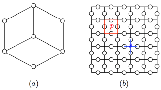
Figure 1. (a) The graph for the Steane code with three-fold cyclic symmetry. (b) The toric code on a square lattice. Qubits are sitting on edges of the lattice. $p$ denotes a plaquette, which contains $4$ qubits as shown across the red lines. $s$ denotes a star, which contains $4$ qubits as shown across the blue lines.

The toric code turns out to provide another example, as shown in Fig. 1(b), which is in some sense even worse than the Steane code example. Despite the fact that the generators of the stabilizer group for the toric code have a translational symmetry, we will show in Theorem 6.4 that one cannot find a graph with translational symmetry. However, both the Steane code and the toric code do not provide counterexamples to Theorem 4.1, as the logical zero has the desired symmetry in both cases.

Nevertheless, there might still be some interesting relationship between the permutation symmetries of $\cal{Q}$ and the symmetries of $\cal{G}$ and $\cal{C}$. Let us start with a simple case:

Corollary 6.2.

For a CWS code $\cal{Q}=(\cal{G},\cal{C})$, if both $\cal{G}$ and $\cal{C}$ have a permutation symmetry $\sigma$, then the code $\mathcal{Q}$ has the permutation symmetry $\sigma$ as well.

Proof 6.3.

This is actually a direct implication of Theorem 5.2; in this case the matrix $R$ is nothing but a permutation matrix corresponding to the permutation $\sigma$.

This turns out to be good luck, as due to the structure of the stabilizer generators of graph states, a permutation of the qubits corresponds to the same permutation of the generators $\mathchoice{\mbox{\boldmath{$\displaystyle g$}}}{\mbox{\boldmath{$\textstyle g$}}}{\mbox{\boldmath{$\scriptstyle g$}}}{\mbox{\boldmath{$\scriptscriptstyle g$}}}_{i}$, and hence also corresponds to a permutation of the coordinates in the classical code $\mathcal{C}$. Prominent examples are the $(\!(5,2,3)\!)$ code and the $(\!(5,6,2)\!)$ code, whose corresponding graph is a pentagon in both cases, and the corresponding classical codes are cyclic (see [6, Sec. IIIA,B]).

Finally, let us examine the graph symmetry for the toric code. The toric code was first proposed by Kitaev in 1997 as an example demonstrating topologically ordered quantum systems [13, 14]. The setting is a two-dimensional square lattice with periodic boundary conditions and with a qubit sitting on each edge of the lattice. There are two types of stabilizer generators:

1. (star) type, indicated in Fig. 1(b) as $s$:

   $$A_{s}^{X}=\prod_{j\in\text{star}(s)}X_{j}$$ (20)

2. (plaquette) type, indicated in Fig. 1(b) as $p$:

   $$A_{p}^{Z}=\prod_{j\in\text{plaquette}(p)}Z_{j}$$ (21)

It is straightforward to check that $A_{s}^{X}$ and $A_{p}^{Z}$ commute for any pair $s$ and $p$.

These stabilizer generators are by definition translational invariant, for the translation along each direction of the two-dimensional square lattice. What is more, one can even find an encoding graph which is also translational invariant [2]. We will show that unfortunately one cannot find a translational invariant graph to represent the toric code as a CWS code.

Theorem 6.4.

A graph corresponding to the toric code cannot have the same translational symmetry as the code.

Proof 6.5.

Let $\mathcal{T}$ be the toric code stabilizer generated by the star and plaquette operators as given by Eq. (20) and Eq. (21). Suppose that $\mathcal{Q}=(\mathcal{G},\mathcal{C})$ is a code where $\mathcal{G}$ is as symmetric as the toric code stabilizer (i. e., translational invariant) and is local Clifford equivalent to $\mathcal{T}$. This means that if we let $\mathcal{S}$ be the stabilizer of $\mathcal{Q}$, then there are local Clifford elements $C_{1},C_{2},\dots$ such that $\mathcal{S}=\widehat{C}\mathcal{T}\widehat{C}^{\dagger}$, where $\widehat{C}=C_{1}\otimes C_{2}\otimes\cdots$ (here we choose an arbitrary indexing of qubits).

Let $\sigma$ be a permutation symmetry of the toric code and define $\widehat{C}_{\sigma}=C_{\sigma(1)}\otimes C_{\sigma(2)}\otimes\cdots$. Since $\sigma$ is assumed to be a symmetry of $\mathcal{S}$ as well, we have

$$\mathcal{S}=\widehat{C}\mathcal{T}\widehat{C}^{\dagger}=\widehat{C}_{\sigma}\mathcal{T}\widehat{C}^{\dagger}_{\sigma}.$$

Then for $D_{i}=C_{i}^{\dagger}C_{\sigma(i)}$, we have $\widehat{D}\mathcal{T}\widehat{D}^{\dagger}=\mathcal{T}$, where $\widehat{D}=D_{1}\otimes D_{2}\otimes\cdots$.

Let $XXXX$ be the element of this stabilizer group $\mathcal{T}$ corresponding to some star . Since $\widehat{D}$ is local, and $XXXX$ is the only element of $\mathcal{T}$ that acts on edges corresponding to , we must have $\mathcal{D}XXXX\mathcal{D}^{\dagger}=XXXX$. The same argument applies to the $Z$-terms corresponding to a plaquette  . As a result, conjugation by $D_{i}$ maps $X$ to $\pm X$ and $Z$ to $\pm Z$. Hence $D_{i}$ is an element of the Pauli group.

Now we know that $\widehat{D}$ is in the Pauli group, and it holds for every permutation $\sigma$. On the other hand, the symmetry group of the toric code is transitive. Therefore, for every $i$, $j$, the product $C_{i}^{\dagger}C_{j}$ is in the Pauli group, and furthermore

$$C_{1}\otimes C_{2}\otimes\cdots=(H\otimes H\otimes\cdots)(P_{1}\otimes P_{2}\otimes\cdots),$$

where the factors $P_{i}$ are in the Pauli group and $H$ is some Clifford element acting on a single qubit.

$\widehat{C}\mathcal{T}\widehat{C}^{\dagger}$ is supposed to correspond to a graph state, but $(P_{1}\otimes P_{2}\otimes\cdots)$ just changes some signs in the stabilizer group, and $(H\otimes H\otimes\cdots)$ cannot turn the stabilizer group of the toric code into a graph-type stabilizer group.

7. Summary and Discussion

In this work we have investigated the symmetry properties of CWS codes. Our main result shows that for a given CWS code $\mathcal{Q}$ with some permutation symmetry $\sigma$, there always exits a stabilizer state $\mathcal{S}$ with the same symmetry $\sigma$ such that $\mathcal{Q}=(\mathcal{S},\mathcal{C})$ for some classical code $\mathcal{C}$. As many good CWS codes are found by starting from a chosen $\mathcal{S}$, this ensures that when trying to find CWS codes with certain permutation symmetry, the choice of $\mathcal{S}$ with the same symmetry will suffice. A key point to reach our main result is to obtain a canonical representation for CWS codes, i. e., a unique decomposition as USt codes.

One natural question is whether there is any chance to find a classical code $\mathcal{C}$ with the same symmetry $\sigma$ as that of $\mathcal{Q}$, which, together with some $\mathcal{S}$ with symmetry $\sigma$, gives $\mathcal{Q}=(\mathcal{S},\mathcal{C})$. We do not know the answer in general, but we know that one can no longer restrict $\mathcal{S}$ to the stabilizer used in the canonical form, but might have to introduce some phase factors. We have developed a sufficient condition that $\mathcal{C}$ has to satisfy in order to ensure that in combination with some $\mathcal{S}$ with symmetry $\sigma$, one will have $\mathcal{Q}=(\mathcal{S},\mathcal{C})$ with the same symmetry $\sigma$. Observing the fact that the permutation on the code $\mathcal{Q}$ does not directly translate into a permutation of the classical $\mathcal{C}$ (but a linear transformation given by the matrix $R$), in general one cannot expect to find a classical code $\mathcal{C}$ with the same symmetry as that of $\mathcal{Q}$.

One interesting case are cyclic codes. If there exists a graph $\mathcal{G}$ which has the same symmetry $\sigma$ as the CWS code $\mathcal{Q}=(\mathcal{G},\mathcal{C})$, then the permutation of the code $\mathcal{Q}$ translates directly into a permutation of the classical code $\mathcal{C}$. Hence, combining a graph $\mathcal{G}$ whose symmetry group contains the cyclic group of order $n$, with a cyclic classical code $\mathcal{C}$ of length $n$, gives a cyclic CWS code $\mathcal{Q}=(\mathcal{G},\mathcal{C})$. It would be nice to see whether the converse is true as well, i. e., given a cyclic CWS code $\mathcal{Q}$ which corresponds to a graph $\mathcal{G}$ whose symmetry group contains the cyclic group of order $n$, can we always find a cyclic classical code $\mathcal{C}$ of length $n$, such that $\mathcal{Q}=(\mathcal{G},\mathcal{C})$. We leave this for future investigation.

In general, although every CWS code $\mathcal{Q}$ is local Clifford equivalent to a standard form $(\mathcal{G},\mathcal{C})$, the local Clifford operation may destroy the permutation symmetry of the original code. In other words, one cannot expect to always find a graph $\mathcal{G}$ which has the same symmetry as that of $\mathcal{Q}$. The seven-qubit Steane code is such an example where the graph can only possess a three-fold cyclic symmetry which is the symmetry of the stabilizer generators, instead of the seven-fold cyclic symmetry of the code. For the toric code, despite the stabilizer generators being translational invariant, we show that there does not exist any associated translational invariant graph. A general understanding of the conditions that graphs can possess the same symmetry as the CWS code is worth further investigation.

Acknowledgements

SB was in part supported by National Elites Foundation and by a grant from IPM (No. 91810409). JC is supported by NSERC and NSF of China (Grant No. 61179030). The CQT is funded by the Singapore MoE and the NRF as part of the Research Centres of Excellence programme. ZJ acknowledges support from NSERC, ARO and NSF of China (Grant Nos. 60736011 and 60721061). QW is supported by NSERC. BZ is supported by NSERC and CIFAR. MG acknowledges support by the Intelligence Advanced Research Projects Activity (IARPA) via Department of Interior National Business Center contract No. D11PC20166. The U.S. Government is authorized to reproduce and distribute reprints for Governmental purposes notwithstanding any copyright annotation thereon. Disclaimer: The views and conclusions contained herein are those of the authors and should not be interpreted as necessarily representing the official policies or endorsements, either expressed or implied, of IARPA, DoI/NBC, or the U.S. Government.

The authors would like to thank Martin Rötteler for his suggestion to use the Fourier transformation to prove Lemma 3.6.

References

• [1] S.ย Beigi, I.ย Chuang, M.ย Grassl, P.ย Shor, and B.ย Zeng. Graph concatenation for quantum codes. Journal of Mathematical Physics, 52(2):022201, February 2011.
• [2] S.ย Bravyi and R.ย Raussendorf. Measurement-based quantum computation with the toric code states. Physical Review A, 76(2):022304, August 2007.
• [3] A.ย R. Calderbank, E.ย Rains, P.ย W. Shor, and N.ย J.ย A. Sloane. Quantum error correction via codes over ${GF}(4)$. IEEE Transactions on Information Theory, 44(4):1369โ€“1387, 1998.
• [4] A.ย R. Calderbank and P.ย W. Shor. Good quantum error-correcting codes exist. Physcial Review A, 54:1098โ€“1105, August 1996.
• [5] I.ย Chuang, A.ย Cross, G.ย Smith, J.ย Smolin, and B.ย Zeng. Codeword stabilized quantum codes: Algorithm and structure. Journal of Mathematical Physics, 50(4):042109, April 2009.
• [6] A.ย Cross, G.ย Smith, J.ย A. Smolin, and B.ย Zeng. Codeword stabilized quantum codes. IEEE Transactions on Information Theory, 55(1):433โ€“438, 2009.
• [7] L.ย E. Danielsen. On self-dual quantum codes, graphs, and Boolean functions. Masterโ€™s thesis, University of Bergen, 2005. http://arxiv.org/abs/quant-ph/0503236.
• [8] S.ย Dutta and P.ย P Kurur. Quantum Cyclic Code. Preprint arXiv:1007.1697 [cs.IT], June 2010.
• [9] D.ย Gottesman. Stabilizer Codes and Quantum Error Correction. PhD thesis, California Institute of Technology, Pasadena, CA, 1997.
• [10] M.ย Grassl, A.ย Klappenecker, and M.ย Rรถtteler. Graphs, quadratic forms, and quantum codes. In Proceedings 2002 IEEE International Symposium on Information Theory (ISIT 2002), pageย 45, Lausanne, Switzerland, June/July 2002. http://arxiv.org/abs/quant-ph/0703112.
• [11] M.ย Grassl and M.ย Rรถtteler. Non-additive quantum codes from Goethals and Preparata codes. Proceedings of 2008 IEEE Information Theory Workshop, pages 396โ€“400, 2008.
• [12] M.ย Grassl and M.ย Rรถtteler. Quantum Goethals-Preparata codes. Proceedings of 2008 IEEE International Symposium on Information Theory, pages 300โ€“304, 2008.
• [13] A.ย Yu. Kitaev. Quantum computations: algorithms and error correction. Russian Math. Surveys, 52:1191โ€“1249, 1997.
• [14] A.ย Yu. Kitaev, A.ย H. Shen, and M.ย N. Vyalyi. Classical and Quantum Computation, volumeย 47 of Graduate Studies in Mathematics. American Mathematical Society, Providence, RI, 2002.
• [15] E.ย Knill. Group Representations, Error Bases and Quantum Codes. Technical Report LAUR-96-2807, LANL, 1996. Preprint http://arxiv.org/quant-ph/9608049.
• [16] E.ย Knill. Non-binary Unitary Error Bases and Quantum Codes. Technical Report LAUR-96-2717, LANL, 1996. Preprint http://arxiv.org/quant-ph/9608048.
• [17] Y.ย Li, I.ย Dumer, and L.ย P. Pryadko. Clustered Error Correction of Codeword-Stabilized Quantum Codes. Physical Review Letters, 104(19):190501, May 2010.
• [18] S.ย Y. Looi, L.ย Yu, V.ย Gheorghiu, and R.ย B. Griffiths. Quantum error correcting codes using qudit graph states. Physical Review A, 78(4):042303, 2008.
• [19] F.ย J. MacWilliams and N.ย J.ย A. Sloane. The Theory of Error-Correcting Codes. North-Holland Publishing Company, Amsterdam, 1977.
• [20] M.ย Nielsen and I.ย Chuang. Quantum computation and quantum information. Cambridge University Press, Cambridge, England, 2000.
• [21] C.ย E. Shannon. A mathematical theory of communication. Bell Labs Technical Journal, 27:379โ€“423, 1948.
• [22] A.ย Steane. Multiple particle interference and quantum error correction. Proceedings of the Royal Society of London, Series A, 452:2551โ€“2577, 1996.
• [23] S.ย Yu, Q.ย Chen, and C.ย H. Oh. Graphical quantum error-correcting codes. Preprint arXiv:0709.1780 [quant-ph], September 2007.