Application of the G-JF Discrete-Time Thermostat for Fast and Accurate Molecular Simulations

Abstract

A new Langevin-Verlet thermostat that preserves the fluctuation-dissipation relationship for discrete time steps, is applied to molecular modeling and tested against several popular suites (AMBER, GROMACS, LAMMPS) using a small molecule as an example that can be easily simulated by all three packages. Contrary to existing methods, the new thermostat exhibits no detectable changes in the sampling statistics as the time step is varied in the entire numerical stability range. The simple form of the method, which we express in the three common forms (Velocity-Explicit, Störmer-Verlet, and Leap-Frog), allows for easy implementation within existing molecular simulation packages to achieve faster and more accurate results with no cost in either computing time or programming complexity.

I Introduction

Recently, a new stochastic thermostat G-JF , based on an exact implementation of the fluctuation-dissipation relationship in discrete time, was presented as integrated into the well-known and widely used Verlet formalism. It was analytically demonstrated that the method provides exact thermodynamic response for both flat and harmonic potentials for any time step within the Verlet stability criteria. This unique thermodynamic feature of the approach, as implemented into the Verlet framework, makes it attractive for a wide range of applications, where it is desired to execute efficient and accurate simulations. Here, we demonstrate that the G-JF method of Ref. G-JF is not limited to simple linear cases, but also extends its usefulness to complex nonlinear systems.

Langevin dynamic simulations constitute an appealing approach for simulations of physical systems in contact with a thermodynamic heat bath. A very popular class of such systems is molecular dynamics (MD) Frenkel_1996 of classical particle ensembles. The method is based on numerical integration of the Langevin equation

$$m\dot{v} = f(r,t)-\alpha\dot{r}+\beta(t)\,,$$ (1)

where $r$ is the coordinate, $v=\dot{r}$ is its velocity, $m$ is its mass, $f$ is a net deterministic force acting on $r$. The friction constant $\alpha>0$ and the noise $\beta$ are connected by the fluctuation-dissipation relationship Parisi_1988

$$\langle\beta(t)\rangle = 0$$ (2)

$$\langle\beta(t)\beta(t^{\prime})\rangle = 2\alpha k_{B}T\delta(t-t^{\prime})$$ (3)

with $k_{B}$ and $T$ being Boltzmann’s constant and the thermodynamic temperature, respectively. Given the applicability of this equation to a wide spectrum of physical systems with phenomenological dissipation and thermal noise, there have been decades of development in numerical methods for solving such equations. Specifically, the perfection of the most important thermodynamic properties of discrete-time numerical simulations have been of particular interest. We here point to the vast literature through Refs. G-JF ; LM ; Brunger_1984 ; Loncharich_2004 ; vdSpoel_2005 ; Goga_2012 ; Schneider_1978 ; vGunsteren_1988 ; V-EC and references therein. The most commonly sought after properties in stochastic simulations have been i) diffusion of a particle in a flat potential, ii) transport on a linear ramp potential (which can be mapped directly onto the diffusive behavior in a flat potential), and iii) Boltzmann sampling in harmonic potentials notice_on_methods . Since the G-JF method G-JF exhibits all these features thermodynamically correct in discrete time, we here wish to provide additional expressions for practical implementation of the method. We also provide a simple, yet representative, example of how the method performs for a nonlinear and complex system in comparison to several widely used contemporary molecular dynamics simulation suites.

II The Three Verlet Expressions

Verlet integrators are usually expressed in one of three forms Allen : A) velocity-explicit Verlet (VE), which advances the trajectory one time step based on the coordinate and its conjugate variable (here the velocity), B) Störmer-Verlet (SV), which uses coordinates at two consecutive time steps to advance time, and C) leap-frog (LF), which advances the trajectory based on the coordinate and its conjugate variable, the latter being represented at half-integer time steps relative to the coordinate. The three typical Verlet formulations produce identical trajectories, and, thus, are different expressions of the exact same method. Consequently, applications of the Verlet method are commonly expressed in any of the available forms. Since all three identical methods are frequently used in the literature, we start here with the recently published G-JF thermostat that was derived in the natural VE form, and re-express the algorithm in the two other popular forms. The previous harmonic oscillator analysis G-JF of the method applies to all three variants since they produce identical results. Specifically, the three following formulations will result in the correct fluctuation-dissipation relationship and thus, the correct thermodynamic response in linear systems.

II.1 Velocity Explicit G-JF

We take our starting point with the VE G-JF expressions that were derived and analyzed in G-JF . Denoting discrete time variables by the integer time step superscript, such that, e.g., $r^{n}=r(t_{n})$, the algorithm for advancing $r^{n}$ and $v^{n}$ one time step of $dt$ reads

$$r^{n+1} = r^{n}+b\,dt\,v^{n}+\frac{b\,dt^{2}}{2m}f^{n}+\frac{b\,dt}{2m}\beta^{n+1}$$ (4)

$$v^{n+1} = av^{n}+\frac{dt}{2m}(af^{n}+f^{n+1})+\frac{b}{m}\beta^{n+1}\,,$$ (5)

where

$$a = \frac{1-\frac{\alpha dt}{2m}}{1+\frac{\alpha dt}{2m}}\;\;,\;\;b\;=\;\frac{1}{1+\frac{\alpha dt}{2m}}\,,$$ (6)

and where

$$\beta^{n+1} = \int_{t_{n}}^{t_{n+1}}\beta(t^{\prime})\,dt^{\prime}$$ (7)

is a standard Gaussian random number that satisfies

$$\langle\beta^{n}\rangle = 0\;\;,\;\;\langle\beta^{n}\beta^{l}\rangle\;=\;2\alpha k_{B}Tdt\delta_{n,l}\,.$$ (8)

Setting the initial conditions $(r^{0},v^{0})$, Eqs. (4)-(8) can be directly used to generate the trajectory $(r^{n},v^{n})$ from which the dynamical and statistical information can be derived.

II.2 Störmer-Verlet G-JF

We here start by rewriting Eqs. (4) and (5) for $n\rightarrow n-1$:

$$r^{n} = r^{n-1}+b\,dt\,v^{n-1}+\frac{b\,dt^{2}}{2m}f^{n-1}+\frac{b\,dt}{2m}\beta^{n}$$ (9)

$$v^{n} = av^{n-1}+\frac{dt}{2m}(af^{n-1}+f^{n})+\frac{b}{m}\beta^{n}\,.$$ (10)

As outlined in Ref. G-JF , Eq. (10) can be inserted into Eq. (4) in order to replace $v^{n}$, whereafter Eq. (9) is used to replace the resulting $v^{n-1}$. This yields

$$r^{n+1} = 2br^{n}-ar^{n-1}+\frac{b\,dt^{2}}{m}f^{n}+\frac{b\;dt}{2m}(\beta^{n}+\beta^{n+1})\,,$$

which is the SV formulation of the G-JF method. Unlike the VE expressions, the SV equation does not contain direct information about the velocity and is therefore not directly applicable for natural initial conditions $(r^{0},v^{0})$. The self-consistent approach for starting this procedure from $(r^{0},v^{0})$ is to apply Eq. (9) for $n=0$,

$$r^{1} = r^{0}+b\,dt\,v^{0}+\frac{b\,dt^{2}}{2m}f^{0}+\frac{b\,dt}{2m}\beta^{1}\,,$$ (12)

then apply Eq. (LABEL:eq:Eq_SV_1a) for all subsequent time steps $n>0$. In order to calculate both the complete dynamical trajectory and important thermodynamic quantities, one needs the velocity $v^{n}$ explicitly expressed as well. Consistent with the method, we replace $v^{n-1}$ in Eq. (10) by inserting Eq. (9), such that

$$v^{n} = \frac{a}{b}\frac{r^{n}-r^{n-1}}{dt}+\frac{dt}{2m}f^{n}+\frac{1}{2m}\beta^{n}$$

$$= \frac{r^{n+1}-(b-a)r^{n}-ar^{n-1}}{2dtb}+\frac{1}{4m}(\beta^{n}-\beta^{n+1})\,.$$

Thus, Eqs. (LABEL:eq:Eq_SV_1a), (12), and (LABEL:eq:Eq_SV_5a) constitute the identical SV form of the VE expressions.

II.3 Leap-Frog G-JF

This version of the Verlet method for Langevin equations comes with some flexibility in how the method is expressed. We take the starting point with the SV form given in Eq. (LABEL:eq:Eq_SV_1a) and introduce a reasonable definition of the half-step velocity

$$v^{n+\frac{1}{2}} = \frac{r^{n+1}-r^{n}}{dt}\,.$$ (14)

We now use Eq. (14) to replace $r^{n+1}$ in Eq. (LABEL:eq:Eq_SV_1a) to obtain

$$v^{n+\frac{1}{2}} = a\frac{r^{n}-r^{n-1}}{dt}+\frac{b\,dt}{m}f^{n}+\frac{b}{2m}(\beta^{n}+\beta^{n+1})\,,$$

in which we can again apply Eq. (14) and arrive at

$$v^{n+\frac{1}{2}} = av^{n-\frac{1}{2}}+\frac{b\,dt}{m}f^{n}+\frac{b}{2m}(\beta^{n}+\beta^{n+1})\,.$$ (16)

This equation is the half-time step velocity propagator, which is complemented by Eq. (14) to yield a LF G-JF method

$$r^{n+1} = r^{n}+dt\,v^{n+\frac{1}{2}}\,.$$ (17)

As was the case for the SV formulation of the method, this LF representation does not trivially incorporate the natural initial conditions $(r^{0},v^{0})$. We therefore apply Eq. (14) for $n=0$ in combination with Eq. (12), resulting in

$$v^{\frac{1}{2}} = bv^{0}+\frac{b\,dt}{2m}f^{0}+\frac{b}{2m}\beta^{1}\,,$$ (18)

to be used, along with Eq. (12), before applying Eqs. (16) and (17) for $n>0$. The proper integer-step velocity can be found from combining Eqs. (16) and (4), resulting in

$$v^{n+\frac{1}{2}} = av^{n-\frac{1}{2}}+2\frac{r^{n+1}-r^{n}}{dt}-2bv^{n}+\frac{b}{2m}(\beta^{n+1}-\beta^{n})\,,$$

where we can then, again, use Eq. (14) to obtain

$$v^{n} = \frac{1}{2b}(v^{n+\frac{1}{2}}+av^{n-\frac{1}{2}})+\frac{1}{4m}(\beta^{n}-\beta^{n+1})\,.$$ (20)

Thus, Eqs. (16), (17), and (20) constitute a consistent LF method, where initial conditions $(r^{0},v^{0})$ are applied through Eqs. (12) and (18).

Notice that while the given SV method is uniquely connected to the VE expressions in both the coordinate $\{r^{n}\}$ and its evaluated velocity $\{v^{n}\}$, the development of LF is not unique, even if LF is constructed to produce identical trajectories $(r^{n},v^{n})$ to those of VE and SV. The reason is the aforementioned somewhat ambiguous choice in defining the half-step velocity $v^{n+\frac{1}{2}}$ in Eq. (14), and the subsequent reconstruction of the integer-time velocity $v^{n}$ in Eq. (20). Thus, one can exercise some freedom of choice in the velocity equations when using the LF expressions.

For example, a sensible alternative to the half-step velocity in Eq. (14) may be

$$u^{n+\frac{1}{2}} = \frac{r^{n+1}-r^{n}}{bdt}-\frac{1}{2m}\beta^{n+1}\,,$$ (21)

where we use the symbol $u$ for the revised definition of the half-step velocity. Following the procedure starting from Eq. (14), we can develop the following alternate LF formulation, which also yields identical trajectories $(r^{n},v^{n})$. The two equations for half-step velocity and integer-step position become

$$u^{n+\frac{1}{2}} = au^{n-\frac{1}{2}}+\frac{dt}{m}f^{n}+\frac{1}{2m}\beta^{n}\,.$$ (22)

$$r^{n+1} = r^{n}+b\,dt\,u^{n+\frac{1}{2}}+\frac{b\,dt}{2m}\beta^{n+1}\,,$$ (23)

with initiating half-step velocity $u^{\frac{1}{2}}$ and conversion to integer-step velocity $v^{n}$ written

$$u^{\frac{1}{2}} = v^{0}+\frac{dt}{2m}f^{0}$$ (24)

$$v^{n} = \frac{1}{2}(u^{n+\frac{1}{2}}+au^{n-\frac{1}{2}})+\frac{1}{4m}\beta^{n}\,,$$ (25)

respectively. As mentioned above, all LF formulations of the thermostat yield identical trajectories for $(r^{n},v^{n})$ and therefore constitute the same method regardless of the specific definition of the half-step velocity. Choosing which one to use is entirely a matter of convenience. The defined half-step velocity is simply an auxiliary variable, which need not have any specific useful physical interpretation for the evaluation of thermodynamic quantities.

III Testing the method

We exemplify the applicability of the G-JF method in the context of a simple biomolecular simulation and we make comparison to results of the widely-used molecular dynamics codes AMBER Cornell_1995 , LAMMPS LAMMPS-Manual ; Plimpton_1995 , and GROMACS vdSpoel_2005 . These packages employ different commonly used stochastic thermostats. More comprehensive discussions of other thermostats can be found in recent references G-JF ; LM ; Goga_2012 . The purpose of the following simulations is not to present new or ground-breaking results in biomolecular science; instead, we choose a simple and well-understood representative model system that can illuminate, through simulations within well-established MD packages, some key features of the new algorithm as implemented into one of the codes that is particularly amenable to revisions.

III.1 Simulation Details

We performed classical molecular dynamics simulations of alanine dipeptide (illustrated in Figure 1a), a small and well-studied biomolecule. Intramolecular interactions among the solute atoms, including bond, angle, dihedral, and non-bonded energies, were modeled with an AMBER classical all-atom molecular mechanical treatment Cornell_1995 , coupled with the recent ff12 parameter set Case_2012 , while the extra-molecular environment was treated as vacuum.

This model system was simulated at a target temperature of 300 K with four integration schemes for comparison: i) The BBK thermostat Brunger_1984 , which is implemented and expressed within AMBER 12 (ntt=3) in the leap-frog Verlet formulation Loncharich_2004 ; ii) the method of Schneider & Stoll Schneider_1978 , as implemented in the LAMMPS simulation software LAMMPS-Manual (with the combination of the nve and langevin fixes); iii) a variation of the method of van Gunsteren & Berendsen vGunsteren_1982 ; vGunsteren_1988 , implemented in GROMACS vdSpoel_2005 (as the sd integrator Scott_1999 ), which includes velocity rescaling; and finally iv) the G-JF thermostat G-JF .

The latter was implemented into AMBER through small modifications to the AMBER 12 source code Case_2012 . Since the underlying LF Verlet integrator used in the BBK method is consistent with Eqs. (16), (17), and (20), revisions were only necessary with regard to the fluctuation terms. The memory framework was modified to include space for the correlating noise term from the previous time step, corresponding to $\beta^{n}$ in Eqs. (16) and (20), to be cached for use in subsequent integration steps. A Langevin damping coefficient of 10 ps^-1 was used throughout all the simulations. Simulation input data for LAMMPS and GROMACS runs were generated directly from AMBER-formatted coordinate and topology files using the free tools amber2lammps.py (distributed with the LAMMPS source code), and amb2gmx.pl amb2gmx , respectively.

Data were collected from sets of ten independent 100 ps simulations at several values of the integration time step, from 0.5–3.1 fs in increments of 0.1 fs, and from 3.1–3.2 fs in increments of 0.01 fs. Each simulation was initiated from the same energy-minimized starting structure of the peptide. For each independent simulation, initial atomic velocities were assigned from a Maxwell-Boltzmann distribution appropriate to the target temperature and the psuedo-random number chain was uniquely seeded.

First and second moments of the total potential energy distribution were chosen as measures of the stability and accuracy with which each integration method could reproduce the statistical-mechanical properties of the physical system. Average energy and its fluctuation were computed based on samples at all integration steps. The total number of integration steps $N$ was varied based on the time step $dt$, such that $N=\lfloor 100~{}\mathrm{ps}/dt\rfloor$.

III.2 Results

Figures 1b and c summarize the results and shows the average total potential energy and its standard deviation as a function of the simulated time step for all the integration methods. As expected, all methods give very similar results for both the average and standard deviation of the energies for as long as the time steps are smaller than about 1 fs.

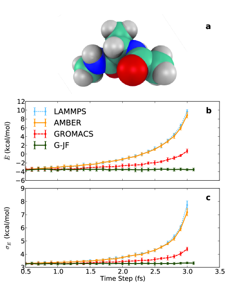
Figure 1: (a) Space-filling model of the simulated alanine dipeptide (Ac-Ala-NHMe) molecule. (b) Mean and (c) standard deviation of the potential energy in the model alanine dipeptide, computed with different molecular dynamics codes and various time steps. Results are depicted as follows, top curve to bottom: Blue for LAMMPS; orange for AMBER; red for GROMACS; and green for AMBER with the G-JF implementation.

However, for increasing time steps the unmodified contemporary codes start deviating from the expected statistical values found for small $dt$. The two strongest deviations are found for the BBK method, implemented in AMBER 12, and the thermostat of Schneider & Stoll, implemented into LAMMPS. The same deviating behavior, albeit seemingly with only one third deviation, is found for the thermostat of van Gunsteren & Berendsen, implemented into GROMACS. In contrast, the G-JF method, implemented into AMBER 12 as described above, shows the inherent feature of preserving the fluctuation-dissipation relationship for any time step. In fact, for these simulations, the G-JF method can give statistical estimates at all time steps up to the stability limit that are indistinguishable from those at small time steps. The stability limit is here identified by adiabatically increasing the time step of a simulation until simulations produce anomalously high velocities, indicating that the Verlet integrator is no longer capable of producing a meaningful trajectory for the simulation. The existing stochastic thermostats seem stable up to 3.0 fs for this simulation, while the G-JF is stable for up to a slightly higher value 3.1 fs.

We close this section by arguing for the use of potential energy (and its fluctuations) as a measure for the ability of the different thermostats to correctly sample the phase space corresponding to the target temperature. A seemingly more straightforward test would be to consider the kinetic energy. However, as shown in Ref. G-JF for the harmonic oscillator case, the computed velocity $v^{n}$, and thereby the kinetic energy, is increasingly depressed for increasing time step in any Verlet scheme, regardless of the inclusion of a thermostat. Thus, when evaluating a thermostat, measures of velocity and kinetic energy may not be appropriate for determining the quality of statistical sampling. Further, this observation may hint at statistical sampling problems arising from thermostats that involve “velocity rescaling” as a way to obtain a desired temperature.

IV Discussion and Conclusion

The newly developed G-JF stochastic Verlet thermostat has been applied to simulations of a small, yet non-trivial and nonlinear, system representative of many applications in molecular modeling. It has previously been analytically demonstrated that for linear systems the new method yields exact statistical behavior of diffusion and Boltzmann distributions for any time step leading to stable dynamics G-JF . The simulations presented here indicate that these attractive and robust statistical features are likely to remain in other complex and nonlinear systems. Specifically, our present simulations demonstrate that the statistical behavior of potential energy remains sound for any time step up to the limit where the atomic trajectories suddenly diverge. In contrast, available contemporary molecular dynamics codes with other stochastic thermostats show deviating behavior for increasing time step, indicating that the interpretation of thermodynamic data from those algorithms must be done with caution and small time steps. This seems to be the case for the three popular molecular dynamics codes that we have investigated here, and is likely to be true also for other available MD simulation codes. In order to facilitate comparison between the stochastic thermostats, we use the same AMBER force fields in all four sets of simulations. We emphasize that simulations with the G-JF thermostat have been completed by implementing the new simple algorithm into an existing available code (AMBER 12), to ensure direct comparison between the thermostats without any other differences in parameters or simulation details. Thus, based on the preliminary tests and analyses, we suggest that the algorithm presented here and in Ref. G-JF be implemented into existing molecular dynamics codes for further use and evaluation. In order to facilitate such revisions, we have explicitly provided the algorithm in all three commonly used formulations of the Verlet method.

- (1) N. Grønbech-Jensen and O. Farago, Mol. Phys. 111, 983 (2013).
- (2) See, e.g., D. Frenkel and B. Smit, Understanding Molecular Simulation, From Algorithm to Application, (Academic Press, 1996).
- (3) See, e.g., G. Parisi, Statistical Field Theory, (Addison Wesley, Menlo Park, 1988).
- (4) B. Leimkuhler and C. Matthews, Appl. Math. Res. eXpress, 2013, 34 (2012).
- (5) N. Goga, A.J. Rzepiela, A.H. de Vries, S.J. Marrink, H.J.C. Berendsen, J. Chem. Th. Comp. (2012) DOI: 10.1021/ct3000876.
- (6) E. Vanden-Eijnden and G. Ciccotti, Chem. Phys. Lett. 429, 310 (2006).
- (7) D. van der Spoel, E. Lindahl, B. Hess, G. Groenhof, A. E. Mark, and H. J. C. Berendsen, J. Comp. Chem. 26, 1701 (2005).
- (8) R. J. Loncharich, B. R. Brooks, and R. W. Pastor, Biopolymers 32, 523 (2004).
- (9) W. F. van Gunsteren, H. J. C. Berendsen, Mol Simul. 1, 173 (1988).
- (10) A. Brünger, C. L. Brooks, and M. Karplus, Chem. Phys. Lett. 105, 495 (1984).
- (11) T. Schneider and E. Stoll, Phys. Rev. B 17, 1302 (1978).
- (12) We notice that most recent methods are capable of reproducing correct statistical properties for diffusion in a flat potential and approximate results for the harmonic oscillator. In contrast, the method given in LM gives good statistical results for the harmonic oscillator, but does not correctly reproduce spatial diffusion (as calculated from the Einstein relation) in a flat potential.
- (13) See, e.g., M. P. Allen and D. J. Tildesley, Computer Simulation of Liquids, (Oxford University Press, Inc., New York, 1989).
- (14) W. D. Cornell, P. Cieplak, C. I. Bayly, I. R. Gould, K. M. Merz, D. M. Ferguson, D. C. Spellmeyer, T. Fox, J. W. Caldwell, and P. A. Kollman, J. Am. Chem. Soc. 117, 5179 (1995).
- (15) D. A. Case, T. A. Darden, T. E. Cheatham, III, C. L. Simmerling, J. Wang, R. E. Duke, R. Luo, R. C. Walker, W. Zhang, K. M. Merz, B. Roberts, S. Hayik, A. Roitberg, G. Seabra, J. Swails, A. W. Goetz, I. Kolossv ry, K. F. Wong, F. Paesani, J. Vanicek, R. M. Wolf, J. Liu, X. Wu, S. R. Brozell, T. Steinbrecher, H. Gohlke, Q. Cai, X. Ye, J. Wang, M.-J. Hsieh, G. Cui, D. R. Roe, D. H. Mathews, M. G. Seetin, R. Salomon-Ferrer, C. Sagui, V. Babin, T. Luchko, S. Gusarov, A. Kovalenko, and P. A. Kollman (2012), AMBER 12, University of California, San Francisco.
- (16) See http://lammps.sandia.gov/doc/Manual.pdf (Jan. 24, 2013), section 6.16, for the description of the “fix_langevin” command.
- (17) S. J. Plimpton, J. Comp. Phys. 117, 1 (1995).
- (18) W. F. van Gunsteren, H. J. C. Berendsen, Mol. Phys. 45, 637 (1982).
- (19) W. R. P. Scott, P. H. Hünenberger, I. G. Tironi, A. E. Mark, S. R. Billeter, J. Fennen, A. E. Torda, T. Huber, P. Krüger, and W. F. van Gunsteren, J. Phys. Chem. A 103, 3596 (1999).
- (20) D. L. Mobley, J. D. Chodera, and K. A. Dill, J. Chem. Phys. 125, 084902, (2006).