Analysis of Spin-Orbit Misalignment in Eclipsing Binary DI Herculis

Abstract

Eclipsing binary DI Herculis (DI Her) is known to exhibit anomalously slow apsidal precession, below the rate predicted by the general relativity. Recent measurements of the Rossiter-McLauglin effect indicate that stellar spins in DI Her are almost orthogonal to the orbital angular momentum, which explains the anomalous precession in agreement with the earlier theoretical suggestion by Shakura. However, these measurements yield only the projections of the spin-orbit angles onto the sky plane, leaving the spin projection onto our line of sight unconstrained. Here we describe a method of determining the full three-dimensional spin orientation of the binary components relying on the use of the gravity darkening effect, which is significant for the rapidly rotating stars in DI Her. Gravity darkening gives rise to nonuniform brightness distribution over the stellar surface, the pattern of which depends on the stellar spin orientation. Using archival photometric data obtained during multiple eclipses spread over several decades we are able to constrain the unknown spin angles in DI Her with this method, finding that spin axes of both stars lie close to the plane of the sky. Our procedure fully accounts for the precession of stellar spins over the long time span of observations.

1. Introduction.

The binary system DI Herculis (DI Her, HD 175227) was discovered as an eclipsing variable by Hoffmeister (1930). It consists of two massive B stars on an eccentric orbit ($e=0.49$) with period $P=10^{d}.55$, inclined at an angle $i=89.3^{\circ}$ with respect to our line of sight (see Table 1 for parameters of both binary components). A unique property of this system that has been attracting a lot of attention for almost three decades is its low rate of apsidal precession, $\dot{\omega}_{obs}=1.24^{\circ}\pm 0.18^{\circ}/100$ yr (Martynov & Khaliullin 1980). This is almost two times lower than the general relativistic apsidal precession rate $\dot{\omega}_{\rm GR}=2.35^{\circ}/100$ yr theoretically predicted based on the measured parameters of the system (Rudkjobing 1959). For a long time this discrepancy was not understood (Maloney et al. 1989) and even ascribed to the failure of general relativity (Moffat 1989).

Shakura (1985) suggested that slow apsidal precession in DI Her is caused by the misalignment between the spin and orbital angular momentum axes of the system. Indeed, for stellar spins strongly misaligned with the orbital angular momentum the rotation-induced stellar quadrupole gives rise to a contribution to $\dot{\omega}$ with a sign opposite to that of $\dot{\omega}_{\rm GR}$. Then, if this quadrupole-induced precession is fast enough it can easily alter the full rate of apsidal precession and even make it smaller than $\dot{\omega}_{\rm GR}$ as in the case of DI Her. Somewhat less extreme version of this idea has recently been applied to another eclipsing binary AS Camelopardalis (Pavlovski et al. 2011), which also exhibits relatively slow rate of apsidal precession.

The spin-orbit misalignment in DI Her has been recently confirmed by Albrecht et al. (2009) who used the evolution of stellar spectral signatures during the eclipse (the so-called Rossiter-McLaughlin effect, Holt 1893; Rossiter 1924; McLaughlin 1924) to set constraints on the spin orientation of both stars. They found that both stars of DI Her have their spin axes nearly perpendicular to the orbital angular momentum axis, which is at odds with the common wisdom regarding spin-orbit orientation in close binary stars, but can naturally explain the slow apsidal precession in this system.

Unfortunately, the Rossiter-McLaughlin effect allows one to determine only the sky plane projection $\lambda$ of the angle $\alpha$ between the spin and orbital momentum axes for the stars. The angle $\beta$ between the stellar spin and our line of sight remains essentially unconstrained. However, figuring out whether spin-orbit misalignment can explain the observed $\dot{\omega}$ does depend on the value of $\beta$, since the stellar spin frequency $\omega$ is inferred from the measured projected stellar rotation speed $v_{rot}\sin\beta=\omega R_{\star}\sin\beta$ ($R_{\star}$ is the stellar radius). Albrecht et al. (2009) and Claret et al. (2010) tackled the issue of undetermined $\beta$ by means of Monte Carlo simulations, assuming this angle to be uniformly distributed.

In this work we develop a method of analyzing the photometric eclipse data, which allows us to constrain the angle $\beta$ without using spectroscopic data. This method relies on the fact that both components of DI Her are rapidly rotating stars ($v_{rot}\sin\beta$ exceeds $100$ km s^-1 for both components, see Table 1), and must exhibit a non-uniform surface brightness distribution due to the gravity darkening effect (von Zeipel 1924). This surface brightness pattern is sensitive to the orientation of stellar spin axis with respect to our line of sight. By probing the brightness distribution via the detailed shape of the system lightcurve during the eclipse one can infer the full spin orientation of both stars. Analogous method was recently proposed by Barnes (2009) for analyzing planetary transits around rapidly rotating stars, and applied by Szabó et al. (2011) and Barnes et al. (2011) to determine the spin-orbit misalignment in a transiting system KOI-13.01.

In determining the unknown angles $\beta$ for both stellar components we also use other constraints on the system parameters, such as the observed apsidal precession rate and the evolution of the projected stellar rotation velocities $v_{rot}\sin\beta$ over the long time span.

This work is organized as follows. In §2 we describe geometric setup of the problem, and eclipse lightcurve modeling. In §3 we describe observational data and our fitting procedure. Our results are presented in §4 and discussed in §5. In Appendix B we derive equations describing evolution of the system orientation as a result of spin and orbital precession, which may find other applications.

2. Eclipse modeling.

2.1. Geometry of the system.

To model eclipse lightcurve we use two Cartesian coordinate systems. One is the observer frame $(X,Y,Z)$, which describes the orbital orientation of the system: $Z$ axis points from the system barycenter towards the observer, $X$ axis is along the direction of the sky-projected orbital angular momentum and $Y$ axis is aligned with the line of nodes, see Figure 1.

Another system $(x_{i},y_{i},z_{i})$, where $i=p,s$ for primary and secondary, respectively, is aligned with the stellar symmetry axis (symmetry frame): its $z_{i}$ axis is along the stellar spin angular velocity ${\bf\omega}_{j}$, and $x_{i}$ and $y_{i}$ axes are obtained from $X$ and $Y$ by two rotations: first, a rotation around $Z$ axis by the angle $\lambda_{i}$ and then another rotation around axis obtained from $Y$ in previous step by the angle $\beta_{i}$. We will use the symmetry frame to describe the stellar surface shape and temperature distribution and the observer frame to characterize the visible sky-projected stellar disc.

Spin angular velocity $\boldsymbol{\omega}_{j}$ in the observer frame is then given by

$${\boldsymbol{\omega}}_{j}=\begin{pmatrix}\sin\beta_{j}\cos\lambda_{j}\\ \sin\beta_{j}\sin\lambda_{j}\\ \cos\beta_{j}\\ \end{pmatrix}$$ (1)

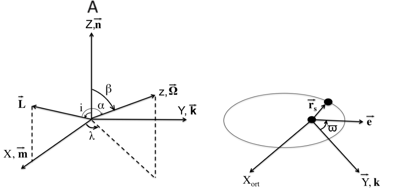
Figure 1.— Observer coordinate frame on the left, and a sketch of the orbital geometry on the right. See text for more details.

The vector towards the observer in the symmetry system of each star is

$$\boldsymbol{n}=\begin{pmatrix}-\sin\beta_{i}\\ 0\\ \cos\beta_{i}\\ \end{pmatrix}$$ (2)

To simulate the eclipse light curves we also need to know the relative stellar trajectory projected onto the plane of the sky. The projected position of the center of the secondary with respect to primary in the observer frame is given by

$${\bf R_{s}}=r_{s}\begin{pmatrix}-\cos i\sin(f+\varpi)\\ \cos(f+\varpi)\\ \sin i\sin(f+\varpi)\end{pmatrix}$$ (3)

where $r_{s}$ is the distance of the secondary star with respect to the primary and $f$ is the true anomaly (see Murray & Dermott 2000 for relation with other orbital parameters). Equation (3) fully determine the time evolution of ${\bf R_{s}}$ during the eclipse.

2.2. Shape of the stellar surface.

We now describe the variation of intensity of emission over the stellar surface due to the gravity darkening effect. Our results will be valid both for the primary and the secondary, so we will omit the subscript $i=p,s$ in this subsection.

First, we determine the geometry of the sky-projected disc by assuming the shape of the stellar surface to coincide with isopotential surfaces for the effective potential

$$\Phi_{\rm eff}(x,y,z)=-\frac{GM_{\star}}{\sqrt{x^{2}+y^{2}+z^{2}}}-\frac{1}{2}\Omega_{\star}^{2}(x^{2}+y^{2}),$$ (4)

as a function of coordinates in the ”symmetry” frame. Assuming slow rotation one can obtain the equation for the stellar surface in the form

$$\frac{x^{2}+y^{2}}{{\eta}^{2}}+z^{2}={R^{2}_{pol}},$$ (5)

where $R_{pol}$ is the polar radius of the star. Thus, because of the rotation stellar surface has an ellipsoidal shape with oblateness $\eta$ given by

$$\eta=\frac{R_{eq}}{R_{pol}}=1+\frac{R^{3}_{i}\omega^{2}_{i}}{2GM_{i}}=1+\frac{S}{2}.$$ (6)

Here the parameter S is related to the ratio of the rotation rate $\omega_{i}$ to the breakup rotation rate $\omega_{b}\equiv(GM_{\star}/R_{\star}^{3})^{1/2}$ at which the centrifugal force balances gravity at the stellar surface. Equation (5) can be re-written in polar coordinates as $r(\theta)=R_{pole}(1+S\sin^{2}\theta/2)$.

The actual angular velocity of stellar spin is calculated from the spectroscopically measured projected stellar rotation velocity $(v_{rot}\sin\beta)_{obs}$ as

$$\omega=\frac{(v_{rot}\sin\beta)_{obs}}{R_{eq}\sin\beta},$$ (7)

where we assumed $R_{eq}$ equal to the stellar radius quoted in the literature.

2.3. Temperature distribution over the stellar surface.

Because of rapid stellar rotation the brightness temperature of the stellar surface is not constant but obeys the von Zeipel (1924) law

$$T({\bf R})=T_{pol}\left[\frac{g_{\rm eff}({\bf R})}{g_{pol}}\right]^{\beta_{g}}=T_{pol}\psi({\bf R}),$$ (8)

where $T_{pol}$ is the value of $T$ at the stellar pole, $\beta_{g}$ is the gravity darkening power law index, ${\bf R}$ is the three-dimensional radius-vector from the stellar center to a point on the stellar surface, and $g_{\rm eff}$ is the local effective gravitational acceleration:

$${\bf g}_{\rm eff}({\bf R})=-\frac{GM_{\star}}{R^{3}}{\bf R}+\omega^{2}{\bf R_{\perp}}.$$ (9)

Here ${\bf R}_{\perp}={\bf R}-(\boldsymbol{\omega}\cdot{\bf R})/\omega$ is the distance to that point from the stellar spin axis, and $g_{pol}$ is the value of $g_{\rm eff}$ at the stellar pole, where $R_{\perp}=0$.

Conventional gravity darkening theory (von Zeipel 1924) predicts $\beta_{g}=0.25$. However, recent detailed theoretical calculations (Deupree 2011) of the latitudinal distribution of the effective temperature for rotating stars performed in the wide range of stellar masses (between 1.625 and 8 $M_{\odot}$) suggest a considerably weaker dependence of $T({\bf R})$ on $g_{\rm eff}$. We illustrate this point in Figure 2, where we plot the latitudinal distribution of the effective temperature for a particular stellar model from Deupree (2011) corresponding to a rotation parameter $S=0.09$. This distribution depends on stellar mass only weakly, meaning that it can be applied for DI Her components as well. One can see that equation (8) with $\beta_{g}=0.075$, which is considerably lower than $0.25$, provides excellent fit to these data.

On the observational side, interferometric measurements for rapidly rotating stars by Che et al. (2011) find $\beta_{g}\approx 0.146$ for 1.77$M_{\odot}$ star $\beta$ Cassiopeiae, having $v_{rot}\sin\beta\approx 75$ km s^-1 and $\beta_{g}\approx 0.19$ for 4.15$M_{\odot}$ star $\alpha$ Leo, rotating at $v_{rot}\sin\beta\approx 340$ km s^-1. Even though the latter is very similar in mass to the DI Her components, it spins much faster (spin parameter $S$ is almost an order of magnitude higher), making direct extrapolation to the DI Her case difficult. Despite these ambiguities, it is clear that both theoretically and observationally one typically infers $\beta_{d}<0.25$. In this work we have chosen to adopt $\beta_{g}=0.1$ more in line with the work of Deupree (2011).

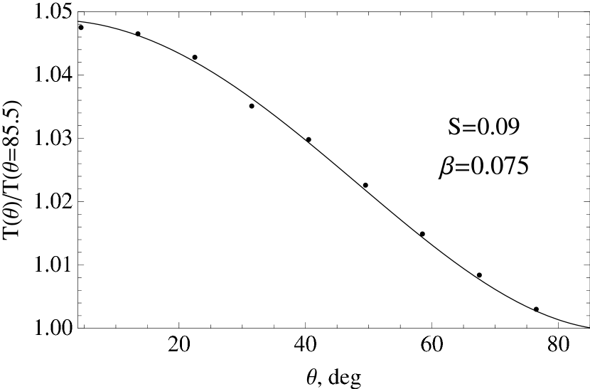
Figure 2.— Latitudinal distribution of the brightness temperature for a stellar model with rotation parameter $S=0.09$ (points; Deupree, 2010) fitted by a von Zeipel law (equation (8); solid line) with low value of $\beta_{g}=0.075$ that is close to $\beta_{g}=0.1$ used in this work.

2.4. Intensity distribution over the sky-projected disc.

Equations (8), (9) provide us with a simple expression for $T({\bf R})$ in the symmetry frame of a star, since ${\bf R}$ in this frame can be trivially derived from equation (5). However, for the purposes of eclipse lightcurve modeling we need to know the temperature distribution in the observer frame, projected onto the plane of the sky. In Appendix A we describe the relation between $(x_{i},y_{i},z_{i})$ and $(X,Y,Z)$ frames, which allows us to write the dimensionless function $\psi$ in equation (8) as $\psi({\bf R})=\psi(X,Y,Z(X,Y,\boldsymbol{\omega}_{i}))=\psi(X,Y,{\bf\omega}_{i})$ for each star. The dependence of $\psi$ on $\boldsymbol{\omega}_{i}$ is the key factor that allows us to use stellar photometry during eclipse to determine the spin orientation of the stars. Figure 3b,d illustrates the distribution of the brightness temperature over the stellar surface projected onto the sky plane.

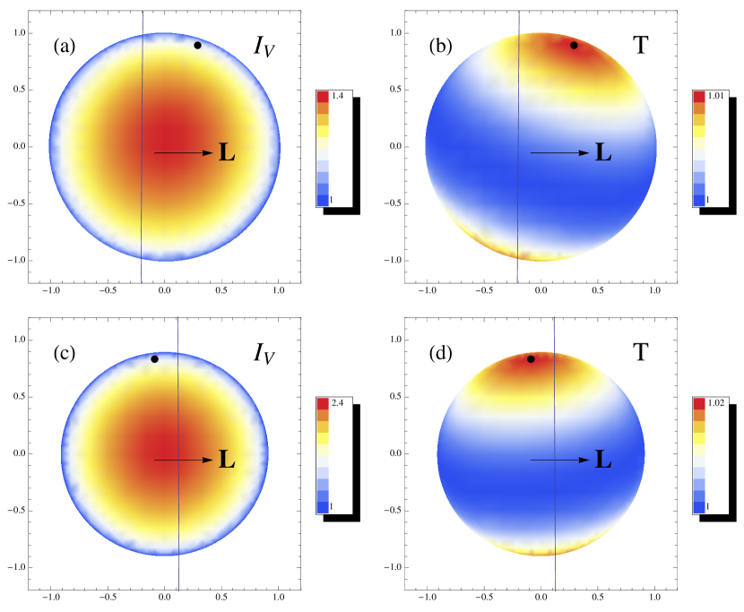
Figure 3.— Intensity distribution for the primary (a) and secondary (c) stars, and temperature distribution for the primary (b) and secondary (d). Calculations assume $\beta_{p}=70^{\circ}$, $\lambda_{p}=72^{\circ}$, $\beta_{s}=110^{\circ}$, $\lambda_{s}=-84^{\circ}$, $S=0.040$ for the primary star, $S=0.046$ for the secondary star, limb-darkening coefficient $c_{1}=0.35$ for the primary star, $c_{1}=0.64$ for the secondary star and von Zeipel parameter $\beta_{g}=0.1$. The dot on each plot indicates the position of the stellar pole. The blue line shows the trajectory of the center of the secondary (primary) star during primary (secondary) eclipse. The arrow shows the direction of the projected orbital angular momentum ${\bf L}$. Temperature distribution clearly illustrates gravity darkening. The intensity variation is large (tens of per cent) mainly because of the limb darkening effect, which is much larger than the gravity darkening.

Spectral density of the stellar radiation flux detected on Earth is

$$F_{\lambda}=\frac{1}{d^{2}}\int\limits_{S}I_{\lambda}(T_{pol}\psi(X,Y,\boldsymbol{\omega}))\Phi_{\lambda}(X,Y,\boldsymbol{\omega}){dXdY},$$ (10)

where $d$ is the distance to the system, $\Phi_{\lambda}$ is the limb-darkening law, and $I_{\lambda}(T)$ is the spectral intensity at a given temperature $T$. In this work we assume that $I_{\lambda}(T)=B_{\lambda}(T)$, where $B_{\lambda}(T)$ is a standard black-body radiation function. Thus, spectrum of each star is in general a multi-color blackbody, parametrized by $T_{pol}$ and $\psi$.

On the other hand, values of the effective temperature $T_{\star}$ for both stars quoted in the literature are obtained assuming that both stars radiate as pure blackbodies characterized by a single value of temperature, uniform across the stellar surface (Claret 2010). In that case the total bolometric flux is $F=L_{*}/(4\pi d^{2})=\sigma T^{4}_{eff}R^{2}_{*}/d^{2}$, where $L_{*}$ is the stellar luminosity. This assumption is not valid for rapidly rotating stars because of gravity darkening, and $T_{pol}$ cannot be taken equal to $T_{\star}$. To relate them we integrate equation (10) over all wavelengths to obtain the following expression for $T_{pol}$:

$$T_{pol}=T_{\star}\left[\frac{1}{\pi R^{2}_{*}}\int\limits_{S}\psi^{4}(X,Y,\boldsymbol{\omega})\Phi_{\lambda}(X,Y,\boldsymbol{\omega}){dXdY}\right]^{-1/4},$$ (11)

i.e. there is a correction depending on the orientation of stellar spin. This self-consistent derivation of $T_{pol}$ is an important part of our procedure which distinguishes it from the approach of Barnes (2009).

For simplicity the limb-darkening law in this work is assumed to be frequency- and spin-independent and have a simple functional form

$$\Phi_{\lambda}=1-c_{1}(1-\mu),$$ (12)

where $c_{1}$ is constant and $\mu$ is the cosine of the angle between the local normal ${\boldsymbol{\xi}}$ to the stellar surface and the observer’s line of sight: $\mu={\boldsymbol{\xi}}\cdot{\bf{n}}$. The total measured flux in the V band $F_{V}$ is obtained by additionally convolving $F_{\lambda}$ in equation (10) with $W_{\lambda}$ — the normalized transmission function for that band — over $\lambda$.

Figure 3a,c shows how the radiation intensity is distributed over the stellar surface for the two components of the DI Her system out of eclipse, when both gravity-darkening and limb-darkening are taken into account. It is obvious that limb-darkening has a much stronger effect on the intensity distribution than the gravity darkening, complicating measurement of the latter effect in the photometric data and determination of the spin orientation of the two stars. On the other hand, as long as the stellar spin axis is not aligned with our line of sight, the gravity darkening results in a non-axisymmetric brightness distribution with respect to our line of sight, unlike the limb darkening, which is axisymmetric. This helps one disentangle the two contributions in the photometric data.

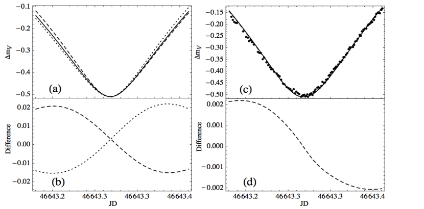
Figure 4.— (Left) Top panel shows simulated light curves of the secondary eclipse for the uniform temperature distribution (solid line), fast rotation (S=0.13) and two different secondary spin orientations - $\beta_{s1}=70^{\circ}$, $\lambda_{s1}=90^{\circ}$ (dashed line) and $\beta_{s2}=70^{\circ}$, $\lambda_{s2}=-100^{\circ}$ (dotted line) (primary star parameters are kept constant at $\beta_{p}=70^{\circ}$, $\lambda_{p}=72^{\circ}$). On the lower left panel the difference between simulated curves (dashed for the first case and dotted for the second one) and the case of uniform temperature distribution is given. For the first orientation dimmer regions are blocked first, with the opposite being true for the second one. (Right) Top panel shows simulated light curves for the uniform temperature distribution (dashed line) and actual DI Hercules parameters ($\beta_{p}=70^{\circ}$, $\beta_{s}=110^{\circ}$, $\lambda_{p}=72^{\circ}$, $\lambda_{s}=-84^{\circ}$, $S_{p}=0.040$, $S_{s}=0.046$). Dots correspond to observational data (secondary eclipse 7/13/1986). The differences between the theoretical lightcurves are hardly visible, so we visualize them on the lower panel (we do not show data point there as they would be off scale).

For simulating the light curves we need to calculate the flux blocked during the eclipse

$$I_{bl,i}(\boldsymbol{\omega},t)=\int H(X,Y,t)F_{V,i}(X,Y,\boldsymbol{\omega})dXdY,~{}~{}~{}i=p,s,$$ (13)

where $H(X,Y,t)$ equals 1, if the secondary (primary) star blocks starlight of the primary (secondary) at position $(X,Y)$, and 0 if not. Then the total flux observed on Earth is

$$I(\boldsymbol{\omega},t)=I_{p}+I_{s}-I_{bl,i}(\boldsymbol{\omega},t),$$ (14)

where $I_{p}$ and $I_{s}$ are the unblocked stellar fluxes, i.e. calculated from equation (13) with $H$ set to unity. During the eclipse $I_{bl,i}(\boldsymbol{\omega},t)$ changes because function $H$ varies with time across the surface of eclipsed star. In this work we take the surface (and frequency because of the finite bandwidth) integral in equation (13) using Monte Carlo technique.

Our lightcurve modeling procedure is illustrated in Figure 4, where in left panels we demonstrate the differences between the model assuming uniform distribution of the surface temperature and the models in which the effect of gravity darkening is fully taken into account. One can see that for relatively fast rotation ($S=0.13$ or $\omega=0.36\omega_{b}$) the difference between the uniform $T$ case and the gravity-darkened models is at the level of several per cent, which should be easily detectable in single-epoch observations.

In right panels of the same Figure we show the comparison between the uniform temperature case, the gravity-darkened model with spin angles resulting from our fits to the data (see §4). In this case $S\approx 0.04$, see Table 1, and the difference between the uniform and gravity-darkened models is very small, $\sim 10^{-3}$ mag. Thus, in the case of DI Her one would need very high-quality photometry (at the level of several $\times 10^{-4}$ mag) to detect gravity darkening-related asymmetries in the lightcurve shape.

3. Observational data and fitting procedure

3.1. Observations.

The dataset we use for determining spin orientation of the DI Her components consists of photoelectric V band measurements of this system using the 50-cm AZT-14 reflector at the Tien Shan Observatory of the Astrophysical Institute of Kazakhstan and the Zeiss-600 reflector at the Crimean Station of the Sternberg Astronomical Institute prepared in 2003–2008. The database also contains the photoelectric observations going further in the past by Semeniuk (1968), the 1968–-1978 observations by Martynov and Khaliullin (1980), the 1986–-1988 observations by Khodykin, Volkov, and Metlov, and the 2004 observations by Shugarov (see Kozyreva & Bagaev 2009 and the references there in). These observations use different instruments, which were not cross-calibrated. Our fitting uses 9 eclipses, 4 primary and 5 secondary. The photometric errors are unconstrained in all cases and we describe in §3.4 how we deal with this issue.

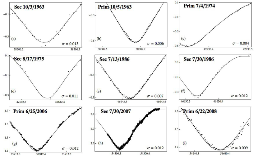
Figure 5.— Eclipse data used in our modeling with best fits overplotted. Horizontal axis is JD and the vertical one is apparent magnitude in the V band for every eclipse. Labels indicate the date of eclipses and the adopted noise levels.

3.2. Time evolution of the system.

High mass, rapid rotation and relative proximity of the stars in DI Her system drive rapid evolution of the spin orientations for both components. In Appendix B we derive equations that describe evolution of the stellar spins and orbital elements of the system. In particular, we show there that stellar spins in DI Her can rotate by more than $100^{\circ}$ within a century, see equation (B14). This evolution obtained by integrating equations from Appendix B over time is illustrated in Figure 6.

Figure 6.— Evolution of the DI Her spin orientation (angles $\beta$ and $\lambda$) for both stars and the inclination $i$ of the system both on short (left) and long (right) time intervals. Dashed vertical lines correspond mark the locations of eclipses used in our modeling. Variation of spin angles $\beta_{i}$ and $\lambda_{i}$, $i=p,s$ are very significant.

This Figure clearly demonstrates that spin orientation of the DI Her components significantly changes over the time span of our full dataset. On one hand this complicates the eclipse fitting, but on the other hand it provides us with a unique opportunity to use the signatures of this variation of stellar spins in eclipse modeling on long time intervals.

In this regard our procedure of eclipse simulation uses somewhat different strategy that the one proposed by Barnes (2009): instead of using high-accuracy photometric data in a single epoch, which provides sensitivity to spin orientation only through the shape of the eclipse lightcurve, we use low-accuracy photometry obtained at different epochs, which allows for an additional effect of the current spin orientation of DI Her on the fitting procedure — through the time evolution of ${\bf\omega}_{i}$.

3.3. Evolution of $v_{rot}\sin\beta$.

Precession of stellar spins causes evolution of $v_{rot,i}\sin\beta_{i}$ ($i=p,s$) on long time interval, which can be compared with past measurements. We took the values of $v_{rot,i}\sin\beta_{i}$ from Albrecht et al. (2009), who compiled measurements from different epochs starting in 1948. Figure (10) shows these data. Unfortunately, the large (or completely undetermined as in the case of 1948 data point) uncertainties of these measurements do not allow us to infer the values of $\beta_{p}$ and $\beta_{s}$ from these data alone. However, even the weak constraints based on these measurements turn out being quite useful.

We will use the fact that based on these data $v_{rot}\sin\beta$ is currently increasing for both primary and secondary components. As $v_{rot}$ is constant this can only be due to $\sin\beta_{j}$ increasing in time. From the evolution equation (B20) we find the expression for the derivative of $\sin\beta_{j}$ ($j=p,s$):

$$\frac{d\sin\beta_{j}}{dt}=3\Omega_{P,j}\sin i\sin\lambda_{j}\cos\beta_{j}(\cos i\cos\beta_{j}+$$

$$+\sin i\sin\beta_{j}\cos\lambda_{j})\approx\frac{3}{2}\Omega_{P,j}\sin^{2}i\sin(2\lambda_{j})\cos\beta_{j},$$ (15)

where $\Omega_{P,j}$ is the frequency describing spin precession caused by the rotation-induced stellar oblateness (see equation (B14)) and the approximation holds for $i\approx 90^{\circ}$. From the Rossiter-McLaughlin measurements of Albrecht et al. (2009) we know that $\sin 2\lambda_{j}$ is positive for the primary and negative for the secondary. Thus, it follows from the current time derivatives of $\sin\beta_{p,s}$ that $\beta_{p}$ must be less than $90^{\circ}$ while $\beta_{s}$ should be greater than $90^{\circ}$. We use this information to help constrain stellar spin orientation in §4.

3.4. Photometric fitting procedure.

The specific parameters of DI Herculis that we used in simulations are summarized in Table 1. To keep things simple we have only varied the most important unknown quantities — the angles $\beta_{p}$ and $\beta_{s}$. Given the quality of the data we expect that fitting for extra parameters in our model would result in too many degeneracies between the different model variables.

We integrate back in time the evolution equations for spin and orbital parameters (Appendix B) starting from 15 July, 2008, which is set as the initial point in our calculations. The angles $\beta_{p}$ and $\beta_{s}$ that we vary correspond to this epoch. The other two angles specifying spin orientation were fixed at $\lambda_{p}=72^{\circ}$ and $\lambda_{s}=-84^{\circ}$ based on the Rossiter-McLaughlin measurements of Albrecht et al. (2011).

To obtain better eclipse fits we had to introduce quite different limb-darkening coefficients for the two components, which, given the proximity of stellar masses in DI Her, suggests that our data are affected by some systematic effects. Nevertheless, given that the limb darkening only weakly affect the non-axisymmetric surface brightness distribution due to gravity darkening (see §2.4), the actual values of limb-darkening coefficients are not so important.

We constrain DI Her spin orientation as follows. For each pair $\beta_{p}$, $\beta_{s}$ we compute

$$\chi^{2}=\frac{1}{N}\sum\limits_{j=1}^{9}\sum\limits_{i=1}^{N_{j}}\frac{(I(t_{i})-I^{j}_{obs}(t_{i}))^{2}}{\sigma^{2}_{i}},$$ (16)

where index $j$ runs through all 9 eclipses, $i$ runs through the number of data points per each lightcurve (total of $N_{j}$ for $j$-th eclipse), $N=\sum_{j=1}^{9}N_{j}$ is the total number of data points, $I(t)$ is given by equation (14), $I^{j}_{obs}(t)$ is the observed intensity, and $\sigma_{i}$ is the variance. The best fit values of $\beta_{p}$ and $\beta_{s}$ are determined by finding the minimum of $\chi^{2}$ over a large two-dimensional grid of values of these angles. We use only the eclipses with well-defined minima. We did not try to match theoretical and observational eclipse minima with our direct backward integration in time and instead just shift theoretical curves horizontally by small amount at each epoch for a better fit.

Figure 7.— Sensitivity of spin angle determination to the noise level assumed for the data. We simulate the primary eclipse lightcurve using theoretical prescription (14) with a given level of the Gaussian noise $\sigma$ for a fixed spin angle $\beta_{p}=40^{\circ}$ for the primary. We vary only this angle in our $\chi^{2}$ fitting ($\beta_{s}=40^{\circ}$, $\lambda_{p}=72^{\circ}$ and $\lambda_{s}=-84^{\circ}$ are constant here) just to illustrate that large noise level does not allow us to constrain system parameters, while $\sigma\approx 0.01$ mag yields the correct orientation of the system.

As mentioned before, the errorbars for our dataset are not constrained, so we employed the following procedure to estimate them. First, we took all $\sigma_{i}$ to be constant and run our minimization procedure to find the best fit values of $\beta_{p}$ and $\beta_{s}$. Second, for each out of 9 eclipses we measure the scatter $\sigma_{j}$ of the observational data points around the model lightcurve computed assuming these particular values of $\beta_{p}$ and $\beta_{s}$. This provides us with 9 different values of $\sigma_{j}$ (indicated in panels in Figure 5 for each eclipse), which we use as error estimates in equation (16). Typical values of $\sigma_{j}$ found using this procedure are $\sim 0.01$ mag. We then perform the final $\chi^{2}$ minimization adopting these values of $\sigma_{j}$ as error estimates for corresponding eclipses. In this approach all data points corresponding to $j$-th eclipse have a single value of the photometric error equal to $\sigma_{j}$.

We test the performance of our fitting algorithm by applying it to a simulated dataset in a simplified setup. We calculate a theoretical primary eclipse lightcurve including the gravity darkening effect and assuming a binary with physical parameters ($M_{\star},R_{\star},T_{\star}$, etc.) of the DI Her (in particular with $S\approx 0.04$ for both stars). We take somewhat arbitrarily $\beta_{p}=40^{\circ}$, $\beta_{s}=40^{\circ}$, $\lambda_{p}=72^{\circ}$ and $\lambda_{s}=-84^{\circ}$. We then add some random Gaussian noise with variance $\sigma$ to this simulated lightcurve. For this test we assume $\beta_{s}$, $\lambda_{p}$ and $\lambda_{s}$ to be known and try to measure the value of only $\beta_{p}$ using our procedure. As a consequence, we need to perform only one-dimensional minimization over $\beta_{p}$.

The results of this exercise are shown in Figure 7, where we show $\chi^{2}$ curves for two different values of the noise variance $\sigma$: $0.01$ mag and $0.03$ mag. One can see that for $\sigma=0.03$ mag our parameter estimation procedure cannot recover the adopted value of $\beta_{p}$ — the $\chi^{2}$ distribution has very extended flat bottom which does not lead to a useful constraint on $\beta_{p}$. However, for $\sigma=0.01$ mag our procedure works reasonably well and the minimim of $\chi^{2}$ is close to the input value of $\beta_{p}=40^{\circ}$. Since the simulated lightcurve was computed for realistic physical parameters of the DI Her and the noise levels for individual eclipses in real data $\sigma_{j}$ are indeed $\sim 0.01$ mag we expect that our parameter estimation for a real dataset should be able to determine real $\beta_{p}$ and $\beta_{s}$ with reasonable accuracy.

4. Results

Table 1DI Herculis parameters

Parameter	Primary	Secondary
Stellar radius ($R_{\odot}$)	2.68	2.48
Stellar mass ($M_{\odot}$)	5.15	4.52
Von Zeipel’s parameter $\beta_{g}$	0.1	0.1
Effective temperature (K)	17300	15400
$v_{rot}\sin\beta$ (${\rm km\cdot s^{-1}}$)	108	116
$c_{1}$	0.35	0.64
$\lambda$ (∘)	72	-84
Derived parameters
$\beta$ (∘)	$62\pm 17$	$90\leq\beta_{s}\leq 110$
$\omega R$ (${\rm km\cdot s^{-1}}$)	112	124
S	0.040	0.046

We display the results of our fitting procedure in Figure 8, which shows a map of $\chi^{2}$ distribution as a function of $\beta_{p}$ and $\beta_{s}$. We see that in the broad region near the minimum the value of $\chi^{2}$ is almost constant, which precludes us from deriving accurate values of the spin angles from the eclipse analysis alone. While the angle $\beta_{p}$ for the primary is constrained to lie in the range $30^{\circ}-70^{\circ}$, the eclipse photometry alone does not set a reasonable limit on $\beta_{s}$: we can only say that it should lie within $50^{\circ}-140^{\circ}$ interval. This difference is caused by the different noise levels for primary and secondary eclipses: 4 out of 5 secondary eclipses used have $\sigma_{j}>0.01$ mag, while 3 out of 4 primary eclipses have $\sigma_{j}<0.01$ mag (one primary eclipse has $\sigma_{j}=0.004$ mag). As we demonstrated in previous section, large values of $\sigma_{j}$ significantly deteriorate the performance of our parameter estimation procedure (see Figure 7), which is apparently the case for secondary eclipses, during which the lightcurve is most sensitive to $\beta_{s}$.

To obtain a better measurement of these angles we apply two additional constraints. One of them uses the observed precession rate $\dot{\omega}_{obs}=1^{\circ}.24\pm 0^{\circ}.18/100$ yr (Martynov & Khaliullin 1980). The apsidal precession rate $\dot{\omega}$ depends on $\beta_{p,s}$ since it contains a contribution due to the rotation-induced stellar quadrupole, see equation (B18), while the latter depends on these angles according to equation (7). We show the constraint on the apsidal precession rate (corresponding to 1$\sigma$ deviation) by yellow curve in Figure 8, where the analytical estimate of $\dot{\omega}$ is obtained using (B18).

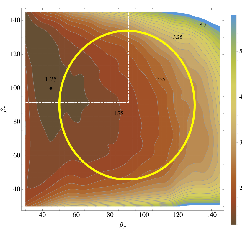
Figure 8.— $\chi^{2}$ distribution over all eclipses. The black dot shows the global minimum of $\chi^{2}$ distribution within the considered range of $\beta_{p}$ and $\beta_{s}$. The yellow ellipse shows the constrain coming from the precession rate corresponding to 1$\sigma$ level, where the analytical estimate of $\dot{\omega}$ is obtained using (B18). Evolution of $v_{rot}\sin\beta$ at present time additionally constrains $\beta_{p}<90^{\circ}$, $\beta_{s}>90^{\circ}$ (represented by white dashed lines).

Figure 9.— Probability density distribution for $\beta_{p}$, $\beta_{s}$ obtained by combining the eclipse fitting and the constraint on the precession rate. Yellow thick contour gives $1\sigma$ level. The best fit values of spin angles that we derive from this map are $\beta_{p}=62^{\circ}\pm 17^{\circ}$ and $\beta_{s}=90^{\circ}\pm 20^{\circ}$ (yellow thin contour). The white dashed curve additionally shows the $v_{rot}\sin\beta$ evolution constraint, see §3.3.

To obtain approximate values and the error bars of the angles $\beta_{p}$ and $\beta_{s}$ based on the eclipse fitting and the measurement $\dot{\omega}$, we first construct the photometric probability distribution of these angles using the $\chi^{2}$ map from Figure 8. We then convolve it with the distribution of $\beta_{p}$ and $\beta_{s}$ (assumed to be a two-dimensional Gaussian) based on the $\dot{\omega}$ measurement of Albrecht et al. (2009). The map of the resultant probability density distribution is shown in Figure 9. From this map we find $\beta_{p}=62^{\circ}\pm 17^{\circ}$ and $\beta_{s}=90^{\circ}\pm 20^{\circ}$, where the errors correspond to 1-$\sigma$ uncertainty. Comparing with Figure 8 we see that $\beta_{s}$ is constrained essentially purely by the $\dot{\omega}$ measurement, with photometric data not being useful. At the same time, for the primary angle $\beta_{p}$ the photometric data do result in a meaningful measurement, reducing $\beta_{p}$ from the value suggested by $\dot{\omega}$ alone and lowering error considerably.

Another constraint on spin orientation is based on the evolution of $v_{rot}\sin\beta$ for both components (see §3.3) and is illustrated by the white dashed line in Figures 8 & 9. This constraint is most important for the spin orientation of the secondary as it excludes $\beta_{s}<90^{\circ}$ from the consideration. As a result, we come up with a refined measurement of $\beta_{s}=100^{\circ}\pm 10^{\circ}$.

Figure 10.— Evolution of $V_{j}\sin\beta_{j}$ for both stars for derived angles $\beta_{p}=62^{\circ}$, $\beta_{s}=100^{\circ}$ (a) and for another set $\beta_{p}=55^{\circ}$, $\beta_{s}=120^{\circ}$ (b). In both cases $\lambda_{p}=70^{\circ}$ and $\lambda_{s}=-76^{\circ}$. Solid and dashed curves correspond to theoretical curves for primary and secondary stars. Circles and triangles with errorbars (when available) represent the measurements for secondary and primary, correspondingly, taken from Albrecht et al. (2009). It shows that the derived $\beta_{s}$ from photometrical analysis does not provide the best fit for $V_{s}\sin\beta_{s}$ evolution.

Figure 5 shows model lightcurves for these best fit values of $\beta_{p}$ and $\beta_{s}$ for all eclipses used in this work. One can clearly see the existence of some features in the lightcurves that remain unfit by our gravity-darkened model, especially at the midpoint of some eclipses. These are likely artefacts of the measurements using different instruments and at different locations.

5. Discussion and conclusions

In this work we developed a method for determining full three-dimensional spin-orbit geometry of an eclipsing binary system with rapidly rotating components. The idea behind this method lies in using the gravity darkening effect and its influence on the properties of the photometric lightcurve of the system. Using this method, coupled with two additional constraints — the value of the apsidal precession rate of the system and the evolution of spectroscopically determined projection of the stellar rotation speed — we were able to provide a reasonable measurement of the projections of stellar spins onto our line of sight in the eclipsing binary DI Her.

A very similar technique based on the gravity darkening effect has already been employed to infer the spin-orbit orientation in a planetary system KOI-13.01, which contains a rapidly rotating ($v_{rot}\sin\beta=65\pm 10$ km s^-1) intermediate mass star (Szabó et al. 2011; Barnes et al. 2011). This measurement used several eclipses (transits) obtained over a short time span, as opposed to our procedure that uses data spread over a long time interval. In the case of Barnes et al. (2011) the exquisite photometric accuracy of Kepler allowed derivation of a rather tight constraint on the spin orientation of the host star in KOI-13.01 system, something that we cannot accomplish with our low-quality multi-epoch photometry. The same kind of photometric accuracy ($\sim 10^{-4}$ mag) would provide us with a much better constraint on the DI Her orientation angles even with single epoch data, see §2.4.

Modeling the gravity darkening-modified eclipse lightcurves in binary stars is not an easy task because each component of the binary covers large portion of the disk of another. This requires integration of the intensity distribution over a large fraction of the stellar surface, which naturally gives rise to degeneracies between different parameters of the system, making it difficult to determine stellar spin orientation. On the other hand, in the case of planetary transits planet covers only a small fraction of the stellar surface so that the eclipse lightcurve can be directly related to the one-dimensional run of stellar surface temperature asymmetries. The latter can be much more easily modeled via the gravity darkening effect to infer the system orientation.

As of now there is no good explanation for the strong spin-orbit misalignment of DI Her (Albrecht et al. 2010). It could be primordial, resulting from an interaction between the stars and the disk from which they formed, which would require some yet unknown mechanism to get accomplished. Alternatively, the system may contain a third body in a wider orbit as suggested by Kozyreva & Bagaev (2009) based on timing of eclipses over a long time span. If the orbit of that body is highly inclined with respect to the orbit of the inner two stars then the Lidov-Kozai mechanism (Lidov 1962; Kozai 1962) may be invoked to explain the spin-orbit misalignment in DI Her. This idea clearly requires further investigation, but we will mention that Lidov-Kozai cycles with tidal dissipation are often considered responsible (Fabrycky & Tremaine 2007) for the spin-orbit misalignments inferred in many extrasolar planetary systems (Albrecht et al. 2012).

It is interesting that recently started BANANA project (Albrecht et al. 2011) focusing on the Rossiter-McLaughlin measurements in binaries containing rapidly spinning stars reported close spin-orbit alignment for the primary star in the NY Cep system, which is similar to DI Her in many respects. On the other hand, there are other eclipsing binary systems such as AS Camelopardalis, which exhibit anomalously slow apsidal precession, similar to DI Her (Pavlovski et al. 2011). If it is the spin-orbit misalignment that is causing the anomalous precession in AS Camelopardalis then the photometric method developed in this work and Barnes (2009) may be used to constrain the system orientation (although the measured projected rate in this system is not very high, $\approx 15$ km s^-1 for the primary component).

Appendix A Geometry of the sky–projected stellar disc

In this section we will derive the relation between the coordinates of a given point on the stellar surface in the observer and symmetry frames. Normal $\boldsymbol{\xi}$ to the stellar surface at a point $(x,y,z)$ in the symmetry frame is ($|\boldsymbol{\xi}|\neq 1$)

$$\boldsymbol{\xi}=\left(\frac{x}{{\eta}^{2}},\frac{y}{{\eta}^{2}},z\right)$$ (A1)

Because of the rotation-induced distortion the sky-plane projected stellar shape is not circular. The last visible points on the stellar surface for the observer are given by the following equation

$${\bf n}\cdot{\boldsymbol{\xi}}=0$$ (A2)

where $\bf n$ is a unit vector towards the observer given by equation (2). It results in the following equations:

$$z=\frac{\tan{\beta}}{\eta^{2}}x,~{}~{}~{}~{}~{}~{}~{}~{}~{}~{}\frac{x^{2}}{\eta^{2}}\left(1+\frac{\tan^{2}\beta}{\eta^{2}}\right)+\frac{y^{2}}{\eta^{2}}=R^{2}_{pol}$$ (A3)

Equations (A3) give us the ”critical line” of the last visible points on the stellar surface (where $\boldsymbol{\xi}$ lies in the sky plane) in the symmetry system. It defines the shape of the visible stellar disk. To obtain the coordinates in observer frame the corresponding coordinate transformation should be made:

$$x=\cos\beta x_{0}-\sin\beta Z,~{}~{}~{}~{}~{}~{}~{}~{}z=\sin\beta x_{0}+\cos\beta Z,$$ (A4)

where we defined

$$x_{0}=\cos\lambda X+\sin\lambda Y,~{}~{}~{}~{}~{}~{}~{}~{}y_{0}=-\sin\lambda X+\cos\lambda Y.$$ (A5)

So the equation for the critical line written in the observer frame is

$$Z=\frac{x_{0}(\eta^{-2}-1)\tan\beta}{1+\eta^{-2}\tan^{2}\beta}\equiv x_{0}\tan p,$$ (A6)

$$\frac{x^{2}_{0}}{\cos^{2}\beta+\eta^{-2}\sin^{2}\beta}+y^{2}_{0}=\eta^{2}R^{2}_{pol}.$$ (A7)

where $p$ is defined by equation (A6). In coordinates $(x_{0},y_{0},Z)$ the stellar surface is described by

$$\frac{y^{2}_{0}+(\cos(\beta)x_{0}-\sin(\beta)Z)^{2}}{\eta^{2}}+\left(\sin(\beta)x_{0}+\cos(\beta)Z\right)^{2}=R^{2}_{pol},$$ (A8)

from which one can find $Z$ in terms of $X$ and $Y$. The solution to the resulting quadratic is

$$Z=x_{0}\tan p+\frac{\eta^{-1}\sqrt{det}}{\cos^{2}\beta+\eta^{-2}\sin^{2}\beta}$$ (A9)

where the expression for the determinant $det$ is

$${det}=-\left[x^{2}_{0}+\left(y^{2}_{0}-\eta^{2}R^{2}_{pol}\right)\left(\cos^{2}\beta+\frac{\sin^{2}\beta}{\eta^{2}}\right)\right].$$ (A10)

It can be easily checked that the condition $det=0$ coincides with the equation for the critical line, so in the region interior to this line $det>0$. We choose the positive root of the determinant (the negative root represents the invisible side of the star as seen from Earth, see Barnes (2009). So if $(X,Y,0)$ is the point on the sky-projected stellar disc then ${\bf R}(X,Y)=(X,Y,Z(X,Y))$ represents the full three-dimensional coordinates of the point on the stellar surface right above $(X,Y,0)$ in the observer frame.

In general, to find coordinates $(x,y,z)$ of a point on the stellar surface in the symmetry frame corresponding to a point $(X,Y)$ projected onto the sky plane one has to compute $x_{0}$ and $y_{0}$ via equation (A5), determine $Z$ using (A9)-(A10), obtain $x$ and $z$ from equation (A4), and finally determine $y$ from equation (5).

Appendix B Time evolution

Here we derive equations that describe the evolution of the binary orbit and spin orientation of its components. We denote ${\bf L}=L{\bf l}$, ${\bf S}_{j}=S_{j}{\bf s}_{j}$, $j=p,s$ the orbital angular momentum and spin angular momenta of the two stars respectively, $|{\bf l}|=|{\bf s}_{j}|=1$. Here

$$L=\mu\Omega_{K}a^{2}\sqrt{1-e^{2}},~{}~{}~{}S_{j}=I_{j}\omega_{j}=\eta_{j}M_{j}R_{j}^{2}\omega_{j},$$ (B1)

where $M_{j}$, $R_{j}$, $\omega_{j}$ are the masses, radii and spin angular frequencies of the two stars, $\eta_{j}$ are constants determining their moments of inertia, $\mu=M_{p}M_{s}/(M_{p}+M_{s})$ is the reduced mass, $a$, $e$, and $\Omega_{K}=[G(M_{p}+M_{s})/a^{3}]^{1/2}$ are the semi-major axis, eccentricity and mean orbital frequency. We introduce unit vector ${\bf n}$ from the system’s barycenter to the observer and direct a Cartesian coordinate system in the directions ${\bf n}$, ${\bf m}$, ${\bf k}$ where

$${\bf k}=\frac{{\bf n}\times{\bf l}}{\sin i},~{}~{}~{}{\bf m}={\bf k}\times{\bf n}=\frac{1}{\sin i}[{\bf l}-{\bf n}({\bf l}\cdot{\bf n})],$$ (B2)

where $i$ is the inclination of the system, $\cos i=({\bf l}\cdot{\bf n})$, see Figure 1.

Orientation of ${\bf s}_{j}$ is conventionally given by the three angles $\alpha_{j}$, $\beta_{j}$, $\gamma_{j}$ between each of ${\bf s}_{j}$ and vectors ${\bf l}$, ${\bf n}$, and ${\bf k}$ correspondingly, i.e.

$$\cos\alpha_{j}=({\bf s}_{j}\cdot{\bf l}),~{}~{}~{}\cos\beta_{j}=({\bf s}_{j}\cdot{\bf n}),~{}~{}~{}\cos\gamma_{j}=({\bf s}_{j}\cdot{\bf k}).$$ (B3)

Then it is easy to show that

$${\bf s}_{j}=\cos\beta_{j}{\bf n}+\frac{\cos\alpha_{j}-\cos i\cos\beta_{j}}{\sin i}{\bf m}+\cos\gamma_{j}{\bf k}.$$ (B4)

Observationally, it is also convenient to introduce angle $\lambda_{j}$ between the projection ${\bf s}_{\perp,j}=[{\bf s}_{j}-{\bf n}({\bf s}_{j}\cdot{\bf n})]/\sin\beta_{j}$ of ${\bf s}_{j}$ onto the sky plane and the projection ${\bf m}$ of vector ${\bf l}$ onto the same plane: $\cos\lambda_{j}=({\bf s}_{\perp,j}\cdot{\bf m})$. This is the angle which is measured by the Rossiter-McLaughlin effect. One can easily show that these four angles are related via

$$\cos\alpha_{j}=\cos i\cos\beta_{j}+\sin i\sin\beta_{j}\cos\lambda_{j},~{}~{}~{}~{}~{}\cos\gamma=\sin\lambda\sin\beta.$$ (B5)

Thus, knowing $\lambda_{j}$, $\beta_{j}$ and $i$ one can immediately obtain $\alpha_{j}$ from these expressions.

Orientation of the orbital ellipse in the plane of the orbit is given by the eccentricity vector ${\bf E}=e{\bf e}$ which points from the main focus to the pericenter. Given that direction defined by vector ${\bf k}$ is the direction of the line of nodes we identify the angle between ${\bf k}$ and ${\bf e}$ as the longitude of the periastron $\omega$ and write

$${\bf e}=\cos\omega{\bf k}+\sin\omega({\bf l}\times{\bf k}).$$ (B6)

Stellar asphericity due to rotation and tides as well as relativistic effects lead to evolution of ${\bf l}$, ${\bf e}$, and ${\bf s}_{j}$ described by the following equations (Barker & O’Connell 1975):

$$\dot{\bf l}={\bf\Omega}_{L}\times{\bf l},~{}~{}~{}~{}~{}~{}\dot{\bf e}={\bf\Omega}_{L}\times{\bf e},~{}~{}~{}~{}~{}~{}\dot{\bf s}_{j}={\bf\Omega}_{S,j}\times{\bf s}_{j},$$ (B7)

where

$${\bf\Omega}_{L}=\left(\Omega_{E}+\sum\limits_{j=s,p}\Omega_{T,j}\right){\bf l}+\sum\limits_{j=s,p}\Omega_{Q,s}\left[\cos\alpha_{j}{\bf s}_{j}+\frac{1-5\cos^{2}\alpha_{j}}{2}{\bf l}\right],$$ (B8)

$${\bf\Omega}_{S,j}=\Omega_{G,j}{\bf l}+\Omega_{P,j}\left({\bf s}_{j}-3\cos\alpha_{j}{\bf l}\right)\approx\Omega_{P,j}\left({\bf s}_{j}-3\cos\alpha_{j}{\bf l}\right).$$ (B9)

Here different contributions to precession rates are denoted as follows (Barker & O’Connell 1975; Claret et al 2010): orbital Einstein precession

$$\Omega_{E}=\dot{\omega}_{\rm GR}=\frac{3G\Omega_{K}(M_{s}+M_{p})}{c^{2}a(1-e^{2})}\approx 2.35^{\circ}/100~{}\mbox{yr},$$ (B10)

orbital precession caused by stellar quadrupole due to tidal distortions ($k_{2,j}$ are introduced below)

$$\Omega_{T,j}=15k_{2,j}\Omega_{K}\frac{M_{r}}{M_{j}}\left(\frac{R_{j}}{a}\right)^{5}\frac{8+12e^{2}+e^{4}}{8(1-e^{2})},~{}~{}~{}r\neq j,$$ (B11)

$$\Omega_{T,p}\approx 0.69^{\circ}/100~{}\mbox{yr},~{}~{}~{}\Omega_{T,s}\approx 0.63^{\circ}/100~{}\mbox{yr},$$

orbital precession due to rotation-induced stellar quadrupole

$$\Omega_{Q,j}=-\frac{3}{2}\frac{G(M_{p}+M_{s})J_{2,j}}{\Omega_{K}a^{5}(1-e^{2})^{2}}=-k_{2,j}\frac{M_{p}+M_{s}}{M_{j}}\frac{\omega_{j}^{2}}{\Omega_{K}(1-e^{2})^{2}}\left(\frac{R_{j}}{a}\right)^{5}$$ (B12)

$$\Omega_{Q,p}\approx-\frac{2.1^{\circ}/100~{}\mbox{yr}}{(\sin\beta_{p})^{2}}s^{-1},~{}~{}~{}\Omega_{Q,s}\approx-\frac{2.2^{\circ}/100~{}\mbox{yr}}{(\sin\beta_{s})^{2}}s^{-1},$$

geodetic spin precession

$$\Omega_{G,j}=\frac{G\Omega_{K}\mu(4+3M_{r}/M_{j})}{2c^{2}a(1-e^{2})},~{}~{}~{}j\neq r,$$ (B13)

$$\Omega_{G,p}\approx 0.61^{\circ}/100~{}\mbox{yr},~{}~{}~{}\Omega_{G,s}\approx 0.69^{\circ}/100~{}\mbox{yr},$$

and the spin precession caused by rotation-induced stellar oblateness

$$\Omega_{P,j}=\frac{GM_{p}M_{s}J_{2,j}}{2I_{j}\omega_{j}a^{3}(1-e^{2})^{3/2}}=\frac{k_{2,j}}{3\eta_{j}}\frac{M_{r}}{M_{j}}\frac{\omega_{j}}{(1-e^{2})^{3/2}}\left(\frac{R_{j}}{a}\right)^{3},~{}~{}~{}r\neq j,$$ (B14)

$$\Omega_{P,p}\approx\frac{136.6^{\circ}/100~{}\mbox{yr}}{\sin\beta_{p}},~{}~{}~{}\Omega_{P,s}\approx\frac{168.6^{\circ}/100~{}\mbox{yr}}{\sin\beta_{s}}s^{-1},$$

In equations (B11), (B12), (B14) $k_{2,j}$ is the apsidal motion constant related to stellar rotation-induced quadrupole moment constant $J_{2,j}$ via

$$k_{2,j}=\frac{3}{2}\frac{J_{2,j}}{R_{j}^{2}}\left(\frac{\omega_{b,j}}{\omega_{j}}\right)^{2},~{}~{}~{}\omega_{b,j}\equiv\left(\frac{GM_{j}}{R_{j}^{3}}\right)^{1/2},$$ (B15)

with $\omega_{b,j}$ being the breakup angular frequency. Numerical estimates assume $k_{2,j}\approx 0.008$ (Claret et al. 2010) and the moment of inertia constant $\eta_{j}=0.063$ (Claret & Gimenez 1989). Given that $\Omega_{G,j}\ll\Omega_{P,j}$ we dropped geodetic contribution in equation (B9).

Differentiating relation $\cos i=({\bf l}\cdot{\bf n})$ with respect to time and using equations (B2), (B3), (B7), and (B8) one obtains

$$\dot{i}=-\frac{\dot{\bf l}\cdot{\bf n}}{\sin i}={\bf\Omega}_{L}\cdot{\bf k}=\sum\limits_{j=p,s}\Omega_{Q,j}\cos\alpha_{j}\cos\gamma_{j}.$$ (B16)

Because of precession of ${\bf l}$ vectors ${\bf k}$ and ${\bf m}$ vary in time. Differentiating equations (B2) with respect to time and using (B3), (B7), and (B8) their evolution is governed by equations

$$\dot{\bf k}=\frac{{\bf m}}{\sin^{2}i}\sum\limits_{j=p,s}\Omega_{Q,j}\cos\alpha_{j}\left(\cos i\cos\alpha_{j}-\cos\beta_{j}\right),~{}~{}~{}~{}~{}~{}~{}\dot{\bf m}=\frac{\bf k}{\sin^{2}i}\sum\limits_{j=p,s}\Omega_{Q,j}\cos\alpha_{j}\left(\cos\beta_{j}-\cos i\cos\alpha_{j}\right),$$ (B17)

Next, we differentiate $\cos\omega=({\bf e}\cdot{\bf k})$ as well as each of the relations (B3) with respect to time and transform them using equations (B2)-(B4), (B6)-(B9), (B16) and (B17). As a result we arrive at the following expressions:

$$\dot{\omega} = -\frac{(\dot{\bf e}\cdot{\bf k})+({\bf e}\cdot\dot{\bf k})}{\sin\omega}$$ (B18)

$$= =\Omega_{E}+\sum\limits_{j=p,s}\left\{\Omega_{T,j}+\frac{\Omega_{Q,j}}{\sin^{2}i}\left[\cos\alpha_{j}(\cos\alpha_{j}-\cos i\cos\beta_{j})+\sin^{2}i\frac{1-5\cos^{2}\alpha_{j}}{2}\right]\right\},$$

$$\dot{\alpha}_{j} = -\frac{(\dot{\bf l}\cdot{\bf s}_{j})+({\bf l}\cdot\dot{\bf s}_{j})}{\sin\alpha_{j}}$$ (B19)

$$= -\Omega_{Q,r}\frac{\cos\alpha_{r}}{\sin i\sin\alpha_{j}}\left[\cos\gamma_{r}(\cos i\cos\alpha_{j}-\cos\beta_{j})-\cos\gamma_{j}(\cos i\cos\alpha_{r}-\cos\beta_{r})\right],~{}~{}~{}j\neq r,$$

$$\dot{\beta}_{j} = -\frac{(\dot{\bf s}_{j}\cdot{\bf n})}{\sin\beta_{j}}=3\Omega_{P,j}\frac{\sin i\cos\gamma_{j}\cos\alpha_{j}}{\sin\beta_{j}},$$ (B20)

$$\dot{\gamma}_{j} = -\frac{(\dot{\bf k}\cdot{\bf s}_{i})+({\bf k}\cdot\dot{\bf s}_{i})}{\sin\gamma_{i}}$$ (B21)

$$= -\frac{\cos\alpha_{j}-\cos i\cos\beta_{j}}{\sin^{3}i\sin\gamma_{j}}\sum\limits_{r=s,p}\Omega_{Q,r}\cos\alpha_{r}(\cos i\cos\alpha_{r}-\cos\beta_{r})$$

$$+\frac{3\Omega_{P,j}\cos\alpha_{j}(\cos i\cos\alpha_{j}-\cos\beta_{j})}{\sin i\sin\gamma_{j}}.$$

Equations (B16), (B18)-(B21) constitute a closed system of 8 evolution equations for 8 unknown angles — $i$, $\omega$, $\alpha_{j}$, $\beta_{j}$, $\gamma_{j}$, $j=p,s$ — fully determining the orbital orientation of the binary and spin orientation of each star.

One can check the validity of these expressions by using the fact that the total angular momentum of the system ${\bf J}=L{\bf l}+S_{p}{\bf s}_{p}+S_{s}{\bf s}_{s}$ is conserved. Equation (B18) agrees with the analogous expression in Shakura (1985).

References

- (1)
- (2) Albrecht, S., Winn, J. N., Carter, J. A., Snellen, I. A. G., & de Mooij, E. J. W. 2011, ApJ, 726, 2
- (3) Albrecht, S., et al. 2012, arXiv:1206.6105
- (4) Albrecht, S., Reffert, S., Snellen, I. A. G., & Winn, J. N. 2009, Nature, 461, 373
- (5) Barker, B. M. & O’Connell, R. F. 1975, Phys. Rev. D, 12, 329
- (6) Barnes, J. W., Linscott E. and & Shporer A., 2011, ApJ, 197, 10
- (7) Barnes, J. W. 2009, ApJ, 705, 683
- (8) Che, X., Monnier, J. D., Zhao, M., Pedretti, E., Thureau, N., Mérand, A., ten Brummelaar, T., McAlister, H., Ridgway, S. T., Turner, N., Sturmann, J. & Sturmann, L. 1989, ApJ, 732, 2
- (9) Claret, A. & Gimenez, A. 1989, A&ASS, 81, 37
- (10) Claret, A. 1998, A&A, 330, 533
- (11) Claret, A., Torres, G., & Wolf, M. 2010, A&A, 515, 4
- (12) Deupree, R. G. 2011, ApJ, 735, 2
- (13) Fabrycky, D. & Tremaine, S. 2007, ApJ, 669, 1298
- (14) Hoffmeister, C. 1930, Astron. Nachr., 240, 195
- (15) Holt, J. R. 1893, A&A, 12, 646
- (16) Kozai, Y. 1962, AJ, 67, 591
- (17) Kozyreva, V. S., Bagaev, L. A., 2009, Astron. Lett., 35, 483
- (18) Lidov, M. L. 1962, Planet. & Space Sci., 9, 719
- (19) Maloney, F. P., Guinan, E. F., & Boyd, P. T. 1989, ApJ, 98, 1800
- (20) McLaughlin, D. B. 1924, ApJ, 60, 22
- (21) Moffat, J. W. 1989, Phys. Rev. D, 39, 474
- (22) Murray, C. D. & Dermott, S. F. Solar System Dynamics, Cambridge University Press; 2000
- (23) Pavlovski, K., Southworth, J., Kolbas, V., 2011, ApJ Lett., 734, 2
- (24) Rossiter, R. A. 1924, ApJ, 60, 15
- (25) Rudkjobing, M. 1959, Ann. Astrophys. J., 22, 111
- (26) Shakura, N. I. 1985, Sov. Astron. Lett., 11, 224
- (27) Szabó, G. M. et al. 2011, ApJ, 736, L4
- (28) von Zeipel, H. 1924, MNRAS, 84, 665