Unveiling the cosmological QCD phase transition through the eLISA/NGO detector
Abstract
We study the evolution of turbulence in the early universe at the QCD epoch using a state-of-the-art equation of state derived from lattice QCD simulations. Since the transition is a crossover we assume that temperature and velocity fluctuations were generated by some event in the previous history of the Universe and survive until the QCD epoch due to the extremely large Reynolds number of the primordial fluid. The fluid at the QCD epoch is assumed to be non-viscous, based on the fact that the viscosity per entropy density of the quark gluon plasma obtained from heavy-ion collision experiments at the RHIC and the LHC is extremely small. Our hydrodynamic simulations show that the velocity spectrum is very different from the Kolmogorov power law considered in studies of primordial turbulence that focus on first order phase transitions. This is due to the fact that there is no continuous injection of energy in the system and the viscosity of the fluid is negligible. Thus, as kinetic energy cascades from the larger to the smaller scales, a large amount of kinetic energy is accumulated at the smallest scales due to the lack of dissipation. We have obtained the spectrum of the gravitational radiation emitted by the motion of the fluid finding that, if typical velocity and temperature fluctuations have an amplitude and/or , they would be detected by eLISA at frequencies larger than Hz.
pacs:
98.80.Cq, 98.80.-k, 95.85.Sz, 25.75.Nq, 12.38.Gc, 47.27.-iI Introduction
During its evolution the universe passed through several phase transitions. The theory of quantum chromodynamics (QCD) predicts a phase transition in which a hot quark-gluon unconfined phase is converted, as the Universe expands and cools, into a confined hadronic phase. The best quantitative evidence for such transition is found in lattice gauge theory of QCD, which shows that this transition occurred at temperatures around MeV Borsanyi2010a ; Cheng2010 . According to recent results, the phase transition for small chemical potentials (condition expected at this epoch for standard cosmology and particle models) is merely an analytic transition (or crossover) Borsanyi2010 .
Since the QCD transition occurred before the radiation-matter decoupling, the only way to obtain information about it is possibly through gravitational waves created at this epoch. With the eLISA/NGO (New Gravitational wave Observatory) Binetruy2012 launch planned for the next years and new detectors being projected, e.g. Big Bang Observatory (BBO) and TOBA Ishidoshiro2011 , we expect gravitational radiation to be a new source of information about the QCD transition.
Most previous studies on this topic have focused on the effects of a first order transition. In 1984, Witten Witten1984 considered the possibility that the QCD phase transition may have produced a detectable gravitational wave signal if the transition is first order and leads to violent bubble collisions. Later, Applegate and Hogan Applegate1985 made a detailed study of the influence of the QCD transition in the standard cosmological model and studied the relics produced at that period. Polnarev Polnarev1985 , demonstrated that polarization and anisotropy in the cosmic background radiation can be induced by gravitational waves depending on their characteristic length (see also Rotti2012 ). The study of gravitational waves in cosmological phase transitions had a peak in the early 1990s. Based on the assumption of a first order transition, several studies were carried out about the nucleation, growth and collision of bubbles and their relation to the generation of gravitational waves (see e.g. Kosowsky1993 ; Kamionkowski1994 ; Miller1995 ). A decade later, works on primordial turbulence continued to be conducted. For example, Kosowsky, Mack and Kahniashvili Kosowsky2002 calculated the stochastic background of gravitational radiation arising from a period of cosmological turbulence, using a simple model of isotropic Kolmogorov turbulence produced in a cosmological phase transition. Also, Dolgov and Grasso Dolgov2002 showed that an inhomogeneous cosmological lepton number may have produced turbulence in the primordial plasma when neutrinos entered the (almost) free-streaming regime. This effect may be responsible for the origin of cosmic magnetic fields and give rise to a detectable background of gravitational waves.
More recent works have addressed various possibilities for early-universe physics leading to detectable cosmological gravitational wave backgrounds and have analyzed in more detail the turbulent spectrum as well as the spectrum of the gravitational wave signal Nicolis2004 ; Kahniashvili2005 ; Kahniashvili2008 ; Caprini2006 ; Kahniashvili2010a ; Grojean2007 ; Gogoberidze2007 . However, to the best of our knowledge, there are no studies of turbulence at the QCD epoch assuming a crossover transition and employing a realistic lattice QCD equation of state (EoS) for the primordial fluid. In the present work, we consider an EoS obtained from recent lattice QCD simulations by the Wuppertal-Budapest collaboration Borsanyi2010 and perform hydrodynamic numerical simulations in order to obtain the turbulent spectrum 111One-dimensional-turbulence (ODT) models are widely used as a simulation approach in which high computational costs are mitigated through solution in only a single dimension (see e.g. Kerstein1999 ). This approach has been successfully applied to a variety of problems odt1 , including for example turbulent diffusion flames odt2 . as well as the gravitational radiation generated by the motion of the fluid. The detectability of the inferred background is discussed in the light of the recently published eLISA/NGO’s sensitivity curve Amaro2012 .
This article is organized as follows: we present firstly the relativistic hydrodynamic equations for a perfect fluid in one dimension and the here-used EoS (Sec. II) and we then describe the numerical method employed for the solution of these equations (Sec. III). In Sec. IV, we present the formalism to obtain the spectrum of gravitational waves from the hydrodynamic evolution of the fluid based on Ref. Weinberg1972 . Finally, we present our results (Sec. VI) and conclusions (Sec. VII).
II Basic Equations
II.1 Hydrodynamics
To investigate the dynamics and evolution of the primordial fluid, we should solve the equations of hydrodynamics in the context of general relativity. However, as in previous work Aninos2003 we shall assume a flat space metric filled with a perfect fluid whose stress-energy tensor is defined by
| (1) |
where is the pressure, is the specific enthalpy defined as , is the specific internal energy and is the mass density in the rest frame.
In the one-dimensional case adopted here, the hydrodynamic equations written in covariant form consist of three local conservation laws for the above stress-energy tensor and the baryon density flow :
| (2) |
where we used units in which the speed of light is . The system must be complemented with an equation of state having the functional form .
II.2 Equation of State
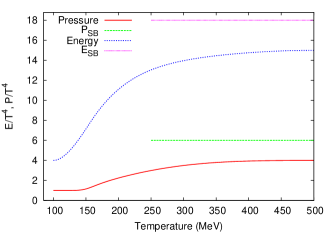
In order to construct the EoS for a crossover transition we considered the most recent results of lattice QCD simulations obtained by the Wuppertal-Budapest collaboration (see Ref. Borsanyi2010 ), with , i.e. two light (up and down) and one heavy (strange) quarks. To adapt such EoS to the conditions prevailing at the QCD epoch in the early universe we added the contribution of a gas of non-interacting neutrinos (), muons, electrons, photons and their antiparticles, all them described by an EoS of the form with . As showed in Ref. Borsanyi2010 the addition of the charm or heavier quarks doesn’t introduce any substantial modification in the temperature regime relevant for this work. Such data generate smooth curves for several observables which are typical of a crossover transition. In Fig. 1 we show the behavior of the pressure and the energy density for a large range of temperatures as well as the Stefan-Boltzmann limit.
III Numerical Approach
The hydrodynamic equations presented in Eq. (2) can be recast as a hyperbolic system of first-order, flux-conservative equations of the form Font2002 :
| (3) |
where in the laboratory frame the state vector contains the conserved variables written in terms of primitive variables
| (4) |
and the flux vector is given by
| (5) |
with being the Lorentz factor. The elements of the flux matrix are the mass flux , the momentum flux plus pressure force , and the energy flux plus pressure work . Note that the flux vector is written in terms of the conserved variables of the state vector.
The conservation laws written in the form of a Eq. (3) allow to solve the problem numerically through a wealth of methods. In the present work we shall employ a High-Resolution Shock-Capturing scheme (HRSC) which is recognized as a very efficient scheme for dealing with complex flows specially when discontinuities are present (see e.g. Anton2006 and references therein). These methods use the equations in conservative form together with approximate or exact Riemann solvers to calculate the numerical fluxes between neighboring computational cells. This fact guarantees the capture of all discontinuities (e.g., shock waves) which naturally appear in spatial solutions of the non-linear hyperbolic equations and allows high accuracy in regions where the fluid flow is smooth. These schemes depend on the spectral decomposition of the Jacobian matrix which has a complete set of linearly independent eigenvectors (characteristic fields) , and corresponding eigenvalues (characteristic velocities) such that
| (6) |
In the one dimensional case and in a flat Universe the eigenvalues are given by Font2000 ; Banyuls1997
| (7) |
that correspond to the slopes of three families of curves, known as material () and acoustic () waves. The relativistic speed of sound for an EoS in which the pressure is a function of and is given by
where , , is the entropy per particle, and the total energy density.
The linearly independent eigenvectors corresponding to each eigenvalue are
| (8) | |||
| (9) |
Our numerical code is based on the Godunov method Godunov1959 and the numerical fluxes are obtained using the well known Riemann solver of Roe Pike1984 ; Toro2009 :
| (10) |
which has the advantage that can be straightforwardly implemented for an arbitrary EoS. The numerical fluxes and are computed using respectively the primitive variables to the left and right of the interface. Both and are computed by Eqs. (7 9) using the following weighted quantities:
| (11) | |||||
| (12) | |||||
| (13) |
The quantities represent the jumps of the characteristic variables across each characteristic field and are obtained from the inversion of:
| (14) |
In order to avoid spurious oscillations we use a monotone upstream centered scheme for conservation laws (MUSCL), with a standard “minmod” sloper limit Font:2002kb for the reconstruction of the cell centered quantities before the computation of the numerical fluxes. The integration in time is performed by using a third order strong-stability-preserving Runge-Kutta scheme with five stages Gottlieb2008 .
IV Gravitational Radiation Spectra
To determine the gravitational signal emitted by the motion of the primordial fluid, we adopt the formalism presented in Ref. Weinberg1972 , which has also been used in Refs. (Kosowsky1993, ; Kamionkowski1994, , among others). All the information needed to calculate the gravitational wave spectrum is contained in purely spatial components of the stress-energy tensor that, in our case, is obtained from the hydrodynamic simulation. Following this treatment, the gravitational energy radiated per solid angle is given by
| (15) |
where
| (16) |
is know as projection tensor. The stress-energy tensor is obtained by a fast Fourier transform (FFT) defined as Weinberg1972 ; Kamionkowski1994
| (17) |
Since our hydrodynamic simulations are performed in one spatial dimension, our problem is axially symmetric about the axis. Thus, we can take without loss of generality Kosowsky1992
| (18) |
Therefore, the projector tensor reads:
| (19a) | ||||
| (19b) | ||||
| (19c) | ||||
| (19d) | ||||
Finally, the total energy per unit frequency interval emitted as gravitational radiation is given by (c.f. Kosowsky1992 )
| (20) |
where , and are the Fourier transforms of
| (21) |
| (22) |
Integrating Eq. (20) over the solid angle, the same expression as in Eq. (23) of Ref. Kosowsky1993 is obtained 222In the present work we focus on the hydrodynamic evolution of a small portion of the primordial fluid with a size of 100 m. Since we perform 1D simulations, our computational domain can be viewed as a cube where the fluid moves only along the z-axis. Thus, the gravitational emission of the domain is not isotropic but depends on the angle with respect to the z-axis, forming an antenna pattern like the ones presented in Kosowsky1992 . This angular dependence is an artifact of the 1D simulation, but, fortunately, we are interested in the energy density of the gravitational waves, which depends on the angle-averaged emission of the domain. Anyway, differences are to be expected with respect to 2D and 3D simulations, which will be addressed in future work.
| (23) |
In order to compare our results with eLISA/NGO, we describe the spectrum in terms of a characteristic amplitude of the stochastic background defined as Maggiore1999
| (24) |
where , being the Hubble constant, and is the energy density of the gravitational waves,
| (25) |
being the critical density. Finally, we have to consider the redshift suffered by the waves in their way to the present Universe Maggiore1999 :
| (26) | |||||
| (27) |
where the subscript corresponds to present values and the subscript to the values at the epoch of the transition.
V Turbulence in the crossover QCD transition
Since we are considering a crossover transition at the QCD epoch, we don’t expect large perturbations near the critical temperature as it would be the case for a first order transition. Thus, we assume that fluctuations present at the QCD epoch were generated by some event in the previous history of the Universe, e.g. at the electroweak phase transition that occurred at . Hence, one may consider that the size of the larger fluctuations at the QCD era are of the order of the size of the horizon at the electroweak era; i.e. we have . In other words, the injection of energy happens at the electroweak scale ( m) or at an even smaller scale related to inflation 333According to Schwarz1997 , Seto and Yokoyama Seto2003 , and Boyle and Steinhardt Boyle2005 the spectrum of gravitational waves produced at inflation is modified by a variety of post-inflationary physical effects, in particular, deviations from the standard equation of state () during the radiation era. For example, large drops in the number of relativistic particles during a QCD transition would lead to steps in the spectrum of gravitational waves Schwarz1997 . The study of such reprocessing of the inflationary background during the QCD epoch is out of the scope of the present paper. However, it is necessary to properly understand and disentangle the all post-inflationary effects Boyle2005 , like the here studied QCD transition, in order to optimally extract the inflationary information in the stochastic gravitational wave background., cosmic strings, etc. Binetruy2012 . This fluctuations are conjectured to survive until the beginning of the QCD phase transition due to the extremely large Reynolds number of the primordial fluid large_Re .
In turbulent fluids, we usually have a large stirring length scale at which turbulent eddies are injected in the fluid. As said above, we are assuming that large fluctuations occur at (or before) the electroweak era and therefore, the stirring scale is . As the larger eddies break down to smaller ones, there is a cascade of kinetic energy from large to small scales. This cascade effect will stop at a small damping length scale determined by the viscosity of the fluid. Roughly, the damping scale is determined by a Reynolds number close to 1, . Thus we can estimate the order of magnitude of the damping scale as , where is the kinematic viscosity of the fluid and its typical velocity.
The shear viscosity of matter at the QCD epoch can be derived from heavy-ion collision experiments at the Relativistic Heavy-Ion Collider (RHIC) and the Large Hadron Collider (LHC). In fact, these experiments show that the quark-gluon plasma at temperatures behaves as a nearly perfect quark-gluon liquid with a viscosity per entropy density in the range Song2011 ; Heinz2012 , i.e. approaching the Kovtun-Policastro-Son-Starinets lower bound Kovtun2005 . Since the baryon chemical potential and temperature of the RHIC/LHC fluid are not exceedingly different to what it is expected at the early Universe we may assume that the primordial fluid at the QCD transition behaves as a perfect fluid as well. According to this, we would have which is 14 orders of magnitude smaller than the size of the cell in our numerical simulations, which is . However, the contribution of leptons and photons to the viscosity may be significant. In fact, theoretical estimations Ahonen1999 of the viscosity of the quark-gluon plasma (QGP) in the early Universe give values that are roughly one order of magnitude larger than the experimental values obtained at RHIC and LHC. The viscosity may be up to three orders of magnitude larger if electrons, muons and photons are included in the QGP, and even eight orders of magnitude larger if neutrinos are considered Ahonen1999 . In spite of this, the viscosity is still very small and the Reynolds number very large, as generally considered in the literature. Actually, when the most viscous composition is considered, the damping length scale is m, which is still orders of magnitude smaller than the size of the cell in our numerical simulations. Therefore, the use of the ideal hydrodynamic equations presented in Sec. II is fully justified.
Up to now, most works studying the QCD transition have considered that the distribution of turbulent kinetic energy density has a stationary spectrum consistent with the Kolmogorov phenomenology Kamionkowski1994 ; Kosowsky2002 ; Megevand2008 , i.e. scaling as or variations of this Dolgov2002 ; Kahniashvili2010 . This spectrum is very frequent in astrophysical environments, like the interplanetary, interstellar or intergalactic medium, which have a significant viscosity and a constant injection of energy at the large scales (induced e.g. by solar flares, supernovae, etc.). This energy is transferred to small scales through a cascading effect until , where kinetic energy is dissipated into heat due to the fluid viscosity, resulting a spectrum with a negative slope. In the cosmological case, the assumption of a Kolmogorov-like spectrum may be acceptable when there is a continuous injection of energy, as in the case of a first order phase transition, for which bubble collisions introduce a continuous stirring. However, this stirring is not present in a crossover transition, and therefore the assumption of a Kolmogorov spectrum is unjustified. Moreover, since the viscosity of the primordial fluid is tiny, dissipation at small scales does not occur at the same rate as the energy is accumulated by cascading. Therefore, a very different turbulent spectrum is to be expected.


VI Results
We have carried out relativistic one-dimensional hydrodynamic simulations for an ideal non-viscous fluid employing the fluid equations and EoS of Sec. II. We consider a computational domain with a length of 100 m, with 16.384 spatial cells () and evolve the system for times larger than . The choice of these intervals is related to the band of the spectrum of gravitational waves that we want to obtain from the numerical simulations, i.e. Hz according to the eLISA’s sensitivity curve (see below). We consider reflective boundary conditions, so that we may see the Universe as a set of various contiguous domains of 100 m. Due to choice of the boundary conditions, disturbances are reflected several times during the simulation, representing the fluid interaction with neighboring regions having similar profiles. In agreement with the above discussion, turbulence is included only through inhomogeneities in the initial condition. We have considered three different kinds of random initial profiles: (a) random temperature inhomogeneities in a fluid at rest, (b) random velocity fluctuations within a fluid with an initial uniform temperature, and (c) random temperature and velocity fluctuations. Since the size of possible disturbances at the time of the transition is unknown we consider fluctuations of maximum amplitude around MeV and/or in the initial profile. Our goal is to determine the smallest fluctuation amplitude that would be detected by eLISA, considering the motion of the fluid induced by the initial condition as a source of gravitational radiation. The hydrodynamic simulations provide the tensor from which we obtain through a FFT. This allows the calculation of the spectrum of the gravitational radiation emitted by the fluid through Eq. (23).
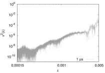
In Fig. 2 we consider random temperature inhomogeneities with a maximum amplitude of in a fluid that is initially at rest. The initial temperature profile (top panel) presents peaks and valleys of different sizes. As the fluid evolves, these temperature gradients induce the motion of the fluid, temperature inhomogeneities are smoothed (see central panel of Fig. 2), and the fluid develops a turbulent motion with velocities up to . As discussed before, there is a cascading that transports kinetic energy to the smallest scales where there is no dissipation due to the absence of viscosity. This behavior is apparent in the bottom panel of Fig. 2, which shows that a large amount of kinetic energy is accumulated at the smallest scales (large ) at the end of the simulation. We performed similar simulations with random temperature inhomogeneities with a maximum amplitude of and . The hydrodynamic evolution is not shown here because the behavior is qualitatively the same.
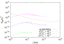
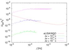
In Fig. 3 we can see a comparison between the gravitational wave spectra arising from the three initial temperature gradients considered here. In the case with the signal would be detected by eLISA for a wide range of frequencies. For the simulation with the signal is entirely below but not too far from the eLISA’s threshold. In fact, we can show that the signal for fluctuations of about is partially overlapping the eLISA’s sensitivity curve. Fluctuations with don’t lead to enough motion in the fluid to emit a significant amount of gravitational radiation.


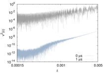


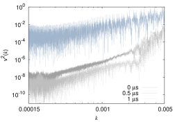
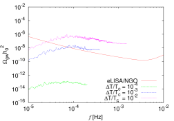
We also considered an initial condition with constant temperature MeV and a random velocity distribution. For an initial maximum amplitude of (see top panel of Fig. 4) the turbulent motion creates temperature gradients of the order of which at the end of simulation fall to about with maximum velocities roughly the half of the initial (see central panel of Fig. 4). On the bottom panel of Fig. 4, we show the initial and final velocity spectra, which present the same behavior as in the previous simulations, confirming the expectation that the spectra must be very different to the Kolmogorov power law. For maximum initial velocities of , the induced temperature gradients are an order of magnitude larger than in the previous case and the strong motion of the fluid leads to a large amount of gravitational radiation (Fig. 5). Notice that the spectrum with is almost overlapping the eLISA sensitivity curve for frequencies larger that Hz as in the simulation with initial condition , . In spite of these initial conditions being very different, the system evolves in both cases to similar temperature and velocity profiles in a timescale considerably smaller than the total time of the simulation. In fact, simulations with concomitant velocity and temperature gradients in the initial condition give essentially the same results as before, i.e. a progressive homogenization of both the temperature and velocity profiles, an energy cascade to the smaller scales, and a gravitational wave spectrum with a peak around Hz (see Figs. 68). This peak in the spectrum is due to an exponential decay of the fluid velocity. Actually, we verified that with s for most values of the wave number , showing that most of the fluid motion happens within this time interval. Since gravitational wave emission is associated with the level of turbulent motion in the fluid, we expect a maximum in the spectrum at a frequency , which from Eq. (26) turns out to be Hz; i.e. consistent with the maximum in the spectra of Figs. 3, 5 and 8.
VII Summary and Conclusions
In this paper, we have studied the evolution of primordial turbulence in the universe at the QCD epoch using a state-of-the-art equation of state derived from lattice QCD simulations Borsanyi2010 . Since the transition is a crossover, we don’t expect large perturbations near the critical temperature as it would be the case for a first order transition. Thus, we assume that temperature and velocity fluctuations were generated by some event in the previous history of the Universe (e.g. a first order transition at the electroweak scale or at an even smaller scale related to inflation, cosmic strings, etc.) with typical sizes smaller than the size of the horizon at the electroweak era, . Due to the extremely large Reynolds number of the primordial fluid we consider that these inhomogeneities are able to survive until the QCD epoch.
The primordial fluid at the QCD epoch is assumed to be non-viscous, based on the fact that the viscosity per entropy density of the quark gluon plasma obtained from heavy-ion collision experiments at the RHIC and the LHC is extremely small, more specifically, in the range at temperatures Song2011 ; Heinz2012 . For the hydrodynamic simulations, we considered a one dimensional computational domain with a length of 100 m divided in cells, injected random temperature and velocity fluctuations in the initial conditions, and evolved the system for times larger than . Our results show that the velocity spectrum is very different from the Kolmogorov power law considered in most studies of primordial turbulence that focus on first order transitions. This is due to the fact that there is no continuous injection of energy in the system and the viscosity of the fluid is negligible. Thus, as kinetic energy cascades from the larger to the smaller scales, a large amount of kinetic energy is accumulated at the smallest scales due to the lack of dissipation (see bottom panels of Figs. 2 and 4, and Fig. 7).
We have obtained the spectrum of the gravitational radiation emitted by the motion of the fluid for different initial profiles that include random temperature and velocity fluctuations of different maximum amplitudes. We find that if typical fluctuations have an amplitude and/or , they would be detected by eLISA at frequencies larger than Hz.
Acknowledgements.
V. R. C. Mourão Roque acknowledges the financial support received from UFABC and CAPES. G. Lugones acknowledges the financial support received from FAPESP.References
- (1) S. Borsányi et al., JHEP 09, 073 (2010).
- (2) M. Cheng et al., Phys. Rev. D 81, 054504 (2010).
- (3) S. Borsányi et al., Journal of High Energy Physics 11, 077 (2010); Y. Aoki et al., Nature 443, 675 (2006).
- (4) P. Binétruy, A. Bohé, C. Caprini, and J. F. Dufaux, JCAP 06, 27 (2012).
- (5) K. Ishidoshiro et al., Phys. Rev. Lett. 106, 161101 (2011).
- (6) E. Witten, Phys. Rev. D 30, 272 (1984).
- (7) J. H. Applegate and C. J. Hogan, Phys. Rev. D 31, 3037 (1985).
- (8) A. G. Polnarev, Soviet Astron. 29, 607 (1985).
- (9) A. Rotti and T. Souradeep, Phys. Rev. Lett. 109, 221301 (2012).
- (10) J. C. Miller and L. Rezzolla, Phys. Rev. D 51, 4017 (1995); M. S. Turner e F. Wilczek. Phys. Rev. Lett. 65, 3080, (1990).
- (11) A. Kosowsky and M. S. Turner, Phys. Rev. D 47, 4372 (1993).
- (12) M. Kamionkowski, A. Kosowsky, and M. S. Turner, Phys. Rev. D 49, 2837 (1994).
- (13) A. Kosowsky, A. Mack, and T. Kahniashvili, Phys. Rev. D 66, 024030 (2002).
- (14) A. D. Dolgov, D. Grasso, and A. Nicolis, Phys. Rev. D 66, 103505 (2002).
- (15) A. Nicolis Class. Quant. Grav. 21, L27, (2004).
- (16) T. Kahniashvili, G. Gogoberidze, and B. Ratra, Phys. Rev. Lett. 95, 151301 (2005)
- (17) T. Kahniashvili, A. Kosowsky, G. Gogoberidze, and Y. Maravin, Phys. Rev. D 78, 043003 (2008).
- (18) C. Grojean and G. Servant, Phys. Rev. D 75, 043507 (2007)
- (19) G. Gogoberidze, T. Kahniashvili, and A. Kosowsky, Phys. Rev. D 76, 083002 (2007).
- (20) C. Caprini, R. Durrer, and R. Sturani, Phys. Rev. D 74, 127501 (2006).
- (21) T. Kahniashvili, L. Kisslinger, and T. Stevens, Phys. Rev. D 81, 23004 (2010).
- (22) P. Amaro-Seoane et al., Class. Quantum Grav. 29, 124016 (2012).
- (23) S. Weinberg, Gravitation and Cosmology: Principles and Applications of the General Theory of Relativity (Wiley, New York, 1972).
- (24) P. Fragile and P. Aninos, Phys. Rev. D 67, 103010 (2003).
- (25) J. A. Font et al., Phys. Rev. D 65, 084024 (2002).
- (26) L. Antón et al., Astrophys. J. 637, 296 (2006).
- (27) J. A. Font, M. Miller, W. M. Suen, and M. Tobias, Phys, Rev. D 61, 044011 (2000).
- (28) F. Banyuls, J. A. Font, J. M. Ibáñez, J. M. Martí, and J. A. Miralles, Astrophys. J. 476, 221 (1997).
- (29) S. K. Godunov, Math. Sbornik 47, 271 (1959).
- (30) E. F. Toro, Riemann Solvers and Numerical Methods for Fluid Dynamics: A Practical Introduction., 3rd ed. (Springer-Verlag, 2009).
- (31) P. L. Roe and J. Pike, “Computing methods in applied science and engineering”, in Computing Methods in Applied Science and Engineering (INRIA North-Holland, 1984).
- (32) J. Font et al., Phys. Rev. D 64, 084024 (2002).
- (33) S. Gottlieb, D. I. Ketcheson, and C.-W. Shu, J. Sci. Comput. 38, 251–289 (2008).
- (34) A. Kosowsky, M. S. Turner, and R. Watkins, Phys. Rev. D 45, 4514 (1992).
- (35) M. Maggiore, Phys. Rept. 331, 283 (2000).
- (36) G. Baym et al., Phys. Rev. Lett. 64, 1867 (1990); H. Heiselberg, Phys. Rev. D 49, 4739 (1994); G. Baym, D. Bodeker, and L. McLerran, Phys. Rev. D 53, 662 (1996); J. Ahonen, Phys. Rev. D 59, 023004 (1998).
- (37) H. Song, S. Bass, U. Heinz, T. Hirano, and C. Shen, Phys. Rev. Lett. 106, 192301 (2011).
- (38) U. W. Heinz, C. Shen, and H. Song, AIP Conf. Proc. 1441, 766-770 (2012).
- (39) P.K. Kovtun, D.T. Son, A.O. Starinets, Phys. Rev. Lett. 94, 111601 (2005).
- (40) J. Ahonen, Phys Rev D D59, 023004 (1999).
- (41) A. Mégevand, Phys. Rev. D 78, 084003 (2008).
- (42) T. Kahniashvili, A. Brandenburg, A. G. Tevzadze, and B. Ratra, Phys. Rev. D 81, 123002 (2010).
- (43) A.R. Kerstein, J. Fluid Mech. 392, 277 (1999).
- (44) A. R. Kerstein, T. D. Dreeben, Phys. Fluids 12, 418 (2000), A. R. Kerstein, Comput. Phys. Commun. 148, 1 (2002), R. C. Schmidt, A. R. Kerstein, S. Wunsch, V. Nilsen, J. Comput. Phys. 186, 317 (2003), S. Wunsch, A. R. Kerstein, J. Fluid Mech. 528, 173 (2005), H. Shihn, P.E. DesJardin, Int. J. Heat Mass Transfer 50, 1314 (2007).
- (45) T. Echekki, A.R. Kerstein, T.D. Dreeben, Combust. Flame 125, 1083 (2001), B. Ranganath, T. Echekki, Prog. Comput. Fluid Dynam. 6, 409 (2006), B. Ranganath, T. Echekki, Combust. Flame 154, 23 (2008), D. O. Lignell and D. S. Rappleye, Combust. Flame 159, 2930 (2012).
- (46) D. J. Schwarz, Mod. Phys. Lett. A13, 2771 (1998)
- (47) N. Seto and J. Yokoyama, J. Phys. Soc. Jap. 72, 3082 (2003).
- (48) L. A. Boyle and P. J. Steinhardt, Phys. Rev. D77, 063504 (2008).