A Catalog of Ultra-compact High Velocity Clouds from the ALFALFA Survey: Local Group Galaxy Candidates?

Abstract

We present a catalog of 59 ultra-compact high velocity clouds (UCHVCs) extracted from the 40%-complete ALFALFA HI-line survey. The ALFALFA UCHVCs have median flux densities of 1.34 Jy km s^-1, median angular diameters of 10^′, and median velocity widths of 23 km s^-1. We show that the full UCHVC population cannot easily be associated with known populations of high velocity clouds. Of the 59 clouds presented here, only 11 are also present in the compact cloud catalog extracted from the commensal GALFA-HI survey, demonstrating the utility of this separate dataset and analysis. Based on their sky distribution and observed properties, we infer that the ALFALFA UCHVCs are consistent with the hypothesis that they may be very low mass galaxies within the Local Volume. In that case, most of their baryons would be in the form of gas, and because of their low stellar content, they remain unidentified by extant optical surveys. At distances of $\sim$1 Mpc, the UCHVCs have neutral hydrogen (HI) masses of $\sim 10^{5}-10^{6}$ $M_{\odot}$, HI diameters of $\sim 2-3$ kpc, and indicative dynamical masses within the HI extent of $\sim 10^{7}-10^{8}$ $M_{\odot}$, similar to the Local Group ultra-faint dwarf Leo T. The recent ALFALFA discovery of the star-forming, metal-poor, low mass galaxy Leo P demonstrates that this hypothesis is true in at least one case. In the case of the individual UCHVCs presented here, confirmation of their extragalactic nature will require further work, such as the identification of an optical counterpart to constrain their distance.

1. Introduction

One of the well-known problems in the study of galaxies is the paucity of observed low mass galaxies compared to the numbers of them predicted by dark matter simulations. In the context of the Local Group (LG), this is known as the “missing satellites” problem (Klypin et al., 1999; Moore et al., 1999). This discrepancy between simulations and observations is also seen in the difference between the slope predicted for the low mass end of the dark matter halo mass function and the observed slopes of the luminosity function (Blanton et al., 2005), neutral hydrogen (HI) mass function (Martin et al., 2010), and velocity width function (Papastergis et al., 2011).

During the last decade, much progress has been made in understanding these discrepancies. The general mismatch between simulations and observations is widely understood to be the result of astrophysical processes impacting the observable baryons. While simulations are improving at including baryonic physics, many of the relevant processes occur on subgrid scales, leaving many details and specifics as active areas of research. However, the gross effects of baryon physics are understood. Hoeft & Gottlöber (2010) show that simply including the effects of reionization in simulations roughly accounts for the majority of the discrepancy, with baryon content dropping drastically below a critical dark matter halo mass of $\sim 10^{10}$ $M_{\odot}$, near the threshold where galaxy counts are observed to drop dramatically. The true situation is more complicated; star formation feedback processes are more efficient in massive galaxies but more effective in low mass galaxies so that the baryon content is most depressed at the high and low mass ends of the mass spectrum (Hoeft & Gottlöber, 2010; Guo et al., 2010; Evoli et al., 2011; Reyes et al., 2012; Papastergis et al., 2012).

In this context, we distinguish a galaxy from a dark matter halo by the presence of observable baryons. While the general mismatch between predicted dark matter halos and visible galaxies is understood, the specifics are not well known. Is there a minimum galaxy mass that can form? Are there galaxies with a single stellar population? How does star formation proceed in the lowest mass systems? Which processes are dominant in the baryon loss from the lowest mass systems? One way to answer these questions is to observe the lowest mass galaxies that are most impacted by these issues.

The advent of wide-field optical surveys increased the number of known Milky Way (MW) satellites with the discovery of the ultra-faint dwarf galaxies (UFDs). The UFDs have luminosities from $10^{2}-10^{5}$ $L_{\odot}$, half-light radii from 20-350 pc and $M/L$ ratios of 100 to over 1000, total masses within the baryon extent of $10^{6}-10^{7}$ $M_{\odot}$, generally old stellar populations, and are located at distances of tens to a few hundred kpc from the MW (Martin et al., 2008; Simon & Geha, 2007). The name ultra-faint is well earned – the total luminosities of these objects are comparable to those of globular clusters, but they are clearly galaxies as their kinematics indicate they are dark matter dominated (Simon & Geha, 2007). The discovery of UFDs is exciting and opens many possibilities into addressing the fundamental questions of how marginal galaxies form; however there is one problem – nearly all the UFDs are located within the virial radius of the MW. Bovill & Ricotti (2011) predict based on simulations that the vast majority of UFDs have been modified by tides; this is supported by observational evidence of tidal disruption (Simon & Geha, 2007; Muñoz et al., 2010; Sand et al., 2012). This makes it nearly impossible to determine which of the UFD properties, such as sizes and kinematics, are primeval and which are result of environmental influence from interaction with the MW. Bovill & Ricotti (2011) do predict the existence of $\sim$100 fossil galaxies with luminosities less than $10^{6}$ $L_{\odot}$ that have remained isolated from the Milky Way at distances of 400 kpc to 1 Mpc.

One UFD is of particular note. Leo T lies at distance of 420 kpc, safely outside the virial radius of the MW and was, until recently, the only gas-rich UFD discovered. Leo T is a star-forming galaxy with a HI mass of 2.8 $\times$ $10^{5}$ $M_{\odot}$, an HI diameter of 600 pc, an indicative dynamical mass within the HI extent of $\sim$3.3$\times$ $10^{6}$ $M_{\odot}$, a total-mass-to-light ratio within the HI extent of 56, and a stellar mass of $\sim$1.2 $\times$ $10^{5}$ $M_{\odot}$ (Ryan-Weber et al., 2008). Given its gas content and distance, Leo T likely represents an unperturbed UFD, allowing environmental effects to be disentangled from the evolution of the lowest-mass galaxies. Indeed, Rocha et al. (2012) argue that Leo T is on its first infall to the Milky Way. Leo T is on the edge of detectability for SDSS; were it located further away, its stellar population would not have been detected (Kravtsov, 2010). UFDs with properties similar to Leo T but located further from the MW or with fainter stellar populations would have been overlooked in the automated searches of SDSS. However, the HI content of Leo T would be detectable in a sensitive, wide area HI survey, raising the possibility that more isolated, gas-rich UFDs await discovery.

Exploiting the huge collecting area of the Arecibo 305m telescope and the mapping capability of its 7 beam receiver (ALFA), the Arecibo Legacy Fast ALFA (ALFALFA) HI line survey is the first blind HI survey capable of addressing this issue in a robust way. Surveying over 7000 square degrees of sky, ALFALFA has the sensitivity to detect $10^{5}$ $M_{\odot}$  of HI with a linewidth of 20 km s^-1  at 1 Mpc. In fact, the recent discovery of Leo P from ALFALFA survey data shows that galaxies similar to Leo T in the Local Volume may be identified via their 21cm line emission. (Giovanelli et al., 2013; Rhode et al., 2013; Skillman et al., 2013). Leo P was discovered during the normal course of identifying HI detections within the ALFALFA survey when it was noticed that one ultra-compact high velocity cloud (UCHVC) could be associated with an irregular, lumpy light distribution in the SDSS images (Giovanelli et al., 2013). Follow-up optical observations resolved a stellar population and a single HII region, confirming that the UCHVC is in fact a low mass galaxy, Leo P (Rhode et al., 2013). We stress that Leo P was confirmed to be a galaxy because its young, blue stellar population was barely visible in the SDSS images; without recent star formation, the underlying older population of Leo P would not have been visible at all in the SDSS images. Leo P was discovered by its HI signature, and its existence strongly argues that other very low mass and (nearly) starless objects are included among the ALFALFA UCHVCs.

We (Giovanelli et al., 2010, hereafter G10) originally discussed a set of ultra-compact high velocity clouds (UCHVCs) that were consistent with being gas-bearing low mass dark matter halos at $\sim$1 Mpc; we referred to this interpretation of the UCHVCs as the minihalo hypothesis. In this paper, we expand on this work and present a catalog of UCHVCs for the current 40% ALFALFA data release, termed $\alpha$.40 (Haynes et al., 2011). We offer further detail on the minihalo hypothesis for this class of objects, drawing special attention to the properties of Leo T and Leo P. We note that the idea that LG dwellers could be identified by their HI content was first proposed by Braun & Burton (1999) and Blitz et al. (1999). The UCHVCs presented here overcome objections raised against the initial sample of clouds proposed to represent gas-rich galaxies in the LG.

In Section 2 we discuss the $\alpha$.40 data and selection of UCHVCs. In Section 3 we present the UCHVC catalog and overview the observed properties of the UCHVCs. In Section 4 we examine the UCHVC population in the context of the known high velocity cloud (HVC) populations, and in Section 5 we present evidence supporting the LG origin and minihalo hypothesis for the UCHVCs. In Section 6, we summarize our findings.

2. Data

The sources presented here are found within the footprint of the $\alpha$.40 release of the ALFALFA survey (Haynes et al., 2011) but correspond to a separate analysis of the same spectral data cubes. We briefly describe the ALFALFA survey below, with an emphasis on its relevance to UCHVCs, followed by a description of how the UCHVCs are identified and measured. The ALFALFA sky is divided into two regions, termed the “spring” and “fall” as a result of our nighttime observing in the Northern Hemisphere. The “spring” ALFALFA sky covers a range of $7.5h-16.5h$ in RA; the “fall” sky is $22h-3h$ in RA. The $\alpha$.40 footprint covers approximately 2800 square degrees and includes the declination ranges 4^∘-16^∘ and 24^∘-28^∘  in the spring, and 14^∘-16^∘ and 24^∘-32^∘ in the fall. We note here that Leo P is located at +18^∘ and is not in the $\alpha$.40 footprint, and hence is not included in the UCHVC sample. The footprint of the $\alpha$.40 survey can be seen in Figure 1; the top panel is the spring sky and the bottom panel is the fall sky. The relative sizes of the panels indicate the different RA coverage of the separate survey areas. The open diamonds in the figure show the general HVC population of the $\alpha$.40 survey and the filled symbols are the UCHVCs of this work with the gray scale (color in the online version) indicating the velocities of the clouds. The fall sky shows a prevalence of HVCs; in comparison, the spring sky is relatively clean, making this a better location to look for low mass gas-bearing dark matter halos.

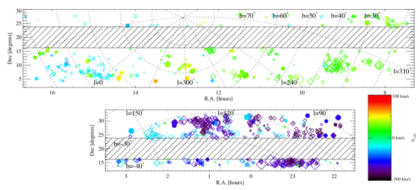
Figure 1.— UCHVCs (filled circles) plotted in R.A.-Dec. coordinates; gray scale (color in the online version) corresponds to the velocity of the cloud. The solid squares are the most-isolated subsample of UCHVCs (see Section 2.4). The open diamonds are the $\alpha$.40 HVCs shown for reference. The size of the symbols is proportional to the angular sizes of the HVCs in all cases but not to scale. The top panel is the spring R.A. region; the bottom panel the fall R.A. region. The hashed region corresponds to declination ranges not covered by $\alpha$.40. The fall sky shows prevalent HVC structure while the spring sky is relatively clear of HVCs.

2.1. The ALFALFA Survey

ALFALFA is an extragalactic spectral line survey making use of the Arecibo 305m telescope. The survey maps 7000 square degrees of sky in the HI 21cm line, covering the spectral range between 1335 and 1435 MHz (roughly -2500 km s^-1 to 17500 km s^-1 for the HI line), with a spectral resolution of 25 kHz, or $\sim 5.5$ km s^-1 (at $z=0$). ALFALFA is designed to outperform previous blind HI surveys. With an angular resolution of $\sim 3^{\prime}.5$, ALFALFA can resolve structures 1/4 the angular size possible with the HI Parkes All Sky Survey (HIPASS; Meyer et al., 2004) and 1/9 that possible with the Leiden Dwingeloo Survey (LDS; Hartmann & Burton, 1997). Its flux density sensitivity is nearly one order of magnitude higher than that of HIPASS and more than two orders of magnitude better than that of the LDS. ALFALFA can detect a $\sim 5\times 10^{4}$ $M_{\odot}$ cloud of 20 km s^-1 linewidth at a distance of 1 Mpc. A full description of the observational mode of ALFALFA is given in Giovanelli et al. (2007), while the definition and goals of the survey are described in Giovanelli et al. (2005). Only a summary of the observational details is given here.

ALFALFA surveys the sky using a seven–feed multi-beam receiver in “drift” mode: the telescope is normally parked along the local meridian and 14 tracks (7 feeds, 2 polarizations each) of spectral data of 4096 channels – each acquired continuously and recorded at a 1 Hz rate as the sky drifts by. All regions of the sky are visited twice with the two visits typically a few months apart in time. Upon completion of data taking of a region of the sky, data cubes of 2^∘.4 $\times$ 2^∘.4 in spatial coordinates are produced and sampled over a regular grid of 1^′ spacing in R.A. and Dec. After Hanning smoothing to 11 km s^-1 resolution, the rms noise per channel of the data is typically 2 to 2.5 mJy per beam. In general, sources are extracted from the data cubes through a 2–step process. An automated signal identification algorithm is first run over each data cube, producing a preliminary source catalog (Saintonge, 2007). Then each source in the catalog is visually inspected and remeasured. The measurement tool fits ellipses to contours of constant flux density level and delivers a source position, given by the center of the ellipse encircling half of the total flux density of the source, source sizes (as the major and minor axes of said ellipse), flux density, velocity and linewidth.

2.2. Source Identification

As mentioned above, the standard source identification and measurement in ALFALFA uses the algorithm developed by Saintonge (2007) to identify sources and is then followed by measurement of the source by hand. Briefly, the identification algorithm is a one-dimensional matched filtering scheme. The spectrum in each pixel of an ALFALFA grid is matched to a series of Hermite polynomial templates. The detection of a galaxy requires the detection of spectra of similar velocity widths with a high significance in 5 or more contiguous pixels.

Figure 2.— The distribution of HI angular diameters and full width half maximum of the HI line ($W_{50}$) for the UCHVCs (filled histograms), $\alpha$.40 sources classified as reliable extragalactic detections (unfilled histograms), and $\alpha$.40 HVCs (hashed histograms). The UCHVCs and HVCs occupy a small range of narrow velocity widths. The UCHVCs are spatially large compared to the extragalactic detections but generally small compared to the $\alpha$.40 HVCs.

In comparison with the extragalactic sources identified in the $\alpha$.40 catalog, the UCHVCs are typically spatially extended and have narrow velocity widths. This is illustrated in Figure 2 where the distribution of HI angular diameters and velocity widths are plotted for the $\alpha$.40 extragalactic sources, $\alpha$.40 HVCs and the UCHVCs of this work. The UCHVCs are spatially extended compared to the extragalactic sources but generally small compared to the full HVC population of the $\alpha$.40 survey. The minimum velocity width used in the templates of the Saintonge (2007) identification algorithm is 30 km s^-1, the typical maximum width of the UCHVCs. For this reason, a special source identification algorithm was developed for the UCHVCs in addition to the standard ALFALFA pipeline. This method is based on the philosophy of Saintonge (2007), but with three main differences: a limited velocity range, three-dimensional matched filtering, and the use of gaussian templates. Only a limited velocity range of the ALFALFA data set, -500 < $v_{\odot}$ < 1000 km s^-1, is selected as this is the expected velocity range for objects within the Local Volume. Because only a limited velocity range is examined, it is reasonable to perform a full three-dimensional matched filtering, matching both the spectrum of the source and the spatial position and size simultaneously. Gaussian templates are used to describe both the spatial extent and the velocity profile of the UCHVCs. The templates range from a spatial full width half maximum (FWHM) size of 4^′ to 12^′  in steps of 2^′ and the spectral line FWHM ranges from 10 km s^-1 to 40 km s^-1  in steps of 6 km s^-1. The lower bound of the spatial templates is set by the beam size of Arecibo. The upper size bound is near the median size value of the UCHVCs and represents our emphasis on detecting ultra-compact clouds. UCHVCs can be larger in size than 12^′  and the matched filtering of the 12^′ template to a UCHVC with HI diameter greater than 12^′ is robust. A velocity FWHM of 10 km s^-1  represents the narrowest source that can be spectroscopically resolved in the ALFALFA data. The warm neutral medium is thought to be the dominant phase of the ISM in minihalos (e.g. Sternberg et al., 2002); for a reasonable range of temperatures ($6000-10000$ K) for the warm neutral medium in the UCHVCs, thermal broadening results in linewidths of $\sim 16-21$ km s^-1. Thus for a cloud of 40 km s^-1 linewidth, we would expect the large scale motion to be $\sim$34 km s^-1 for the warmest clouds, after subtracting the thermal broadening contribution in quadrature. For a typical size of 10^′ at an indicative distance of 1 Mpc, the dynamical mass based on this unbroadened linewidth is $\sim 10^{8}$ $M_{\odot}$. This is a reasonable upper limit to the dynamical mass we may expect to be traced out for a more massive dark matter halo of $\lesssim 10^{10}$ $M_{\odot}$, and matches the dynamical mass traced by the baryon extent of the presumably more massive SHIELD galaxies (Cannon et al., 2011).

Many of the UCHVCs are missed by the standard identification algorithm. Since the ALFALFA pipeline also involves visual inspection of the dataset, most of these sources are identified by eye and included in the $\alpha$.40 catalog as HVC detections. The specialized UCHVC identification algorithm does find sources that are missed by the standard ALFALFA pipeline; of the 59  UCHVCs identified here (listed in Table 1), 5  sources are not included in the $\alpha$.40 catalog. Three of these are in the spring sky and two in the fall sky. Figure 3 shows the measured properties of all the UCHVCs compared to the 5 sources not included in the $\alpha$.40 catalog. The additional sources tend to have low integrated flux densities and narrow linewidths ($W_{50}$). While they have a range of HI diameters, they are not the most compact clouds. Most strikingly, the UCHVCs not included in the $\alpha$.40 catalog are the sources with the lowest average column densities, suggesting that these sources are the tip of the iceberg for further clouds to be detected.

Figure 3.— The measured properties for the full sample of UCHVCs (unfilled histograms) compared to the UCHVCs found specifically by the separate analysis presented in this work (hashed histograms). Generally, the new UCHVCs have narrow velocity widths and low fluxes. They also have low $\bar{N}_{HI}$ values.

2.3. Criteria for UCHVC Identification

To be included as a UCHVC in the catalog, a source must have $|v_{LSR}|$ > 120 km s^-1, have a HI major axis less than 30^′ in size, and have a S/N $\geq$ 8 to ensure reliability. The $v_{LSR}$ limit is imposed to focus on a class of clouds that are well separated from Galactic emission and that could trace dark matter halos within the LG. Some dark matter halos would be expected to have $|$$v_{LSR}$$|$ < 120 km s^-1 (Leo T, for example) but disentangling their emission from Galactic hydrogen is challenging and left to future work. The 30^′ size limit corresponds to a physical size of 2 kpc at a distance of 250 kpc. The distance of 250 kpc is a reasonable minimum distance for an unperturbed object at the edge of the MW; Grcevich & Putman (2009) find that LG dwarf galaxies with neutral gas content 270 kpc away from either the MW or M31. We would not expect to detect low mass galaxies with large gas reservoirs nearer to the MW due to interaction with the hot Galactic corona (Fukugita & Peebles, 2006). Note that Leo T has an HI diameter of 0.6 kpc, and Leo P has an HI diameter of 1.2 kpc. The models of Sternberg et al. (2002) for gas in dark matter minihalos predict HI diameters up to 3 kpc with diameters less than 2 kpc a more common outcome. It should be noted that most UCHVCs are smaller than this criterion, with only six clouds having average HI diameters larger than 16^′ (see Figure 3). The S/N limit of 8 ensures reliability. This limit is higher than the general reliability limit of the ALFALFA survey data due to the different nature of the UCHVCs, including the strong potential for radio frequency interference (RFI) to masquerade as narrow-line sources. Confirmation observations of low S/N sources are ongoing, and in future work we will examine the reliability and completeness of the ALFALFA UCHVC catalog.

2.4. Isolation

Given the abundance of HVC structures in the sky, the most important criterion for determining if a cloud is a good minihalo candidate is its isolation. Most of the known HVC structure is associated with Galactic processes, including accretion onto the Milky Way; when considering clouds that could represent gas associated with dark matter halos, we wish to find objects distinct from existing HVC structures. In order to be considered a UCHVC, visual inspection must ensure that the cloud does not appear to be associated with a larger HI structure.

Table 1ALFALFA UCHVCs in the $\alpha$40 Survey

Source	AGC	R.A.+Dec.	cz⊙ $V_{lsr}$ $V_{gsr}$ $V_{LG}$	$W_{50}(\epsilon_{w})$	$a\times b$	$S_{21}$	S/N	$N_{3}$	$N_{10}$	Notes
		J2000	km s-1	km s-1	′	Jy km s-1
HVC111.65-30.53-124	103417	000554.3+312014	-128 -124   55  139	21 ( 8)	27 $\times$ 15	2.31	12	0	9	g, O
HVC123.11-33.67-176	102992	005206.2+291204	-177 -176  -19    61	21 ( 3)	24 $\times$ 10	1.28	9	0	5	g, O
HVC123.74-33.47-289	102994	005431.6+292402	-290 -289 -133  -52	21 ( 1)	6 $\times$  5	0.67	15	0	13	g, O
HVC126.85-46.66-310	749141	010237.8+160752	-308 -310 -186 -112	23 ( 6)	10 $\times$  8	0.81	9	1	21	g, O
HVC131.90-46.50-276	114574	011703.4+155548	-273 -276 -160  -88	27 ( 4)	10 $\times$  6	0.71	9	1	22	g, O
HVC137.90-31.73-327	114116	014952.1+292600	-325 -327 -199 -124	34 ( 8)	29 $\times$ 16	3.93	13	1	9	g, O
HVC138.39-32.71-320	114117	015031.4+282259	-317 -320 -194 -119	22 ( 2)	19 $\times$ 13	4.41	30	1	7	g, O, S12
HVC154.00-29.03-141	122836	025229.7+262630	-135 -141  -55     8	27 ( 3)	29 $\times$ 15	6.90	31	0	15	g, O
HVC205.28+18.70+150	174540	074559.9+145837	162  150   59   42	23 ( 4)	10 $\times$ 6	2.06	28	0	2	g, S12, O
HVC196.50+24.42+146	174763	075527.1+244143	156  146   88   79	20 ( 2)	16 $\times$ 11	2.80	20	3	11	g, S12, O
HVC196.09+24.74+166	174764	075614.8+250900	175  166  110  101	24 ( 6)	10 $\times$  5	0.66	9	3	10	p, O
HVC198.48+31.09+165	189054	082546.7+251128	173  165  104   90	26 ( 1)	19 $\times$ 13	1.77	13	0	8	g, O
HVC204.88+44.86+147	198511	093013.2+241217	152  147   80   53	15 ( 1)	8 $\times$  6	0.73	14	0	0	g, S12, O
HVC234.33+51.28+143	208315	102701.1+084708	148  143   29  -22	20 ( 2)	15 $\times$ 10	4.96	35	0	16	g, S12
HVC250.16+57.45+139	219214	110929.8+052601	142  139   25  -32	20 ( 5)	7 $\times$  4	0.56	10	0	9	g, G10, S12
HVC252.98+60.17+142	219274	112119.6+062132	143  142   35  -22	27 ( 5)	28 $\times$ 15	8.55	37	1	10	g, S12
HVC253.04+61.98+148	219276	112624.8+073915	149  148   47   -8	36 ( 1)	14 $\times$ 12	2.06	14	1	11	g
HVC255.76+61.49+181	219278	112855.6+062529	182  181   77   19	18 ( 2)	11 $\times$  6	0.90	13	0	7	g, S12
HVC256.34+61.37+166	219279	112928.6+060923	167  166   61     3	24 ( 1)	12 $\times$ 11	1.49	14	2	11	g
HVC245.26+69.53+217	215417	114008.1+150644	216  217  146   97	17 ( 4)	10 $\times$  9	0.70	9	0	1	g, G10
HVC277.25+65.14-140	227977	120920.0+042330	-142 -140 -234 -294	23 ( 1)	7 $\times$  4	0.46	8	0	1	g, G10
HVC274.68+74.70-123	226067	122154.7+132810	-128 -123 -182 -232	54 (13)	5 $\times$  4	0.92	11	0	0	p, G10
HVC290.19+70.86+204	226165	123440.2+082408	200  204  135   80	21 ( 1)	10 $\times$  6	0.90	11	1	15	g
HVC292.94+70.42+159	229344	123758.5+074849	154  159   89   34	15 ( 4)	17 $\times$ 14	1.67	13	0	18	g
HVC295.19+72.63+225	226170	124204.6+095405	220  225  164  112	28 ( 7)	14 $\times$ 12	1.17	10	3	16	p, G10
HVC298.95+68.17+270	227987	124529.8+052023	265  270  196  139	26 ( 1)	16 $\times$  9	5.58	44	0	4	g, G10
HVC324.03+75.51+135	233763	131242.3+133046	127  135  102   56	29 ( 1)	7 $\times$  5	0.94	18	1	12	g
HVC320.95+72.32+185	233830	131321.5+101257	177  185  141   92	23 ( 9)	21 $\times$ 16	1.70	9	0	15	g, G10
HVC330.13+73.07+132	233831	132241.6+115231	124  132  100   53	16 ( 1)	6 $\times$  3	0.63	11	0	11	g, G10
HVC326.91+65.25+316	238713	133043.8+041338	308  316  264  210	26 ( 4)	12 $\times$ 10	1.25	11	0	0	p, G10
HVC 28.09+71.86-144	249393	141058.1+241204	-157 -144 -111 -136	43 ( 6)	15 $\times$  9	1.12	8	0	0	g, O
HVC353.41+61.07+257	249323	141948.6+071115	246  257  244  201	20 ( 4)	13 $\times$  9	1.34	13	3	4	g, G10
HVC351.17+58.56+214	249282	142321.2+043437	203  214  196  151	40 ( 8)	7 $\times$  5	1.45	17	0	4	p, G10, S12
HVC352.45+59.06+263	249283	142357.7+052340	252  263  248  203	32 ( 9)	16 $\times$ 11	1.11	8	3	4	g, G10
HVC356.81+58.51+148	249326	143158.8+063520	136  148  141  100	38 (11)	6 $\times$  5	0.70	10	0	1	p
HVC 5.58+52.07+163	258459	150441.3+061259	149  163  176  141	24 ( 8)	11 $\times$ 10	1.33	13	0	4	g
HVC 13.59+54.52+169	258237	150723.0+113256	155  169  200  170	23 ( 3)	10 $\times$  5	1.34	17	1	3	g
HVC 13.60+54.23+179	258241	150824.4+112422	164  179  210  180	17 ( 1)	15 $\times$  7	0.99	11	1	4	g
HVC 13.63+53.78+222	258242	151000.6+111127	207  222  253  224	21 ( 2)	9 $\times$  6	0.71	9	0	1	g, G10
HVC 26.11+45.88+163	257994	155354.0+144148	146  163  232  217	23 ( 3)	12 $\times$  7	2.04	22	2	8	g
HVC 26.01+45.52+161	257956	155507.5+142929	144  161  230  215	25 ( 6)	8 $\times$  6	1.54	14	2	8	g
HVC 29.55+43.88+175	268067	160529.4+160912	158  175  255  244	37 (11)	10 $\times$  6	1.91	20	2	6	g, G10
HVC 28.07+43.42+150	268069	160532.6+145920	132  150  227  214	29 ( 4)	10 $\times$  5	1.15	11	0	10	g, G10
HVC 28.47+43.13+177	268070	160707.0+150831	160  177  255  243	20 ( 3)	17 $\times$  9	1.48	11	2	6	g, G10
HVC 28.03+41.54+127	268071	161236.8+141226	109  127  206  194	62 (15)	12 $\times$  7	2.67	18	1	8	g
HVC 28.66+40.38+125	268072	161745.3+141036	108  125  208  197	42 ( 5)	16 $\times$  9	3.17	21	3	7	g
HVC 19.13+35.24-123	268213	162235.7+050848	-139 -123  -63  -81	17 ( 1)	12 $\times$ 10	2.83	22	0	7	g, G10, S12
HVC 27.86+38.25+124	268074	162443.4+124412	107  124  207  197	23 ( 4)	11 $\times$  9	1.28	13	2	4	g
HVC 84.01-17.95-311	310851	215406.2+311249	-324 -311  -98  -21	21 ( 4)	26 $\times$ 14	2.60	17	0	5	g
HVC 82.91-20.46-426	310865	215802.9+283735	-439 -426 -217 -140	22 ( 1)	12 $\times$  6	0.99	10	0	17	g, S12
HVC 80.69-23.84-334	321318	220100.7+244404	-345 -334 -131 -55	23 ( 1)	18 $\times$  9	1.47	13	0	5	g
HVC 86.18-21.32-277	321455	221121.8+295402	-288 -277  -68    10	17 ( 1)	13 $\times$  7	1.76	15	0	5	g, O
HVC 82.91-25.55-291	321320	221238.6+244311	-302 -291  -90  -13	24 ( 2)	15 $\times$  6	1.31	13	0	7	g, O
HVC 84.61-26.89-330	321351	222134.4+243638	-341 -330 -130  -53	21 ( 4)	13 $\times$ 11	1.03	9	0	8	g, O
HVC 92.53-23.02-311	321457	223823.4+315257	-321 -311 -104  -23	28 ( 2)	19 $\times$  9	1.68	12	0	5	g, O
HVC 87.35-39.78-454	334256	230056.4+152014	-461 -454 -282 -206	26 ( 4)	11 $\times$  8	1.57	16	0	1	g, O
HVC 88.15-39.37-445	334257	230211.3+160048	-452 -445 -271 -195	22 (11)	12 $\times$  4	0.68	10	0	4	g, O
HVC108.98-31.85-328	333613	235658.8+293235	-333 -328 -147  -64	19 ( 2)	13 $\times$  5	0.55	8	1	19	g, O
HVC109.07-31.59-324	333494	235702.1+294846	-329 -324 -143  -60	17 ( 5)	12 $\times$  7	1.80	23	1	19	g, O

Our second isolation criterion is that the UCHVCs must be well separated from previously known HVC complexes. We compare the UCHVCs to the updated catalog of Wakker & van Woerden (1991, B. Wakker, private communication 2012; hereafter WvW). The WvW catalog includes 617 clouds, of which 393 are classified as belonging to 20 large complexes; the other clouds are classified into populations based on their spatial coordinates and velocity. For defining isolation, we only consider the WvW clouds which are part of a larger complex. The distance of a UCHVC from another cloud in degrees can be quantified via:

$$D=\sqrt{\theta^{2}+(f\delta v)^{2}},$$ (1)

where $\theta$ is the angular separation in degrees, $\delta v$ is the velocity difference in km s^-1 between two clouds, and $f$ is a conversion factor that parameterizes the significance we ascribe to the angular separation between two clouds versus their difference in velocity in determining whether they are associated with each other. Following Saul et al. (2012) and Peek et al. (2008), we adopt $f=0.5$^∘/km s^-1 as the weighting for the velocity separation for large scale HVC structure. Figure 4 illustrates our determination of the isolation criterion for deciding if the UCHVCs are separated from the WvW complexes. The isolation criterion was determined by comparing the separation of clouds within WvW complexes to the separation of LG galaxies from the nearest WvW cloud in a complex. The x-axis shows the distance to the nearest WvW cloud in a complex and the y-axis shows the fraction of objects whose closest neighbor is at that distance or closer (cumulative fraction). Ninety percent of WvW clouds in complexes are closer than 15^∘ to their nearest neighbor in the complex; more than eighty percent of LG galaxies are located further than 15^∘ from the nearest WvW cloud in a complex. Hence we determine to use this value as our cutoff, shown by the dot-dash line in Figure 4. We note that is a more generous criteria than that of Saul et al. (2012) and Peek et al. (2008) who adopt $D=25$^∘ as an isolation criterion; in Section 4.1 we examine this intermediate distance and determine it does not substantially affect our catalog.

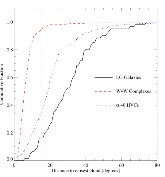
Figure 4.— The relative isolation of LG galaxies and $\alpha$.40 HVCs from the large HVC complexes of WvW. The x-axis is the distance to the closest WvW cloud in a complex calculated using Equation 1. The y-axis shows the fraction of objects that have their nearest neighbor at that distance or nearer. The separation of WvW clouds within complexes from each other is shown by the dashed line (red in the online version). The isolation of the LG galaxies is shown by the solid line (black in the online version), and the $\alpha$.40 HVCs are shown for reference with the dotted line (blue in the online version). The dot-dash line indicates our chosen isolation criterion of $D=15$^∘. The majority of clouds in complexes are within 15^∘ of their nearest neighbor, although there is a smaller tail extending to 25^∘. The majority of LG galaxies are located further than 15^∘ from a cloud in a complex, making this a good isolation criterion. This isolation criterion removes $\sim$30% of the $\alpha$.40 HVCs from consideration as UCHVCs, but further isolation criteria are clearly necessary.

In addition, we institute a third isolation criterion based on HVC structure uncovered by ALFALFA. This structure is generally much smaller than previously known HVC structure; as can be seen in Figure 2 most $\alpha$.40 HVCs are less than one degree in size while the sizes of the HVCs in the WvW catalog are several to tens of degrees. For this reason, we use $f=0.2$^∘/km s^-1 in Equation 1 when calculating isolation from HVC structure within the ALFALFA survey. The top panel of Figure 5 shows the final isolation criterion for UCHVCs and compares the UCHVCs to LG galaxies and the general HVC detections within the $\alpha$.40 survey. We require that the UCHVCs have no more than three neighbors within $D=3$^∘. This is a generous criterion as the LG galaxies have at most one neighbor within this distance. We wish to include all potential minihalo candidates and inspection indicates that allowing three neighbors includes all the sources that would be classified by eye as isolated. In the bottom panel of Figure 5 we explore the differences between the spring and fall populations of the UCHVCs. The fall sky appears to show more isolation on this scale with the UCHVCs having either one or no neighbors; in fact, this is a result of the prominent HVC structure in the fall sky. Clouds in the fall sky are either part of a larger structure or have no (or one) neighbors within $D=3$^∘. Comparing to the general $\alpha$.40 HVC population shows the prevalence of HVC structure in the fall sky with the fall HVCs generally having more neighbors than the spring HVCs.

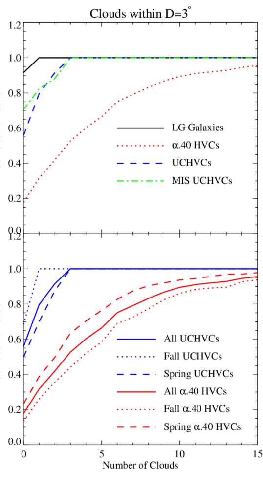
Figure 5.— The x-axis is the number of $\alpha$.40 HVCs within $D=3$^∘, where the distance is calculated from Equation 1 with $f=0.2$ ^∘/km s^-1, and the y-axis is the fraction of UCHVCs with that number of neighbors or fewer. The top panel shows the relative isolation of LG galaxies (solid line, black in online version), UCHVCs (dashed line, blue in online version), MIS UCHVCs (dot-dash line, green in online version), and general $\alpha$.40 HVCs (dotted line, red in online version). The LG galaxies have no more than one $\alpha$.40 HVC within $D=3$^∘; the criteria for the UCHVCs is slightly relaxed to not more than 3 neighbors. The $\alpha$.40 HVCs are shown for reference; a majority of the $\alpha$.40 HVCs fail this isolation criteria. In the bottom panel, we compare the spring (dashed line) and fall populations (dotted line) of the UCHVCs (blue in the online version), with the $\alpha$.40 HVCs shown for references (red in the online version).

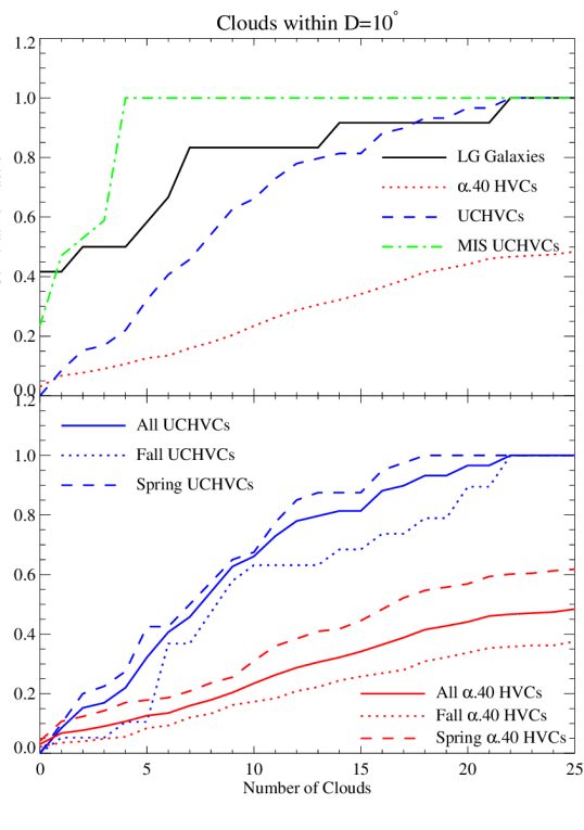
Figure 6.— The x-axis is the number of $\alpha$.40 HVCs within $D=10$^∘, where the distance is calculated from Equation 1 with $f=0.2$ ^∘/km s^-1, and the y-axis is the fraction of UCHVCs with that number of neighbors or fewer. The top panel shows the relative isolation at this larger distance scale of LG galaxies (solid line, black in online version), UCHVCs (dashed line, blue in online version), MIS UCHVCs (dot-dash line, green in online version), and general $\alpha$.40 HVCs (dotted line, red in online version). At this distance scale, the UCHVCs and LG galaxies have similar behavior. We define a most-isolated subsample (MIS) of UCHVCs which are still isolated with no more than 3 neighbors on this larger scale. The MIS UCHVCs are even more isolated than the LG galaxies on this larger scale. In the bottom panel, we compare the spring (dashed line) and fall populations (dotted line) of the UCHVCs (blue in the online version), with the $\alpha$.40 HVCs shown for references (red in the online version).

We note that with this criterion, only clouds with central velocities within 15 km s^-1 of the UCHVC can be considered as neighbors. Given that the median velocity width of the UCHVCS is 23 km s^-1, there is a possibility that this isolation criterion could leave our sources kinematically confused. Our first isolation criterion accounts for this through the examination of the UCHVCs for association with other clouds. In order to verify this, we examine the effect of changing the velocity weighting factor to $f=0.05$^∘/km s^-1. This expands the velocity selection to 60 km s^-1, almost three times the median FWHM of the clouds. We examine the number of clouds within 3^∘ of the UCHVCs using this different value of $f$ and find that the UCHVCs still have very few neighbors with this modified distance estimate. In fact, seventy-five percent of the UCHVCs still meet the criterion of three or fewer neighbors even when the expanded velocity space is considered. We examined the nine UCHVCs with more than five neighbors and note that three of them may possibly be kinematically associated with larger structure; we mark these UCHVCs in Table 1.

HVC structure often exists on scales much larger than 3^∘; while the UCHVCs are examined for obvious connection to larger structure and excluded in that case, we still wish to define a more isolated subsample. As the best subsample to represent HI sources associated with minihalo candidates, we define a “most-isolated” subsample (MIS) of UCHVCs with no more than than 4 neighbors within $D=10$^∘. The top panel of Figure 6 shows the number of neighboring clouds within $D=10$^∘ for the UCHVCs, the MIS UCHVCs, LG galaxies and $\alpha$.40 HVCs. On this large scale, the MIS UCHVCs are generally more isolated than even the LG galaxies. We do note that the $\alpha$.40 footprint means that we are not generally probing to a full 10^∘ in all directions around a given cloud; increasing coverage of the ALFALFA survey may change the classification of a cloud in the future. In fact, two sources in the fall $\delta=+15$^∘ strip meet the MIS criteria but we exclude them from this subsample as determining isolation out to 10^∘ for sources in an isolated 2^∘ wide strip is problematic. We will revisit these two specific sources and the classification of the MIS UCHVCs in general with increased ALFALFA coverage in future work. In the bottom panel of Figure 6, we again examine the difference between the fall and spring population. Here, the prominent HVC structure in the fall sky is apparent with many of the fall UCHVCs having a large number of neighbors out to a distance of 10^∘. There is also a strong difference evident between the UCHVC and $\alpha$.40 HVC population with over half of the $\alpha$.40 HVCs having more than 20 neighbors at $D=10$^∘; this indicates the utility of our first isolation criterion of inspecting sources for connection to large scale structure.

3. Catalog

3.1. Presentation of Catalog

In Table 1 we present the UCHVCs; there are 59 sources total: 40 in the spring $\alpha$.40 sky and 19 in the fall sky. Of the 59 UCHVCs, 17 are identified as being in the most-isolated subsample, all of which are in the spring sky. The spring sky samples the outer regions of the LG where the expected density for dark matter halos may be lower but the environment is safer for gas-bearing minihalos than near the MW or M31. The fall sky samples the LG near M31 and includes the presence of a large amount of HVC structure, including the Magellanic Stream (see Section 4.1 for a further discussion). We indicate those UCHVCs that are part of the original sample of UCHVCs discussed by G10 with a G10 in the notes column and those UCHVCs that lie outside the area considered by G10 with an ‘O’. Figure 7 shows maps of all the UCHVCs with contours in units of column density of HI ($N_{HI}$ in atoms cm^-2), representing the sum total of HI content along the line of sight; these plots represent the data from which all the parameters listed in Table 1 are derived. The minimum contour level is given in the figure and subsequent contour levels increase by factors of $\sqrt{2}$. We plot the contours in values of $N_{HI}$ to demonstrate that the peak column density value is higher than the average value calculated later (see Section 3.4). However, we emphasize, that since these clouds are barely resolved by the Arecibo beam, the column density contour values are only approximate and the average values are more robust; to accurately map the distribution of HI will require synthesis observations that provide a smaller beam. Column density values can be derived from the brightness temperature via:

$$N_{HI}=1.823\times 10^{18}\int T_{B}\,dv\,\,[{\rm cm}^{-2}].$$ (2)

In simple cases, the brightness temperature is related to the flux density at 21cm via:

$$T_{B}=\frac{606}{\theta^{2}}S$$ (3)

where $\theta$ is the (circular) beam in arcseconds and $S$ the flux in mJy/beam.

Figure 7.— Maps of the HI column density of the UCHVCs derived from ALFALFA spectral grids. Starred figures indicate membership in the most-isolated subsample. Ellipses (red in the online version) represent the measured half-power level. The 3^′.5 circular beam is shown in the lower left corner of all plots. The lowest contour level is listed in the upper left corner of each plot; subsequent contours increase by factors of $\sqrt{2}$.

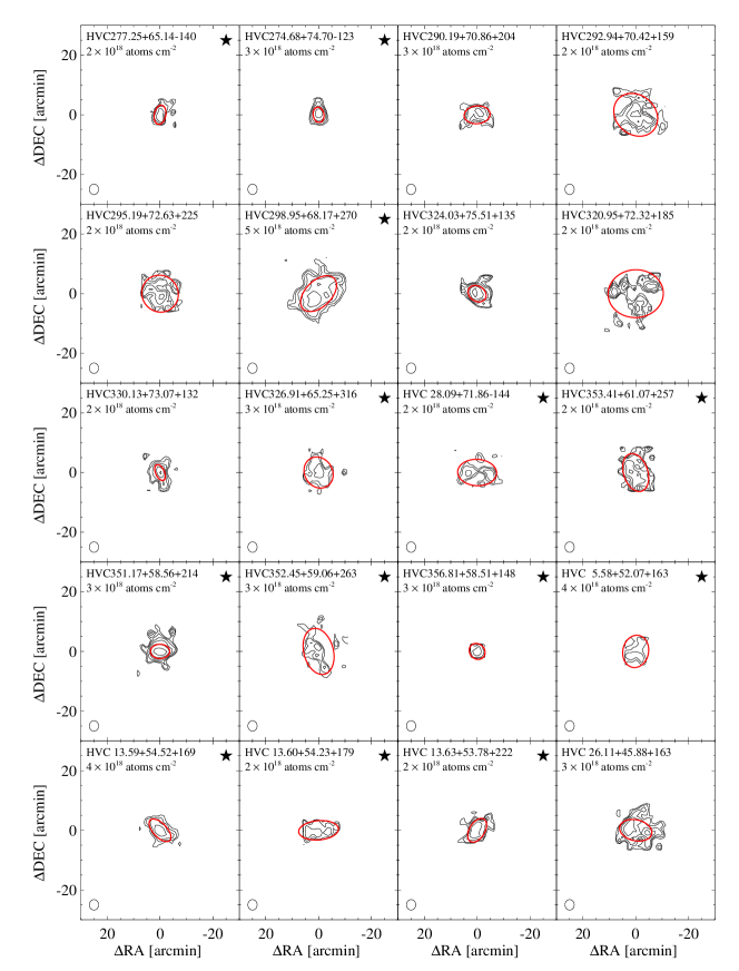
Figure 7.— Continued

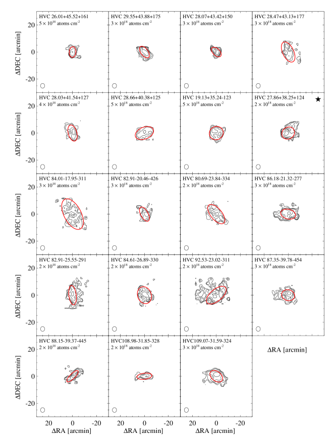
Figure 7.— Continued

The columns of the tables are as follows:

• Col. 1: Source name, in the traditional form for HVCs, obtained from the galactic coordinates at the nominal cloud center and the $v_{LSR}$ of the cloud, e.g. HVC111.65-30.53-124 has $l=$111.65^∘, $b=$-30.53^∘, and $v_{LSR}$= -124 km s^-1.

• Col. 2: Identification number in the Arecibo General Catalog (AGC), an internal database maintained by MH and RG, included to ease cross–reference with our archival system and the $\alpha$.40 catalog.

• Col. 3: Equatorial coordinates of the centroid, epoch J2000. Typical errors are less than 1^′.

• Col. 4: Sequentially, we list heliocentric velocity, velocity in the local standard of rest frame (LSR; assumed solar motion of 20 km s^-1 towards $l=57^{\circ}$, $b=25^{\circ}$), velocity in the Galactic standard of rest frame (GSR; $V_{gsr}=V_{lsr}+225\sin l\cos b$, with both velocities in km s^-1), and the velocity with respect to the LG reference frame from Karachentsev & Makarov (1996).

• Col. 5: HI line full width at half maximum ($W_{50}$), with estimated measurement error in brackets. The notes column indicates the method of measurement: a gaussian fit or linear single peaks fit to the sides of the profile.

• Col. 6: Estimate of the cloud major and minor diameters, in arcminutes. Sizes are measured at approximately the level encircling half the total flux density. In many cases, the outer contours are more elongated than indicated by the ratio $a\times b$. The half-power ellipses are also shown in the HI column density contour plots in Figure 7.

• Col. 7: Flux density integral ($S_{21}$), in Jy km s^-1.

• Col. 8: Signal–to-noise ratio (S/N) of the line, defined as

  $$S/N=(\frac{1000S_{21}}{W_{50}})\frac{w_{smo}^{1/2}}{\sigma_{rms}},$$ (4)

  where $S_{21}$ is the integrated flux density in Jy km s^-1, as listed in Column 7; the ratio 1000$S_{21}$/$W_{50}$ is the mean flux density across the feature in mJy; $w_{smo}$ is $W_{50}$/(2 $\times$ 10), a smoothing width, and $\sigma_{rms}$ is the rms noise figure across the spectrum measured in mJy. More details on the S/N calculation are available in Haynes et al. (2011).

• Col. 9: The number of $\alpha$.40 HVC neighbors within $D=3$^∘ (for $f=0.2$^∘/km s^-1)

• Col. 10: The number of $\alpha$.40 HVC neighbors within $D=10$^∘ (for $f=0.2$^∘/km s^-1)

• Col. 11: Notes column. For each source there is either a ‘g’ or ‘p’ indicating the method used (gaussian or single peaks fit) to measure $W_{50}$. Sources considered by G10 are indicated with a ‘G10’ in the notes column. Sources that are outside the footprint considered in G10 are marked with a ‘O’. The UCHVCs that are also in the GALFA compact cloud catalog of Saul et al. (2012) are indicated with a ‘S12’.

3.2. Comparison to G10

For completeness, we include in Table 2 the UCHVCs that were considered by G10 but do not meet the stricter selection criteria used here. The clouds from G10 can fail any of the criteria: S/N, isolation or $v_{LSR}$ limits. The notes column indicates the reason a G10 cloud is not included here. The sources with S/N < 8 will be considered in future work when we extend the UCHVC catalog to lower S/N values after assessing reliability and completeness. In addition, we will extend the catalog to velocities including the Galactic hydrogen. It should be noted that the three sources that do not meet the isolation criteria only barely fail. Two sources have one and two more neighbors than allowed, respectively, and the third sources is excluded based on examination of large scale structure. These sources could still be good minihalo candidates.

Table 2UCHVCs from G10 that Fail UCHVC Criteria

Source	AGC	R.A.+ Dec.	cz⊙ $V_{lsr}$ $V_{gsr}$ $V_{LG}$	$W_{50}(\epsilon_{w})$	$a\times b$	$S_{21}$	S/N	$N_{3}$	$N_{10}$	Reason
		J2000	km s-1	km s-1	′	Jy km s-1
HVC244.51+53.41+160	208424	104850.1+050419	164  160   39  -18	19 ( 3)	16 $\times$ 12	1.03	7	0	9	S/N
HVC249.03+57.58+178	219213	110813.6+055725	179  176  64     5	19 ( 2)	12 $\times$  9	0.67	7	0	8	S/N
HVC247.19+70.29+247	215418	114418.2+150509	246  247  177  129	30 (10)	10 $\times$  8	0.54	7	0	1	S/N
HVC290.37+66.23-115	227983	123116.7+035044	-118 -114 -199 -259	20 (5)	6$\times$  4	0.44	9	0	3	Velocity
HVC298.30+72.91+185	226171	124557.2+100518	180  185  127   75	25 (3)	5 $\times$  4	0.57	9	5	21	Isolation
HVC299.62+67.65+326	227988	124619.1+044923	323  327  253  195	39 (13)	14 $\times$  7	0.76	6	0	0	S/N
HVC314.57+74.80+218	238626	130351.1+121223	211  218  176  127	36 (13)	5 $\times$  3	0.35	5	0	17	S/N
HVC 8.88+62.16+281	249538	143531.7+133126	269  282  298  264	18 ( 6)	4 $\times$  3	0.22	4	0	4	S/N
HVC 7.64+57.83-128	249248	144844.6+103510	-142 -128 -112 -147	22 (1)	25$\times$  5	1.83	16	0	42	Isolation
HVC 15.11+45.54-148	258474	154035.2+074334	-163 -147 -106 -132	27 (1)	7 $\times$  5	0.68	9	4	19	Isolation

3.3. Properties of the UCHVCs

Figure 8 shows the distribution of measured properties for the $\alpha$.40 UCHVCs and the most-isolated subsample: integrated flux density ($S_{21}$), average angular diameter ($\bar{a}=\sqrt{ab}$), velocity FWHM ($W_{50}$), and $v_{LSR}$. The UCHVCs have integrated flux densities of $\sim$0.66-8.55 Jy km s^-1, with the vast majority having integrated flux densities below 3.5 Jy km s^-1 and a median flux density of 1.34 Jy km s^-1. The singly hatched histograms are the UCHVCs in the most-isolated subsample. Note that the range of values for the MIS UCHVCs is similar to the larger UCHVC population, and the median values are essentially identical. The UCHVCs range in average diameter from essentially unresolved ($\sim$4^′) to just over 20^′ in size, with the vast majority less than 16^′ in size and a median size of 10^′. We note that there does appear to be a break in population based on size with UCHVCs clustered with HI diameters < 16^′ in size and a tail of a population extending to larger sizes (including objects with HI diameters > 30^′ not included in this work). We will explore this break in HI size in the HVC population in future work with a larger survey area. The $W_{50}$ values are centered around 15-30 km s^-1 with a few UCHVCs having widths extending up to 70 km s^-1; the median linewidth is 23 km s^-1. There are clouds whose velocities cluster near both $v_{LSR}$ $\pm$120 km s^-1, with a much stronger clustering of positive velocity clouds. However, when the MIS UCHVCs are considered, this clustering disappears. The vast majority of negative velocity clouds are also excluded from the MIS UCHVCs; the negative velocity clouds are predominantly in the fall sky, where large scale HI structure is much more prevalent, preventing the inclusion of any UCHVCs into the most-isolated subsample.

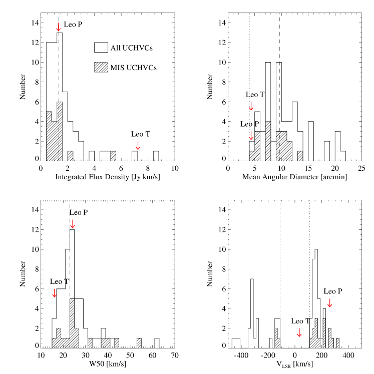
Figure 8.— Histograms of measured properties for the UCHVCs. Hashed histograms indicate the most-isolated subsample. The measured values for Leo T and Leo P from the ALFALFA data are indicated with arrows (red in the online version). The dashed lines are the median values of the UCHVCs; the most-isolated subsample has a slightly lower median flux density value and identical median values for the HI size and $W_{50}$. The dotted lines indicate observational boundaries. In the upper right panel, the dotted line indicates the smallest structure that can be resolved by Arecibo, and in the the bottom right panel the dotted lines indicate the velocity selection criterion.

3.4. Inferred Cloud Parameters

Given the observed properties of the UCHVCs, integrated flux density ($S_{21}$, Jy km s^-1), average angular diameter ($\bar{a}=\sqrt{ab}$, arcminutes) and velocity width ($W_{50}$, km s^-1), it is straightforward to derive some simple properties of the UCHVCs, modulo the unknown distance $d$ (in Mpc), with the assumption that the clouds are optically thin. Sequentially, below we derive the mean atomic density, mean column density, HI mass, indicative dynamical mass within the HI extent, and HI diameter.

$$\bar{n}_{HI}[\mathrm{atoms\ cm}^{-2}] = 0.74~{}S_{21}~{}\bar{a}^{-3}~{}d^{-1}\,\,\,\,{\rm cm}^{-3}$$ (5)

$$\bar{N}_{HI}[\mathrm{atoms\ cm}^{-2}] = 4.4\times 10^{20}~{}\bar{a}^{-2}~{}S_{21}\,\,\,\,{\rm cm}^{-2}$$ (6)

$$M_{HI}[M_{\odot}] = 2.356\times 10^{5}~{}S_{21}~{}d^{2}$$ (7)

$$M_{dyn}[M_{\odot}] = 6.2\times 10^{3}~{}\bar{a}~{}W_{50}^{2}~{}d$$ (8)

$$D_{HI}[\mathrm{kpc}] = 0.29~{}\bar{a}~{}d$$ (9)

Of these derived properties, $\bar{N}_{HI}$ is especially noteworthy as it does not depend on the distance. It should be noted that the column density values derived here are average values based on the global properties of the UCHVCs, in contrast to the approximation of spatially-resolved column density contours in Figure 7. Due to the large beam size of Arecibo, these values represent underestimates of the peak values of the clouds. We note that the dynamical mass is an indicative mass dynamical mass only. In addition to the uncertainty in the distance of the UCHVCs, the contribution to the linewidths of the UCHVCs from thermal broadening is unknown. For a range of reasonable temperatures, the thermal broadening can range from 16-21 km s^-1. For the clouds with the largest linewidths, the thermal broadening contribution (when accounted for in quadrature) may be negligible, while the narrowest clouds may be fully thermally supported. However, they could still have large-scale motions on the order of the thermal broadening, or less. For example, Leo P has a linewidth of 24 km s^-1 and a rotational velocity of 9 km s^-1, uncorrected for disk inclination (Giovanelli et al., 2013). To derive accurate dynamical masses will require higher resolution HI images in which evidence of large scale motions can be discerned (and, of course, distance information).

In Table 3, we summarize the inferred properties of the UCHVCs. The columns of the table are as follows:

• Col. 1 and 2: source id as in Table 1

• Col 3: HI diameter in kpc at $d=1$ Mpc (Eqn. 9)

• Col 4: log of the mean atomic HI density at $d=1$ Mpc, in cm^-3 (Eqn. 5)

• Col 5: log of the mean HI column density, in cm^-2 (Eqn. 6)

• Col 6: log of the HI mass at $d=1$ Mpc, in solar units (Eqn. 7)

• Col 7: log of the indicative dynamical mass within $D_{HI}$ at $d=1$ Mpc, in solar units (Eqn. 8)

Table 3Inferred Cloud Properties

Source	AGC	$D_{HI}$	$n_{HI}$	$\log~{}\bar{N}_{HI}$	$\log M_{HI}$	$\log M_{dyn}$
		kpc $d$	cm${}^{-3}d^{-1}$	cm-2	$M_{\odot}d^{2}$	$M_{\odot}d$
HVC111.65-30.53-124	103417	5.8	-3.68	18.40	5.74	7.74
HVC123.11-33.67-176	102992	4.6	-3.62	18.35	5.48	7.64
HVC123.74-33.47-289	102994	1.6	-2.54	18.98	5.20	7.18
HVC126.85-46.66-310	749141	2.7	-3.12	18.62	5.28	7.48
HVC131.90-46.50-276	114574	2.2	-2.95	18.72	5.22	7.54
HVC137.90-31.73-327	114116	6.2	-3.53	18.58	5.97	8.19
HVC138.39-32.71-320	114117	4.5	-3.07	18.90	6.02	7.67
HVC154.00-29.03-141	122836	6.0	-3.25	18.85	6.21	7.97
HVC205.28+18.70+150	174540	2.2	-2.46	19.19	5.69	7.40
HVC196.50+24.42+146	174763	3.8	-3.02	18.87	5.82	7.51
HVC196.09+24.74+166	174764	2.2	-2.94	18.71	5.19	7.43
HVC198.48+31.09+165	189054	4.6	-3.49	18.49	5.62	7.82
HVC204.88+44.86+147	198511	2.0	-2.81	18.81	5.24	6.99
HVC234.33+51.28+143	208315	3.6	-2.72	19.15	6.07	7.49
HVC250.16+57.45+139	219214	1.6	-2.58	18.93	5.12	7.13
HVC252.98+60.17+142	219274	5.8	-3.11	18.97	6.30	7.96
HVC253.04+61.98+148	219276	3.7	-3.14	18.74	5.69	8.01
HVC255.76+61.49+181	219278	2.4	-2.91	18.78	5.33	7.21
HVC256.34+61.37+166	219279	3.2	-3.10	18.72	5.55	7.60
HVC245.26+69.53+217	215417	2.8	-3.24	18.52	5.22	7.24
HVC277.25+65.14-140	227977	1.5	-2.64	18.86	5.03	7.24
HVC274.68+74.70-123	226067	1.3	-2.14	19.29	5.34	7.91
HVC290.19+70.86+204	226165	2.2	-2.83	18.83	5.33	7.32
HVC292.94+70.42+159	229344	4.4	-3.46	18.50	5.59	7.33
HVC295.19+72.63+225	226170	3.8	-3.41	18.48	5.44	7.80
HVC298.95+68.17+270	227987	3.5	-2.62	19.23	6.12	7.70
HVC324.03+75.51+135	233763	1.8	-2.51	19.05	5.35	7.50
HVC320.95+72.32+185	233830	5.3	-3.69	18.35	5.60	7.78
HVC330.13+73.07+132	233831	1.2	-2.23	19.17	5.17	6.83
HVC326.91+65.25+316	238713	3.1	-3.12	18.68	5.47	7.65
HVC 28.09+71.86-144	249393	3.3	-3.25	18.58	5.42	8.11
HVC353.41+61.07+257	249323	3.2	-3.12	18.69	5.50	7.43
HVC351.17+58.56+214	249282	1.7	-2.29	19.26	5.53	7.77
HVC352.45+59.06+263	249283	3.9	-3.46	18.44	5.42	7.92
HVC356.81+58.51+148	249326	1.6	-2.54	18.99	5.22	7.70
HVC 5.58+52.07+163	258459	3.0	-3.05	18.74	5.50	7.57
HVC 13.59+54.52+169	258237	2.0	-2.55	19.08	5.50	7.36
HVC 13.60+54.23+179	258241	2.9	-3.12	18.65	5.37	7.25
HVC 13.63+53.78+222	258242	2.1	-2.84	18.79	5.22	7.29
HVC 26.11+45.88+163	257994	2.7	-2.72	19.02	5.68	7.48
HVC 26.01+45.52+161	257956	1.9	-2.40	19.19	5.56	7.41
HVC 29.55+43.88+175	268067	2.2	-2.51	19.15	5.65	7.81
HVC 28.07+43.42+150	268069	2.1	-2.62	19.00	5.43	7.57
HVC 28.47+43.13+177	268070	3.5	-3.22	18.64	5.54	7.48
HVC 28.03+41.54+127	268071	2.7	-2.62	19.13	5.80	8.35
HVC 28.66+40.38+125	268072	3.4	-2.85	19.00	5.87	8.11
HVC 19.13+35.24-123	268213	3.1	-2.77	19.04	5.82	7.28
HVC 27.86+38.25+124	268074	2.8	-3.00	18.77	5.48	7.51
HVC 84.01-17.95-311	310851	5.4	-3.54	18.51	5.79	7.71
HVC 82.91-20.46-426	310865	2.4	-2.91	18.79	5.37	7.40
HVC 80.69-23.84-334	321318	3.7	-3.27	18.61	5.54	7.62
HVC 86.18-21.32-277	321455	2.8	-2.82	18.93	5.62	7.23
HVC 82.91-25.55-291	321320	2.7	-2.93	18.81	5.49	7.52
HVC 84.61-26.89-330	321351	3.5	-3.37	18.49	5.39	7.52
HVC 92.53-23.02-311	321457	3.8	-3.27	18.63	5.60	7.81
HVC 87.35-39.78-454	334256	2.7	-2.85	18.89	5.57	7.59
HVC 88.15-39.37-445	334257	2.0	-2.80	18.81	5.20	7.31
HVC108.98-31.85-328	333613	2.2	-3.02	18.63	5.11	7.23
HVC109.07-31.59-324	333494	2.7	-2.77	18.97	5.63	7.22

The HI masses, dynamical masses, mean atomic densities and mean column densities of the UCHVCs and the MIS UCHVCs are shown in Figure 9. At a distance of 1 Mpc, the HI masses are around $\sim 10^{5}-10^{6}$ $M_{\odot}$ and the dynamical masses are $\sim 10^{7}-10^{8}$ $M_{\odot}$. This would require the UCHVCs to have an ionized envelope of hydrogen or a substantial amount of dark matter in order to be self-gravitating. As discussed in Section 5, these median properties are a good match to the minihalo models of Sternberg et al. (2002). The median dynamical mass is $10^{7.5}\,d_{Mpc}$ $M_{\odot}$; this is close to the common mass scale of $\sim 10^{7}$$M_{\odot}$ for the UFDs of Strigari et al. (2008).

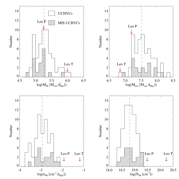
Figure 9.— The distribution of inferred properties for the UCHVCs. Shading and symbols are the same as in Figure 8. The most-isolated subsample has a slightly lower median mass than the full UCHVC sample; for other properties the median values are equivalent between the two samples. Leo T and Leo P are shown for comparison.

4. The UCHVCs as a Distinct Population

While the minihalo hypothesis is intriguing for the UCHVCs, we must carefully consider other possible explanations. In this section we examine the possibility of associating the UCHVCs with other cloud populations, including large HVC complexes, the Magellanic Stream, Galactic halo clouds, and the small cloud populations of the GALFA-HI survey.

4.1. The UCHVCs in the Context of Large HVC Complexes

The HVC sky contains many large extended structures composed of multiple clouds. We explicitly require the UCHVCs to be isolated from the known large scale HVC structure of the WvW catalog. However, our isolation criterion for separation from WvW complexes is slightly relaxed in order to avoid excluding potential minihalo candidates. As can be seen in Figure 4, the distance to the nearest cloud within a WvW complex can extend to $D=25$^∘. As we set our isolation criterion for UCHVCs to a separation of 15^∘ from WvW clouds in complexes, we wish here to consider the possible association of the UCHVCs with WvW complexes. In Table 4 we list the UCHVCs that are less than 25^∘ from a WvW complex. We note that only two UCHVCs in the fall sky (HVC86.18-21.32-277 and HVC87.35-39.78-454) are more than 25^∘ from a complex in the WvW catalog; the other fall HVCs not listed in Table 4 are separated by less than 25^∘ from clouds associated with the Magellanic Stream in the WvW catalog. Of the 40 spring UCHVCs, seven are potentially associated with known large complexes, the majority of those being with the WA complex. While a few of the UCHVCs may be associated with known large complexes, the vast majority are not, as defined by our isolation criterion.

Table 4UCHVCs within $D=25$^∘ of a WvW complex

Complex	UCHVC	Distance to closest cloud
		degrees
Complex G	HVC111.65-30.53-124	20.1
Complex H	HVC123.11-33.67-176	17.9
Complex ACVHV	HVC137.90-31.73-327	23.8
	HVC138.39-32.71-320	20.9
Complex ACHV	HVC154.00-29.03-141	15.1
Complex WC	HVC205.28+18.70+150	24.6
Complex WA	HVC234.33+51.28+143	16.3
	HVC250.16+57.45+139	19.3
	HVC252.98+60.17+142	21.9
	HVC253.04+61.98+148	24.6
	HVC256.34+61.37+166	24.7
Complex C	HVC 19.13+35.24-123	19.4

4.1.1 Magellanic Stream

The Magellanic Stream (MS) is an extended HI structure first noted by Dieter (1965) and first associated with the Magellanic Clouds by Mathewson et al. (1974). The MS is generally associated with the disruption of the Magellanic Clouds as they interact with the Milky Way, although the exact mechanisms responsible for the MS are an open area of research. The two main parts of the MS are the Leading Arm (LA), which consists of gas ahead of the Large Magellanic Cloud (LMC) and Small Magellanic Cloud (SMC) in their presumed orbits, and the tail, which consists of the trailing material. Recently, Nidever et al. (2010, hereafter N10) presented an extension of the Magellanic Stream (MS), bringing it to over a 200^∘ length in total. Given the extent of the MS, possible association with the MS must be considered when attempting to understand HVCs of any sort.

Figure 10.— The distribution of UCHVCs relative to the MS from N10. Coordinates are those of the MS-centric system from Nidever et al. (2008). The top panel is the spatial distribution of the MS; the x-axis is $L_{MS}$ and the y-axis $B_{MS}$. Shading (color coding in the online edition) of the MS indicates the column density, matching N10. The $\alpha$.40 footprint is shown in the top panel by the dashed lines. The red circles are the UCHVCs, the most-isolated subsample is indicated by the squares, and the white stars represent LG galaxies. The bottom panel is the total intensity of the Magellanic HI integrated along $B_{MS}$ (in units of K deg) and shows the kinematics of the MS.

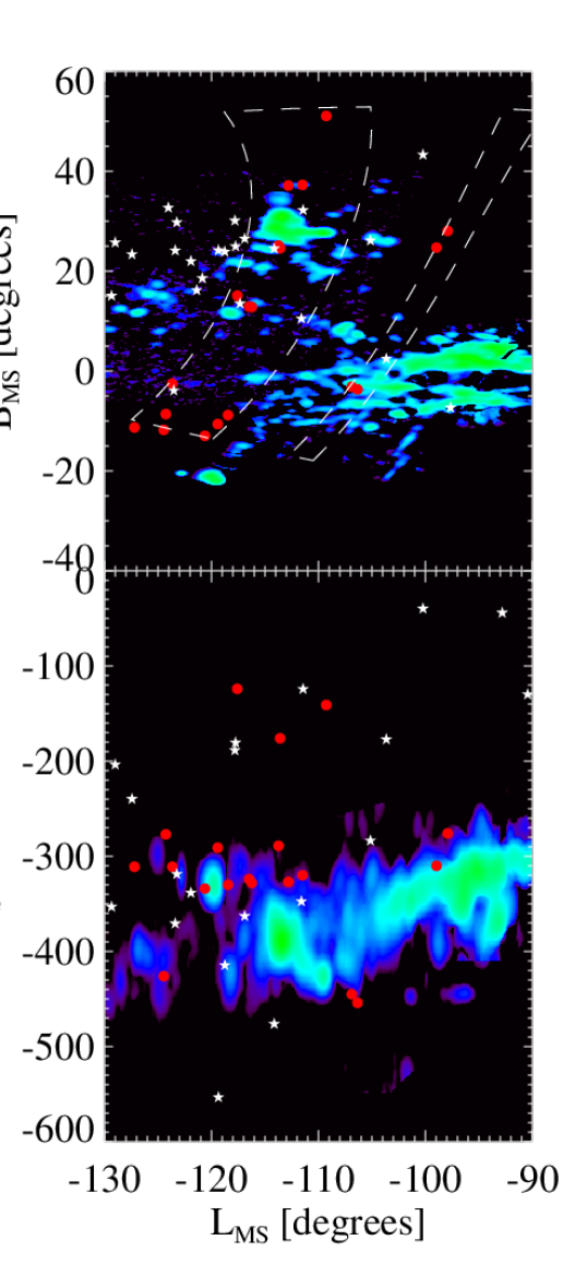
Figure 11.— A zoomed in view of the fall UCHVCs relative to the MS from Nidever et al. (2010). Symbols, shading, and panels are the same as in previous figure.

For the $\alpha$.40 footprint, the fall sky overlaps the tail of the MS and the spring sky is near the known edge of the LA but not contiguous to it. N10 extended the known tail of the MS and pointed out its complexity (see their Figure 4), so we must be especially careful with UCHVCs in the fall sky. In Figure 10, we show the UCHVCs plotted on the 200^∘ MS presented in N10. The coordinates are the MS-coordinate system of Nidever et al. (2008) based on fitting a great circle to the MS, where L_MS is the longitude along the MS and B_MS is the latitude above/below the MS. The UCHVCs are shown as large symbols (red in the online version) to increase their visibility; they are not shown to physical scale nor do their colors match the shading of the MS. The top panel shows the HI column density of the MS ($\log N_{HI}$ in cm^-2). The bottom panel is the total intensity of the MS integrated along $B_{MS}$ (K deg).

In the spring sky, the $\alpha$.40 footprint approaches but does not overlap the LA of the MS. This lack of direct coverage of the MS makes it a challenge to answer the question: could the UCHVCs be connected to the LA? Future surveys directed at determining any possible continuation of the LA will be able to directly answer this question. Until then, the key to answering this question is determining whether the UCHVCs have compatible velocities to be an extension of the LA. Clearly, the large velocity spread of UCHVCs seen in the bottom panel of Figure 10 appears to be incompatible with all of the UCHVCs being associated with the LA. Examining models of the MS can provide insight into these questions. Connors et al. (2006) model the MS as a tidal structure via interaction with the MW and LMC; they predict that the LA extends to L_MS $\sim$150^∘  with a velocity turn over starting from L_MS$\sim$60^∘ at $v_{LSR}$$\sim$300 km s^-1 extending to $\sim$-150 km s^-1. In contrast, Besla et al. (2010) simulate a first passage of the Magellanic Clouds and find a MS that extends to L_MS$\sim$50^∘ with a velocity increasing with L_MS from $v_{LSR}$$\sim$200 to 400 km s^-1. If the Connors et al. (2006) model correctly represents the history of the MS, then the clouds located at $v_{LSR}$ < 0 km s^-1 could be associated with the LA of the MS. If the Besla et al. (2010) model is accurate, then the UCHVCs are generally at higher L_MS values than predicted by the model but a few of the positive velocity clouds with $L_{MS}$ < 100^∘ and the highest $v_{LSR}$ values may be associated with the MS. For whichever model of the MS is chosen, some of the UCHVCs could be associated with the LA, but given the large spread in $v_{LSR}$ of the UCHVCs, it is impossible to associate all of the UCHVCs with the LA.

In the fall sky, the $\alpha$.40 footprint overlaps the extension of the MS detailed in N10. In Figure 11 we offer a zoomed in view focusing on the fall UCHVCs compared to the MS from N10. Here, there clearly appears to be strong overlap between the UCHVCs and the known MS system. The three clouds in the fall sky at $v_{LSR}$ > -200 km s^-1 appear to be kinematically separated from the MS. Two other clouds at L_MS $\sim$-100^∘ appear to potentially be spatially separated from the MS but the apparent separation could easily be a result of the coverage of observations of the MS. However, it is still possible that some of these UCHVCs do indeed represent galaxies. Many of the UCHVCs that overlap with the MS are also in the direction of the M31 subgroup. Disentangling the gas of known galaxies at a similar velocity from the MS is a long standing problem; see Grcevich & Putman (2009) for illustrative examples. This is also illustrated in Figure 11, where several LG galaxies are spatially and kinematically coincident with the MS.

4.2. UCHVCs in the Context of Galactic Halo Clouds

Previous studies have uncovered a population of compact clouds associated with the Galactic halo (e.g. Lockman, 2002; Lockman & Pidopryhora, 2005; Stil et al., 2006; Stanimirović et al., 2006; Ford et al., 2010; Dedes & Kalberla, 2010). While well separated from the Galactic hydrogen, these clouds typically have low $v_{LSR}$ values, and they generally appear to be consistent with Galactic rotation. The Galactic halo clouds with the most extreme velocities of Stil et al. (2006) have $v_{LSR}$ ranging from $\lesssim$100 km s^-1 to 165 km s^-1. The compact halo clouds also tend to be cold clouds, with the vast majority of reported clouds having $W_{50}$ < 10 km s^-1. Given these characteristics of the halo clouds, the UCHVCs appear as a distinct population. The UCHVCs appear to universally be warm clouds with linewidths greater than 15 km s^-1. In addition, many of the UCHVCs have substantial velocities ($|$$v_{LSR}$$|>200$ km s^-1) that are difficult to account for in a Galactic halo model.

4.3. UCHVCs in the Context of the Small Cloud Population of GALFA-HI

GALFA-HI is a survey of neutral hydrogen in the Galaxy which, like ALFALFA, uses the ALFA multi beam receiver on the Arecibo 305m antenna. For GALFA-HI, the IF signal is sent to a different spectrometer than that used by ALFALFA and is restricted to a $\sim$7 MHz bandpass centered on 1420 MHz. As a result, the GALFA-HI survey has a velocity resolution of 0.184 km s^-1  and covers a velocity range of $\pm$700 km s^-1. It should be noted that much of the GALFA data is taken commensally with the ALFALFA data through the TOGS program. Hence comparison of the results of the two surveys provides a check on our signal processing approach. Begum et al. (2010) presented an initial catalog of compact clouds from the GALFA-HI survey, and Saul et al. (2012, hereafter S12) recently released a catalog of compact clouds for the full initial data release of the GALFA-HI survey. Herein we focus on the compact clouds of S12 as the most extensive catalog of the compact cloud population discovered in the GALFA-HI survey and examine how the UCHVCs of this work are related.

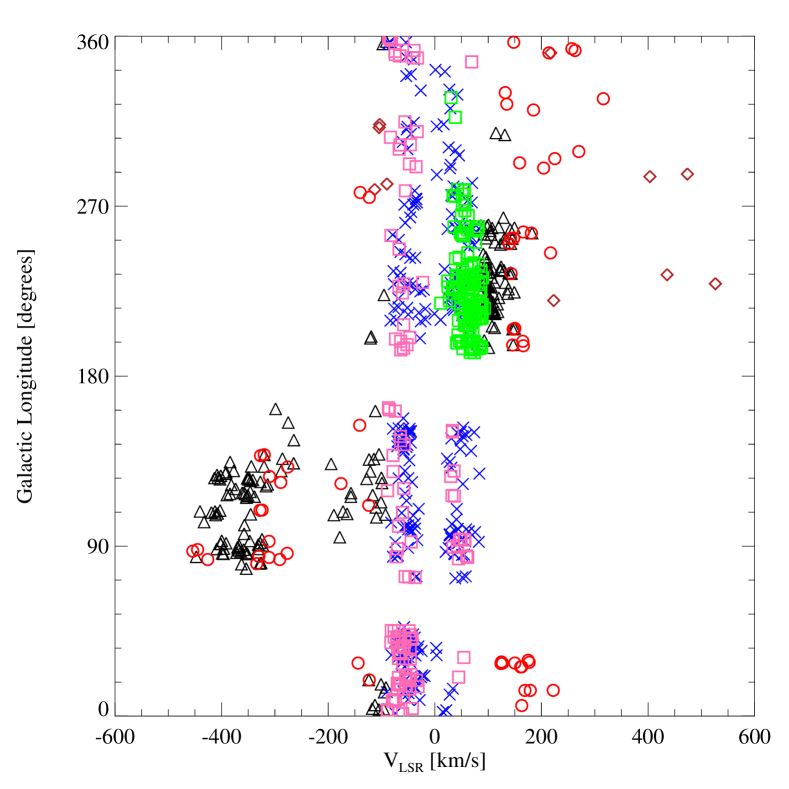
Figure 12.— The distribution of UCHVCs in $v_{LSR}$$-l$ space compared to the compact cloud populations of GALFA. Symbols and coloring follow those used in S12: Xs (blue in online version) are the cold low velocity clouds, black squares (pink in the online version) are warm low velocity clouds, grey squares (green in the online version) are the warm low velocity clouds in the third Galactic quadrant, black triangles are the high velocity clouds, and diamonds (dark red in the online version) are the galaxy candidates. The UCHVCs of this work are shown as circles (bright red in the online version).

The initial major differences to note between the catalog of S12 and the UCHVCs are additional selection criteria for the UCHVCs: the limited range of velocities considered and the strong isolation criteria. A vast majority of the compact clouds from S12 do not meet these additional criteria. S12 note several populations of clouds in their catalog which they classify by velocity, linewidth and isolation. They split between warm and cold clouds at a linewidth of 15 km s^-1, or a temperature of $\sim$5000 K. It should be noted that while ALFALFA does not have the velocity resolution of the GALFA-HI survey, the velocity resolution of $\sim$10 km s^-1 is sufficient to distinguish warm from cold clouds; as can be seen in Figure 8, the UCHVCs are all warm clouds with linewidths greater than 15 km s^-1. S12 also split their clouds into low velocity and high velocity populations at $|$$v_{LSR}$$|=$90 km s^-1. They find a few cold clouds with $v_{LSR}$ > 90 km s^-1, but the vast majority of their cold clouds are at lower velocities and associated with the Galactic disk, a very distinct population from the ALFALFA UCHVCs. The populations from S12 of most relevance to this work are their HVC population ($|$$v_{LSR}$$|$ > 90 km s^-1) and galaxy candidate population; both of these populations are generally composed of warm clouds. The difference between the HVC population and galaxy candidate population of S12 is that the galaxy candidates have an additional stringent isolation criterion (different from the isolation criteria used here) and hence are the population most directly comparable to the UCHVCs. In Figure 12, we compare the distribution of the UCHVCs to the compact clouds of S12 in galactic longitude versus $v_{LSR}$. In the second Galactic quadrant, the UCHVCs overlap with the HVCs of S12. This corresponds to the fall sky, and, as noted in the previous section, when considering a stricter isolation criterion for separation from larger HVC complexes akin to that used by S12, the fall UCHVCs cannot be considered isolated structures. In the first and fourth Galactic quadrants, the UCHVCs as a population appear separated from the compact clouds of S12. The positive velocity clouds in the first quadrant and the clouds (at both positive and negative velocities) in the fourth quadrant have no HVC population counterpart in the GALFA compact cloud catalog. Especially in the fourth quadrant, there are multiple clouds at substantial velocites ($v_{LSR}$ > 200 km s^-1) that appear well separated from other clouds populations.

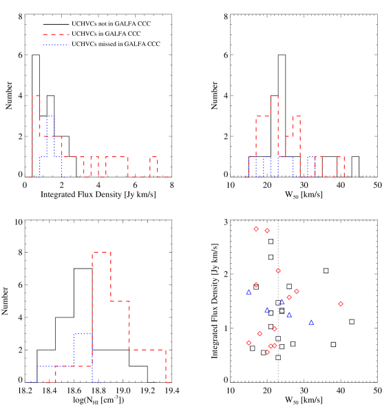
Figure 13.— Properties for the UCHVCs not seen in the GALFA-HI dataset (solid lines/squares; black in the online version), UCHVCs included in the GALFA compact cloud catalog (CCC) of S12 and those found by the identification algorithm but discarded from the final catalog (dashed lines/diamonds; red in the online version), and UCHVCs seen in the GALFA-HI dataset but missed by the cloud finding algorithm of S12 (dotted lines/trianges; blue in the online version). The dotted line in the bottom right panel indicates the median velocity width of the UCHVCs.

As a check of our methodology and dataset, we also perform a direct comparison of the ALFALFA UCHVCs to the catalog of S12. First, we examine which of the S12 galaxy candidates appear in the $\alpha$.40 catalog. S12 find 28 HVCs that they consider extremely isolated and which they classify as galaxy candidates. Of these, 10 are within the $\alpha$.40 footprint. Two of the GALFA galaxy candidates are classified as extragalactic sources in $\alpha$.40 (AGC191803 and AGC227874) and are clearly associated with optical counterparts; a third S12 galaxy candidate is associated with UGC 7753, a large barred spiral galaxy. Four of their galaxy candidates are within the ALFALFA data but have $|$$v_{LSR}$$|$ < 120 km s^-1 and are not included in this work (one is included in they $\alpha$.40 catalog, AGC238801). One of the galaxy candidates is also included here in the UCHVC catalog – HVC351.17+58.56+214. Two of the S12 galaxy candidates are not seen in the ALFALFA data; these are both lower S/N sources (S/N < 7) and one is extremely narrow velocity width ($W_{50}=$ 3.9 km s^-1).

Secondly, we can examine the UCHVCs for counterparts in the S12 catalog. 11 of the 59 UCHVCs are included in the GALFA compact cloud catalog, of which one (HVC351.17+58.56+214) is classified by S12 as a galaxy candidate; the other ten are included in their HVC sample. Seventeen of the UCHVCs are not included in the data coverage of the GALFA DR1 release (D. Saul, private communication); these sources are in the spring sky region of $\delta=8-16$^∘, where GALFA DR1 has limited coverage because GALFA-HI observations started one year after the commencement of ALFALFA data taking and hence commensal data for that time period are missing. Of the thirty-one UCHVCs with GALFA coverage not contained within the catalog of S12, eight of these sources are found by the algorithm but discarded due to either failing the S12 criteria or data quality issues, such as noise spikes. Five are seen in the data but not found by the signal identification algorithm of S12. The last eighteen are not visible in the GALFA-HI data (D. Saul, private communication 2013). In Figure 13, we explore the differences in properties between the UCHVCs found in the dataset of GALFA-HI by the signal identification algorithm of the S12 (including sources discarded from the final catalog), the UCHVCs visible in the GALFA data but not identified by their automated algorithm, and the UCHVCs not visible in the GALFA data. Most strikingly, there is a bimodal distribution in the average column density with the UCHVCs not visible in the GALFA-HI data having the lowest average column densities. In addition, there is a velocity width effect; generally the UCHVCs identified within the GALFA dataset are the narrowest velocity width sources. In the bottom right panel of Figure 13, we focus on UCHVCs with integrated flux densities less than 3 Jy km s^-1 as the higher flux sources are all detected in the GALFA-HI data. Then, there are 18 UCHVCs with linewidths greater than 23 km s^-1, the median $W_{50}$ of the full sample. Of these, only three are identified in the GALFA-HI dataset and those still tend to be among the highest flux objects with integrated flux densities greater than 1.45 Jy km s^-1, above the median value of 1.34 Jy km s^-1. The UCHVCs that are identified within the GALFA dataset that have flux densities below the median value of the UCHVC sample also have linewidths narrower than the median value of the UCHVCs. This is a straightforward result of the different focus of the two surveys; the GALFA-HI data are designed to detect narrow velocity width HI features associated with Galactic hydrogen while the ALFALFA dataset is designed to detect extragalactic HI sources with wider linewidths. While we will address the completeness and reliability of the UCHVC catalog in future work, we note that six UCHVCs not included in the GALFA catalog have all been confirmed as real HI signals via confirmation observations with the Arecibo L-Band Wide receiver (Adams et al. in prep). In addition, the UCHVCs presented here have strict S/N criteria so the likelihood that many of the UCHVCs are false detections is small. This demonstrates the utility of the ALFALFA dataset, detection algorithm presented here, and the source inspection.

5. UCHVCs as Minihalo Candidates

The mismatch between observations of low mass galaxies and simulations of dark matter halos remains an outstanding question in understanding both the cosmological paradigm and galaxy formation and evolution. Is the $\Lambda$CDM paradigm incorrect? How does star formation and gas accretion proceed in the lowest mass halos? Finding the lowest mass dark matter halos with baryons can help address these question. In this section, we discuss the possibility that the UCHVCs presented in this paper could represent gas-bearing minihalos. In this context, a minihalo is dark matter halo below the critical mass of $\sim 10^{10}$ $M_{\odot}$ where astrophysical processes begin to strongly affect the baryon content (e.g. Hoeft & Gottlöber, 2010; Hoeft et al., 2006)

Sternberg et al. (2002) examined in detail how neutral hydrogen could exist in minihalos. They found that the neutral gas would be surrounded by an envelope of ionized gas, with the specifics depending upon the pressure of the ionized medium the halo is immersed in. They examined both cuspy (NFW) and constant density (Burkert) cores. Cuspy cores are predicted by simulations, while observations of dwarf galaxies indicates that low mass dark matter halos have constant density cores. The UCHVCs appear to match well the Sternberg et al. (2002) minihalo models with a median Burkert density profile, $D_{HI}\simeq 1.4$ kpc, $M_{HI}\simeq 3\times 10^{5}\ M_{\odot}$, total to neutral gas mass ratio of 15, peak $N_{HI}\simeq 4\times 10^{19}\,\mathrm{cm}^{-2}$, total halo mass $M_{vir}\simeq 3\times 10^{8}\ M_{\odot}$, surrounded by a hot, ionized IGM of pressure $P_{HIM}=10\,\mathrm{cm}^{-3}$ K. The measured column densities are averaged over the size of the cloud and smeared by the 3^′.5 beam of the Arecibo telescope and hence represent a lower limit to the true peak column density, and so they are consistent with the higher peak $N_{HI}$ values of the model. The measured $M_{dyn}$ is an estimate of the total mass within the HI extent; the total size of the dark matter halo exceeds the HI size by a factor of several, explaining the discrepancy between the total halo mass of the model and the inferred dynamical mass from ALFALFA. Work is ongoing to match the individual UCHVC detections to specific individual models (Y. Faerman et al., submitted).

5.1. Previous Searches for Minihalos

A LG origin for HVCs, or at least a subset of the HVC population has been considered before. With the advent of large-scale, sensitive, blind HI surveys, interest was revived in HVCs as tracers of dark matter halos. Blitz et al. (1999) and Braun & Burton (1999) both postulated a LG origin for HVCs; Braun & Burton (1999) specifically proposed that compact HVCs (CHVCs), identified by their isolation and undisturbed spatial structure, were good candidates to represent dark matter halos throughout the LG. de Heij et al. (2002b) extracted a set of CHVCs from the Leiden/Dwingeloo Survey (LDS), and Putman et al. (2002) similarly presented a set of CHVCs from the HI Parkes All-Sky Survey (HIPASS). Further work, both observational and theoretical, since the discovery of the CHVC population suggests that they most likely represent a circumgalactic population. The properties of the CHVC population from the two catalogs are summarized in Table 5. Sequentially, this table lists: object class, distance (in kpc), HI angular diameter (in arcmin), HI diameter (in kpc), peak column density, $W_{50}$, integrated flux density, HI mass, and dynamical mass within the HI extent. de Heij et al. (2002a) showed that the properties of the CHVCs for the two datasets are the same when accounting for the better spatial resolution and sensitivity of HIPASS and the better velocity resolution of LDS.

Sternberg et al. (2002) and Maloney & Putman (2003) independently modeled gas in dark matter halos to understand the CHVC population. Based on considerations of their astrophysical properties, both groups concluded that the best interpretation of the CHVCs was as circumgalactic objects at $d\lesssim 200$ kpc. Sternberg et al. (2002) found that if the CHVCs were at $d>750$ kpc, their dark matter halos were extremely underconcentrated. They found that at $d\lesssim 150$ kpc, the CHVCs were consistent with being gas pressure confined in dark matter halos. In this scenario, the CHVCs represent the subhalos surrounding the Milky Way from its hierarchical formation. Both pointed out that the gas of the CHVCs must be largely ionized, implying that the total mass of gas is much greater than the observed mass. If the CHVCs were at distances of 0.7-1 Mpc, extremely low dark-matter-to-gas ratios would then be required to match the observed linewidths of the CHVCs, and they would violate the $\Lambda$CDM mass-concentration relation. They argued that the CHVCs must be at $d\lesssim 200$ kpc to match size and total dark matter constraints. More recent observational evidence also indicates that the CHVCs must be at circumgalactic distances. The HI masses of the CHVCs at LG distances of $\sim$1 Mpc are a few times $10^{7}$ $M_{\odot}$, large enough that they should have been detected in surveys of other galaxy groups but have not (e.g. Pisano et al., 2007; Chynoweth et al., 2011a; Zwaan, 2001; Braun & Burton, 2001; Pisano et al., 2004). In addition, higher resolution observations of CHVCs show clear ram pressure indicators in many cases, indicating that the CHVCs are located at circumgalactic distances (Westmeier et al., 2005b). Observations of potential CHVC analogs around M31 also point to a circumgalactic origin. Westmeier et al. (2005a) studied HVCs associated with M31 in high resolution; importantly, the association of these HVCs with M31 allows a distance constraint to be derived. As outlined in Table 5, the properties of the M31 HVCs are a good match to the properties of the CHVCs at $d\sim 150$ kpc, indicating that the two samples are likely a similar population.

Table 5HI Content in the LG - HVCs and Galaxies

Class	d	$\theta$	$D_{HI}$	$N_{HI}$	$W_{50}$	$S_{21}$	$M_{HI}$	$M_{tot}$	Refs
	kpc	′	kpc	atoms $\mathrm{cm}^{2}$	km s-1	Jy km s-1	$M_{\odot}$	$M_{\odot}$
UCHVCs	$d=1000$	10	2.9$d$	$\gtrsim 0.6\times 10^{19}$	23	1.26	$1.8\times 10^{5}\,d^{2}$	$3.3\times 10^{7}\,d$	1
CHVCs (LDS)	150	60	2.6	$1.3\times 10^{19}$	25	102	$5.4\times 10^{5}$	$3.5\times 10^{7}$	2
CHVCs (HIPASS)	150	24	0.52	$1.4\times 10^{19}$	35	19.9	$1.1\times 10^{5}$	$2.7\times 10^{7}$	3
M31 HVCs	780	4.6	1.04	$3.9\times 10^{19}$	24	2.1	$3.0\times 10^{5}$	$4.5\times 10^{7}$	4
Leo T	420	5	0.6	$70\times 10^{19}$	16	6.7	$2.8\times 10^{5}$	$.33\times 10^{7}$	5
Leo P	$1750$	2.0	1.0	$20\times 10^{19}$	24	1.31	$9.5\times 10^{5}$	$1.3\times 10^{7}$	6,7,8

Multiple searches have been undertaken for minihalos around nearby galaxy groups (e.g. Zwaan, 2001; Braun & Burton, 2001; de Blok et al., 2002; Minchin et al., 2003; Barnes & de Blok, 2004; Pisano et al., 2004, 2007, 2011; Chynoweth et al., 2009; Kovač et al., 2009; Irwin et al., 2009; Chynoweth et al., 2011a, b; Mihos et al., 2012). Generally, these surveys must choose between sensitivity and coverage area. Irwin et al. (2009) undertook a deep survey of the nearby isolated galaxy NGC 2903 sensitive to an HI mass of $2\times 10^{5}$ $M_{\odot}$ and covering 150 kpc $\times$ 260 kpc. This survey was sensitive enough to (barely) detect a Leo T analog but given that the survey footprint only extends to $\sim$100 kpc in projected radius from the galaxy center, detection of an object at $\gtrsim$400 kpc from the galaxy center would depend strongly on orientation. Irwin et al. (2009) did detect one minihalo with an HI mass of $2.6\times 10^{6}$ $M_{\odot}$, a comparable stellar stellar mass and a dynamical mass of $\gtrsim 10^{8}$ $M_{\odot}$. Chynoweth et al. (2011b) undertook a large (480 kpc $\times$ 1.2 Mpc; 8^∘.7 $\times$ 21^∘.3) survey centered on the region between the M81/M82 and NGC 2403 galaxy groups. Their survey had a mass detection limit of $3.2\times 10^{6}$ $M_{\odot}$which is not deep enough to detect a Leo T analog. While their survey covers a large footprint, it is focused on the region between two connected galaxy groups and coverage of the outskirts of the galaxy groups is limited. They detect several massive HI clouds (M > $10^{6}$ $M_{\odot}$) and determine that these clouds likely arise from tidal processes given their clustering near M81. Mihos et al. (2012) surveyed the M101 group over 1050 $\times$ 825 kpc (8^∘.5 $\times$ 6^∘.7) to a mass senstivity of varying from 2 to 10 $\times 10^{6}$ $M_{\odot}$ over their footprint. This footprint includes all objects out to $\sim$400 kpc from the central galaxy, regardless of orientation, but the survey is not sensitive enough to detect a Leo T analog. They do identify a new low surface brightness dwarf galaxy through an HI detection and a starless HI cloud with an HI mass of $1.2\times 10^{7}$ $M_{\odot}$.

5.2. Known Minihalos in the LG

In considering the UCHVCs as gas-bearing minihalos in the LG, we first want to examine the context of the LG and ask what we may empirically expect a minihalo to look like. The population of the LG has increased substantially in the last few years with the discovery of the UFD satellites of the Milky Way from automated stellar searches of the Sloan Digital Sky Survey (Willman, 2010) and targeted searches for satellites of M31 (e.g. Ibata et al., 2007; McConnachie et al., 2009). The UFDs have indicative dynamical masses within the baryon extent of $10^{6}-10^{7}$ $M_{\odot}$ and most likely inhabit dark matter halos that qualify them as minihalos. With the exception of Leo T and the recently discovered Leo P, the UFDs are located within the virial radius of the MW or M31 and have no detectable gas content.

Surveys of low mass galaxies in the field indicate that, with large scatter, dwarf galaxies tend to be gas-rich and can have atomic gas as their dominant baryon component (e.g. Geha et al., 2006; Schombert et al., 2001). Modulo the uncertainties in how astrophysical processes affect the baryon content of the lowest mass halos, one would naively expect the trend of high gas fraction to continue as lower mass galaxies are discovered. Leo T is the only UFD discovered through optical surveys that has neutral gas content; it is also the UFD that is most distant from the MW. The other UFDs are located within the virial radius of the MW or M31 and many show signs of tidal interaction with the MW (e.g. Sand et al., 2012).Grcevich & Putman (2009) find that morphological segregation is strong in the LG with dwarf galaxies within 270 kpc of the Milky Way or Andromeda showing no evidence of neutral gas content. Leo T is on the edge of detectability for SDSS; were it located further away, its stellar population would not have been detected (Kravtsov, 2010). Taken together, these facts raise the possibility that more gas-rich UFDs are lurking in the LG with distances and stellar populations that would leave them undetected in SDSS.

Leo T serves as our prototype of what a gas-rich minihalo will look like; it has motivated our search for more minihalos and the discovery of Leo P. In Figure 14 we examine the HI properties of the LG galaxies and neighboring dwarf galaxies within 3 Mpc in comparison to Leo T and Leo P to infer what we may expect for future minihalo detections. The top panel of Figure 14 shows a histogram of the HI masses of dwarf galaxies within the LG and neighboring systems, taken from McConnachie (2012). Leo P and Leo T have some of the lowest HI masses in the LG and Local Volume (LV); we would expect previously undetected systems to have low HI masses. The bottom panel of Figure 14 illustrates the parameter space occupied by Leo T and Leo P in the LG and LV; they have low HI masses and low dynamical masses.

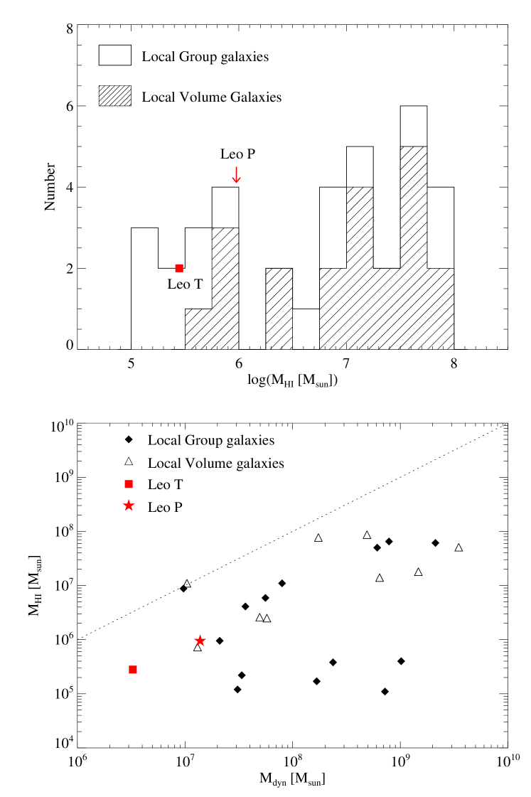
Figure 14.— The top panel is a histogram of HI mass in the LG and nearby dwarf galaxies in the Local Volume (indicated by the hashed histogram), including Leo T (its contribution indicated by the red filled square), from the catalog of McConnachie (2012). The location of Leo P is also indicated. The bottom panel is HI mass as a function of dynamical mass within the baryon extent. The diamonds are LG galaxies with HI content, the triangles Local Volume dwarfs, the filled square is Leo T and the filled star is Leo P. The dynamical masses are compiled from the literature and are calculated using a variety of different methods and at different extents of the galaxies; in all cases the dynamical masses are underestimates of the true dynamical mass (Łokas, 2009; De Rijcke et al., 2006; Geha et al., 2010; Shostak & Skillman, 1989; Cook et al., 1999; Hoffman et al., 1996; Mateo, 1998; Ryan-Weber et al., 2008; Kepley et al., 2007; Begum & Chengalur, 2004; Kirby et al., 2012; Skillman et al., 1988; Begum et al., 2005, 2006). The dotted line indicates where M_dyn equals M_HI. In addition to having low HI masses, Leo T and Leo P also have low dynamical masses.

5.3. Evidence for the UCHVCs as Minihalo Candidates

In assessing the UCHVCs as minihalo candidates, we first consider if their astrophysical properties are consistent with the scenario. As mentioned above, the UCHVCs are a good match to the models of Sternberg et al. (2002). Importantly, the UCHVCs also overcome the objections that ruled out the CHVCs as minihalo candidates throughout the LG. As summarized in Table 5, the UCHVCs have HI masses typical of $\sim 10^{5}\,d^{2}$ $M_{\odot}$ and HI diameters of $\sim 2.9\,d$ kpc. These smaller sizes and lower fluxes suggest that at distances of 1 Mpc, the physical properties of the UCHVCs are good matches to the CHVC properties at distances of $\sim$250 kpc. In this scenario, the CHVCs could represent subhalos within the MW and the UCHVCs represent isolated structures within the LG.

The LG is a bound group of galaxies, hence studying the kinematics of the UCHVCs can help constrain their association with the LG. In Figure 15 we compare the motions of the UCHVCs to the LG. Following Courteau & van den Bergh (1999), we plot $v_{\odot}$ versus the cosine of the angle from the LG apex. In general the UCHVCs show similar behavior to the motions of the LG galaxies, lending credence to the possibility that they trace LG dark matter halos. They do appear to have a higher velocity dispersion, similar to the nearby neighbor galaxies that are not bound to the LG. This may suggest that the UCHVCs are outlying systems, marginally bound to the LG.

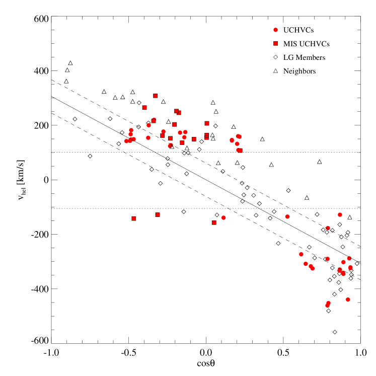
Figure 15.— Cosine of the angle from the Solar apex versus heliocentric velocity. The solid line shows the relation of Courteau & van den Bergh (1999) and the dashed lines are their stated error. The dotted lines indicate inaccessible velocity space due to the UCHVC velocity selection criterion. The filled circles (red in the online version) are the UCHVCs with the outlined filled squares (red in the online version) indicating the MIS UCHVCs. The diamonds are the LG galaxies from McConnachie (2012) and the triangles are neighboring galaxies within 3 Mpc that are not bound to the LG.

Finally, we offer a preliminary comparison of the UCHVCs to the Via Lactea II (VL) simulation of Diemand et al. (2008), a high resolution cosmological N-body simulation of a Milky Way analog. We compare the spatial and kinematic distribution of the UCHVCs to the dark matter halos of the VL simulation to see if the hypothesis of UCHVCS as minihalos is consistent with theoretical predictions. We utilize the full volume of the simulation, which includes 20,048 halos that extend to more than 3 Mpc from the central MW analog halo. In addition to the central massive halo, there is a second massive halo which is a fortuitous analog to M31 (Teyssier et al., 2012). In our favored model, we place this second massive halo at the approximate location of M31 in order to most closely match the LG. We also use the original simulation coordinates plus five random orientations of the subhalos to demonstrate the importance of structure within the LG. After the coordinate transformations, we only consider the halos within the simulation that lie within the boundaries of the $\alpha$.40 coverage and meet our velocity criterion.

In Figure 16 we show the distribution of galactic latitude and $v_{LSR}$ for the UCHVCs and the VL subhalos. Due to the presence of large and complex HVC structure in the fall sky, we focus on the spring sky for our comparison. In the left column we show all the halos that match our selection criteria; in the right column we show only those halos located further than 250 kpc from the central massive halo to more closely approximate the halos we expect to be gas-bearing. The effects of structure are much more noticeable when only the most distant halos are considered; the different orientations show a much wider spread in the distribution of $|b|$ in this case. The galactic latitude plot is especially important as it provides a quick test of whether the distribution of clouds is within the Galactic disk or a circumgalactic distribution. If the UCHVCs are associated with the Galactic disk, a flattened distribution of $|b|$ values is expected compared to the case if the UCHVCs are distributed around the Galaxy. The UCHVCs and MIS UCHVCs have similar distributions for $|b|$ and $|$$v_{LSR}$$|$. The favored orientation of the VL simulation appears to match well the distribution of $|b|$ for the UCHVCs. The large differences in the cumulative distribution function (CDF) of $|b|$ for the random orientations shows the importance of structure. The kinematics of the UCHVCs appear to be consistent with the VL simulation in all cases with the CDF of $|$$v_{LSR}$$|$ matching well in all cases. While it is beyond the scope of this paper to do a full halo-population analysis, the rough analysis presented here shows that the UCHVCs agree reasonably well with the VL simulation.

We can also use the VL simulations to provide a rough check of the numbers of halos expected. There are 40 UCHVCs in the spring sky, including 17 in the most-isolated subsample. We compare to our favored orientation of the VL simulation, noting that it matches the spring sky in that we are looking into the outskirts of the simulation as the spring region of ALFALFA probes the outskirts of the LG. There are a total of 168 VL halos that meet our velocity criterion in the region of the simulation that matches the $\alpha$.40 spring footprint. When limited to halos with distances from the central MW analog halo greater than 250 kpc, there are a total of 44 halos; 27 of these halos have $M_{tidal}>10^{7}$ $M_{\odot}$. Given the roughness of our numbers the two populations appear to be consistent.

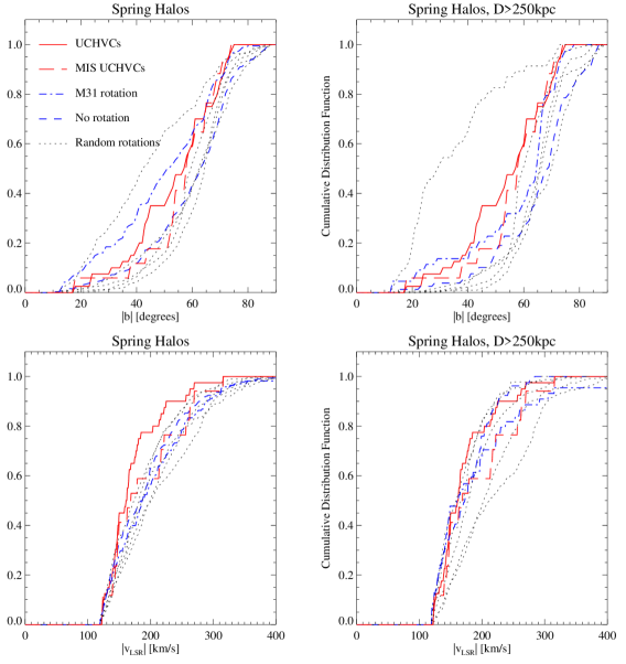
Figure 16.— The distribution of subhalos from the Via Lactea II simulation compared to the UCHVCs (solid line, red in the online version) and the most-isolated subsample (dashed line, red in the online version). The dot-dash line (blue in the online version) represents the subhalos in the original simulation coordinate system; the dashed line (blue in the online version) is our favored orientation where the simulation rotated to place the second massive halo at the approximate location of M31. The dotted lines represent five random rotations of the simulation coordinates. The left-hand column shows the distribution of all the VL subhalos in the spring footprint that meet our velocity criterion, and the right-hand column shows the VL subhalos that are located further than 250 kpc from the central massive halo. Overall, the UCHVCs appear consistent with the distribution of halos from the simulation, especially for our favored orientation. Given the large differences between halo distribution depending on the rotation of the simulation coordinates, it is clear that accounting for structure is crucial.

5.4. The UCHVCs as Galaxies

As galaxies, the UCHVCs would favor the outskirts of the LG, rather than the central regions, with distances of $\sim$500 kpc – 1 Mpc. They would have HI masses of $\sim 10^{5}$ $M_{\odot}$ with envelopes of warm ionized hydrogen with masses of $\sim 10^{6}$ $M_{\odot}$. The indicative dynamical masses within the HI extent are $\sim 10^{7}-10^{8}$ $M_{\odot}$, and the total hosting halo masses are likely $\gtrsim 10^{9}$ $M_{\odot}$. While this hypothesis is attractive, it cannot be definitively proven until distance constraints are in place for the UCHVCs. Further work is necessary in order to constrain their distances as the ALFALFA HI detection carries no direct distance information. The kinematics of the UCHVCs are dominated by LG interactions, so the velocity cannot offer any insights to the distance. The detection of an optical counterpart can constrain the distance through studies of the stellar population. It is also possible to constrain the distance solely through HI by using synthesis imaging to determine the rotational velocity of the UCHVCs and constrain the distance through the baryonic Tully-Fisher relation (e.g. Giovanelli et al., 2013; McGaugh, 2012). An alternative to confirming the distance of the UCHVCs directly is to detect UCHVC analogs around other nearby galaxy groups and use the association with the group to constrain the distance and properties of the clouds. Planned future HI surveys using phased-array-feeds will be able to robustly detect these objects.

Confirming that a subset of the UCHVCs are galaxies will offer many insights. The UCHVCs will increase the number of low-mass galaxies known in the Local Volume, decreasing the discrepancy between simulations and observations. In addition, the UCHVCs will trace the outskirts of the LG allowing the comparison between simulations and observations to be extended to a larger volume. The UCHVCs will also serve as isolated examples of the lowest mass galaxies, having not yet interacted substantially with the MW. The UCHVCs offer the potential to study star formation in extreme, low metallicity environments as the presence of gas means there is a possibility of star formation. In fact, Leo T has recently formed stars and Leo P has ongoing star formation with one HII region. Abundance measurements of the HII region in Leo P indicate that it is among the lowest metallicity systems known and blind HI surveys may prove to be a promising way to detect low luminosity, extremely metal deficient galaxies (Skillman et al., 2013).

The two confirmed low mass gas-rich galaxies in the Local Volume, Leo T and Leo P, both have high average column densities and small HI angular diameters, as can be seen in Figures 8 and 9. It may be reasonable to expect then that the most compact and highest column density UCHVCs are the best candidates to represent low-mass gas-rich galaxies. HVC274.68+74.70-123, HVC351.17+58.56+214, and HVC13.59+54.52+169 are in the most-isolated subsample, have average angular diameters < 7^′, and have $\bar{N}_{HI}>10^{19}\,\mathrm{cm}^{-2}$; we suggest that these are the best galaxy candidates in our sample. One of these candidates, HVC351.17+58.56+214 is also identified by the GALFA-HI survey as a good galaxy candidate. Notably, it is among the most compact clouds included in this catalog (7^′ $\times$ 5^′) and has one of the highest column densities ($\log~{}\bar{N}_{HI}=19.3$). If we adopt a representative distance of 1 Mpc, it has a HI mass of $3.9\times 10^{5}$ $M_{\odot}$ and an indicative dynamical mass within the HI extent of $2.1\times 10^{7}$$M_{\odot}$.

6. Conclusion

We present a set of 59 ultra-compact high velocity clouds which are of interest as speculative minihalo candidates. In brief, the properties of the UCHVCs are summarized below.

• They have HI integrated flux densities from 0.66–8.55 Jy km s^-1 with a median of 1.34 Jy km s^-1, linewidths of 15–70 km s^-1 with a median of 23 km s^-1, and angular diameters of 4–20^′ with a median of 10^′.

• They are selected according to strict isolation criteria. As a result, they are distinct from known HVC populations.

• Their HI sizes and HI fluxes allow them to overcome previous objections leveled against CHVCs as LG minihalos.

• They are consistent with the minihalo models of Sternberg et al. (2002). At a distance of $\sim$1 Mpc, they have HI masses of $10^{5}-10^{6}$ $M_{\odot}$ and dynamical masses within the HI extent of $10^{7}-10^{8}$ $M_{\odot}$. Their total gas masses, including the surrounding ionized envelope, would be $\sim 10^{6}-10^{7}$$M_{\odot}$ and the total hosting halo masses would be $\lesssim 10^{9}$ $M_{\odot}$.

• As galaxies, they would allow us to probe the outskirts of the LG, study low mass systems that have remained isolated from the MW, and provide an avenue for indentifying extremely metal deficient galaxies.

We thank David Nidever for providing his dataset of the Magellanic Stream, Bart Wakker for providing the updated HVC catalog and useful comments, Destry Saul for help in comparing the UCHVCs to the GALFA-HI dataset, and the anonymous referee for helpful comments. The ALFALFA survey team at Cornell is supported by NSF grants AST-0607007 and AST-1107390 to RG and MPH and by grants from the Brinson Foundation. EAKA has also been supported by an NSF predoctoral fellowship.

This research has made use of NASA’s Astrophysics Data System Bibliographic Services and the NASA/IPAC Extragalactic Database (NED), which is operated by the Jet Propulsion Laboratory, California Institute of Technology, under contract with the Nataion Aeronautics and Space Administration.

References

- Barnes & de Blok (2004) Barnes, D. G., & de Blok, W. J. G. 2004, MNRAS, 351, 333
- Begum & Chengalur (2004) Begum, A., & Chengalur, J. N. 2004, A&A, 413, 525
- Begum et al. (2006) Begum, A., Chengalur, J. N., Karachentsev, I. D., Kaisin, S. S., & Sharina, M. E. 2006, MNRAS, 365, 1220
- Begum et al. (2005) Begum, A., Chengalur, J. N., Karachentsev, I. D., & Sharina, M. E. 2005, MNRAS, 359, L53
- Begum et al. (2010) Begum, A., Stanimirović, S., Peek, J. E., et al. 2010, ApJ, 722, 395
- Besla et al. (2010) Besla, G., Kallivayalil, N., Hernquist, L., et al. 2010, ApJ, 721, L97
- Blanton et al. (2005) Blanton, M. R., Lupton, R. H., Schlegel, D. J., et al. 2005, ApJ, 631, 208
- Blitz et al. (1999) Blitz, L., Spergel, D. N., Teuben, P. J., Hartmann, D., & Burton, W. B. 1999, ApJ, 514, 818
- Bovill & Ricotti (2011) Bovill, M. S., & Ricotti, M. 2011, ApJ, 741, 17
- Braun & Burton (1999) Braun, R., & Burton, W. B. 1999, A&A, 341, 437
- Braun & Burton (2001) —. 2001, A&A, 375, 219
- Cannon et al. (2011) Cannon, J. M., Giovanelli, R., Haynes, M. P., et al. 2011, ApJ, 739, L22
- Chynoweth et al. (2011a) Chynoweth, K. M., Holley-Bockelmann, K., Polisensky, E., & Langston, G. I. 2011a, AJ, 142, 137
- Chynoweth et al. (2011b) Chynoweth, K. M., Langston, G. I., & Holley-Bockelmann, K. 2011b, AJ, 141, 9
- Chynoweth et al. (2009) Chynoweth, K. M., Langston, G. I., Holley-Bockelmann, K., & Lockman, F. J. 2009, AJ, 138, 287
- Connors et al. (2006) Connors, T. W., Kawata, D., & Gibson, B. K. 2006, MNRAS, 371, 108
- Cook et al. (1999) Cook, K. H., Mateo, M., Olszewski, E. W., et al. 1999, PASP, 111, 306
- Courteau & van den Bergh (1999) Courteau, S., & van den Bergh, S. 1999, AJ, 118, 337
- de Blok et al. (2002) de Blok, W. J. G., Zwaan, M. A., Dijkstra, M., Briggs, F. H., & Freeman, K. C. 2002, A&A, 382, 43
- de Heij et al. (2002a) de Heij, V., Braun, R., & Burton, W. B. 2002a, A&A, 392, 417
- de Heij et al. (2002b) —. 2002b, A&A, 391, 159
- De Rijcke et al. (2006) De Rijcke, S., Prugniel, P., Simien, F., & Dejonghe, H. 2006, MNRAS, 369, 1321
- Dedes & Kalberla (2010) Dedes, L., & Kalberla, P. W. M. 2010, A&A, 509, A60
- Diemand et al. (2008) Diemand, J., Kuhlen, M., Madau, P., et al. 2008, Nature, 454, 735
- Dieter (1965) Dieter, N. H. 1965, AJ, 70, 552
- Evoli et al. (2011) Evoli, C., Salucci, P., Lapi, A., & Danese, L. 2011, ApJ, 743, 45
- Ford et al. (2010) Ford, H. A., Lockman, F. J., & McClure-Griffiths, N. M. 2010, ApJ, 722, 367
- Fukugita & Peebles (2006) Fukugita, M., & Peebles, P. J. E. 2006, ApJ, 639, 590
- Geha et al. (2006) Geha, M., Blanton, M. R., Masjedi, M., & West, A. A. 2006, ApJ, 653, 240
- Geha et al. (2010) Geha, M., van der Marel, R. P., Guhathakurta, P., et al. 2010, ApJ, 711, 361
- Giovanelli et al. (2013) Giovanelli, R., Haynes, M. P., Adams, E. A. K., et al. 2013, submitted
- Giovanelli et al. (2010) Giovanelli, R., Haynes, M. P., Kent, B. R., & Adams, E. A. K. 2010, ApJ, 708, L22
- Giovanelli et al. (2005) Giovanelli, R., Haynes, M. P., Kent, B. R., et al. 2005, AJ, 130, 2598
- Giovanelli et al. (2007) —. 2007, AJ, 133, 2569
- Grcevich & Putman (2009) Grcevich, J., & Putman, M. E. 2009, ApJ, 696, 385
- Guo et al. (2010) Guo, Q., White, S., Li, C., & Boylan-Kolchin, M. 2010, MNRAS, 404, 1111
- Hartmann & Burton (1997) Hartmann, D., & Burton, W. B. 1997,
- Haynes et al. (2011) Haynes, M. P., Giovanelli, R., Martin, A. M., et al. 2011, AJ, 142, 170
- Hoeft & Gottlöber (2010) Hoeft, M., & Gottlöber, S. 2010, Advances in Astronomy, 2010, 87
- Hoeft et al. (2006) Hoeft, M., Yepes, G., Gottlöber, S., & Springel, V. 2006, MNRAS, 371, 401
- Hoffman et al. (1996) Hoffman, G. L., Salpeter, E. E., Farhat, B., et al. 1996, ApJS, 105, 269
- Ibata et al. (2007) Ibata, R., Martin, N. F., Irwin, M., et al. 2007, ApJ, 671, 1591
- Irwin et al. (2009) Irwin, J. A., Hoffman, G. L., Spekkens, K., et al. 2009, ApJ, 692, 1447
- Karachentsev & Makarov (1996) Karachentsev, I. D., & Makarov, D. A. 1996, AJ, 111, 794
- Kepley et al. (2007) Kepley, A. A., Wilcots, E. M., Hunter, D. A., & Nordgren, T. 2007, AJ, 133, 2242
- Kirby et al. (2012) Kirby, E. N., Cohen, J. G., & Bellazzini, M. 2012, ApJ, 751, 46
- Klypin et al. (1999) Klypin, A., Kravtsov, A. V., Valenzuela, O., & Prada, F. 1999, ApJ, 522, 82
- Kovač et al. (2009) Kovač, K., Oosterloo, T. A., & van der Hulst, J. M. 2009, MNRAS, 400, 743
- Kravtsov (2010) Kravtsov, A. 2010, Advances in Astronomy, 2010, 8
- Lockman (2002) Lockman, F. J. 2002, ApJ, 580, L47
- Lockman & Pidopryhora (2005) Lockman, F. J., & Pidopryhora, Y. 2005, in Astronomical Society of the Pacific Conference Series, Vol. 331, Extra-Planar Gas, ed. R. Braun, 59
- Łokas (2009) Łokas, E. L. 2009, MNRAS, 394, L102
- Maloney & Putman (2003) Maloney, P. R., & Putman, M. E. 2003, ApJ, 589, 270
- Martin et al. (2010) Martin, A. M., Papastergis, E., Giovanelli, R., et al. 2010, ApJ, 723, 1359
- Martin et al. (2008) Martin, N. F., de Jong, J. T. A., & Rix, H.-W. 2008, ApJ, 684, 1075
- Mateo (1998) Mateo, M. L. 1998, ARA&A, 36, 435
- Mathewson et al. (1974) Mathewson, D. S., Cleary, M. N., & Murray, J. D. 1974, ApJ, 190, 291
- McConnachie (2012) McConnachie, A. W. 2012, AJ, 144, 4
- McConnachie et al. (2009) McConnachie, A. W., Irwin, M. J., Ibata, R. A., et al. 2009, Nature, 461, 66
- McGaugh (2012) McGaugh, S. S. 2012, AJ, 143, 40
- Meyer et al. (2004) Meyer, M. J., Zwaan, M. A., Webster, R. L., et al. 2004, MNRAS, 350, 1195
- Mihos et al. (2012) Mihos, J. C., Keating, K. M., Holley-Bockelmann, K., Pisano, D. J., & Kassim, N. E. 2012, ApJ, 761, 186
- Minchin et al. (2003) Minchin, R. F., Disney, M. J., Boyce, P. J., et al. 2003, MNRAS, 346, 787
- Moore et al. (1999) Moore, B., Ghigna, S., Governato, F., et al. 1999, ApJ, 524, L19
- Muñoz et al. (2010) Muñoz, R. R., Geha, M., & Willman, B. 2010, AJ, 140, 138
- Nidever et al. (2008) Nidever, D. L., Majewski, S. R., & Burton, W. B. 2008, ApJ, 679, 432
- Nidever et al. (2010) Nidever, D. L., Majewski, S. R., Butler Burton, W., & Nigra, L. 2010, ApJ, 723, 1618
- Papastergis et al. (2012) Papastergis, E., Cattaneo, A., Huang, S., Giovanelli, R., & Haynes, M. P. 2012, ApJ, 759, 138
- Papastergis et al. (2011) Papastergis, E., Martin, A. M., Giovanelli, R., & Haynes, M. P. 2011, ApJ, 739, 38
- Peek et al. (2008) Peek, J. E. G., Putman, M. E., & Sommer-Larsen, J. 2008, ApJ, 674, 227
- Peek et al. (2011) Peek, J. E. G., Heiles, C., Douglas, K. A., et al. 2011, ApJS, 194, 20
- Pisano et al. (2004) Pisano, D. J., Barnes, D. G., Gibson, B. K., et al. 2004, ApJ, 610, L17
- Pisano et al. (2007) —. 2007, ApJ, 662, 959
- Pisano et al. (2011) Pisano, D. J., Barnes, D. G., Staveley-Smith, L., et al. 2011, ApJS, 197, 28
- Putman et al. (2002) Putman, M. E., de Heij, V., Staveley-Smith, L., et al. 2002, AJ, 123, 873
- Reyes et al. (2012) Reyes, R., Mandelbaum, R., Gunn, J. E., et al. 2012, MNRAS, 425, 2610
- Rhode et al. (2013) Rhode, K. L., Salzer, J. J., Haurberg, N. C., et al. 2013, accepted
- Rocha et al. (2012) Rocha, M., Peter, A. H. G., & Bullock, J. 2012, MNRAS, 425, 231
- Ryan-Weber et al. (2008) Ryan-Weber, E. V., Begum, A., Oosterloo, T., et al. 2008, MNRAS, 384, 535
- Saintonge (2007) Saintonge, A. 2007, AJ, 133, 2087
- Sand et al. (2012) Sand, D. J., Strader, J., Willman, B., et al. 2012, ApJ, 756, 79
- Saul et al. (2012) Saul, D. R., Peek, J. E. G., Grcevich, J., et al. 2012, ApJ, 758, 44
- Schombert et al. (2001) Schombert, J. M., McGaugh, S. S., & Eder, J. A. 2001, AJ, 121, 2420
- Shostak & Skillman (1989) Shostak, G. S., & Skillman, E. D. 1989, A&A, 214, 33
- Simon & Geha (2007) Simon, J. D., & Geha, M. 2007, ApJ, 670, 313
- Skillman et al. (1988) Skillman, E. D., Terlevich, R., Teuben, P. J., & van Woerden, H. 1988, A&A, 198, 33
- Skillman et al. (2013) Skillman, E. D., Salzer, J. J., Berg, D. A., et al. 2013, submitted
- Stanimirović et al. (2006) Stanimirović, S., Putman, M., Heiles, C., et al. 2006, ApJ, 653, 1210
- Sternberg et al. (2002) Sternberg, A., McKee, C. F., & Wolfire, M. G. 2002, ApJS, 143, 419
- Stil et al. (2006) Stil, J. M., Lockman, F. J., Taylor, A. R., et al. 2006, ApJ, 637, 366
- Strigari et al. (2008) Strigari, L. E., Bullock, J. S., Kaplinghat, M., et al. 2008, Nature, 454, 1096
- Teyssier et al. (2012) Teyssier, M., Johnston, K. V., & Kuhlen, M. 2012, MNRAS, 426, 1808
- Wakker & van Woerden (1991) Wakker, B. P., & van Woerden, H. 1991, A&A, 250, 509
- Westmeier et al. (2005a) Westmeier, T., Braun, R., & Thilker, D. 2005a, A&A, 436, 101
- Westmeier et al. (2005b) Westmeier, T., Brüns, C., & Kerp, J. 2005b, A&A, 432, 937
- Willman (2010) Willman, B. 2010, Advances in Astronomy, 2010, 21
- Zwaan (2001) Zwaan, M. A. 2001, MNRAS, 325, 1142