Enhancement of gaps in thin graphitic films for heterostructure formation

Abstract

There are a large number of atomically thin graphitic films with similar structure to graphene. These films have a spread of bandgaps relating to their ionicity, and also to the substrate on which they are grown. Such films could have a range of applications in digital electronics where graphene is difficult to use. I use the dynamical cluster approximation to show how electron-phonon coupling between film and substrate can enhance these gaps in a way that depends on the range and strength of the coupling. One of the driving factors in this effect is the proximity to a charge density wave instability for electrons on a honeycomb lattice. The enhancement at intermediate coupling is sufficiently large that spatially varying substrates and superstrates could be used to create heterostructures in thin graphitic films with position dependent electron-phonon coupling and gaps, leading to advanced electronic components.

I Introduction

The 2D material graphene has made headlines over the past decade for its remarkable properties. Often overlooked is the availability of other two-dimensional graphitic materials. These graphitic (graphite like) materials are not formed from carbon atoms, but have a similar structure and properties to graphene, but with a direct bandgap that is lacking in suspended graphene. These gapped compounds have the potential to make graphene compatible digital transistors, semiconductor lasers and solar cells, and it would be impossible to make such devices without a band gap. The hope is that 2D graphitic compounds with a bandgap have both the exotic properties of materials such as graphene, with the major technological importance of 3D semiconductors.

Atomically thick graphitic materials with honeycomb lattices and an inherent direct bandgap formed because of strong ionicity include boron nitride (BN) novoselov2005a (band gap $\sim 5.6$eV song2010a ) and other materials can be grown in very similar hexagonal Wurtzite layers, such as InN (band gap 0.7-0.8eV) wu2002a , InSb (0.2eV khan1968a , possibly down to 45meV on certain substrates bedi1997a ), GaN ( 2.15eV petalas1995a ), and AlN (6.28eV litimein2002a ), again due to inherent ionicity. It has also been reported that small gaps due to local ionicity can be formed with a similar mechanism in graphene-gold-ruthenium systems enderlein2010a and graphene-SiC systems (there is some debate about the latter zhou2007a ; bostwick2007a ). Finally, the 2D layered materials MoSe₂ tongay2012a and MoS₂ novoselov2005a also have useful gaps and properties, although they are not considered here as the honeycomb like structure has three atoms per unit cell: two Se or S atoms for each Mo atom.

Recently, I used a self-consistent mean-field theory to show that gaps in atomically thin materials with a honeycomb structure may be modified by introducing strong electron-phonon coupling through a highly polarizable superstrate hague2011b ; hague2012a . Similar interactions between graphitic monolayers and substrates form polaronic states and affect the overall electronic structure of the monolayers, as shown by quantum Monte Carlo simulations for highly doped thin graphitic films hague2012b . Strong effective electron-electron interactions can be induced via coupling between the electrons in atomically thick monolayer and phonons in a highly polarizable substrate because of limited out of plane screening, similar to that seen for quasi-2D materials such as cuprates where the dimensionless electron-phonon coupling can be of order unity alexandrov2002a . Dimensionless electron-phonon couplings of up to $\lambda=1$ have been reported in systems of graphene on various substrates from angle resolved photoemission spectroscopy studies (see Fig. 3 of Ref. siegel2012a, and references therein), and large couplings are found in intercalated graphite compounds, including a measured $\lambda=0.45$ in KC₈ gruneis2009a . Since the experimental trend in graphene has been to keep the electron-phonon coupling as small as possible so that record mobilities can be obtained in graphene sheets, a coordinated effort in the other direction could in principle lead to very large couplings that cause novel features in the band structure.

Previous theoretical work on the electron-phonon interaction in graphene has focussed on monolayer graphene without ionicity. Signatures of electron-phonon coupling with substrates can be found in ARPES spectra calandra2007a ; tse2007a . In suspended or decoupled graphene monolayers, properties such as the Fermi velocity are not significantly renormalized by electron-phonon coupling park2007a ; tse2007a (there is insufficient space to review all studies of electron-phonon interaction in the various forms of graphene, but a review of the earlier work in this area, including the effects on transport can be found in Ref. castroneto2009a, ). The work here differs because it studies graphitic materials such as thin films of III-V semiconductors where ionicity is present (represented as a static potential that differs for A and B sites). I make calculations beyond the mean-field theory by using the dynamical cluster approximation formalism (DCA) to compute the effects of electron-phonon interaction on electrons in atomically thick graphitic materials, where a gap has been opened because of ionicity. I present results computed with a high order iterated perturbation theory consistent with Migdal’s theorem (which allows neglect of vertex corrections for low phonon frequency and weak coupling) and discuss the effect of long range interactions.

Besides the use of electron-phonon interactions with substrates, the possibility of tunable gaps has mainly focused on graphene. Following a theoretical proposal mccann2006a ; mccann2007a , bilayer graphene has been observed to have a gap that can be tuned by applying an external electric field ohta2006a ; zhang2009a . Electron confinement in graphene nanoribbons leads to gaps han2007a , and high quality nanoribbons can be made by unzipping nanotubes kosynkin2009a or using patterned SiC steps hicks2012a . Very wide bandgaps can be formed by functionalizing graphene with hydrogen (graphane) sofo2007a ; boukhvalov2008a ; elias2009a and fluorine (fluorographene) charlier1993a ; cheng2010a .

This paper is organized as follows: A model Hamiltonian for the interactions between graphitic monolayers and substrates is introduced in Sec. II. The perturbative expansion and dynamical cluster formalism used to solve the model are discussed in Sec. III. Sec. IV presents details of gap enhancements and the spontaneous formation of a charge density wave state. A summary and conclusions are presented in Sec. V.

II Model Hamiltonian

The Hamiltonian required to describe the motion of electrons in thin films with honeycomb lattices has a basis of two atoms. Typically, electron motion within the plane is described using a tight binding model, and ionicity is taken into account with the potential $\pm\Delta$ on the two sublattices. With a highly polarizable substrate, there is additional electron-phonon interaction between the electrons in the film and phonons in the substrate, which may be long range (i.e. momentum dependent). A Hamiltonian with these properties has the form,

$$H=H_{\rm tb}+H_{\rm el-ph}+H_{\rm ph}$$ (1)

where $H_{\rm tb}$ is the tight binding Hamiltonian representing the kinetic energy of the electrons hopping in the monolayer (note that there is no hopping perpendicular to the monolayer), $H_{\rm el-ph}$ describes the electron-phonon interaction, and $H_{\rm ph}$ is the energy of the phonons in the substrate (treated as harmonic oscillators, and including both kinetic and potential energy of the ions).

The tight binding part of the Hamiltonian is written,

$$H_{\rm tb} =\sum_{\boldsymbol{k}\sigma}( \phi_{\boldsymbol{k}}a^{\dagger}_{\boldsymbol{k}\sigma}c_{\boldsymbol{k}\sigma}+\phi^{*}_{\boldsymbol{k}}c^{\dagger}_{\boldsymbol{k}\sigma}a_{\boldsymbol{k}\sigma}$$ (2)

$$+\Delta(a^{\dagger}_{\boldsymbol{k}\sigma}a_{\boldsymbol{k}\sigma}-c^{\dagger}_{\boldsymbol{k}\sigma}c_{\boldsymbol{k}\sigma})).$$

The first part represents the kinetic energy, where $\phi_{\boldsymbol{k}}=-t\sum_{i}\exp(i\boldsymbol{k}.\boldsymbol{\delta}_{i})$, $t$ is the tight binding parameter representing hopping between sites and $\boldsymbol{\delta}_{i}$ are the nearest neighbor vectors from A to B sub-lattices, $\boldsymbol{\delta}_{1}=\tilde{a}(1,\sqrt{3})/2$, $\boldsymbol{\delta}_{2}=\tilde{a}(1,-\sqrt{3})/2$ and $\boldsymbol{\delta}_{3}=(-\tilde{a},0)$ and $\tilde{a}$ is the spacing between carbon atoms in the plane (the tilde is used to avoid confusion with the creation and annihilation operators). Electrons with momentum $\boldsymbol{k}$ are created on A sites with the operator $a^{\dagger}_{\boldsymbol{k}}$ and B sites with $c^{\dagger}_{\boldsymbol{k}}$. The second part represents the interaction between electrons in the monolayer and a static potential, either induced by the substrate (in the case of graphene) or by ionicity (in monolayers of III-V semiconductors). Here, A sites have a higher potential, $\Delta$ and B sites are lower in energy by $-\Delta$. Breaking the symmetry between A and B sites in the bipartite honeycomb lattice gives rise to a gap.

The phonon part of the Hamiltonian is,

$$H_{\rm ph}=\sum_{\boldsymbol{q},z}\Omega_{\boldsymbol{q},z}(b^{\dagger}_{\boldsymbol{q},z}b_{\boldsymbol{q},z}+d^{\dagger}_{\boldsymbol{q},z}d_{\boldsymbol{q},z})$$ (3)

where phonons with momentum $\boldsymbol{q}$ are created in layer $z$ on A and B sites with $b^{\dagger}_{\boldsymbol{q},z}$ and $d^{\dagger}_{\boldsymbol{q},z}$ respectively. Typically, the phonon dispersion, $\Omega_{\boldsymbol{q}}$ is taken to be momentum independent as a good approximation to optical phonons. Typical phonon frequencies vary from 10s to 100s of meV. For example, in BN phonon energies range from 110meV for transverse acoustic phonons at the K point of the Brillouin zone to $200$meV for optical phonons serrano2007a . Due to ionicity, sites have a net charge, so strong coupling between electrons and phonons is expected.

Finally, the interaction between electrons in the monolayer and phonons in the substrate (or superstrate in the case of graphene on a substrate) is,

$$H_{\rm el-ph}=\sum_{\boldsymbol{k}\boldsymbol{q},z}\left[g^{(AA)}_{\boldsymbol{q},z}a^{\dagger}_{\boldsymbol{k}-\boldsymbol{q}}a_{\boldsymbol{k}}(b^{\dagger}_{\boldsymbol{q},z}+b_{-\boldsymbol{q},z})+g^{(BB)}_{\boldsymbol{q},z}c^{\dagger}_{\boldsymbol{k}-\boldsymbol{q}}c_{\boldsymbol{k}}(d^{\dagger}_{\boldsymbol{q},z}+d_{-\boldsymbol{q},z})\right]$$

$$+\sum_{\boldsymbol{k}\boldsymbol{q},z}\left[g^{(AB)}_{\boldsymbol{q},z}a^{\dagger}_{\boldsymbol{k}-\boldsymbol{q}}a_{\boldsymbol{k}}(d^{\dagger}_{\boldsymbol{q},z}+d_{-\boldsymbol{q},z})+g^{(BA)}_{\boldsymbol{q},z}c^{\dagger}_{\boldsymbol{k}-\boldsymbol{q}}c_{\boldsymbol{k}}(b^{\dagger}_{\boldsymbol{q},z}+b_{-\boldsymbol{q},z})\right]$$ (4)

where the momentum-space coupling constants $g^{(XY)}_{\boldsymbol{q},z}$ represent interactions between electrons in the film on sub-lattice $X$ and phonons in the substrate on sub-lattice $Y$, and are defined as:

$$g^{(AA)}_{\boldsymbol{k},z}=g^{(BB)}_{\boldsymbol{k},z}=\sum_{i}e^{i\boldsymbol{k}\cdot\boldsymbol{R}_{i}}g^{(z)}_{\boldsymbol{0}}(\boldsymbol{R}_{i})$$ (5)

$$g^{(AB)}_{\boldsymbol{k},z}=\sum_{i}e^{i\boldsymbol{k}\cdot(\boldsymbol{R}_{i}+\boldsymbol{i}\tilde{a})}g^{(z)}_{\boldsymbol{0}}(\boldsymbol{R}_{i}+\boldsymbol{i}\tilde{a})$$ (6)

and

$$g^{(BA)}_{\boldsymbol{k},z}=\sum_{i}e^{i\boldsymbol{k}\cdot(\boldsymbol{R}_{i}-\boldsymbol{i}\tilde{a})}g^{(z)}_{\boldsymbol{0}}(\boldsymbol{R}_{i}-\boldsymbol{i}\tilde{a}).$$ (7)

Here, the lattice vectors are $\boldsymbol{R}_{i}=\tilde{n}\boldsymbol{a}_{1}+\tilde{m}\boldsymbol{a}_{2}$, $\boldsymbol{a}_{1}=3\boldsymbol{i}/2+\sqrt{3}\boldsymbol{j}/2$ and $\boldsymbol{a}_{2}=3\boldsymbol{i}/2-\sqrt{3}\boldsymbol{j}/2$.

The lattice Fröhlich electron-phonon interaction used here has a position space form,

$$g^{(z)}_{\boldsymbol{m}}(\boldsymbol{n})=\kappa\exp(-|\boldsymbol{n}-\boldsymbol{m}|/R_{sc})[(\boldsymbol{n}-\boldsymbol{m})^{2}+(\tilde{c}+z\tilde{a}_{\rm sub})^{2}]^{-3/2},$$ (8)

has been proposed for layered quasi-2D systems alexandrov2002a , where $\kappa$ is a coupling constant. In Eqn. 8, $\boldsymbol{n}$ is the position of electrons and $\boldsymbol{m}$ is the position of vibrating ions. Experiment has demonstrated that this form explains interactions between electrons in carbon nanotubes placed on SiO₂ steiner2009a . The screening radius, $R_{sc}$ controls the length scale of the interaction. $\tilde{c}$ is the distance between the graphitic thin film and surface atoms in the substrate. In the following, I take $\tilde{c}^{2}=2\tilde{a}^{2}$, since the distance between graphene and substrate (which are typically bound by van der Walls interactions) is likely to be slightly larger than between the very strongly bound carbon atoms in the graphene layer. Ionic, graphitic materials may bind more strongly to appropriate ionic substrates leading to shorter $\tilde{c}$, which in this work is represented (in combination with screening effects) with a reduced $R_{sc}$. In practice, the effects of changing $\tilde{c}$ and $R_{sc}$ on the form of the effective electron-electron coupling mediated by phonons are very similar. Typically, this interaction is with the surface ions only. The possibility of interactions with addional layers in the bulk of the substrate can also be considered, by adding a distance $z\tilde{a}_{\rm sub}$ to $\tilde{c}$, where $z$ is an integer, and then summing over all $z$ when calculating the effective electron-phonon interaction (see Sec. III.1). In this work, I set $\tilde{a}_{\rm sub}=\tilde{a}$ for convenience. The effect of adding interactions with additional layers will be seen as a slight increase in the effective interaction length. I will also consider the possibility of having separate coupling constants for electrons on A and B sites. Extensions to the formalism to allow this will be detailed in Sec. III.2.

The physical content of the electron-phonon interaction in Eqn. 4 can be seen in position space. Fourier transforms of the electron-phonon interaction terms in the Hamiltonian have the form, $H_{el-ph}\propto\sum_{\boldsymbol{n},\boldsymbol{m}}g_{\boldsymbol{m}}(\boldsymbol{n})n_{\boldsymbol{n}}x_{\boldsymbol{m}}$ (since $d^{\dagger}_{\boldsymbol{m}}+d_{\boldsymbol{m}}\propto x_{\boldsymbol{m}}$). Therefore, it can be seen that the presence of electron density in the graphene sheet leads to displacements in ion coordinates in the substrate. By modifying the value of $R_{sc}$ it is possible to change the type of interaction: For $R_{sc}\rightarrow 0$, the fully local Holstein interaction, $H_{\rm Holstein}\propto g\sum_{i}n_{i}x_{i}$ is recovered holstein1957a . In the opposing limit, $R_{sc}\rightarrow\infty$, the long range lattice Fröhlich interaction is recovered.

This section finishes with a note that the model used here has some similarities to the ionic Hubbard model ionichubbard . In the ionic Hubbard model, the ionicity (introduced by an analogous parameter $\Delta$) acts against the Mott insulating state (which is caused by the repulsive Hubbard $U$). In contrast, in the model here, the parameter $\Delta$ acts with the electron-phonon coupling to form a charge density wave (CDW) insulating (gapped) state.

III Method

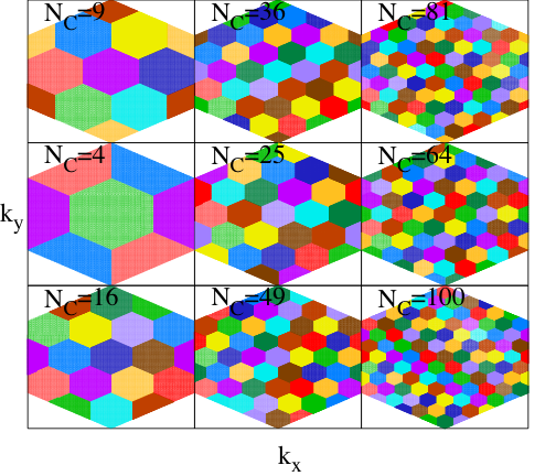
Figure 1: (Colour online) Dynamical cluster approximation (DCA) sub-zones for cluster sizes of up to $N_{C}=100$. The axes show the $x$- and $y$-components of the momentum, $k_{x}$ and $k_{y}$. Within each sub-zone, the self-energy is taken to be momentum independent. This allows Green functions to be calculated in the thermodynamic limit, and convergence properties are particularly good as $N_{C}$ is increased. Note that the only symmetry taken into account is translation in $\boldsymbol{k}$-space.

The electron-phonon Hamiltonian described above is extremely difficult to solve exactly using numerical methods. An approximate solution can be made using iterated perturbation theory within the dynamical cluster approximation formalism. The dynamical cluster approximation (DCA) hettler1998a ; hettler2000a is one of the possible ways of extending dynamical mean-field theory (DMFT)georges1996a so that it can be applied accurately to low dimensional systems. The Mermin-Wagner-Hohenberg theorem indicates that the significant non-local fluctuations found in some one- and two- dimensions could potentially lead to qualitatively incorrect results from mean-field theories mermin ; hohenberg . Moreover, DMFT has trouble dealing with the spatial variations involved with interactions that extend over more than one lattice site. DCA resolves this problem by developing a mean-field theory around a cluster, rather than a single site, therefore allowing the possibility of fluctuations or static spatial variations up to the length scale of the cluster.

When applying DCA, the Brillouin zone is divided up into $N_{C}$ sub-zones centered about a momentum vector $\boldsymbol{K}_{i}$ (see Fig. 1) consistent with the symmetry of the whole system. Within each sub-zone, the self-energy is approximated as a momentum-independent function, so the Green function can be coarse grained by integrating over the sub-zone,

$$\bf G\rm(\boldsymbol{K}_{i},z) = \sum_{\boldsymbol{k}\in\boldsymbol{K}_{i}}[\bf I\rm(z+\mu)+\Delta\boldsymbol{\sigma}_{3}-\boldsymbol{\Phi}_{\boldsymbol{k}}-\boldsymbol{\Sigma}(\boldsymbol{K}_{i},z)]^{-1}$$ (9)

$$\equiv \left[\begin{array}[]{cc}G_{AA}&G_{AB}\\ G_{BA}&G_{BB}\end{array}\right]$$ (12)

where A and B represent sublattices and

$$\boldsymbol{\Phi}_{\boldsymbol{k}}=\left[\begin{array}[]{cc}0&\phi_{\boldsymbol{k}}\\ \phi^{*}_{\boldsymbol{k}}&0\end{array}\right],\boldsymbol{\sigma}_{3}=\left[\begin{array}[]{cc}1&0\\ 0&-1\end{array}\right].$$ (13)

I will discuss the procedure for introducing long-range electron-phonon interactions in Sec. III.1.

In finite size techniques, the number of particles is related to the number of momentum points used in the calculation of the self energy. In contrast, the DCA coarse-graining step involves an infinite number of momentum points, so the thermodynamic limit is satisfied for any cluster size. In the context of the perturbation theory for the Migdal–Eliashberg theory used here, DCA has particularly good convergence properties in cluster size $N_{C}$, so in principle smaller clusters can be used leading to a significant improvement in computational efficiency hague2003a ; hague2005a . I note that when the DCA cluster size, $N_{C}=1$, calculations correspond to DMFT.

In several previous studies, $N_{C}=4$ and $N_{C}=16$ DCA clusters have been used to understand Hubbard interactions on hexagonal/triangular lattices (see e.g. lee2008a, ). I briefly discuss the subzone schemes for hexagonal lattices with larger $N_{C}$. For the lattices used here, the simplest way of defining the sub-zone vectors is: $\tilde{\boldsymbol{k}}_{1}=\boldsymbol{k}_{1}/\sqrt{N_{C}}$, $\tilde{\boldsymbol{k}}_{2}=\boldsymbol{k}_{2}/\sqrt{N_{C}}$ with the vectors $\boldsymbol{K}_{i}=n\tilde{\boldsymbol{k}}_{1}+m\tilde{\boldsymbol{k}}_{2}$ with $n$ and $m$ integers. Here, the reciprocal lattice vectors are $\boldsymbol{k}_{1}=(2\pi/3\tilde{a},2\pi/\sqrt{3}\tilde{a})$ and $\boldsymbol{k}_{2}=(2\pi/3\tilde{a},-2\pi/\sqrt{3}\tilde{a})$. There are likely to be other valid lattices that can also be used, where the lattice and sub-lattice are oriented at different angles. However, the lattices used there are the simplest to implement.

Even for the simple cases considered here, the resultant lattices can be ordered into groups. Clusters with $N_{C}=(3n)^{2}$ ($N_{C}=9$, $N_{C}=36$, $N_{C}=81$ etc.) have sub-zones centered on the K and K^′ points (here $n\geq 1$ is an integer). Those with $N_{c}=(3n-1)^{2}$ ($N_{C}=4$, $N_{C}=25$ and $N_{c}=64$) make a second set where 3 sub-zones share a corner at the K and K^′ points, and the third set of $N_{c}=(3n+1)^{2}$ ($N_{C}=16,64,100$ etc.) where 3 sub-zones share a corner at the K and K^′ points and an edge with the full Brillouin zone. Since the self energies would be identical in the 3 zones around the K and K^′ points in the latter 2 cases, they will poorly describe the physics at the K and K^′ points (which is especially important for graphene). This is why I use only the $(3n)^{2}$ series.

To establish which $\boldsymbol{k}$ point belongs to a sub zone, it is sufficient to find the closest $\boldsymbol{K}_{i}$ point corresponding to the center of the sub-zone (subject to shifts of reciprocal lattice vectors). The edges of the shapes defined in this way are the hexagons in the figure.

III.1 Self-consistent equations for the Fröhlich interaction

I now describe how the perturbation theory for the long-range electron-phonon interaction is used in conjunction with the DCA. The perturbation theory used here can be seen in Fig. 2. Panel (a) shows the Hartree diagram. For the symmetry broken states, this cannot be absorbed into the chemical potential, and is the main contributor to modification of the gap. The Fock diagram (shown in panel (b)) is responsible for frequency dependence of the self-energy. Phonon propagators are modified using a Dyson equation (panel (c)) which modifies the phonon frequency, and can lead to further enhancement of the band gap. Following the standard formulation of the DCA, where momentum is not conserved at vertices within the sub-zones (see e.g. Ref. maier2005a, for a good review), momentum sums in the perturbation theory are reduced to sums over the average momenta of the sub-zones. Therefore,

$$\Sigma^{(H)}_{XY}=-2\frac{T}{N_{C}}\delta_{XY}\sum_{lm\boldsymbol{K}^{\prime}}D_{Xl}(\boldsymbol{0})G_{ll}(\boldsymbol{K}^{\prime},\omega_{m})$$ (14)

$$\Sigma^{(F)}_{XY}(\omega_{n}\boldsymbol{K})=\frac{T}{N_{C}}\sum_{\omega_{s},\boldsymbol{Q}}G_{XY}(\omega_{n}-\omega_{s},\boldsymbol{K}-\boldsymbol{Q})D_{XY}(\omega_{s}\boldsymbol{Q})$$ (15)

where $\boldsymbol{Q}$ represent the centers of the coarse-grained cells for phonon momenta.

$$\left[D^{-1}(\boldsymbol{Q})\right]_{XY}=\left[d^{-1}(\boldsymbol{Q})\right]_{XY}-\left[\Pi(\boldsymbol{Q})\right]_{XY}$$ (16)

where

$$\Pi_{XY}(\boldsymbol{Q},\omega_{s})=-2\frac{T}{N_{C}}\sum_{\boldsymbol{K}\omega_{n}}G_{XY}(\boldsymbol{Q}+\boldsymbol{K},\omega_{n}+\omega_{s})G_{YX}(\boldsymbol{K},\omega_{n})$$ (17)

and the non-interacting phonon propagator is,

$$d_{XY}(\boldsymbol{Q},\omega_{s})=\lambda_{XY}(\boldsymbol{Q})\Omega^{2}/(\Omega^{2}+\omega_{s}^{2}).$$ (18)

where $\lambda_{XY}(\boldsymbol{Q})$ is the dimensionless electron phonon coupling averaged to a single sub-zone centered around momentum $\boldsymbol{Q}$.

It remains to define how to deal with the momentum dependent electron-phonon coupling within the DCA formalism. Here the dimensionless, momentum dependent electron-phonon coupling, $\lambda$, is incorporated using the following procedure. I first note that in position space, the standard dimensionless electron-phonon coupling is defined to be, $\lambda=\sum_{\boldsymbol{m}z}|g^{(z)}_{\boldsymbol{m}}(0)|^{2}/t\hbar\Omega$ (this value is the ratio of the polaron energy in the atomic limit to the hopping, $t$, see e.g. Ref. hague2007b, for more details), and that the Fourier transform of this definition to convert the sum to momentum space gives $\lambda=\sum_{\boldsymbol{k},XYz}|g^{(XY)}_{\boldsymbol{k},z}|^{2}/t\hbar\Omega$. Following this, I define the coupling for a single $\boldsymbol{k}$ and $z$ value to be,

$$\tilde{\lambda}^{(XY)}_{\boldsymbol{k},z}=|g^{(XY)}_{\boldsymbol{k},z}|^{2}/t\hbar\Omega$$ (19)

The dimensionless electron-phonon coupling can then be related to the value of $\lambda_{XY}(\boldsymbol{Q})$ used in equation 18 via,

$$\lambda_{XY}(\boldsymbol{K}_{i})=2N_{C}\lambda\frac{\sum_{\boldsymbol{k}\in\boldsymbol{K}_{i},z=1}^{z=N_{Z}}\tilde{\lambda}^{(XY)}_{\boldsymbol{k},z}}{\sum_{\boldsymbol{k}^{\prime}\in BZ,\alpha\beta,z=1}^{z=N_{Z}}\tilde{\lambda}^{(\alpha\beta)}_{\boldsymbol{k}^{\prime},z}}$$ (20)

where $N_{Z}$ is the number of planes of vibrating ions in the bulk substrate that electrons in the plane are coupled to (note that the electrons do not hop into the substrate). The reason for defining $\lambda_{XY}$ in this way is that it is a convenient way of cancelling the non-standard coupling constant, $\kappa$, and replacing it with the standard dimensionless electron-phonon coupling, $\lambda$. In this expression, the sum in the denominator leads to an average value that is proportional to $\lambda$ multiplied by the number of lattice sites, $2N_{C}$ (there are 2 sub-lattices for every cluster site), so by multiplying the average value of $\tilde{\lambda}_{\boldsymbol{k},z}$ in each DCA sub-zone by $2N_{C}\lambda/\sum_{\boldsymbol{k}^{\prime}\in BZ,nm,z}\tilde{\lambda}^{(nm)}_{\boldsymbol{k}^{\prime},z}$, factors of $\kappa$ cancel. To give an idea about how lambda varies for different DCA subzones, $\lambda_{XY}(\boldsymbol{K}_{i})$ is plotted in Fig. 3 for zones that are centered on the high symmetry directions.

Figure 2: Feynman diagrams showing the perturbation theory used in the work presented here. (a) Hartree diagram. For the symmetry broken states, this cannot be absorbed into the chemical potential, and is the main contributor to modification of the gap (b) The Fock potential is responsible for frequency dependence of the self-energy (c) Dyson equation for the phonon propagator. This renormalizes the phonon frequency, which can lead to further enhancement of the band gap.

Figure 3: Values of $\lambda_{XY}(\boldsymbol{K}_{i})$ plotted for zones that are centered on the high symmetry directions. The Fröhlich interaction used has an average $\lambda$ value of 1, so due to the inhomogeneity of the interaction across the Brillouin zone, the interaction in unit cells close to the $\Gamma$ point is larger than 1, and smaller than 1 elsewhere. The peak is supressed for small clusters due to averaging across DCA sub-zones, but reaches the peak value for cluster sizes of order 144. The difference between $\lambda_{AA}(\boldsymbol{K})$ and $\lambda_{AB}(\boldsymbol{K})$ at $\Gamma$ is important for the effective interaction strength in the Hartree diagram.

Self-consistency is then carried out as follows:

1. Initialise by calculating the coarse-grained electron-phonon interaction from Eqn. 20, and the Green function from Eqn. 9 with the electron self-energy set to zero.

2. Calculate the phonon self-energy (polarization bubble) from Eqn. 17

3. Calculate the renormalised phonon propagator from Eqn. 16.

4. Use the renormalized phonon propagator to calculate the Hartree and Fock contributions to the electron self-energy following Eqns. 14 and 15.

5. Re-calculate the Green function from Eqn. 9.

6. Repeat steps 2-5 until converged.

The resulting formalism is quite robust for phonon energies that are of the order of, or smaller than $kT$, as is the case with all calculations made here for room temperature and phonons with energies in the range $10-100$meV, since the phonon propagator acts like a $\delta$-function when $\hbar\Omega<k_{B}T$. Since the Hartree diagram does not have any frequency sums that include the phonon propagator, the sum over Matsubara frequencies in the next most important diagram (the Fock diagram) is severely truncated, leading to a much reduced contribution (with the caveat that the Green function must have small values for low Matsubara frequencies, which is ensured by the V-shaped form of the density of states in graphene). In practice, this means that all other terms in the perturbation expansion for the electron self-energy will be very much smaller, and that in this case (because of the vanishing DOS at the Fermi surface) Migdal’s theory holds. Similar considerations apply for the phonon self-energy such that the single polarisation bubble formed from dressed electron propagators should be the dominant term in the perturbation expansion. Therefore, the approximation used here is expected to be highly accurate for large cluster sizes.

III.2 Extensions for different interactions on A and B sublattices

Finally, I note that it is possible to have different electron-phonon interactions on each of the A and B sub-lattices. This may occur since atoms on the A and B sites are different, so that the orbitals holding the electrons that cause the ion displacements have a different form. In practice, I would expect this effect to be quite small ($\lesssim 30\%$) if A and B sites are in the same period of the periodic table, but this effect may be larger if the atoms come from different periods.

Starting again from the expression,

$$\tilde{\lambda}^{(XY)}_{\boldsymbol{k},z}=|g^{(XY)}_{\boldsymbol{k},z}|^{2}/t\hbar\Omega$$ (21)

Two dimensionless constants can now be introduced, $\lambda_{A}\propto\kappa_{A}^{2}$ and $\lambda_{B}\propto\kappa_{B}^{2}$. I note that the values of $|g^{(XY)}_{\boldsymbol{k},z}|^{2}$ are proportional to $\lambda_{A}$ if both sublattices are of type A, $\lambda_{B}$ if both sublattices are of type B, and $\sqrt{\lambda_{A}\lambda_{B}}$ if the sublattices are different. It is worth noting at this stage that the factor $\sqrt{\lambda_{A}\lambda_{B}}$ for off diagonal terms means that the inter-site interactions are reduced faster than the simple average of $\lambda_{A}$ and $\lambda_{B}$, which makes the interaction much more localized if the difference between $\lambda_{A}$ or $\lambda_{B}$ is significant.

The dimensionless electron-phonon coupling can then be related to the value of $\lambda_{XY}(\boldsymbol{Q})$ used in the self-consistent equations via,

$$\lambda_{XY}(\boldsymbol{K}_{i})=\frac{N_{C}}{2}(\sqrt{\lambda_{A}}+\sqrt{\lambda_{B}})^{2}\frac{\sum_{\boldsymbol{k}\in\boldsymbol{K}_{i},z}\tilde{\lambda}^{(XY)}_{\boldsymbol{k},z}}{\sum_{\boldsymbol{k}^{\prime}\in BZ,\alpha\beta,z}\tilde{\lambda}^{(\alpha\beta)}_{\boldsymbol{k}^{\prime},z}}$$ (22)

The prefactor in this expression is different to the previous one, since the sum in the denominator is proportional to $\lambda_{A}+\lambda_{B}+2\sqrt{\lambda_{A}\lambda_{B}}=(\sqrt{\lambda_{A}}+\sqrt{\lambda_{B}})^{2}$.

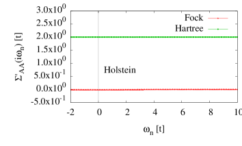
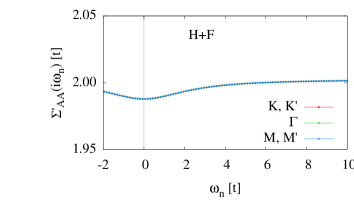
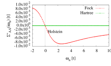
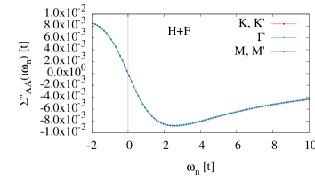
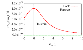
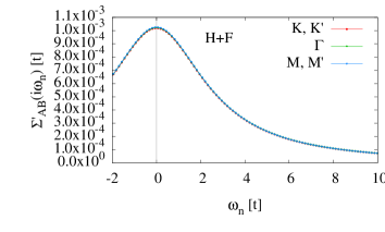
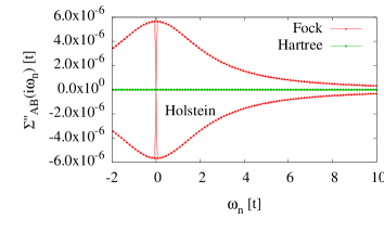
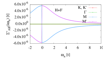
Figure 4: (color online) Comparison of Hartree and Fock parts of self energy for the case of the Holstein interaction, $\Sigma=\Sigma^{\prime}+i\Sigma^{\prime\prime}$ vs Matsubara frequency in a 9 site cluster. The largest element in the self energy matrix is the real part of the on-diagonal Hartree term, which is momentum independent, and it is this value that defines the size of the gap. Panels on the left show individual Hartree and Fock contributions to the gap and on the right show the momentum dependence of the total self energy. $\Sigma_{AA}$ is essentially momentum independent (so in the upper panel, curves for K and $\Gamma$ points lie directly under those for the M point), and $\Sigma_{AB}^{\prime}$ has weak momentum dependence, so the points can only be differentiated under high magnification. $\Sigma_{AB}^{\prime\prime}$ is very small. Primed points are related to unprimed ones by inversion around the origin. N.B. The Fock term is still the most important contribution in some cases, for example the inverse mass depends on derivatives of the self energy, so this will be given by the Fock term. The points marked M and M^′ represent zones that border on the M point (but where the DCA sub-zone center in the $N_{C}=9$ cluster is offset slightly from the M point so that the values can be distinct). $T=0.02t$, $\Delta=0.1t$, $\Omega=0.01t$ and $\lambda=2$.

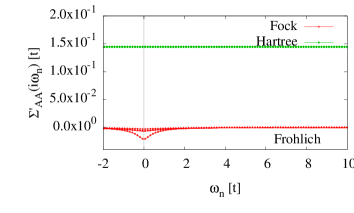
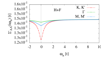
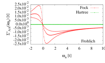
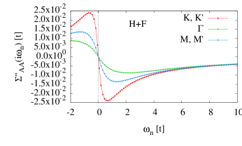
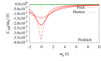
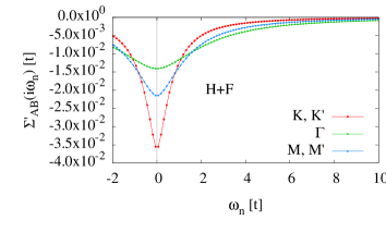
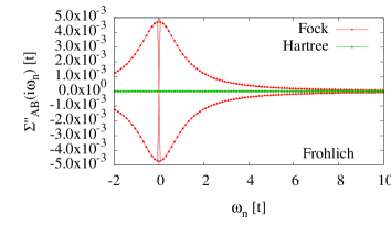
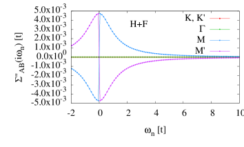
Figure 5: (color online) Comparison of Hartree and Fock parts of self energy for a Fröhlich interaction, $\Sigma=\Sigma^{\prime}+i\Sigma^{\prime\prime}$ vs Matsubara frequency. The on-diagonal contributions can be seen at the top and the off-diagonal ones at the bottom. Again, the largest contribution to the self energy matrix is the real part of the on-diagonal Hartree term, which defines the gap and is momentum independent. As in the Holstein case, the Hartree contibution to the off-diagonal self-energy is necessarily zero, and the Fock diagram is the largest off-diagonal contibution although it is still around 1/4 of the magnitude of the on-diagonal Hartree term. The Fock term has a significantly bigger momentum dependence than in the Holstein case. N.B. The contributions to $\Sigma_{AB}^{\prime\prime}$ for K, K^′ and $\Gamma$ points are all zero, so can not be distinguished from each other. Here, $T=0.02t$, $\Delta=0.1t$, $\Omega=0.01t$, $\lambda=2$ and $N_{C}=9$. The Fock contributions become relatively smaller compared to the Hartree term as cluster size increases.

IV Results

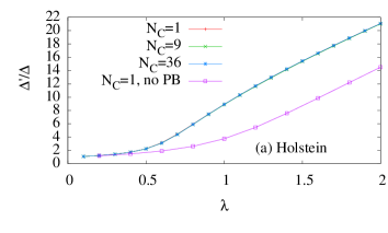
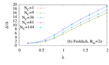
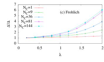
Figure 6: (color online) (a) Gap enhancement $\Delta^{\prime}/\Delta$ vs electron-phonon coupling $\lambda$ for a Holstein interaction with $\Delta/t=0.1$, comparing results from the dynamical mean-field theory (corresponding to $N_{C}=1$) and DCA. There are only small corrections due to momentum dependence. (b) Gap enhancement for the long range Fröhlich interaction, $R_{sc}=2a$ (c) Gap enhancement for the long range Fröhlich interaction. Here $T=0.02t$ and $\Omega=0.01t$. The initial increase in the gap as $N_{C}$ increases arises because the long range interaction is not homogenous across the Brillouin zone, so the effective value of $\lambda(\boldsymbol{Q}=0)$ (that is relevant to the Hartree diagram) is larger than the average $\lambda$ in all cluster sizes except $N_{C}=1$. The enhancement is essentially converged for cluster sizes of $N_{c}=144$. (N.B. Since $\Delta=0.1t$, the gap enhancement is 10 times larger than the gap, $\Delta^{\prime}$, which can be read from the real part of the self-energy at large Matsubara frequency.)

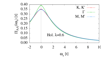
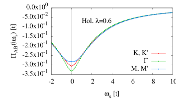
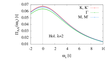
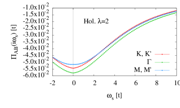
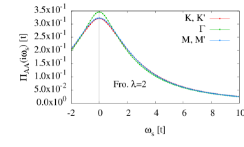
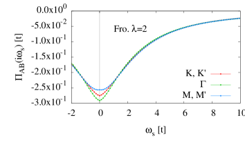
Figure 7: (color online) Comparisons of the phonon self energy for Holstein and Fröhlich interactions with various $\lambda$. As the interaction strength increases, the phonon self energy decreases due to the gap at the Fermi energy that reduces the value of the Green function at low Matsubara frequencies. The self energy is only weakly momentum dependent, but it is possible to discern the variation across the Brillouin zone.

Figure 8: Effective coupling in the Holstein model for a range of couplings, $D_{XY}(Q,0)$. The effective interaction becomes larger more rapidly than $\lambda$, and the form changes from momentum independent to weakly momentum dependent.

Figure 9: Effective coupling in the Fröhlich model for a range of couplings, $D_{ij}(Q,0)$. This property is strongly momentum dependent, and the momentum dependence becomes slightly larger as coupling increases. It is the effective coupling that leads to non-local position space variations that require large clusters to treat.

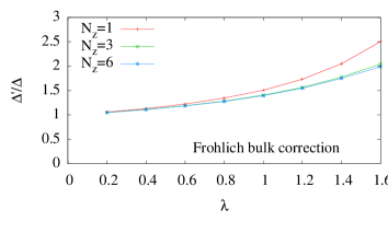
Figure 10: (color online) Corrections taking account of the finite depth of the bulk substrate. The traces show the effect of interactions between electrons in the monolayer and vibrations in the surface atoms only ($N_{z}=1$) and interactions with vibrations in 3 and 6 layers of bulk substrate respectively (N.B. electrons only hop in the monolayer, and there is no hopping into the bulk of the substrate). The effect of the bulk of the substrate is to reduce the enhanced gap by around 20%.

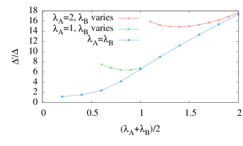
Figure 11: (color online) The effect of taking $\lambda_{A}\neq\lambda_{B}$ when $R_{sc}=2a$ and $N_{C}=36$. Since electrons on different sub-lattices are contained in orbitals of different atoms, the interaction between electrons and phonons may depend on the sub-lattice. The enhancement is mainly determined by the largest of $\lambda_{A}$ or $\lambda_{B}$ with small changes to the overall enhancement as the other coupling is varied.

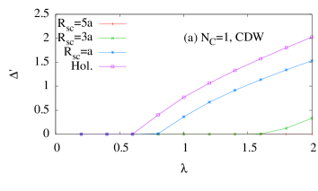
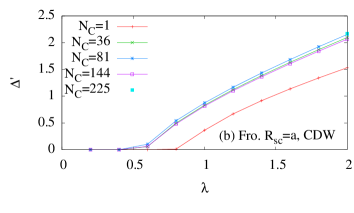
Figure 12: (color online) (a) Spontaneous symmetry breaking (gap generation) in a graphene monolayer. The $y$-axis shows the spontaneously formed gap, $\Delta^{\prime}$ and the $x$-axis the electron-phonon coupling $\lambda$. Here $T=0.02t$, $\Omega=0.01t$, $N_{C}=1$ and $\Delta=0$. (b) Effect of cluster size on the CDW state formed from a Fröhlich interaction with $R_{sc}=a$. N.B. A single point is calculated for cluster size of $N_{C}=225$ to confirm convergence.

The aim of the work presented here is to use dynamical cluster approximation (DCA) to examine how charge density wave (CDW) gaps in graphitic thin films vary with electron-phonon coupling. I take $T=0.02t$, $\Delta=0.1t$ and $\Omega=0.01t$. Noting that $t$ is typically on the order of an eV, these values correspond approximately to room temperature, phonon frequencies, $\Omega$, of 10s of meV and $\Delta$ a few hundred meV, consistent with thin films of materials such as InSb, or reported gaps in some graphene on substrate systems. In the following, all results are for half filling.

I start by computing self-energies to show the relative contributions of on- and off-site terms, and the effects of varying the interaction range. The computed self energies, including the relative contributions of Hartree and Fock diagrams for $\lambda=2$ and $N_{C}=9$ resulting from a Holstein interaction are shown in Fig. 4. The top two rows show real and imaginary parts of the on-diagonal self energy, and the bottom two rows show the off-diagonal self energy. The real part of the on-diagonal Hartree diagram is momentum and energy independent. It is the largest magnitude element of the self energy matrix (contribution around $2t$), and as it is frequency independent it directly contributes to the enhancement to the gap by changing the effective local potential on each sub-lattice, and it is also the main contributor to spontaneous CDW order. The imaginary part of the Hartree diagram and the off diagonal contributions are necessarily zero for the Holstein interaction. The imaginary part of the Fock term (contribution $\sim 0.1t$) is still the most important contribution for some properties. For example the inverse mass (not considered here) depends on derivatives of the self energy, so this property will be given by the Fock term. The Fock term is also the largest contribution to the off-diagonal self energy with a contribution of around $0.01t$. Note that when $\lambda_{A}=\lambda_{B}$, the self-energies have the following symmetries: $\Sigma_{BA}=\Sigma_{AB}^{*}$ and $\Sigma_{BB}=-\Sigma_{AA}^{*}$, so $\Sigma_{BA}$ and $\Sigma_{BB}$ are not shown.

Fig. 5 is as Fig. 4 for the longer ranged Fröhlich interaction (for $N_{C}=9$, the Hartree contribution is $0.15t$). The real parts of the on-site self energies are significantly smaller for the long-range Fröhlich interaction than for the Holstein model. Other differences are that the Fock contribution to the off-site self energy is very small for the Holstein interaction (N.B. it is not zero because of effective off-site interactions mediated through the phonon self-energy), whereas the off-site Fock self energy is of similar magnitude to (but smaller than) the onsite Fock self-energy for the Fröhlich interaction ($\sim 0.04t$). The relative size of the on-site Fock contribution drops off significantly relative to the Hartree diagram as cluster size is increased, only contributing $\sim 4\%$ of the total self energy at zero Matsubara frequency for $N_{C}=144$.

The main aim of this paper is to understand the role of electron-phonon coupling range in the enhancement of gaps. Figure 6 shows how the enhancement varies with interaction range and with cluster size. The gap size is calculated directly from the value of the Hartree diagram, which causes a local on-site potential energy shift, such that the gap, $\Delta^{\prime}\approx\Delta+\Sigma^{(H)}$, whereas the Fock term that contributes the imaginary on-site self-energy changes the quasi-particle lifetime. I have used Padé approximants vidberg to test for any further gap contribution from the Fock term, which is very small for the Holstein interaction, and for the Fröhlich interaction reduces from around 15% for a cluster of $N_{C}=9$ to around 2% for cluster size $N_{C}=144$. Figure 6(a) shows gap enhancement for a Holstein interaction with $\Delta/t=0.1$, for a range of cluster sizes. N.B. The enhancements will be smaller for systems with larger ionicity ($\Delta/t$) hague2011b ; hague2012a . There are very small corrections due to momentum dependence. As the screening radius, $R_{sc}$ increases, the enhancement decreases. Increase in cluster size has no effect on the gap in this set of diagrams for the Holstein interaction. Fig. 6(b) shows results when $R_{sc}=2a$. Essentially, the effective $\lambda$ (that goes like $\lambda_{AA}(0)-\lambda_{AB}(0)$ in the Hartree diagram) decreases with $R_{sc}$. The initial increase in the gap as $N_{C}$ is increased is a result of the inhomogeneity in the effective electron-phonon coupling across the Brillouin zone, which means that the value of coupling is largest at the $\Gamma$ point, where it contributes most to the Hartree diagram. For small clusters, averaging the coupling across the Brillouin zone means that the coupling is under-estimated at the zone center and over-estimated at the K point (see Fig. 3). Fig. 6(c) shows gap enhancement for the long range Fröhlich interaction ($R_{sc}\rightarrow\infty$). Even for the long range interaction, the enhancement effects are significant. I note that the DMFT results ($N_{C}=1$) consistently underestimate the gap enhancement.

The phonon self-energy plays an important role in the gap enhancement. Fig 6(a) also shows the enhancement effect for the Holstein interaction when $N_{C}=1$ if the polarization bubble (PB) is neglected and the curve can be compared with the full theory with $N_{C}=1$. The phonon self energy augments the enhancement by increasing the value of the phonon propagator at the Brillouin zone center. Thus, increasing the electron self-energy, which is proportional to the phonon propagator.

To show how the phonon self-energy varies within the Brillouin zone, it is plotted in Fig. 7. The variation is relatively small, which indicates that the position space variation occurs over a very small number of lattice sites, i.e. that only small clusters are needed to capture the spatial variation of $\Pi$. To show how the effective coupling is renormalised and depends on cluster size, $D(\boldsymbol{Q},0)$ is plotted in Figs. 8 and 9. The momentum dependence of the effective coupling when the Holstein interaction is used is very weak (Fig. 8). On the other hand, the effective coupling is strongly momentum dependent for the Fröhlich interaction. This demonstrates that it is the effective coupling causes the spatial variations that require large clusters to represent.

All results shown up to this point are calculated with electrons in the monolayer coupling to phonons in the surface layer of ions in the substrate only. Fig. 10 shows corrections taking account the finite depth of the bulk of the substrate rather than just surface ions. The plot shows the effect of including interaction with vibrations of surface ions only ($N_{z}=1$), and interaction with vibrations in 3 layers ($N_{z}=3$) and 6 layers ($N_{z}=6$) of the bulk of the substrate respectively (note that electrons still hop in the monolayer, and do not hop into the substrate). The effect of the bulk is to reduce the enhanced gap by around $20\%$.

Since the atoms on A and B sites may be different, their electron-phonon interactions may also be different. I test the effect of taking $\lambda_{A}\neq\lambda_{B}$, which is shown in Fig. 11. In the figure, $\lambda_{A}$ is kept fixed, while $\lambda_{B}$ is varied. The asymmetry induced between A and B sites by the interaction means that self-energies are not symmetric between A and B sites as before, so the chemical potential is varied iteratively during self consistency to maintain half filling. Curves computed for these parameters are compared with the enhancement when $\lambda_{A}=\lambda_{B}$, and the average value of $\lambda$ is plotted on the $x$-axis to make the comparison meaningful. As $\lambda_{B}$ is decreased, there is initially a small reduction in the enhancement of around 20%, followed by an increase as $\lambda_{B}$ approaches zero. For a comparable average $\lambda$, the enhancement is generally bigger than for the case when the two couplings are the same. The reason why the enhancement remains high is that large differences between the two couplings significantly reduce the coupling between A and B sites (which goes as $\sqrt{\lambda_{A}\lambda_{B}}$), and it is this coupling that acts to reduce the enhancement in the Hartree term.

While this paper is primarily concerned with the modification of gaps in graphene like (graphitic) materials with inherent ionicity, such as thin films of III-V semiconductors, it is also interesting to determine if gaps can spontaneously form from the electron-phonon interaction. This is explored in Fig. 12, which shows spontaneous charge density wave (CDW) symmetry breaking. Panel (a) shows DMFT results. For sufficient $\lambda$, a CDW state can be found for all values of $R_{sc}$ (this is not visible in the figure for large values of $R_{sc}$ because $\lambda$ values are too small). The result shows that the full system with $\Delta\neq 0$ is on the cusp of a CDW state, and this is why the gap is strongly sensitive to the electron-phonon coupling. Panel (b) shows results for $R_{sc}=1$ as the cluster size is increased. It may initially be of surprise that a CDW state can be supported at finite temperature, since Mermin-Wagner-Hohenberg (MWH) theorem does not allow for two dimensional antiferromagnetism in Heisenberg models or 2D superconductivity. However, detailed quantum Monte Carlo calculations have shown that CDW order can be formed by the Holstein interaction at half-filling on square lattices at finite temperature noack1991a ; vekic1992a ; niyaz1993a . In this case, MWH theorem does not apply because the symmetry is discrete (i.e. the local charge density at a specific time is determined by the number of electrons and may be 0, 1 or 2) nowadnick2012a .

To end this section, I note that as a minimum theory, it may be sufficient to compute only the Hartree diagram (which dominates the perturbation expansion) and the lowest order contribution to the phonon self energy, $\Pi$, at $\boldsymbol{Q}=0$ and $\omega_{s}=0$ only (since only the zero momentum Matsubara frequency and the phonon propagator contributes to the Hartree diagram). However, there would still need to be iteration over these diagrams to acheive self-consistency.

V Summary and conclusions

In summary, I have investigated gap formation and enhancement in a model of atomically thin graphitic materials. Electron-phonon coupling and range has been varied, and the effects of higher order corrections to the phonon propagator have been considered. The effect of reintroducing fluctuations around the mean field limit has also been investigated using the dynamical cluster approximation. Higher order corrections to the perturbation theory increase the gap enhancement. It is found that gaps are enhanced by electron-phonon interactions for all interaction ranges, with the enhancement decreasing as interaction range increases.

One of the driving factors of this enhancement is the proximity to a charge density wave state for a material without ionicity ($\Delta=0$) such as graphene. I have shown that sufficiently large coupling between electrons and phonons can lead to spontaneous CDW order. This instability to order shows why there are significant gap enhancements at large coupling when ionicity is introduced. The existance of CDW order at finite temperature in a 2D material such as graphene is consistent with detailed quantum Monte Carlo results for a square lattice noack1991a ; vekic1992a ; niyaz1993a ; nowadnick2012a and this could be stabilized further at room temperature with small interplane hopping of order 50meV (or around 1% of the in-plane hopping). Owing to the spontaneous symmetry breaking, an appropriately layered heterostructure of graphene and a wide gap insulating material such as BN might generate small spontaneous gaps of useful size due to CDW formation.

In experiments, the strength of the electron-phonon coupling could be varied in two ways. The first most obvious way to modify the coupling between substrate and film is to change the substrate. Highly ionic polarizable substrates would couple most strongly with the film, leading to the strongest effects. While the distance between graphene and substrate is of the order of 3Å, the force between free electrons and ions in a substrate (leading directly to electron-phonon coupling) would be large. In fact, dimensionless electron-phonon couplings of up to $\lambda=1$ have been reported in graphene on substrate systems from angle resolved photoemission spectroscopy studies (see Fig. 3 of Ref. siegel2012a, and references therein, note that much smaller interactions can be found with metal substrates where polarizability is low and coupling with the substrate is weak). An alternative way to dynamically decrease the electron-phonon interaction range and increase coupling strength would be to apply pressure to the film to move it closer to the substrate, which could be simpler to achieve experimentally than growing films on many different substrates.

I briefly mention that interactions with the vibrations of hydrogen (and other) atoms that are used to functionalize graphene to make graphane (and related materials) would be Holstein like, so part of the gap in those materials may be phonon driven. This might be testable by changing the isotope of the functionalizing atoms.

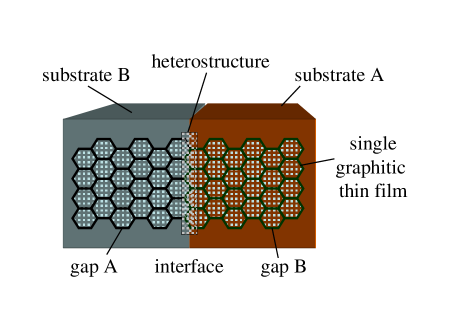
Figure 13: Schematic showing the possible use of two substrates with different electron-phonon coupling, $\lambda$ to thin graphitic films to make a heterostructure in a single thin film of a graphitic material. This could be manufactured by laying down an interface between the two substrate materials before cleaving perpendicular to the interface and then depositing the thin film. The film above the substrate with the largest $\lambda$ would have a bigger gap, leading to a heterostructure within the interface region.

The results here suggest that an interesting possibility would be to use the electron-phonon interaction to make position dependent changes to the bandstructure of the thin film (for example by adding a spatially dependent superstrate with phonons that strongly couple to electrons in the thin film), a method that is potentially easier to control than trying to deposit neighboring thin films with interfaces in the plane. Only tiny gap enhancements of around 20% would be needed so that proportional gap enhancements from the predictions made here are similar to the proportional difference between gaps in GaAs and AlGaAs ando1982a , so it is plausible that thin film heterostructures or quantum dots could be built up in this way (see Fig. 13). Another possibility would be to tune inherent gaps in III-V semiconductors with the electron-phonon interaction, so that they become optimal for applications such as solar cells where the efficiency is highly sensitive to the gap size. Clearly graphitic thin films warrant further study to assess their full capability for novel electronics.

References

- [1] K.S. Novoselov, D. Jiang, F. Schedin, T. J. Booth, V. V. Khotkevich, S. V. Morozov, and A. K. Geim. PNAS, 102:10453, 2005.
- [2] L. Song, L. Ci, H. Lu, P.B. Sorokin, C. Jin, J. Ni, A.G. Kvashnin, D.G. Kvashnin, J. Lou, B.I. Yakobson, and P.M. Ajayan. Nano Lett., 10:3209, 2010.
- [3] J. Wu, W. Walukiewicz, K.M. Yu, J.W. Ager, E.E. Haller, H. Lu, W.J. Schaff, Y. Saito, and Y. Nanishi. App. Phys. Lett., 80:3967, 2002.
- [4] I.H. Khan. Surface Science, 9:306, 1968.
- [5] R.K. Bedi and S. Kaur T. Singh. Thin Solid Films, 298:47, 1997.
- [6] J. Petalas, S. Logothetidis, S. Boultadakis, M. Alouani, and J.M. Wills. Phys. Rev. B, 52:8082, 1995.
- [7] F. Litimein, B. Bouhafs, Z. Dridi, and P. Ruterana. New J. Phys., 4:64, 2002.
- [8] C. Enderlein, Y. S. Kim, A. Bostwick, E. Rotenberg, and K. Horn. New J. Phys., 12:033014, 2010.
- [9] S. Y. Zhou, G.-H. Gweon, A. V. Fedorov, P. N. First, W. A. De Heer, D.-H. Lee, F. Guinea, A. H. Castro Neto, and A. Lanzara. Nature Materials, 6:770, 2007.
- [10] A. Bostwick, T. Ohta, T. Seyller, K. Horn, and E. Rotenberg. Nature Physics, 3:36, 2007.
- [11] S. Tongay, J. Zhou, C. Ataca, K. Lo, T.S. Matthews, J. Li, J.C. Grossman, and Junqiao Wu. Nano Lett., 12:5576, 2012.
- [12] J. P. Hague. Phys. Rev. B, 84:155438, 2011.
- [13] J. P. Hague. Nanoscale research letters, 7:303, 2012.
- [14] J.P. Hague. Phys. Rev. B, 86:064302, 2012.
- [15] A. S. Alexandrov and P. E. Kornilovitch. J. Phys.: Condens. Matter, 14:5337, 2002.
- [16] D.A.Siegel, C.Hwang, A.V.Fedorov, and A.Lanzara. New Journal of Physics, 14:095006, 2012.
- [17] There are two electron-phonon couplings in graphene, one between electrons in the plane and phonons in the plane, and another between electrons in the plane and phonons in the substrate. Coupling between electrons and in-plane phonons vanishes at half filling, as is the case for graphene on metals where weak coupling is expected with the substrate, whereas the electron-phonon interaction measured for graphene on SiC has no significant doping dependence, indicative that the coupling is with the substrate. In most cases, the coupling measured with ARPES is several times higher than would be expected if there were no coupling to the substrate.
- [18] A. Grüneis, C. Attaccalite, A. Rubio, D. Vyalikh, S.L. Molodtsov, J. Fink, R. Follath, W. Eberhardt, B. Büchner, and T. Pichler. Phys. Rev. B, 79:205106, 2009.
- [19] M. Calandra and F. Mauri. Phys. Rev. B, 76:205411, 2007.
- [20] W.K. Tse and S. Das Sarma. Phys. Rev. Lett., 99:236802, 2007.
- [21] C.H. Park, F. Giustino, M.L. Cohen, and S.G. Louie. Nano letters, 8:4229, 2008.
- [22] A. H. Castro Neto, F. Guinea, N. M. R. Peres, K. S. Novoselov, and A. K. Geim. Rev. Mod. Phys., 81:109, 2009.
- [23] E. McCann and V. I. Fal’ko. Phys. Rev. Lett., 96:086805, 2006.
- [24] E. McCann, D. S. L. Abergel, and V. I. Falko. Solid State Communications, 143:110, 2007.
- [25] T. Ohta, A. Bostwick, T. Seyller, K. Horn, and E. Rotenberg. Science, 313:951, 2006.
- [26] Y. Zhang, T-T. Tang, C. Girit, Z. Hao, M. C. Martin, A. Zettl, M. F. Crommie, Y. R. Shen, and F. Wang. Nature, 459:820, 2009.
- [27] M. Y. Han, B. Özyilmaz, Y. Zhang, and P. Kim. Phys. Rev. Lett., 98:206805, 2007.
- [28] D. V. Kosynkin, A. L. Higginbotham, A. Sinitskii, J. R. Lomeda, A. Dimiev, B. K. Price, and J. M. Tour. Nature, 458:872, 2009.
- [29] J. Hicks, A. Tejeda, A. Taleb-Ibrahimi, M. S. Nevius, F. Wang, K. Shepperd, J. Palmer, F. Bertran, P. Le Fèvre, J. Kunc, W. A. de Heer, C. Berger, and E. H. Conrad. Nat. Phys., 9:49, 2012.
- [30] Jorge O. Sofo, Ajay S. Chaudhari, and Greg D. Barber. Graphane: A two-dimensional hydrocarbon. Phys. Rev. B, 75:153401, Apr 2007.
- [31] D. W. Boukhvalov, M. I. Katsnelson, and A. I. lichtenstein. Phys. Rev. B, 77:035427, 2008.
- [32] D. C. Elias, R. R. Nair, T. M. G. Mohiuddin, S. V. Morozov, P. Blake, M. P. Halsall, A. C. Ferrari, D. W. Boukhvalov, M. I. Katsnelson, A. K. Geim, and K. S. Novoselov. Science, 323:610, 2009.
- [33] J.-C. Charlier, X. Gonze, and J.-P. Michenaud. First-principles study of graphite monofluoride (cf. Phys. Rev. B, 47:16162–16168, Jun 1993.
- [34] S.-H. Cheng, K. Zou, F. Okino, H. R. Gutierrez, A. Gupta, N. Shen, P. C. Eklund, J. O. Sofo, and J. Zhu. Reversible fluorination of graphene: Evidence of a two-dimensional wide bandgap semiconductor. Phys. Rev. B, 81:205435, May 2010.
- [35] J. Serrano, A. Bosak, R. Arenal, M. Krisch, K. Watanabe, T. Taniguchi, H. Kanda, A. Rubio, and L. Wirtz. Phys. Rev. Lett., 98:095503, 2007.
- [36] M. Steiner, M. Freitag, V. Perebeinos, J. C. Tsang, J. P. Small, M. Kinoshita, D. Yuan, J. Liu, and P. Avouris. Nature Nanotechnology, 4:320, 2009.
- [37] T. Holstein. Ann. Phys., NY, 8:325, 1959.
- [38] N. Nagaosa and J. Takimoto. J. Phys. Soc. Jpn., 55:2735, 1986.
- [39] M. Hettler, A.N. Tahvildar-Zadeh, M. Jarrell, Th. Pruschke, and H.R. Krishnamurthy. Phys. Rev. B, 58:7475, 1998.
- [40] M. Hettler, M. Mukherjee, M. Jarrell, and H.R. Krishnamurthy. Phys. Rev. B, 61:12739, 2000.
- [41] Where DMFT is used to approximate low dimensional systems, it is often known as the local approximation.
- [42] A. Georges, G. Kotliar, W. Krauth, and M. Rozenburg M. Rev. Mod. Phys, 68:13, 1996.
- [43] N.D. Mermin and H. Wagner. Phys. Rev. Lett., 17:1133, 1966.
- [44] P.C. Hohenberg. Phys. Rev., 158:383, 1967.
- [45] J.P. Hague. J. Phys.: Condens. Matter, 15:2535, 2003.
- [46] J.P. Hague. J. Phys.: Condens. Matter, 17:5663, 2005.
- [47] H. Lee, G. Li, and H. Monien. Phys. Rev. B, 78:205117, 2008.
- [48] T. Maier, M. Jarrell, T. Pruschke, and M. H. Hettler. Rev. Mod. Phys., 77:1027, 2005.
- [49] J.P. Hague, P.E. Kornilovitch, J.H. Samson, and A.S. Alexandrov. J. Phys.: Condens. Matter, 19:255214, 2007.
- [50] H.J. Vidberg and J.W. Serene. J. Low Temp. Phys., 29:179, 1977.
- [51] R.M. Noack, D.J. Scalapino, and R.T. Scalettar. Phys. Rev. Lett., 66:778, 1991.
- [52] M. Vekić, R.M. Noack, and S.R. White. Phys. Rev. B, 46:271, 1992.
- [53] P. Niyaz, J.E. Gubernatis, R.T. Scalettar, and C.Y. Fong. Phys. Rev. B, 48:16011, 1993.
- [54] E.A. Nowadnick, S. Johnston, B. Moritz, R.T. Scalettar, and T.P. Devereaux. Phys. Rev. Lett., 109:246404, 2012.
- [55] Tsuneya Ando, Alan B. Fowler, and Frank Stern. Rev. Mod. Phys., 54:437, 1982.