Expectation Propagation for Neural Networks with Sparsity-promoting Priors

Abstract

We propose a novel approach for nonlinear regression using a two-layer neural network (NN) model structure with sparsity-favoring hierarchical priors on the network weights. We present an expectation propagation (EP) approach for approximate integration over the posterior distribution of the weights, the hierarchical scale parameters of the priors, and the residual scale. Using a factorized posterior approximation we derive a computationally efficient algorithm, whose complexity scales similarly to an ensemble of independent sparse linear models. The approach enables flexible definition of weight priors with different sparseness properties such as independent Laplace priors with a common scale parameter or Gaussian automatic relevance determination (ARD) priors with different relevance parameters for all inputs. The approach can be extended beyond standard activation functions and NN model structures to form flexible nonlinear predictors from multiple sparse linear models. The effects of the hierarchical priors and the predictive performance of the algorithm are assessed using both simulated and real-world data. Comparisons are made to two alternative models with ARD priors: a Gaussian process with a NN covariance function and marginal maximum a posteriori estimates of the relevance parameters, and a NN with Markov chain Monte Carlo integration over all the unknown model parameters.

Keywords: expectation propagation, neural network, multilayer perceptron, linear model, sparse prior, automatic relevance determination

1 Introduction

Gaussian priors may not be the best possible choice for the input layer weights of a feedforward neural network (NN) because allowing, a priori, a large weight $w_{j}$ for a potentially irrelevant feature $x_{j}$ may deteriorate the predictive performance. This behavior is analogous to a linear model because the input layer weights associated with each hidden unit of a multilayer perceptron (MLP) network can be interpreted as separate linear models whose outputs are combined nonlinearly in the next layer. Integrating over the posterior uncertainty of the unknown input weights mitigates the potentially harmful effects of irrelevant features but it may not be sufficient if the number of input features, or the total number of unknown variables, grows large compared with the number of observations. In such cases, an alternative strategy is required to suppress the effect of the irrelevant features. In this article we focus on a two-layer MLP model structure but aim to form a more general framework that can be used to combine linear models with sparsity-promoting priors using general activation functions and interaction terms between the hidden units.

A popular approach has been to apply hierarchical automatic relevance determination (ARD) priors (Mackay, 1995; Neal, 1996), where individual Gaussian priors are assigned for each weight, $w_{j}\sim\mathcal{N}(0,\alpha_{l_{j}})$, with separate variance hyperparameters $\alpha_{l_{j}}$ controlling the relevance of the group of weights related to each feature. Mackay (1995) described an ARD approach for NNs, where point estimates for the relevance parameters $\alpha_{l_{j}}$ along with other model hyperparameters, such as the noise level, are determined using a marginal likelihood estimate obtained by approximate integration over the weights with Laplace’s method. Neal (1996) proposed an alternative Markov chain Monte Carlo (MCMC) approach, where approximate integration is performed over the posterior uncertainty of all the model parameters including $w_{j}$ and $\alpha_{l_{j}}$. In connection with linear models, various computationally more efficient algorithms have been proposed for determining marginal likelihood based point estimates for the relevance parameters (Tipping, 2001; Qi et al., 2004; Wipf and Nagarajan, 2008). The point-estimate based methods, however, may suffer from overfitting because the maximum a posteriori (MAP) estimate of $\alpha_{l_{j}}$ may be close to zero also for relevant features as demonstrated by Qi et al. (2004). The same applies also for infinite neural networks implemented using Gaussian process (GP) priors when separate hyperparameters controlling the nonlinearity of each input are optimized (Williams, 1998; Rasmussen and Williams, 2006).

Recently, appealing surrogates for ARD priors have been presented for linear models. These approaches are based on sparsity favoring priors, such as the Laplace prior (Seeger, 2008) and the spike and slab prior (Hernández-Lobato et al., 2008, 2010). The methods utilize the expectation propagation (EP) (Minka, 2001a) algorithm to efficiently integrate over the analytically intractable posterior distributions. Importantly, these sparse priors do not suffer from similar overfitting as many ARD approaches because point estimates of feature specific parameters such as $\alpha_{l_{j}}$ are not used, but instead, approximate integration is done over the posterior uncertainty resulting from a sparse prior on the weights. Expectation propagation provides a useful alternative to MCMC for carrying out the approximate integration because it has been found computationally efficient and very accurate in many practical applications (Nickisch and Rasmussen, 2008; Hernández-Lobato et al., 2010).

In nonlinear regression, sparsity favoring Laplace priors have been considered for NNs, for instance, by Williams (1995), where the inference is performed using the Laplace approximation. However, a problem with the Laplace approximation is that the curvature of the log-posterior density at the posterior mode may not be well defined for all types of prior distributions, such as, the Laplace distribution whose derivatives are not continuous at the origin (Williams, 1995; Seeger, 2008). Implementing a successful algorithm requires some additional approximations as described by Williams (1995), whereas with EP the implementation is straightforward since it relies only on expectations of the prior terms with respect to a Gaussian measure.

Another possibly undesired characteristic of the Laplace approximation is that it approximates the posterior mean of the unknowns with their MAP estimate and their posterior covariance with the negative Hessian of the posterior distribution at the mode. This local estimate may not represent well the overall uncertainty on the unknown variables and it may lead to worse predictive performance for example when the posterior distribution is skewed (Nickisch and Rasmussen, 2008) or multimodal (Jylänki et al., 2011). Furthermore, when there are many unknowns compared to the effective number of observations, which is typical in practical NN applications, the MAP solution may differ significantly from the posterior mean. For example, with linear models the Laplace prior leads to strictly sparse estimates with many zero weight values only when the MAP estimator of the weights is used. The posterior mean estimate, on the other hand, can result in many clearly nonzero values for the same weights whose MAP estimates are zero (Seeger, 2008). In such case the Laplace approximation underestimates the uncertainty of the feature relevances, that is, the joint mode is sharply peaked at zero but the bulk of the probability mass is distributed widely at nonzero weight values. Recently, it has also been shown that in connection with linear models the ARD solution is exactly equivalent to a MAP estimate of the coefficients obtained using a particular class of non-factorized coefficient prior distributions which includes models that have desirable advantages over MAP weight estimates (Wipf and Nagarajan, 2008; Wipf et al., 2011). This connection suggests that the Laplace approximation of the input weights with a sparse prior may possess more similar characteristics with the point-estimate based ARD solution compared to the posterior mean solution.

Our aim is to introduce the benefits of the sparse linear models (Seeger, 2008; Hernández-Lobato et al., 2008) into nonlinear regression by combining the sparse priors with a two-layer NN in a computationally efficient EP framework. We propose a logical extension of the linear regression models by adopting the algorithms presented for sparse linear models to MLPs with a linear input layer. For this purpose, the main challenge is constructing a reliable Gaussian EP approximation for the analytically intractable likelihood resulting from the NN observation model. Previously, Gaussian approximations for NN models have been formed using the extended Kalman filter (EKF) (de Freitas, 1999) and the unscented Kalman filter (UKF) (Wan and van der Merwe, 2000). Alternative mean field approaches possessing similar characteristic with EP have been proposed by Opper and Winther (1996) and Winther (2001).

We extend the ideas from the UKF approach by utilizing similar decoupling approximations for the weights as proposed by Puskorius and Feldkamp (1991) for EKF-based inference and derive a computationally efficient algorithm that does not require numerical sigma point approximations for multi-dimensional integrals. We propose a posterior approximation that assumes the weights associated with the output-layer and each hidden unit independent. The complexity of the EP updates in the resulting algorithm scale linearly with respect to the number of hidden units and they require only one-dimensional numerical quadratures. The complexity of the posterior computations scale similarly to an ensemble of independent sparse linear models (one for each hidden unit) with one additional linear predictor associated with the output layer. It follows that all existing methodology on sparse linear models (e.g., methods that facilitate computations with large number of inputs) can be applied separately on the sparse linear model corresponding to each hidden unit. Furthermore, the complexity of the algorithm scales linearly with respect to the number of observations, which is beneficial for large datasets. The proposed approach can also be extended beyond standard activation functions and NN model structures, for example, by including a linear hidden unit or predefined interactions between the linear input-layer models.

In addition to generalizing the standard EP framework for sparse linear models we introduce an efficient EP approach for inference on the unknown hyperparameters, such as the noise level and the scale parameters of the weight priors. This framework enables flexible definition of different hierarchical priors, such as one common scale parameter for all input weights, or a separate scale parameter for all weights associated with one input variable (i.e., an integrated ARD prior). For example, assigning independent Laplace priors on the input weights with a common unknown scale parameter does not produce very sparse approximate posterior mean solutions, but, if required, more sparse solutions can be obtained by adjusting the common hyperprior of the scale parameters with the ARD specification. We show that by making independent approximations for the hyperparameters, the inference on them can be done simultaneously within the EP algorithm for the network weights, without the need for separate optimization steps which is common for many EP approaches for sparse linear models and GPs (Rasmussen and Williams, 2006; Seeger, 2008), as well as combined EKF and expectation maximization (EM) algorithms for NNs (de Freitas, 1999). Additional benefits are achieved by introducing left-truncated priors on the output weights which prevent possible convergence problems in the EP algorithm resulting from inherent unidentifiability in the MLP network specification.

The main contributions of the paper can be summarized as:

• An efficiently scaling EP approximation for the non-Gaussian likelihood resulting from the MLP-model that requires numerical approximations only for one-dimensional integrals. We derive closed-form solutions for the parameters of the site term approximations, which can be interpreted as pseudo-observations of a linear model associated with each hidden unit (Sections 3.1–3.3 and Appendices A–E).

• An EP approach for integrating over the posterior uncertainty of the input weights and their hierarchical scale parameters assigned on predefined weight groups (Sections 3.1 and 3.2.1). The approach could be applied also for sparse linear models to construct factorized approximations for predefined weight groups with shared hyperparameters.

• Approximate integration over the posterior uncertainty of the observation noise simultaneously within the EP algorithm for inference on the weights of a MLP-network (see Appendix D). Using factorizing approximations, the approach could be extended also for approximate inference on other hyperparameters associated with the likelihood terms and could be applied, for example, in recursive filtering.

Key properties of the proposed model are first demonstrated with three artificial case studies in which comparisons are made with a neural network with infinitely many hidden units implemented as a GP regression model with a NN covariance function and an ARD prior (Williams, 1998; Rasmussen and Williams, 2006). Finally, the predictive performance of the proposed approach is assessed using four real-world data sets and comparisons are made with two alternative models with ARD priors: a GP with a NN covariance function where point estimates of the relevance hyperparameters are determined by optimizing their marginal posterior distribution, and a NN where approximate inference on all unknowns is done using MCMC (Neal, 1996).

2 The Model

We focus on two layer NNs where the unknown function value $f_{i}=f(\mathbf{x}_{i})$ related to a $d$-dimensional input vector $\mathbf{x}_{i}$ is modeled as

$$f(\mathbf{x}_{i})=\sum_{k=1}^{K}v_{k}g(\mathbf{w}_{k}^{\text{T}}\mathbf{x}_{i})+v_{0},$$ (1)

where $g(x)$ is a nonlinear activation function, $K$ the number of hidden units, and $v_{0}$ the output bias. Vector $\mathbf{w}_{k}=[w_{k,1},w_{k,2},...,w_{k,d}]^{\text{T}}$ contains the input layer weights related to hidden unit $k$ and $v_{k}$ is the corresponding output layer weight. Input biases can be introduced by adding a constant term to the input vectors $\mathbf{x}_{k}$. In the sequel, all weights are denoted by vector $\mathbf{z}=[\mathbf{w}^{\text{T}},\mathbf{v}^{\text{T}}]^{\text{T}}$, where $\mathbf{w}=[\mathbf{w}_{1}^{\text{T}},...,\mathbf{w}_{K}^{\text{T}}]^{\text{T}}$, and $\mathbf{v}=[v_{1},...,v_{K},v_{0}]^{\text{T}}$.

In this work, we use the following activation function:

$$g(x)=\frac{1}{\sqrt{K}}\operatorname{erf}\left(\frac{x}{\sqrt{2}}\right)=\frac{2}{\sqrt{K}}\left(\Phi(x)-0.5\right),$$ (2)

where $\Phi(x)=\int_{-\infty}^{x}\mathcal{N}(t|0,1)dt$, and the scaling by $1/\sqrt{K}$ ensures that the prior variance of $f(\mathbf{x}_{i})$ does not increase with $K$ assuming fixed Gaussian priors on $v_{k}$ and $w_{kj}$. We focus on regression problems with Gaussian observation model $p(y_{i}|f_{i},\sigma^{2})=\mathcal{N}(y_{i}|f_{i},\sigma^{2})$, where $\sigma^{2}$ is the noise variance. However, the proposed approach could be extended for other activation functions and observations models, for example, the probit model for binary classification.

2.1 Prior Definitions

To reduce the effects of irrelevant features, independent zero-mean Laplace priors are assigned for the input layer weights:

$$p(w_{j}|\lambda_{l_{j}})=\frac{1}{2\lambda_{l_{j}}}\exp\left(-\frac{1}{\lambda_{l_{j}}}|w_{j}|\right),$$ (3)

where $w_{j}$ is the $j$:th element of $\mathbf{w}$, and $\lambda_{l_{j}}=2^{-1/2}\exp(\phi_{l_{j}}/2)$ is a joint hyperparameter controlling the prior variance of all input weights belonging to group $l_{j}\in\{1,...,L\}$, that is, $\operatorname{Var}(w_{j}|\lambda_{l_{j}})=2\lambda_{l_{j}}^{2}$. Here index variable $l_{j}$ defines the group in which the weight $\mathbf{w}_{j}$ belongs to. The EP approximate inference is done using the transformed scale parameters $\phi_{l}=\log(2\lambda_{l}^{2})\in\mathbb{R}$. The grouping of the weights can be chosen freely and also other weight prior distributions can be used in place of the Laplace distribution (3). By defining a suitable prior on the unknown group scales $\phi_{l}$ useful hierarchical priors can be implemented on the input layer. Possible definitions include one common scale parameter for all inputs ($L=1$), and a separate scale parameter for all weights related to each feature, which implements an ARD prior ($L=d$). To obtain the traditional ARD setting the Laplace priors (3) can be replaced with Gaussian distributions $p(w_{j}|\lambda_{l_{j}})=\mathcal{N}(w_{j}|0,\exp(\phi_{l_{j}}))$. When the scale parameters $\{\phi_{l}\}_{l=1}^{L}$ are considered unknown, Gaussian hyperpriors are assigned to them:

$$\phi_{l}=\log(2\lambda_{l}^{2})\sim\mathcal{N}(\mu_{\phi,0},\sigma_{\phi,0}^{2}),$$ (4)

where a common mean $\mu_{\phi,0}$ and variance $\sigma_{\phi,0}^{2}$ have been defined for all groups $l=1,...,L$. Definition (4) corresponds to a log-normal prior on the associated prior variance $2\lambda_{l}^{2}=\exp(\phi_{l})$ for the weights in group $l$.

Because of the symmetry $g(x)=-g(-x)$ of the activation function, changing the signs of output weight $v_{k}$ and the corresponding input weights $\mathbf{w}_{k}$ results in the same prediction $f(\mathbf{x})$. This unidentifiability may cause converge problems in the EP algorithm: if the approximate posterior probability mass of output weight $v_{k}$ concentrates too close to zero, expected values of $v_{k}$ and $\mathbf{w}_{k}$ may start fluctuating between small positive and negative values. Therefore the output weights are constrained to positive values by assigning left-truncated heavy-tailed priors to them:

$$p(v_{k}|\sigma_{v,0}^{2})=2t_{\nu}(v_{k}|0,\sigma_{v,0}^{2}),$$ (5)

where $v_{k}\geq 0$, $k=1,...,K$, and $t_{\nu}(v_{k}|0,\sigma_{v,0}^{2})$ denotes a Student-$t$ distribution with degrees of freedom $\nu$, mean zero, and scale parameter $\sigma_{v,0}^{2}$. The prior scale is fixed to $\sigma_{v,0}^{2}=1$ and the degrees of freedom to $\nu=4$, which by experiments was found to produce sufficiently large posterior variations of $f(\mathbf{x})$ when the activation function is scaled according to (2) and the observations are normalized to zero mean and unit variance. The heavy-tailed prior (5) enables very large output weights if required, for example, when some hidden unit is forming almost a linear predictor (see, e.g, Section 4.2). A zero-mean Gaussian prior is assigned to the output bias: $p(v_{0}|\sigma_{v_{0},0}^{2})=\mathcal{N}(0,\sigma_{v_{0},0}^{2})$, where the scale parameter is fixed to $\sigma_{v_{0},0}^{2}=1$ because it was also found to be a sufficient simplification with the same data normalization conditions. The noise level $\sigma^{2}$ is assumed unknown and therefore a log-normal prior is assigned to it:

$$\theta=\log(\sigma^{2})\sim\mathcal{N}(\mu_{\theta,0},\sigma_{\theta,0}^{2})$$ (6)

with prior mean $\mu_{\theta,0}$ and variance $\sigma_{\theta,0}^{2}$.

The values of the hyperparameters $\lambda_{l}=2^{-1/2}\exp(\phi_{l}/2)$ and $\sigma_{v,0}^{2}$ affect the smoothness properties of the model in different ways. In the following discussion we first assume that there is only one input scale parameter $\lambda_{l}$ ($L=1$) for clarity. Choosing a smaller value for $\lambda_{l}$ penalizes more strongly for larger input weights and produces smoother functions with respect to changes in the input features. More precisely, in the two-layer NN model (1) the magnitudes of the input weights (or equivalently the ARD scale parameters) are related to the nonlinearity of the latent function $f(\mathbf{x})$ with respect to the corresponding inputs $\mathbf{x}$. Strong nonlinearities require large input weights whereas almost a linear function is obtained with a very large output weight and very small input weights for a certain hidden unit (see Section 4.2 for illustration).

Because the values of the activation function $g(x)$ are constrained to the interval $[-1,1]$, hyperparameter $\sigma_{v,0}^{2}$ controls the overall magnitude of the latent function $f(\mathbf{x})$. Larger values of $\sigma_{v,0}^{2}$ increase the magnitude of the steps the hidden unit activation $v_{k}g(\mathbf{w}_{k}^{\text{T}}\mathbf{x})$ can take in the direction of weight vector $\mathbf{w}_{k}$ in the feature space. Choosing a smaller value for $\sigma_{v,0}^{2}$ can improve the predictive performance by constraining the overall flexibility of the model but too small value can prevent the model from explaining all the variance in the target variable $y$. In this work, we keep $\sigma_{v,0}^{2}$ fixed to a sufficiently large value and infer $\lambda_{l}$ from data promoting simultaneously smoother solutions with the prior on $\phi_{l}=\log(2\lambda_{l}^{2})$. If only one common scale parameter $\phi_{l}$ is used, the sparsity-inducing properties of the prior depend on the shape of the joint distribution $p(\mathbf{w}|\bm{\lambda})=\prod_{j}p(w_{j}|\lambda_{l})$ resulting from the choice of the prior terms (3). By decreasing $\mu_{\phi,0}$, we can favor smaller input weight values overall, and with $\sigma_{\phi,0}^{2}$, we can adjust the thickness of the tails of $p(\mathbf{w}|\bm{\lambda})$. On the other hand, if individual scale parameters are assigned for all inputs according to the ARD setting, a family of sparsity-promoting priors is obtained by adjusting $\mu_{\phi,0}$ and $\sigma_{\phi,0}^{2}$. If $\mu_{\phi,0}$ is set to a small value, say 0.01, and $\sigma_{\phi,0}^{2}$ is increased, more sparse solutions are favored by allocating increasing amounts of prior probability on the axes of the input weight space. A sparse prior could be introduced also on the output weights $v_{k}$ to suppress redundant hidden units but this was not found necessary in the experiments because the proposed EP updates have fixed point at $\operatorname{E}(v_{k})=0$ and $\operatorname{E}(\mathbf{w}_{k})=\bm{0}$ and during the iterations unused hidden units are gradually driven towards zero (see Section 3.3.1).

3 Approximate Inference

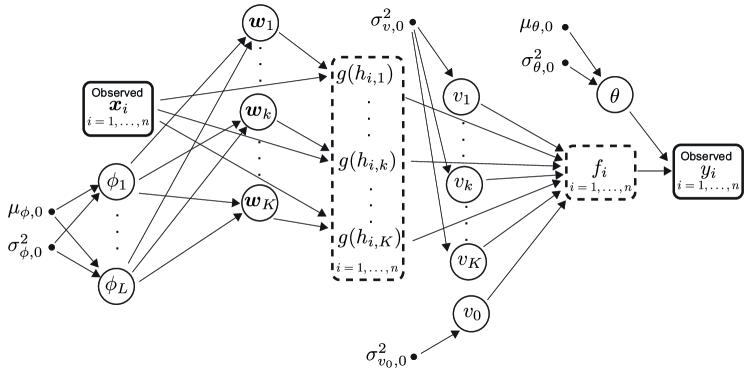
Figure 1: A directed graph representing the joint distribution of all the model parameters written in equation (7) resulting from the observation model and prior definitions summarized in Section 2. Observed variables indexed with $i=1,...,n$ are denoted with boxes, unobserved random variables are denoted with circles, and fixed prior parameters are denoted with dots. For each input $\mathbf{x}_{i}$, $i=1,...,n$, two intermediate random variables are visualized: The linear hidden unit activations defined as $h_{i,k}=\mathbf{w}_{k}^{\text{T}}\mathbf{x}_{i}$ and the latent function value given by $f_{i}=\sum_{k=1}^{K}v_{k}g(h_{i,k})+v_{0}$.

In this section, we describe how approximate Bayesian inference on the unknown model parameters $\mathbf{w}$, $\mathbf{v}$, $\theta$, and $\bm{\phi}=[\phi_{1},...,\phi_{L}]^{\text{T}}$ can be done efficiently using expectation propagation. First, the structure of the approximation and the expressions of the approximate site terms are presented in Section 3.1. A general description of the EP algorithm for determining the parameters of the site approximations is given in Section 3.2 and approximations for the non-Gaussian hierarchial weight priors are described in Section 3.2.1. The various computational blocks required in the EP algorithm are discussed first in Section 3.3 and detailed descriptions of the methods are given in Appendices A–E. Finally, an algorithm description with references to the different building blocks is given in 3.3.1.

3.1 The Structure of the Approximation

Given a set of $n$ observations $\mathcal{D}=\{\mathbf{X},\mathbf{y}\}$, where $\mathbf{y}=[y_{1},...,y_{n}]^{\text{T}}$, $\mathbf{X}=[\mathbf{x}_{1},...,\mathbf{x}_{n}]^{\text{T}}$, the posterior distribution of all the unknowns is given by

$$p(\mathbf{z},\theta,\bm{\phi}|\mathcal{D})= Z^{-1}\prod_{i=1}^{n}p(y_{i}|f_{i},\theta)\prod_{j=1}^{Kd}p(w_{j}|\phi_{l_{j}})\prod_{k=0}^{K}p(v_{k}|\sigma_{\mathbf{v},0}^{2})\prod_{l=1}^{L}p(\phi_{l})p(\theta),$$ (7)

where $\sigma_{\mathbf{v},0}^{2}=\{\sigma_{v,0}^{2},\sigma_{v_{0},0}^{2}\}$ and $Z=p(\mathbf{y}|\mathbf{X},\sigma_{\mathbf{v},0}^{2})$ is the marginal likelihood of the observed data conditioned on all fixed hyperparameters (in this case $\sigma_{\mathbf{v},0}^{2}$). Figure 1 shows a directed graph representing the joint distribution (7) where we have also included intermediate random variables $h_{i,k}=\mathbf{w}_{k}^{\text{T}}\mathbf{x}_{i}$ and $f_{i}$ related to each data point to clarify the upcoming description of the approximate inference scheme. To form an analytically tractable approximation, all non-Gaussian terms are approximated with unnormalized Gaussian site functions, which is a suitable approximating family for random vectors defined in the real vector space.

We first consider different possibilities for approximating the likelihood terms $p(y_{i}|f_{i},\theta)$ which depend on the unknown noise parameter $\theta=\log\sigma^{2}$ and the unknown weight vectors $\mathbf{w}$ and $\mathbf{v}$ through the latent function value $f_{i}$ according to:

$$f_{i}=\mathbf{v}^{\text{T}}\mathbf{g}(\tilde{\mathbf{x}}_{i}^{\text{T}}\mathbf{w})=\mathbf{v}^{\text{T}}\mathbf{g}(\mathbf{h}_{i}),$$ (8)

where $\tilde{\mathbf{x}}_{i}=\mathbf{I}_{K}\otimes\mathbf{x}_{i}$ is a $Kd\times K$ auxiliary matrix formed as Kronecker product. It can be used to write all the linear input layer activations $\mathbf{h}_{i}$ of observation $\mathbf{x}_{i}$ as $\mathbf{h}_{i}=\mathbf{h}(\mathbf{x}_{i})=\tilde{\mathbf{x}}_{i}^{\text{T}}\mathbf{w}$. The vector valued function $\mathbf{g}(\mathbf{h}_{i})$ applies the nonlinear transformation (2) on each component of $\mathbf{h}_{i}$ according to $\mathbf{g}(\mathbf{h}_{i})=[g(\mathbf{h}_{i,1}),g(\mathbf{h}_{i,2}),...,g(\mathbf{h}_{i,K}),1]^{\text{T}}$ (the last element corresponds to the output bias $v_{0}$). If we approximate the posterior distribution of all the weights $\mathbf{z}=[\mathbf{w}^{\text{T}},\mathbf{v}^{\text{T}}]^{\text{T}}$ with a multivariate Gaussian approximation that is independent of all the other unknowns including $\theta$, the resulting EP algorithm requires fast evaluation of the means and covariances of tilted distributions of the form

$$\hat{p}_{i}(\mathbf{z})\propto p(y_{i}|\mathbf{v}^{T}\mathbf{g}(\mathbf{h}_{i}),\theta)\mathcal{N}(\mathbf{z}|\bm{\mu}_{\mathbf{z}},\bm{\Sigma}_{\mathbf{z}}),$$ (9)

where $\bm{\mu}_{\mathbf{z}}$ is a known mean vector, and $\bm{\Sigma}_{\mathbf{z}}$ a known covariance matrix, and $\theta$ is assumed fixed. Because the non-Gaussian likelihood term depends on $\mathbf{z}$ only through linear transformation $\mathbf{h}_{i}$, it can be shown (by differentiating (9) twice with respect to $\bm{\mu}_{\mathbf{z}}$) that the normalization term, mean and covariance of $\hat{p}_{i}(\mathbf{z})$ can be exactly determined by using the corresponding moments of the transformed lower dimensional random vector $\mathbf{u}_{i}=\mathbf{B}_{i}^{\text{T}}\mathbf{z}=[\mathbf{w}^{\text{T}}\tilde{\mathbf{x}}_{i},\mathbf{v}^{\text{T}}]^{\text{T}}$, where the transformation matrix $\mathbf{B}_{i}$ can be written as

$$\mathbf{B}_{i}=\begin{bmatrix}\tilde{\mathbf{x}}_{i}&\mathbf{0}\\ \mathbf{0}&\mathbf{I}_{K+1}\\ \end{bmatrix}.$$ (10)

This results in significant computational savings because the size of $\mathbf{B}_{i}$ is $d_{z}\times d_{u}$, where we have denoted the dimensions of $\mathbf{u}_{i}$ and $\mathbf{z}$ with $d_{u}=2K+1$ and $d_{z}=Kd+K+1$ respectively. It follows that the EP algorithm can be implemented by propagating the moments of $\mathbf{u}_{i}$ using, for example, the general algorithm described by Cseke and Heskes (2011, appendix C). The same principle has been utilized to form computationally efficient algorithms also for linear binary classification (Minka, 2001b; Qi et al., 2004).

Independent Gaussian posterior approximations for both $\mathbf{z}$ and $\theta$ can be obtained by approximating the likelihood terms by a product of two unnormalized Gaussian site functions:

$$p(y_{i}|f_{i},\theta)\approx\tilde{Z}_{y,i}\tilde{t}_{\mathbf{z},i}(\mathbf{z})\tilde{t}_{\theta,i}(\theta),$$

where $\tilde{Z}_{y,i}$ is a scalar scaling parameter. Because of the previously described property, the first likelihood site approximation depends on $\mathbf{z}$ only through transformation $\mathbf{B}_{i}^{\text{T}}\mathbf{z}$ (Cseke and Heskes, 2011):

$$\tilde{t}_{\mathbf{z},i}(\mathbf{z})=\exp\left(-\frac{1}{2}\mathbf{z}^{\text{T}}\mathbf{B}_{i}\tilde{\mathbf{T}}_{i}\mathbf{B}_{i}^{\text{T}}\mathbf{z}+\mathbf{z}^{\text{T}}\mathbf{B}_{i}\tilde{\mathbf{b}}_{i}\right),$$ (11)

where $\tilde{\mathbf{b}}_{i}$ is a $d_{u}\times 1$ vector of location parameters, and $\tilde{\mathbf{T}}_{i}$ a $d_{u}\times d_{u}$ site precision matrix. The second likelihood site term dependent on the scalar $\theta=\log\sigma^{2}$ is chosen to be an unnormalized Gaussian

$$\tilde{t}_{\theta,i}(\theta)=\exp\left(-\frac{1}{2}\tilde{\sigma}_{\theta,i}^{-2}\theta^{2}+\tilde{\mu}_{\theta,i}\tilde{\sigma}_{\theta,i}^{-2}\theta\right)\propto\mathcal{N}(\theta|\tilde{\mu}_{\theta,i},\tilde{\sigma}_{\theta,i}^{2}),$$ (12)

where the site parameters $\tilde{\mu}_{\theta,i}$ and $\tilde{\sigma}_{\theta,i}^{2}$ control the location and the scale of site function, respectively. Combined with the known Gaussian prior term on $\theta$ this results in a Gaussian posterior approximation for $\theta$ that corresponds to a log-normal approximation for $\sigma^{2}$.

The prior terms of the output weights $v_{k}$, for $k=1,...,K$, are approximated with

$$p(v_{k}|\sigma_{v,0}^{2})\approx\tilde{Z}_{v,k}\tilde{t}_{v,k}(v_{k})\propto\mathcal{N}(v_{k}|\tilde{\mu}_{v,k},\tilde{\sigma}_{v,k}^{2}),$$ (13)

where $\tilde{Z}_{v,k}$ is a scalar scaling parameter, $\tilde{t}_{v,k}(v_{k})$ has a similar exponential form as (12), and the site parameters $\tilde{\mu}_{v,k}$ and $\tilde{\sigma}_{v,k}^{2}$ control the location and scale of the site, respectively. If the prior scales $\phi_{l}$ are assumed unknown, the prior terms of the input weights $\{w_{j}|j=1,...,Kd\}$, are approximated with

$$p(w_{j}|\phi_{l_{j}})\approx\tilde{Z}_{w,j}\tilde{t}_{w,j}(w_{j})\tilde{t}_{\phi,j}(\phi_{l_{j}})\propto\mathcal{N}(w_{j}|\tilde{\mu}_{w,j},\tilde{\sigma}_{w,j}^{2})\mathcal{N}(\phi_{l_{j}}|\tilde{\mu}_{\phi,j},\tilde{\sigma}_{\phi,j}^{2}),$$ (14)

where a factorized site approximation with location parameters $\tilde{\mu}_{w,j}$ and $\tilde{\mu}_{\phi,j}$, and scale parameters $\tilde{\sigma}_{w,j}^{2}$ and $\tilde{\sigma}_{\phi,j}^{2}$, is assumed for weight $w_{j}$ and the associated scale parameter $\phi_{l_{j}}$, respectively. A similar exponential form to equation (12) is assumed for both $\tilde{t}_{w,j}(w_{j})$ and $\tilde{t}_{\phi,j}(\phi_{l_{j}})$. This factorizing site approximation results in independent posterior approximations for $\mathbf{w}$ and each component of $\bm{\phi}$ as will be described shortly.

The actual numerical values of the normalization parameters $\tilde{Z}_{y,i}$, $\tilde{Z}_{v,k}$, and $\tilde{Z}_{w,j}$ are not required during the iterations of the EP algorithm but their effect must be taken into account if one wishes to form an EP approximation for the marginal likelihood $Z=p(\mathbf{y}|\mathbf{X})$ (see Appendix G). This estimate could be utilized to compare models or to alternatively determine type-II MAP estimates for hyperparameters $\theta$, $\{\phi_{l}\}_{l=1}^{L}$, and $\sigma_{v,0}^{2}$ in case they are not inferred within the EP framework.

3.1.1 Fully-coupled approximation for the network weights

Multiplying the site approximations together according to (7) and normalizing the resulting expression gives the following Gaussian posterior approximation:

$$p(\mathbf{z},\theta,\bm{\phi}|\mathcal{D},\sigma_{\mathbf{v},0}^{2})\approx q(\mathbf{z})q(\theta)\prod_{l=1}^{L}q(\phi_{l}),$$ (15)

where $q(\mathbf{z})=\mathcal{N}(\mathbf{z}|\bm{\mu},\bm{\Sigma})$, $q(\theta)=\mathcal{N}(\theta|\mu_{\theta}^{2},\sigma_{\theta}^{2})$, and $q(\phi_{l})=\mathcal{N}(\phi_{l}|\mu_{\phi_{l}}^{2},\sigma_{\phi_{l}}^{2})$ are the approximate posterior distributions of the weights $\mathbf{z}$, the noise parameter $\theta=\log\sigma^{2}$, and the input weight scale parameter $\phi_{l}$, respectively. The mean vector and covariance matrix of $q(\mathbf{z})$, are given by

$$\bm{\Sigma}=\left(\sum_{i}^{n}\mathbf{B}_{i}\tilde{\mathbf{T}}_{i}\mathbf{B}_{i}^{\text{T}}+\bm{\Sigma}_{0}^{-1}\right)^{-1}\quad\textrm{and}\quad\bm{\mu}=\bm{\Sigma}\left(\sum_{i}^{n}\mathbf{B}_{i}\tilde{\mathbf{b}}_{i}+\bm{\Sigma}_{0}^{-1}\bm{\mu}_{0}\right),$$ (16)

where the parameters of the prior term approximations (13) and (14) are collected together in $\bm{\Sigma}_{0}=\text{diag}([\tilde{\sigma}_{w,1}^{2},...,\tilde{\sigma}_{w,Kd}^{2},\tilde{\sigma}_{v,1}^{2},...,\tilde{\sigma}_{v,K}^{2}])$ and $\bm{\mu}_{0}=[\tilde{\mu}_{w,1},...,\tilde{\mu}_{w,Kd},\tilde{\mu}_{v,1},...,\tilde{\mu}_{v,K}]^{\text{T}}$. The parameters of $q(\theta)$ are given by

$$\sigma_{\theta}^{2}=\left(\sum_{i}^{n}\tilde{\sigma}_{\theta,i}^{-2}+\sigma_{\theta,0}^{-2}\right)^{-1}\quad\textrm{and}\quad\mu_{\theta}=\sigma_{\theta,0}^{2}\left(\sum_{i}^{n}\tilde{\sigma}_{\theta,i}^{-2}\tilde{\mu}_{\theta,i}+\sigma_{\theta,0}^{-2}\mu_{\theta,0}\right).$$ (17)

The approximate mean and variance of $q(\phi_{l})$ can be computed analogously to (17). The key property of the approximation (15) is that if we can incorporate the information provided by the data point $y_{i}$ in the parameters $\tilde{\mathbf{T}}_{i}$ and $\tilde{\mathbf{b}}_{i}$, for all $i=1,\ldots,n$, the approximate inference on the non-Gaussian priors $p(v_{k})$ and $p(w_{kj})$ is straightforward by adopting the methods described by (Seeger, 2008). In the following sections we will show how this can be done by approximating the joint distribution of $f_{i}$, $\mathbf{h}_{i}$ and $\mathbf{v}$, given $\mathbf{y}_{-i}=[y_{1},...,y_{i-1},y_{i+1},...,y_{n}]$, with a multivariate Gaussian and using it to estimate the parameters $\tilde{\mathbf{T}}_{i}$ and $\tilde{\mathbf{b}}_{i}$ one data point at a time within the EP framework.

3.1.2 Factorizing approximation for the network weights

A drawback with the approximation (16) is that the evaluation of the covariance matrix $\bm{\Sigma}$ scales as $\mathcal{O}(\min(Kd+K+1,n)^{3})$ which may not be feasible when the number of inputs $d$ is large. Another difficulty arises in determining the mean and covariance of $\mathbf{u}_{i}=\mathbf{B}_{i}\mathbf{z}=[\mathbf{h}_{i}^{\text{T}},\mathbf{v}^{\text{T}}]^{\text{T}}$ when $\mathbf{z}$ is distributed according to (9) because during the EP iterations $\bm{\Sigma}_{\mathbf{z}}$ has similar correlation structure with $\bm{\Sigma}$. If the observation model is Gaussian and $\theta$ is fixed, this requires at least $K$-dimensional numerical quadratures (or other alternative approximations) that may quickly become infeasible as $K$ increases. By adopting suitable independence assumptions between $\mathbf{v}$ and the input weights $\mathbf{w}_{k}$ associated with the different hidden units, the mean and covariance of $\mathbf{u}_{i}$ can be approximated using only 1-dimensional numerical quadratures as will be described in Section 3.3.

The structure of the correlations in the approximation $\eqref{eq_qep_z}$ can be studied by dividing $\tilde{\mathbf{T}}_{i}$ into four blocks as follows:

$$\tilde{\mathbf{T}}_{i}=\left[\begin{array}[]{cc}\tilde{\mathbf{T}}_{\mathbf{h}_{i}\mathbf{h}_{i}}&\tilde{\mathbf{T}}_{\mathbf{h}_{i}\mathbf{v}}\\ \tilde{\mathbf{T}}_{\mathbf{h}_{i}\mathbf{w}}&\tilde{\mathbf{T}}_{i,\mathbf{v}\mathbf{v}}\\ \end{array}\right],$$ (18)

where $\tilde{\mathbf{T}}_{\mathbf{h}_{i}\mathbf{h}_{i}}$ is a $K\times K$ matrix, $\tilde{\mathbf{T}}_{\mathbf{h}_{i}\mathbf{v}}$ a $K\times K+1$ matrix, and $\tilde{\mathbf{T}}_{i,\mathbf{v}\mathbf{v}}$ a $K+1\times K+1$ matrix. The element $[\tilde{\mathbf{T}}_{\mathbf{h}_{i}\mathbf{h}_{i}}]_{k,k^{\prime}}$ contributes to the approximate posterior covariance between $\mathbf{w}_{k}$ and $\mathbf{w}_{k^{\prime}}$, and the sub-matrix $\tilde{\mathbf{T}}_{\mathbf{h}_{i}\mathbf{v}}$ contributes to the approximate covariance between $\mathbf{w}$ and $\mathbf{v}$. To form an alternative computationally more efficient approximation we propose a simpler structure for $\tilde{\mathbf{T}}_{i}$. First, we approximate $\tilde{\mathbf{T}}_{\mathbf{h}_{i}\mathbf{h}_{i}}$ with a diagonal matrix, that is, $\tilde{\mathbf{T}}_{\mathbf{h}_{i}\mathbf{h}_{i}}=\textrm{diag}(\tilde{\bm{\tau}}_{i})$, where only the $k$:th component of the vector $\tilde{\bm{\tau}}_{i}$ contributes to the posterior covariance of $\mathbf{w}_{k}$. Secondly, we set $\tilde{\mathbf{T}}_{\mathbf{h}_{i}\mathbf{v}}=\bm{0}$ and approximate $\tilde{\mathbf{T}}_{i,\mathbf{v}\mathbf{v}}$ with an outer-product of the form $\tilde{\mathbf{T}}_{i,\mathbf{v}\mathbf{v}}=\tilde{\bm{\alpha}}_{i}\tilde{\bm{\alpha}}_{i}^{\text{T}}$. With this precision structure the site approximation (11) can be factorized into terms depending only on the output weights $\mathbf{v}$ or the input weights $\mathbf{w}_{k}$ associated with the different hidden units $k=1,...,K$:

$$\tilde{t}_{\mathbf{z},i}(\mathbf{z}) =\exp\left(-\frac{1}{2}(\tilde{\bm{\alpha}}_{i}^{\text{T}}\mathbf{v})^{2}+\mathbf{v}^{\text{T}}\tilde{\bm{\beta}}_{i}\right)\prod_{k=1}^{K}\exp\left(-\frac{1}{2}\tilde{\tau}_{i,k}(\mathbf{x}_{i}^{\text{T}}\mathbf{w}_{k})^{2}+\tilde{\nu}_{i,k}\mathbf{w}_{k}^{\text{T}}\mathbf{x}_{i}\right)$$ (19)

$$=\tilde{t}_{\mathbf{v},i}(\mathbf{v})\prod_{k=1}^{K}\tilde{t}_{\mathbf{w}_{k},i}(\mathbf{w}_{k}),$$

where the site location parameters $\tilde{\nu}_{i,k}$ now correspond to the first $K$ elements of $\tilde{\mathbf{b}}_{i}$ in equation (11), that is, $\tilde{\bm{\nu}}_{i}=[\tilde{\nu}_{i,1},...\tilde{\nu}_{i,K}]^{\text{T}}=[\tilde{\mathbf{b}}_{i,1},...,\tilde{\mathbf{b}}_{i,K}]^{\text{T}}$. Analogously, the site location vector $\tilde{\bm{\beta}}_{i}$ corresponds to the last $K+1$ entries of $\tilde{\mathbf{b}}_{i}$, that is, $\tilde{\bm{\beta}}_{i}=[\tilde{\mathbf{b}}_{i,K+1},...,\tilde{\mathbf{b}}_{i,2K+1}]^{\text{T}}$.

The factored site approximation (19) results in independent posterior approximations for the output weights $\mathbf{v}$ and the input weights $\mathbf{w}_{k}$ associated with different hidden units:

$$q(\mathbf{z})=q(\mathbf{v})\prod_{k=1}^{K}q(\mathbf{w}_{k}),$$ (20)

where $q(\mathbf{v})=\mathcal{N}(\bm{\mu}_{v},\bm{\Sigma}_{v})$ and $q(\mathbf{w}_{k})=\mathcal{N}(\bm{\mu}_{\mathbf{w}_{k}},\bm{\Sigma}_{\mathbf{w}_{k}})$. The approximate mean and covariance of $\mathbf{w}_{k}$ is given by

$$\bm{\Sigma}_{\mathbf{w}_{k}}=\left(\mathbf{X}^{\text{T}}\tilde{\mathbf{T}}_{\mathbf{w}_{k}}\mathbf{X}+\bm{\Sigma}_{\mathbf{w}_{k},0}^{-1}\right)^{-1}\quad\textrm{and}\quad\bm{\mu}_{\mathbf{w}_{k}}=\bm{\Sigma}_{\mathbf{w}_{k}}\left(\mathbf{X}^{\text{T}}\tilde{\bm{\nu}}_{\mathbf{w}_{k}}+\bm{\Sigma}_{\mathbf{w}_{k},0}^{-1}\bm{\mu}_{\mathbf{w}_{k},0}\right),$$ (21)

where the diagonal matrix $\tilde{\mathbf{T}}_{\mathbf{w}_{k}}=\textrm{diag}(\tilde{\bm{\tau}}_{\mathbf{w}_{k}})$ and the vector $\tilde{\bm{\nu}}_{\mathbf{w}_{k}}$ collect all the site parameters related to hidden unit $k$: $\tilde{\bm{\tau}}_{\mathbf{w}_{k}}=[\tilde{\tau}_{1,k},...,\tilde{\tau}_{n,k}]^{\text{T}}$ and $\tilde{\bm{\nu}}_{\mathbf{w}_{k}}=[\tilde{\nu}_{1,k},...,\tilde{\nu}_{n,k}]^{\text{T}}$. The diagonal matrix $\bm{\Sigma}_{\mathbf{w}_{k},0}$ and the vector $\bm{\mu}_{\mathbf{w}_{k},0}$ contain the prior site scales $\tilde{\sigma}_{w,j}^{2}$ and the location variables $\tilde{\mu}_{w,j}$ related to the hidden unit $k$. The approximate mean and covariance of the output weights $\mathbf{v}$ are given by

$$\bm{\Sigma}_{\mathbf{v}}=\left(\sum_{i=1}^{n}\tilde{\bm{\alpha}}_{i}\tilde{\bm{\alpha}}_{i}^{\text{T}}+\bm{\Sigma}_{\mathbf{v},0}^{-1}\right)^{-1}\quad\textrm{and}\quad\bm{\mu}_{\mathbf{v}}=\bm{\Sigma}_{\mathbf{v}}\left(\sum_{i=1}^{n}\tilde{\bm{\beta}}_{i}+\bm{\Sigma}_{\mathbf{v}}^{-1}\bm{\mu}_{\mathbf{v},0}\right),$$ (22)

where the diagonal matrix $\bm{\Sigma}_{\mathbf{v},0}$ and the vector $\bm{\mu}_{\mathbf{v},0}$ contain the prior site scales $\tilde{\sigma}_{v,j}^{2}$ and the location variables $\tilde{\mu}_{v,j}$.

For each hidden unit $k$, approximations (20) and (21) can be interpreted as independent linear models with Gaussian likelihood terms $\mathcal{N}(\tilde{y}_{i,k}|\mathbf{x}_{i}^{\text{T}}\mathbf{w}_{k},\tilde{\tau}_{i,k}^{-1})$, where the pseudo-observations are given by $\tilde{y}_{i,k}=\tilde{\tau}_{i,k}^{-1}\tilde{\nu}_{i,k}$. The approximation for the output weights (22) has no explicit dependence on the input vectors $\mathbf{x}_{i}$ but later we will show that the independence assumption results in a similar dependence on expected values of $\mathbf{g}_{i}$ taken with respect to approximate leave-one-out (LOO) distributions of $\mathbf{w}$ and $\mathbf{v}$.

3.2 Expectation Propagation

The parameters of the approximate posterior distribution (15) are determined using the EP algorithm (Minka, 2001a). The EP algorithm updates the site parameters and the posterior approximation $q(\mathbf{z},\theta,\bm{\phi})$ sequentially. In the following, we briefly describe the procedure for updating the likelihood sites $\tilde{t}_{\mathbf{z},i}$ and $\tilde{t}_{\theta,i}$ and assume that the prior sites (13) and (14) are kept fixed. Because the likelihood terms $p(y_{i}|f_{i},\theta)$ do not depend on $\bm{\phi}$ and posterior approximation is factorized, that is $q(\mathbf{z},\theta,\bm{\phi})=q(\mathbf{z})q(\theta)q(\bm{\phi})$, we need to consider only the approximations for $\mathbf{z}$ and $\theta$. Furthermore, independent approximations for $\mathbf{w}_{k}$ and $\mathbf{v}$ are obtained by using (19) and (20) in place $\tilde{t}_{\mathbf{z},i}$ and $q(\mathbf{z})$, respectively.

At each iteration, first a proportion $\eta$ of the $i$:th site term is removed from the posterior approximation to obtain a cavity distribution:

$$q_{-i}(\mathbf{z},\theta)=q_{-i}(\mathbf{z})q_{-i}(\theta)\propto q(\mathbf{z})q(\theta)\tilde{t}_{\mathbf{z},i}(\mathbf{z})^{-\eta}\tilde{t}_{\theta,i}(\theta)^{-\eta},$$ (23)

where $\eta\in(0,1]$ is a fraction parameter that can be adjusted to implement fractional (or power) EP updates (Minka, 2004, 2005). When $\eta=1$, the cavity distribution (23) can be thought of as a LOO posterior approximation where the contribution of the $i$:th likelihood term $p(y_{i}|f_{i},\theta)$ is removed from $q(\mathbf{z},\theta)$. Then, the $i$:th site is replaced with the exact likelihood term to form a tilted distribution

$$\hat{p}_{i}(\mathbf{z},\theta)=\hat{Z}_{i}^{-1}q_{-i}(\mathbf{z},\theta)p(y_{i}|\mathbf{z},\theta,\mathbf{x})^{\eta},$$ (24)

where $\hat{Z}_{i}$ is a normalization constant, which in this case can also be thought of as an approximation for the LOO predictive density of the excluded data point $y_{i}$. The tilted distribution can be regarded as a more refined non-Gaussian approximation to the true posterior distribution. Next, the algorithm attempts to match the approximate posterior distribution $q(\mathbf{z},\theta)$ with $\hat{p}_{i}(\mathbf{z},\theta)$ by finding first a Gaussian $\hat{q}_{i}(\mathbf{z},\theta)$ that satisfies

$$\hat{q}_{i}(\mathbf{z},\theta)=\operatorname{arg\,min}_{q_{i}}\operatorname{KL}\left(\hat{p}_{i}(\mathbf{z},\theta)||q_{i}(\mathbf{z},\theta)\right),$$

where KL denotes the Kullback-Leibler divergence. When $q(\mathbf{z},\theta)$ is chosen to be a Gaussian distribution this is equivalent to determining the mean vector and the covariance matrix of $\hat{p}_{i}$ and matching them with the mean and covariance of $\hat{q}_{i}$. Then, the parameters of the $i$:th site terms are updated so that the moments of $q(\mathbf{z},\theta)$ match with $\hat{q}(\mathbf{z},\theta)$:

$$\hat{q}_{i}(\mathbf{z},\theta)\equiv q(\mathbf{z},\theta)\propto q_{-i}(\mathbf{z})q_{-i}(\theta)\tilde{t}_{\mathbf{z},i}(\mathbf{z})^{\eta}\tilde{t}_{\theta,i}(\theta)^{\eta}.$$ (25)

Finally, the posterior approximation $q(\mathbf{z},\theta)$ is updated according to the changes in the site parameters. These steps are repeated for all sites in some suitable order until convergence.

From now on, we refer to the previously described EP update scheme as sequential EP. If the update of the posterior approximation $q(\mathbf{z},\theta)$ in the last step is done only after new parameter values have been determined for all sites (in this case the $n$ likelihood term approximations), we refer to parallel EP (see, e.g., van Gerven et al., 2009). Because in our case the approximating family is Gaussian and each likelihood term depends on a linear transformation of $\mathbf{z}$, one sequential EP iteration requires (for each of the $n$ sites) either one rank-$(2K+1)$ covariance matrix update with the fully-correlated approximation (16), or $K+1$ rank-one covariance matrix updates with the factorized approximation (21, 22). In parallel EP these updates are replaced with a single re-computation of the posterior representation after each sweep over all the $n$ sites. In practice, one parallel iteration step over all the sites can be much faster compared to a sequential EP iteration, especially if $d$ or $K$ are large, but parallel EP may require larger number of iterations for overall convergence.

Setting the fraction parameter to $\eta=1$ corresponds to regular EP updates whereas choosing a smaller value produces a slightly different approximation that puts less emphasis on preserving all the nonzero probability mass of the tilted distributions (Minka, 2005). Consequently, setting $\eta<1$ tries to represent possible multimodalities in (24) but ignores modes far away from the main probability mass, which results in tendency to underestimate variances. However, in practice decreasing $\eta$ can improve the overall numerical stability of the algorithm and alleviate convergence problems resulting from possible multimodalities in case the unimodal approximation is not a good fit for the true posterior distribution (Minka, 2005; Seeger, 2008; Jylänki et al., 2011).

There is no theoretical convergence guarantee for the standard EP algorithm but damping the site parameter updates can help to achieve convergence in harder problems (Minka and Lafferty, 2002; Heskes and Zoeter, 2002). In damping, the site parameters are updated to a convex combination of the old values and the new values resulting from (25) defined by a damping factor $\delta\in(0,1]$. For example, the precision parameter of the likelihood site term $\tilde{t}_{\mathbf{w}_{k},i}$ is updated as $\tilde{\tau}_{i,k}=(1-\delta)\tilde{\tau}_{i,k}^{\text{old}}+\delta\tilde{\tau}_{i,k}^{\text{new}}$ and a similar update using the same $\delta$-value is done on the corresponding location parameter $\tilde{\nu}_{i,k}$. The convergence problems are usually seen as oscillations over iterations in the site parameter values and they may occur, for example, if there are inaccuracies in the tilted moment evaluations, or if the approximate distribution is not a suitable proxy for the true posterior, for example, due to multimodalities.

3.2.1 EP approximation for the weight prior terms

Assuming fixed site parameters for the likelihood approximation (19), or (11) in the case of full couplings, the EP algorithm for determining the prior term approximations (13) and (14) can be implemented in the same way as with sparse linear models (Seeger, 2008).

To derive EP updates for the non-Gaussian prior sites of the output weights $\mathbf{v}$ assuming the factorized approximation, we need to consider only the prior site approximations (13) and the approximate posterior $q(\mathbf{v})=\mathcal{N}(\mathbf{v}|\bm{\mu}_{\mathbf{v}},\bm{\Sigma}_{\mathbf{v}})$ defined in equation (22). All approximate posterior information from the observations $\mathcal{D}=\{\mathbf{y},\mathbf{X}\}$ and the priors on the input weights $\mathbf{w}$ are conveyed in the parameters $\{\tilde{\bm{\alpha}}_{i},\tilde{\bm{\beta}}_{i}\}_{i=1}^{n}$ determined during the EP iterations for the likelihood sites. The EP implementation of Seeger (2008) can be readily applied by using $\sum_{i}^{n}\tilde{\bm{\alpha}}_{i}\tilde{\alpha}_{i}^{\text{T}}$ and $\sum_{i}^{n}\tilde{\bm{\beta}}_{i}$ as a Gaussian pseudo likelihood as discussed in Appendix E. Because the prior terms $p(v_{k}|\sigma_{v,0}^{2})$ depend only on one random variable $v_{k}$, deriving the parameters of the cavity distributions $q_{-k}(v_{k})\propto q(v_{k})\tilde{t}_{v,k}(v_{k}|\tilde{\mu}_{v,k},\tilde{\sigma}_{v,k}^{2})^{-\eta}$ and updates for the site parameters $\tilde{\mu}_{v,k}$ and $\tilde{\sigma}_{v,k}^{2}$ require only manipulating univariate Gaussians. The moments of the tilted distribution $\hat{p}_{k}(v_{k})\propto q_{-k}(v_{k})p(v_{k}|\sigma_{v,0}^{2})^{\eta}$ can be computed either analytically or using a one-dimensional numerical quadrature depending on the functional form of the exact prior term $p(v_{k}|\sigma_{v,0}^{2})$.

To derive EP updates for the non-Gaussian hierarchical prior sites of the input weights $\mathbf{w}$ assuming the factorized approximation (20), we can consider the approximate posterior distributions $q(\mathbf{w}_{k})=\mathcal{N}(\mathbf{w}_{k}|\bm{\mu}_{\mathbf{w}_{k}},\bm{\Sigma}_{\mathbf{w}_{k}})$ from equation (21) separately with the corresponding prior site approximations (14) related to the $d$ components of $\mathbf{w}_{k}$. All approximate posterior information from the observations $\mathbf{y}$ is conveyed by the site parameters $\{\tilde{\bm{\tau}}_{\mathbf{w}_{k}},\tilde{\bm{\nu}}_{\mathbf{w}_{k}}\}$ that together with the input features form a Gaussian pseudo likelihood with a precision matrix $\mathbf{X}^{\text{T}}\textrm{diag}(\tilde{\bm{\tau}}_{\mathbf{w}_{k}})\mathbf{X}$ and location term $\mathbf{X}^{\text{T}}\tilde{\bm{\nu}}_{\mathbf{w}_{k}}$ (compare with equation 21). It follows that the EP implementation of Seeger (2008) can be applied to update the approximations $q(\mathbf{w}_{k})$ but, in addition, we have to derive site updates also for the scale parameter approximations $q(\phi_{l_{j}})$. EP algorithms for sparse linear models that operate on exact site terms depending on a nonlinear combination of multiple random variables have been proposed by Hernández-Lobato et al. (2008) and van Gerven et al. (2009).

Because the $j$:th exact prior term (3) depends on both the weight $w_{j}$ and the corresponding log-transformed scale parameter $\phi_{l_{j}}$, the $j$:th cavity distribution is formed by removing a fraction $\eta$ of both site approximations $\tilde{t}_{w,j}(w_{j})$ and $\tilde{t}_{\phi,j}(\phi_{l_{j}})$:

$$q_{-j}(w_{j},\phi_{l_{j}})=q_{-j}(w_{j})q_{-j}(\phi_{l_{j}})\propto q(w_{j})q(\phi_{l_{j}})\tilde{t}_{w,j}(w_{j})^{-\eta}\tilde{t}_{\phi,j}(\phi_{l_{j}})^{-\eta},$$ (26)

where $q(w_{j})$ is the $j$:th marginal approximation extracted from the corresponding approximation $q(\mathbf{w}_{k})$, and the approximate posterior for $\phi_{l_{j}}$ is formed by combining the prior (4) with all the site terms $\tilde{t}_{\phi,i}(\phi_{l_{i}})$ that depend on $\phi_{l_{i}}$:

$$q(\phi_{l_{j}})\propto p(\phi_{l_{j}})\prod_{i=1,l_{i}=l_{j}}^{Kd}\tilde{t}_{\phi,i}(\phi_{l_{i}}).$$

The $j$:th tilted distribution is formed by replacing the removed site terms with a fraction $\eta$ of the exact prior term $p(w_{j}|\phi_{l_{j}})$:

$$\hat{p}_{j}(w_{j},\phi_{l_{j}})=\hat{Z}_{w_{j}}^{-1}q_{-j}(w_{j})q_{-j}(\phi_{l_{j}})p(w_{j}|\phi_{l_{j}})^{\eta}\equiv\hat{q}(w_{j},\phi_{l_{j}}),$$ (27)

where $\hat{q}(w_{j},\phi_{l_{j}})$ is a Gaussian approximation formed by determining the mean and covariance of $\hat{p}_{j}(w_{j},\phi_{l_{j}})$. The site parameters are updated so that the resulting posterior approximation is consistent with the marginal means and variances of $\hat{q}(w_{j},\phi_{l_{j}})$:

$$\hat{q}_{j}(w_{j})\hat{q}_{j}(\phi_{l_{j}})=q_{-j}(w_{j})q_{-j}(\phi_{l_{j}})\tilde{t}_{w,j}(w_{j})^{\eta}\tilde{t}_{\phi,j}(\phi_{l_{j}})^{\eta}.$$ (28)

Because of the factorized approximation, the cavity computations (26) and the site updates (27) require only scalar operations similar to the evaluations of $q_{-i}(h_{i,k})$ and to the updates of $\{\tilde{\bm{\tau}}_{i},\tilde{\bm{\nu}}_{i}\}$ in equations (A) and (46) respectively (see Appendix A and E).

Determining the moments of (27) can be done efficiently using one-dimensional quadratures if the means and variances of $w_{j}$ with respect to the conditional distribution $\hat{p}_{j}(w_{j}|\phi_{l_{j}})$ can be determined analytically. This can be readily done when $p(w_{j}|\phi_{l_{j}})$ is a Laplace distribution or a finite mixture of Gaussians. Note also that if we wish to implement an ARD prior we can choose simply $p(w_{j}|\phi_{l_{j}})=\mathcal{N}(w_{j}|0,\phi_{l_{j}})$, where $\phi_{l_{j}}$ is a common scale parameter for all weights related to the same input feature, that is, weights $\{w_{j},w_{j+d},...,w_{j+(K-1)d}\}$, for each $j\in\{1,2,...,d\}$, share the same scale $\phi_{j}$. The marginal tilted distribution for $\phi_{l_{j}}$ is given by

$$\hat{p}(\phi_{l_{j}}) =\hat{Z}_{w_{j}}^{-1}\int q_{-j}(w_{j})q_{-j}(\phi_{l_{j}})p(w_{j}|\phi_{l_{j}})^{\eta}dw_{j}=\hat{Z}_{w_{j}}^{-1}Z(\phi_{l_{j}},\eta)q_{-j}(\phi_{l_{j}})$$

$$\approx\mathcal{N}(\phi_{l_{j}}|\hat{\mu}_{\phi,l_{j}},\hat{\sigma}_{\phi,l_{j}}^{2}),$$ (29)

where it is assumed that $Z(\phi_{l_{j}},\eta)=\int q_{-j}(w_{j})p(w_{j}|\phi_{l_{j}})^{\eta}dw_{j}$ can be calculated analytically. The normalization term $\hat{Z}_{w_{j}}^{-1}$, the marginal mean $\hat{\mu}_{\phi,l_{j}}$, and the variance $\hat{\sigma}_{\phi,l_{j}}^{2}$ can be determined using numerical quadratures.

The marginal tilted mean and variance of $w_{j}$ can be determined by integrating numerically the conditional expectations of $w_{j}$ and $w_{j}^{2}$ over $\hat{p}_{j}(\phi_{l_{j}})$:

$$\operatorname{E}(w_{j}) =\hat{Z}_{w_{j}}^{-1}\int w_{j}\hat{p}_{j}(w_{j}|\phi_{l_{j}})Z(\phi_{l_{j}},\eta)q_{-j}(\phi_{l_{j}})dw_{j}d\phi_{l_{j}}=\int\operatorname{E}(w_{j}|\phi_{l_{j}},\eta)\hat{p}_{j}(\phi_{l_{j}})d\phi_{l_{j}}$$

$$\operatorname{Var}(w_{j}) =\int\operatorname{E}(w_{j}^{2}|\phi_{l_{j}},\eta)\hat{p}_{j}(\phi_{l_{j}})d\phi_{l_{j}}-\operatorname{E}(w_{j})^{2},$$ (30)

where $\hat{p}_{j}(w_{j}|\phi_{l_{j}})=Z(\phi_{l_{j}},\eta)^{-1}q_{-j}(w_{j})p(w_{j}|\phi_{l_{j}})^{\eta}$, and it is assumed that the conditional expectations $\operatorname{E}(w_{j}|\phi_{l_{j}},\eta)$ and $\operatorname{E}(w_{j}^{2}|\phi_{l_{j}},\eta)$ can be calculated analytically. For prior distributions $p(w_{j}|\phi_{l_{j}})$ belonging to the exponential family, the exponentiation with $\eta$ results in a distribution of the same family multiplied by a function of $\eta$ and $\phi_{l_{j}}$. Evaluating the marginal moments according to equations (3.2.1) and (3.2.1) requires a total of five one-dimensional quadrature integrations but in practice this can be done efficiently by utilizing the same function evaluations of $\hat{p}_{j}(\phi_{l_{j}})$ and taking into account the prior specific forms of $\operatorname{E}(w_{j}|\phi_{l_{j}},\eta)$ and $\operatorname{E}(w_{j}^{2}|\phi_{l_{j}},\eta)$.

3.3 Implementing the EP Algorithm

In this section, we describe the computational implementation of the EP algorithm resulting from the choice of the approximating family described in Section 3.1. Because the non-Gaussian likelihood term in the tilted distribution (24) depends on $\mathbf{z}=[\mathbf{w}^{\text{T}},\mathbf{v}^{\text{T}}]^{\text{T}}$ only through the linear transformation $\mathbf{u}_{i}=[\mathbf{h}_{i}^{\text{T}},\mathbf{v}^{\text{T}}]^{\text{T}}=\mathbf{B}_{i}^{\text{T}}\mathbf{z}$, the EP algorithm can be more efficiently implemented by iteratively determining and matching the moments of the lower-dimensional random vector $\mathbf{u}_{i}$ instead of $\mathbf{z}$ (Cseke and Heskes, 2011, appendix C). The computations can be further facilitated by using the factorized approximation (20): Because the hidden activations $h_{i,k}=\mathbf{x}_{i}^{\text{T}}\mathbf{w}_{k}$ related to different hidden units $k=1,...,K$ are independent of each other and $\mathbf{v}$, it is only required to propagate the marginal means and covariances of $h_{i,k}$ and $\mathbf{v}$ to determine the new site parameters. This results in computationally more efficient determination of the cavity distributions (23), the tilted distributions (24), and the new site parameter from (25). Details of the computations required for updating the likelihood site approximations are presented in Appendices A–E. The main properties of the procedure can be summarized as:

• Appendix A presents the formulas for computing the parameters of the cavity distributions (23). The factorized approximation (20) leads to efficient computations, because the cavity distribution can be factored as $q_{-i}(\mathbf{z})=q_{-i}(\,\mathbf{v})\prod_{k=1}^{K}q_{-i}(\mathbf{w}_{k})$. The parameters of $q_{-i}(h_{i,k})$ resulting from the transformation $h_{i,k}=\mathbf{x}_{i}^{\text{T}}\mathbf{w}_{k}$ can be computed using only scalar manipulations of the mean and covariance of $q(h_{i,k})=\mathcal{N}(\mathbf{x}_{i}^{\text{T}}\bm{\mu}_{\mathbf{w}_{k}},\mathbf{x}_{i}^{\text{T}}\bm{\Sigma}_{\mathbf{w}_{k}}\mathbf{x}_{i})$. Because of the outer-product structure of $\tilde{t}_{\mathbf{v},i}(\mathbf{v})$ in equation (19), also the parameters of $q_{-i}(\mathbf{v})$ can be computed using rank-one matrix updates.

• Appendix B describes how the marginal mean and covariance of $\mathbf{v}$ with respect to the tilted distribution (24) can be approximated efficiently using a similar approach as in the UKF filter (Wan and van der Merwe, 2000). Because of the factorized approximation (20) only one-dimensional quadratures are required to compute the means and variances of $g(h_{i,k})$ with respect to $q_{-i}(h_{i,k})$ and no multivariate quadrature or sigma-point approximations are needed.

• Appendix C presents a new way to approximate the marginal distribution of $\hat{p}_{i}(h_{i,k})$ resulting from (24). In preliminary simulations we found that a more simple approach based on the unscented transform and the approximate linear filtering paradigm did not capture well the information from the left-out observation $y_{i}$. This behavior was more problematic when there was a large discrepancy between the information provided by the likelihood term through the marginal tilted distribution $\hat{p}_{i}(y_{i}|h_{i,k})=\int p(y_{i}|f_{i},\theta)^{\eta}q_{-i}(\mathbf{v})q_{-i}(\mathbf{h}_{i,-k})d\mathbf{v}d\mathbf{h}_{i,-k}$ and the cavity distribution $q_{-i}(h_{i,k})$, where $\mathbf{h}_{i,-k}$ includes all components of $\mathbf{h}_{i}$ except $h_{i,k}$. The improved numerical approximation of $\hat{p}_{i}(h_{i,k})$ is obtained by approximating $q_{-i}(f_{i}|h_{i,k})$, that is, the distribution of the latent function value $f_{i}=\sum_{k=1}^{K}g(h_{i,k})+v_{0}$ resulting from $q_{-i}(\mathbf{h}_{i,-k},\mathbf{v}|h_{i,k})=q_{-i}(\mathbf{v})\prod_{k^{\prime}\neq k}q_{-i}(h_{i,-k})$, with a Gaussian distribution and carrying out the integration over $f_{i}$ analytically. According to the central limit theorem we expect this approximation to get more accurate as $K$ increases.

• Appendix D generalizes the tilted moment estimations of Appendices B and C for approximate integration over the posterior uncertainty of $\theta=\log\sigma^{2}$. Computationally convenient marginal mean and covariance estimates for $\mathbf{v}$, $\{h_{i,k}\}_{k=1}^{K}$, and $\theta$ can be obtained by assuming an independent posterior approximation for $\theta$ and making a similar Gaussian approximation for $q_{-i}(f_{i})$ as in Appendix C. Compared to the tilted moments approximations of $\mathbf{v}$ and $\mathbf{h}_{i}$ with fixed $\theta$, the approach requires five additional univariate quadratures for each likelihood term, which can be facilitated by utilizing the same function evaluations.

• Appendix E presents expressions for the new site parameters obtained by applying the results of Appendices A–D in the moment matching condition (25). Because of the factorization assumption in (20) and the UKF-style approximation in the tilted moment estimations (Appendix B), the parameters of the likelihood term approximations related to $\mathbf{v}$ can be written as $\tilde{\bm{\alpha}}_{i}=\mathbf{m}_{\mathbf{g}_{i}}\tilde{\sigma}_{\mathbf{v},i}^{-1}$ and $\tilde{\bm{\beta}}_{i}=\mathbf{m}_{\mathbf{g}_{i}}\tilde{\sigma}_{\mathbf{v},i}^{-2}\tilde{\mu}_{\mathbf{v},i}$, where $[\mathbf{m}_{\mathbf{g}_{i}}]_{k}=\int g(h_{i,k})q_{-i}(h_{i,k})dh_{i,k}$ and $\tilde{\mu}_{\mathbf{v},i}$ can be interpreted as Gaussian pseudo-observations with noise variances $\tilde{\sigma}_{\mathbf{v},i}^{2}$ (compare with equation (42) and (43)). By comparing the parameter expressions with (22), the output-layer approximation $q(\mathbf{v})$ can be interpreted as a linear model where the cavity expectations of the hidden unit outputs $g(h_{i,k})=g(\mathbf{w}_{k}^{\text{T}}\mathbf{x}_{i})$ are used as input features. The EP updates for the site parameters $\tilde{\tau}_{i,k}$ and $\tilde{\nu}_{i,k}$ related to the input weight approximations $q(\mathbf{w}_{k})$ require only scalar operations similarly to other standard EP implementations (Minka, 2001b; Rasmussen and Williams, 2006).

Appendix F describes how the predictive distribution $p(y_{*}|\mathbf{x}_{*})$ related to a new input vector $\mathbf{x}_{*}$ can be approximated efficiently using $q(\mathbf{v})$, $\{q(\mathbf{w}_{k})\}_{k=1}^{K}$, and $q(\theta)$. Note that the prior scale approximations $\{q(\phi_{l})\}_{l=1}^{L}$ are not needed in the predictions because information from the hierarchical input weight priors is approximately absorbed in $\{q(\mathbf{w}_{k})\}_{k=1}^{K}$ during the EP iterations. Appendix G shows how the EP marginal likelihood approximation, $\log Z_{\text{EP}}\approx\log p(\mathbf{y}|\mathbf{X})$, conditioned on fixed hyperparameters (in this case $\sigma_{\mathbf{v},0}^{2}$), can be computed in a numerically efficient and stable manner. The marginal likelihood estimate can be used to monitor convergence of the EP iterations, to determine marginal MAP estimates of the fixed hyperparameters, and to compare different model structures.

Initialize approximations $\bm{\mu}_{\mathbf{v}}$, $\bm{\Sigma}_{\mathbf{v}}$, $\{\bm{\mu}_{\mathbf{w}_{k}},\bm{\Sigma}_{\mathbf{w}_{k}}\}_{k=1}^{K}$, $\mu_{\theta}$, $\sigma^{2}_{\theta}$, and $\{\mu_{\phi_{l}},\sigma^{2}_{\phi_{l}}\}_{l=1}^{L}$ using $\mathbf{X}$, $\{\tilde{\bm{\tau}}_{i},\tilde{\bm{\nu}}_{i},\tilde{\bm{\alpha}}_{i},\tilde{\bm{\beta}}_{i},\tilde{\mu}_{\theta,i},\tilde{\sigma}^{2}_{\theta,i}\}_{i=l}^{n}$, $\{\tilde{\mu}_{w,j},\tilde{\sigma}^{2}_{w,j},\tilde{\mu}_{\phi,j},\tilde{\sigma}^{2}_{\phi,j}\}_{j=1}^{Kd}$, and $\{\tilde{\mu}_{v,k},\tilde{\sigma}^{2}_{v,k}\}_{k=1}^{K}$.

repeat

       if sufficient convergence in $\{\tilde{\bm{\tau}}_{i},\tilde{\bm{\nu}}_{i},\tilde{\bm{\alpha}}_{i},\tilde{\bm{\beta}}_{i},\tilde{\mu}_{\theta,i},\tilde{\sigma}^{2}_{\theta,i}\}_{i=l}^{n}$ and $\{\tilde{\mu}_{v,k},\tilde{\sigma}^{2}_{v,k}\}_{k=1}^{K}$ then

            1 Run the EP algorithm to update the parameters $\{\tilde{\mu}_{w,j},\tilde{\sigma}^{2}_{w,j},\tilde{\mu}_{\phi,j},\tilde{\sigma}^{2}_{\phi,j}\}_{j=1}^{Kd}$ of the prior site approximations (14) associated with the input weights $\mathbf{w}$ and the scale parameters $\bm{\phi}$ (Section 3.2.1).

            

       end if

      Loop over the non-Gaussian likelihood terms:

       for $i\leftarrow 1$ to $n$ do

            2 Compute the means and covariances of the cavity distributions: $\{q_{-i}(h_{i,k})\}_{k=1}^{K}$ and $q_{-i}(\mathbf{v})$ using equations (A) and (A).

            

            If $\theta$ unknown, compute the cavity distribution $q_{-i}(\theta)$ (Appendix A).

            

            3Compute the means and covariances of the tilted distributions $\hat{q}_{i}(\mathbf{v})=\mathcal{N}(\hat{\bm{\mu}}_{i},\hat{\bm{\Sigma}}_{i})$ and $\hat{q}_{i}(h_{i,j})=\mathcal{N}(\hat{m}_{i},\hat{V}_{i})$ for $k=1,...,K$:

            

            If $\theta$ known, use (B) and (C).

             Otherwise, use (D), (D), and (D), and compute $\hat{q}_{i}(\theta)=\mathcal{N}(\hat{\mu}_{i},\hat{\sigma}_{i}^{2})$ from (D).

            

            4Update the site parameters $\tilde{\bm{\tau}}_{i}$, $\tilde{\bm{\nu}}_{i}$, $\tilde{\bm{\alpha}}_{i}$, $\tilde{\bm{\beta}}_{i}$ using (44), (45), and (46).

             If $\theta$ unknown, update $\tilde{\mu}_{\theta,i}$, $\tilde{\sigma}^{2}_{\theta,i}$.

            if sequential updates then

                  5 Rank-1 updates for $\{q(\mathbf{w}_{k})\}_{k=1}^{K}$ according to the changes in $\{\tilde{\tau}_{i,k},\tilde{\nu}_{i,k}\}_{k=1}^{K}$.

                   If $\theta$ unknown, update the mean and covariance of $q(\theta)$.

             end if

            

       end for

      if parallel updates then

            6 Recompute the posterior approximations $\{q(\mathbf{w}_{k})\}_{k=1}^{K}$ using $\{\tilde{\bm{\tau}}_{i},\tilde{\bm{\nu}}_{i}\}_{i=1}^{n}$.

            If $\theta$ unknown, recompute the mean and covariance of $q(\theta)$.

       end if

      7Update $q(\mathbf{v})$ using $\{\tilde{\bm{\alpha}}_{i},\tilde{\bm{\beta}}_{i}\}_{i=1}^{n}$.

       if sufficient data fit then

            8 Run the EP algorithm to update the parameters $\{\tilde{\mu}_{v,k},\tilde{\sigma}^{2}_{v,k}\}_{k=1}^{K}$ of the prior site approximations (13) related to the output weights $\mathbf{v}$ (Section 3.2.1).

       end if

      

until convergence or maximum number of iterations exceeded

Algorithm 1 An EP algorithm for a two-layer MLP-network with non-Gaussian hierarchical priors on the weights.

3.3.1 General algorithm description and other practical considerations

Algorithm 1 collects together all the computational components described in Section 3.2.1 and Appendices A–E into a single EP algorithm. In this section we will discuss the initialization, the order of updates between the different term approximations, and the convergence properties of the algorithm.

In practice, we combined the EP algorithms for the likelihood sites (19) and the weight prior sites of $\mathbf{v}$ (13) and $\mathbf{w}$ (14) by running them in turn (in respective order, see lines 2-7, 8, and 1 in Algorithm 1). Because all information from the observations $\mathbf{y}$ is conveyed by the likelihood term approximations, it is sensible to iterate first the parameters $\tilde{\bm{\tau}}_{i}$, $\tilde{\bm{\nu}}_{i}$, $\tilde{\bm{\alpha}}_{i}$, and $\tilde{\bm{\beta}}_{i}$ to obtain a good data fit while keeping the prior term approximations (13) and (14) fixed so that all the output weights remain effectively positive and all the input weights have equal prior distributions. Otherwise, depending on the scales of the priors, many hidden units and input weights could be effectively pruned out of the model by the prior site parameters $\{\tilde{\mu}_{v,k},\tilde{\sigma}^{2}_{v,k}\}_{k=1}^{K}$ and $\{\tilde{\mu}_{w,j},\tilde{\sigma}^{2}_{w,j},\tilde{\mu}_{\phi,j},\tilde{\sigma}^{2}_{\phi,j}\}_{j=1}^{Kd}$: for example, the prior means $\tilde{\mu}_{w,j}$ would push the approximate marginal distribution $q(w_{j})$ towards zero and the scale parameter $\tilde{\sigma}^{2}_{w,j}$ would adjust the variance of $q(w_{j})$ to the level reflecting the fixed scale prior definition $p(\phi_{l_{j}})=\mathcal{N}(\mu_{\phi,0},\sigma^{2}_{\phi,0})$. During the iterations, the data fit can be assessed by monitoring the convergence of the approximate LOO predictive density $\log Z_{\text{LOO}}=\sum_{i}\log p(y_{i}|\mathbf{y}_{-i},\mathbf{X})\approx\sum_{i}\log\hat{Z}_{i}$ that usually increases steadily in the beginning of the learning process as the model adapts to the observations $\mathbf{y}$. In contrast, the approximate marginal likelihood $\log Z_{\text{EP}}\approx\log p(\mathbf{y}|\mathbf{X})$ depends more on the model complexity and usually fluctuates more during the learning process because many different model structures can produce the same predictions.

We initialized the algorithm with 10-20 iterations over the likelihood sites with $\theta$ fixed to a sufficiently small value, such as $\sigma^{2}=\exp(\theta)=0.3^{2}$, and the input weight priors set to $\tilde{\mu}_{w,j}=0$ and $\tilde{\sigma}^{2}_{w,j}=0.5$, where we have assumed that the target variables $\mathbf{y}$ and the columns of $\mathbf{X}$ containing the input variables are normalized to zero mean and unit variance. For the input bias term (the last column of $\mathbf{X}$), a larger variance $\tilde{\sigma}^{2}_{w,d}=2^{2}$ can be used so that the network is able to produce step functions at different locations of the input space. The prior means of the output weights $\tilde{\mu}_{v,k}$ were initialized with linear spacing in some appropriate interval, for example $[1,2]$, and the prior variances were set to sufficiently small values such as $\tilde{\sigma}^{2}_{v,k}=0.2^{2}$ so that the elements of the approximate mean vector $\bm{\mu}_{\mathbf{v}}$ remain positive during the initial iterations.

We initialized the parameters $\{\tilde{\bm{\tau}}_{i},\tilde{\bm{\nu}}_{i},\tilde{\bm{\alpha}}_{i},\tilde{\bm{\beta}}_{i}\}_{i=1}^{n}$ to zero, which means that in the beginning all hidden units produce zero expected outputs $\mathbf{m}_{\mathbf{g}_{i}}=\mathbf{0}$ resulting into zero messages to the output weights $\mathbf{v}$ in equations (42) and (43). However, because of the initialization of $\tilde{\mu}_{v,k}$ and $\tilde{\sigma}^{2}_{v,k}$, the initial approximate means of the output weights $[\bm{\mu}_{\mathbf{v}}]_{k}=\tilde{\mu}_{v,k}$ will be positive and nonidentical. It follows that different nonzero messages will be sent to the input weights according to (46) because the tilted moments $\hat{m}_{i,k}$ and $\hat{V}_{i,k}$ from (C) will differ from the corresponding marginal moments $m_{i,k}=\mathbf{x}_{i}^{\text{T}}\bm{\mu}_{\mathbf{w}_{k}}$ and $V_{i,k}=\mathbf{x}_{i}^{\text{T}}\bm{\Sigma}_{\mathbf{w}_{k}}\mathbf{x}_{i}$. If in the beginning all the hidden units were updated simultaneously with the same priors for the output weights, they would get very similar approximate posteriors. In this case all the computational units do more or less the same thing but sufficiently many iterations would eventually result in different values for all the input weight approximations $q(\mathbf{w}_{k})$. This learning process can be accelerated by the previously described linearly spaced prior means $\tilde{\mu}_{v,j}$ or by updating only one hidden unit in the beginning and increasing the number of updated units one by one after every few iterations. The rationale behind the latter incremental scheme is that the first unit will usually explain the dominant linear relationships between $\mathbf{x}$ and $y$ and the remaining units will fit to more local nonlinearities.

The positive Gaussian output weight priors defined at the initialization of $\tilde{\mu}_{v,k}$ and $\tilde{\sigma}_{v,k}^{2}$ can be relaxed after the initial iterations by running the EP algorithm on the term approximations (13) for the truncated prior terms $\eqref{eq_prv}$ (line 8 in Algorithm 1). The EP updates for the observation noise $\theta$ can be started after the initial iterations (lines 2-5 in Algorithm 1). We initialized the site parameters $\{\tilde{\mu}_{\theta,i},\tilde{\sigma}^{2}_{\theta,i}\}_{i=1}^{n}$ to zero, and at the first iteration for $\theta$ we also kept parameters $\tilde{\bm{\tau}}_{i}$, $\tilde{\bm{\nu}}_{i}$, $\tilde{\bm{\alpha}}_{i}$, and $\tilde{\bm{\beta}}_{i}$ fixed so that the initial fluctuations of $\tilde{\mu}_{\theta,i}$ and $\tilde{\sigma}^{2}_{\theta,i}$ do not affect the approximations $q(\mathbf{v})$ and $q(\mathbf{w}_{k})$. After sufficient convergence is obtained in the EP iterations on the parameters of the likelihood sites $\{\tilde{\bm{\tau}}_{i},\tilde{\bm{\nu}}_{i},\tilde{\bm{\alpha}}_{i},\tilde{\bm{\beta}}_{i},\tilde{\mu}_{\theta,i},\tilde{\sigma}^{2}_{\theta,i}\}_{i=l}^{n}$ and the parameters of the output weight prior sites $\{\tilde{\mu}_{v,k},\tilde{\sigma}^{2}_{v,k}\}_{k=1}^{K}$, the EP updates can be started on the parameters $\{\tilde{\mu}_{w,j},\tilde{\sigma}^{2}_{w,j},\tilde{\mu}_{\phi,j},\tilde{\sigma}^{2}_{\phi,j}\}_{j=1}^{Kd}$ of the prior term approximations (14) (line 1 in Algorithm 1).

If all the prior term approximations together with $\{\tilde{\bm{\tau}}_{i},\tilde{\bm{\nu}}_{i}\}_{i=1}^{n}$ are kept fixed, that is, $q(\mathbf{w}_{k})$ are not updated, the EP algorithm for the parameters $\tilde{\bm{\alpha}}_{i}$ and $\tilde{\bm{\beta}}_{i}$ related to $q(\mathbf{v})$ converges typically in 5-10 iterations. In addition, if $\tilde{\bm{\tau}}_{\mathbf{w}_{k}}$ and $\tilde{\bm{\nu}}_{\mathbf{w}_{k}}$ related to only one hidden unit $k$ are updated, the algorithm will typically converge in less than 10 iterations. The fast convergence is expected because in both cases the iterations can be interpreted as a standard EP algorithm on a linear model with known input variables. However, updating only one hidden unit at a time will induce moment inconsistencies between the approximations and the corresponding tilted distributions of the other $K-1$ hidden unit activations $h_{i,k}$ and the output weights $\mathbf{v}$. This means that such update scheme would require many separate EP runs for each hidden unit and $\mathbf{v}$ to achieve overall convergence and in practice it was found more efficient to update all of them together simultaneously with a sufficient level of damping. The updates on $\tilde{\bm{\alpha}}_{i}$ and $\tilde{\bm{\beta}}_{i}$ were damped more strongly by $\delta\in 0.2$ so that subsequent changes in $q(\mathbf{v})$ would not inflict unnecessary fluctuations in the parameters of $q(\mathbf{w}_{k})$, which are more difficult to determine and converge more slowly compared with $q(\mathbf{v})$. In other words, we wanted to change the output weight approximations more slowly so that messages have enough time to propagate between the hidden units. For the same reason, on the line 7 of Algorithm 1 parallel updates are done on $q(\mathbf{v})$ whereas the user can choose between sequential and parallel updates for $q(\mathbf{w}_{k})$ (lines 5 and 6). With sequential posterior updates for $q(\mathbf{w}_{k})$, damping the updates of $\tilde{\bm{\tau}}_{i}$ and $\tilde{\bm{\nu}}_{i}$ with $\delta\in[0.5,0.8]$ was found sufficient whereas with parallel updates $\delta<0.5$ was often required. If there are large number of input features, it may be more efficient to use parallel updates for $q(\mathbf{w}_{k})$ with larger amount of damping in a similar framework as described by van Gerven et al. (2009).

The EP updates for the prior terms of $\mathbf{v}$ and $\mathbf{w}_{k}$ are computationally less expensive and converge faster compared with the likelihood term approximations. With fixed values of $\{\tilde{\bm{\tau}}_{i},\tilde{\bm{\nu}}_{i},\tilde{\bm{\alpha}}_{i},\tilde{\bm{\beta}}_{i}\}_{i=1}^{n}$ typically 5-10 iterations were required for convergence of the updates on the prior term approximations related to $\mathbf{v}$ in line 8 of Algorithm 1. The relative time required for computations is negligible compared with lines 2-7 because the output weights are allowed to change relatively slowly by damping the updates on $\tilde{\bm{\alpha}}_{i}$ and $\tilde{\bm{\beta}}_{i}$ in line 4. For this reason we ran the EP algorithm for the prior term approximations of $\mathbf{v}$ to convergence after each parallel update of $q(\mathbf{v})$ on line 7 to make sure that components of $\mathbf{v}$ are distributed at positive values at all times. Because of the propagation of information between approximations $q(\mathbf{w}_{k})$ via the hierarchial scale parameter approximations $q(\phi_{l})$, larger number of iterations (typically 10-40) were required for convergence of the updates on the hierarchical prior term approximations related to $\mathbf{w}$ in line 1 of Algorithm 1. At least two sensible update schemes can be considered for EP on the input weight priors after sufficient convergence is achieved with the initial Gaussian priors defined using $\tilde{\mu}_{w,j}$ and $\tilde{\sigma}^{2}_{w,j}$: 1) The EP algorithm in line 1 is run only once until convergence and then the other parameters $\{\tilde{\bm{\tau}}_{i},\tilde{\bm{\nu}}_{i},\tilde{\bm{\alpha}}_{i},\tilde{\bm{\beta}}_{i},\tilde{\mu}_{\theta,i},\tilde{\sigma}^{2}_{\theta,i}\}_{i=l}^{n}$ and $\{\tilde{\mu}_{v,k},\tilde{\sigma}^{2}_{v,k}\}_{k=1}^{K}$ are iterated to convergence with fixed $\{\tilde{\mu}_{w,j},\tilde{\sigma}^{2}_{w,j}\}_{j=1}^{Kd}$ or 2) the EP algorithm in line 1 is run once until convergence and after that only one inner iteration is done on $\{\tilde{\mu}_{w,j},\tilde{\sigma}^{2}_{w,j},\tilde{\mu}_{\phi,j},\tilde{\sigma}^{2}_{\phi,j}\}_{j=1}^{Kd}$ in line 1. In the first scheme a fixed sparsity-favoring Gaussian prior is constructed using the current likelihood term approximations and in the latter scheme the prior is iterated further within the EP algorithm for the likelihood terms. The latter scheme usually converges more slowly and requires more damping. Damping the updates by $\delta\in[0.5,0.7]$ and choosing a fraction parameter $\eta\in[0.7,0.9]$ resulted in numerically stable updates and convergence for the EP algorithms on the prior term approximations.

The fraction parameter $\eta$ used in updating the likelihood term approximations according to equations (23)–(25) has a significant effect on the behavior of the algorithm. Because the approximate tilted distributions (C) and (D) are often multimodal when the prediction resulting from the cavity distributions $q_{-i}(\mathbf{v})$ and $q_{-i}(\mathbf{h}_{i})$ does not fit well the left out observation $y_{i}$, the value of $\eta$ affects significantly the Gaussian approximation $\hat{q}(h_{i,k})=\mathcal{N}(h_{i,k})|\hat{m}_{i,k},\hat{V}_{i,k})$. When $\eta$ is close to one and the discrepancy between $y_{i}$ and the cavity prediction is large, the resulting multimodal tilted distribution is represented with a very wide Gaussian distribution. If there are no other data points supporting the deviating information provided by $y_{i}$, the model may simply attempt to widen the predictive distribution at $\mathbf{x}_{i}$. Consequently, the updates on the sites with large discrepancies are often more difficult because of large changes to $\tilde{\bm{\tau}}_{i}$ and $\tilde{\bm{\nu}}_{i}$. Furthermore, the approximation may not fit well the training data if there are isolated data points that cannot be considered as outliers. If $\eta$ is smaller, for example $\eta\in[0.4,0.7]$, a fraction $1-\eta$ of the site approximation $\tilde{t}_{\mathbf{w}_{k},i}(\mathbf{w}_{k}|\tilde{\bm{\tau}}_{i},\tilde{\bm{\nu}}_{i})$ from the previous iteration is left in the cavity distribution and the discrepancy between the cavity prediction and $y_{i}$ is usually small. Consequently, the model fits more accurately to the training data, the EP updates are numerically more robust, and usually less damping is required. However, in the experiments we found that with smaller values of $\eta$ the model can also overfit more easily which is why we set $\eta=0.95$.

4 Experiments

First, three case studies with simulated data were carried out to illustrate the properties of the proposed EP-based neural network approach with sparse priors (NN-EP). Case 1 compares the effects of integration over the uncertainty resulting from a sparsity-favoring prior with a point-estimate based ARD solution. Case 2 illustrates the benefits of sparse ARD priors on regularizing the proposed NN-EP solution in the presence of irrelevant features and various input effects with different degree of nonlinearity. Case 3 compares the parametric NN-EP solution to an infinite Gaussian process network using observations from a discontinuous latent function. In cases 1 and 3, comparisons are made with an infinite network (GP-ARD) implemented using a Gaussian process with a neural network covariance function and ARD-priors with separate variance parameters for all input weights (Williams, 1998; Rasmussen and Williams, 2006). The neural-network covariance function for the GP-prior can be derived by letting the number of hidden units approach infinity in a 2-layer MLP network that has cumulative Gaussian activation functions and fixed zero-mean Gaussian priors with separate variance (ARD) parameters on the input-layer weights related to each input variable (Williams, 1998). Point estimates for the ARD parameters, the variance parameter of the output weights, and the noise variance were determined by optimizing the marginal likelihood with uniform priors on the log-scale. Finally, the predictive accuracy of NN-EP is assessed with four real-world data sets and comparisons are made with a neural network GP with a single variance parameter for all input features (GP), a GP with ARD priors (GP-ARD), and a neural network with hierarchical ARD priors (NN-MC) inferred using MCMC as described by Neal (1996).

4.1 Case 1: Overfitting of the ARD

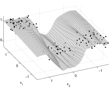
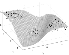
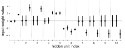
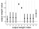
Figure 2: Case 1: An example of the overfitting of the point-estimate based ARD on a simulated data set with two relevant input features. (a) A GP model with a neural network covariance function and point-estimates for the ARD parameters. (b) An EP approximation for a neural network with 10 hidden units and independent Laplace priors with one common unknown scale parameter $\phi$ on the input weights. (c) and (d) The 95 % approximate marginal posterior probability intervals for the input weights and the output weights of the EP-based neural network.

The first case illustrates the overfitting of ARD with a similar example as presented by Qi et al. (2004). Figure 2 shows a two-dimensional regression problem with two relevant inputs $x_{1}$ and $x_{2}$. The data points are obtained from three clusters, $\{f(\mathbf{x})=1|x_{1}>0.5,x_{2}>0.5\}$, $\{f(\mathbf{x})=0|0.5>x_{1}>-0.5,0.5>x_{2}>-0.5\}$, and $\{f(\mathbf{x})=0.8|x_{1}<-0.5,x_{2}<-0.5\}$. The noisy observations were generated according to $y=f(\mathbf{x})+\epsilon$, where $\epsilon\sim\mathcal{N}(0,0.1^{2})$. The observations can be explained by using a combination of two step functions with only either one of the input features but a more robust model can be obtained by using both of them.

Subfigure 2 shows the predictive mean of the latent function $f(\mathbf{x})$ obtained with the optimized GP-ARD solution. Input $x_{2}$ is effectively pruned out and almost a step function is obtained with respect to input $x_{1}$. Subfigure 2 shows the NN-EP solution with $K=10$ hidden units and Laplace priors with one common unknown scale parameter $\phi_{1}$ on the input weights $\mathbf{w}$. The prior for $\phi_{1}$ was defined as $\phi_{1}\sim\mathcal{N}(\mu_{\phi,0},\sigma_{\phi,0}^{2})$, where $\mu_{\phi,0}=2\log(0.1)$ and $\sigma_{\phi,0}^{2}=1.5^{2}$. The noise variance $\sigma^{2}$ was inferred using the same prior definition for both models: $\theta=\log(\sigma^{2})~{}\sim\mathcal{N}(\mu_{\theta,0},\sigma_{\theta,0}^{2})$, where $\mu_{\theta,0}=2\log(0.05)$ and $\sigma_{\theta,0}^{2}=1.5^{2}$. NN-EP produces a much smoother step function that uses both of the input features. Despite of the sparsity favoring Laplace prior, the NN-EP solution preserves the uncertainty on the input variable relevances. This shows that the approximate integration over the weight prior can help to avoid pruning out potentially relevant inputs. Subfigure 2 shows the 95% approximate marginal posterior probability intervals derived from the Gaussian approximations $q(\mathbf{w}_{k})$ with the same ordering of the weights as in vector $\mathbf{z}^{\text{T}}=[\mathbf{w}_{1}^{\text{T}},...,\mathbf{w}_{K}^{\text{T}}]$ (every third weight corresponds to the input bias term). The vertical dotted lines separate the input weights associated with the different hidden units. Subfigure 2 shows the same marginal posterior intervals for the output weights computed using $q(\mathbf{v})$. Only hidden units 5 and 6 have clearly nonzero output weights and input weights corresponding to the input variables $x_{1}$ and $x_{2}$ (see the first two weight distributions in triplets 5 and 6 in panel 2). For the other hidden units, the input weights related to $x_{1}$ and $x_{2}$ are distributed around zero and they have negligible effect on the predictions. In panel 2, the third input weight distribution corresponding to the bias term in each triplet are distributed in nonzero values for many unused hidden units but these bias effects affect only the mean level of the predictions. These nonzero bias weight values may be caused by the observations not being normalized to zero mean. The weights corresponding to hidden unit 1 differ from the other unused units, because a linear action function was assigned to it for illustration purposes. If required, a truly sparse model could be obtained by removing the unused hidden units and running additional EP iterations until convergence.

4.2 Case 2: The Effect of Sparse Priors in a Regression Problem Consisting of Additive Input Effects with Different Degree of Nonlinearity

The second case study illustrates the effects of sparse priors using a similar regression example as considered by Lampinen and Vehtari (2001). In our experiments we found two main effects from applying sparsity-promoting priors with adaptive scale parameters $\bm{\phi}=[\phi_{1},...,\phi_{L}]$ on the input-layer. Firstly, the sparse priors can help to suppress the effects of irrelevant features and protect from overfitting effects in input variable relevance determination as illustrated in Case 1 (Section 4.1). Secondly, sparsity-promoting priors with adaptive prior scale parameters $\bm{\phi}$ can mitigate the effects of unsuitable initial Gaussian prior definitions on the input layer (too large or too small initial prior variances $\tilde{\sigma}_{w,j}^{2}$, see Section 3.3.1 for discussion on the initialization). More precisely, the sparse priors with adaptive scale parameters can help to obtain better data fit and more accurate predictions by shrinking the uncertainty on the weights related to irrelevant features towards zero and by allowing the relevant input weights to gain larger values which are needed in modeling strongly nonlinear (or step) functions. Placing very large initial prior variances $\tilde{\sigma}_{w,j}^{2}$ on all weights enables the model to fit strong nonlinearities but the initial learning phase is more challenging and prone to end up in poor local minima. In this section, we demonstrate that switching to Gaussian ARD priors with adaptive scale parameter $\phi_{1},...,\phi_{d}$ after a converged EP solution is obtained with fixed Gaussian priors can reduce the effects of irrelevant features, decrease the posterior uncertainties on the predictions on $f(\mathbf{x})$, and enable the model to fit more accurately latent nonlinear effects.

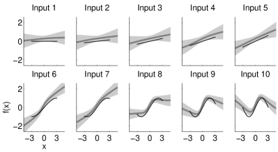
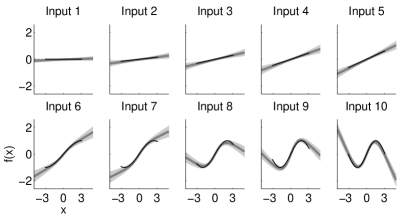
Figure 3: Case 2: An artificial regression problem where the observations are formed as a sum of additive input effects dependent on ten input features. The true additive effects are shown with black lines and the estimated mean predictions with dark grey lines. The 95% posterior predictive intervals are shaded with light grey. (a) A converged EP approximation for a neural network with ten hidden units and fixed zero-mean Gaussian priors on the input weights. (b) The resulting EP approximation when the Gaussian priors of the network in panel (a) are replaced with Gaussian ARD priors with separate scale parameters $\phi_{1},...,\phi_{d}$ for all input variables, and additional EP iterations are done until a new converged solution is obtained. Figure 4 visualizes the approximate posterior distributions of the parameters of the ARD network from panel (b).

A data set with 200 observations and ten input variables with different additive effects on the target variable was simulated. The black lines in Figure 3 show the additive effects as a function of each input variable $x_{i,j}$. The targets $y_{i}$ were calculated by summing the additive effects together and adding Gaussian noise with a standard deviation of 0.2. The first input variable is irrelevant and variables 2-5 have an increasing linear effect on the target. The effects of input variables 6-10 are increasingly nonlinear and the last three of them require at least three hidden units for explaining the observations.

Figure 3 shows the converged NN-EP solution with fixed zero-mean Gaussian priors on the input weights. The number of hidden units was set to $K=10$ and the noise variance $\sigma^{2}$ was inferred using the prior definition $\mu_{\theta,0}=2\log(0.05)$ and $\sigma_{\theta,0}^{2}=2^{2}$. The Gaussian priors were defined by initializing the prior site parameters of the input weights as $\{\tilde{\mu}_{w,j}=0,\tilde{\sigma}_{w,j}^{2}=0.4^{2}\}_{j=1}^{Kd}$. The dark grey lines illustrate the posterior mean predictions and the shaded light gray area the 95% approximate posterior predictive intervals of the latent function $f(\mathbf{x})$. The graphs are obtained by changing the value of each input in turn from $-5$ to $5$ while keeping the others fixed at zero. The training observations are obtained by sampling all input variables linearly from the interval $x_{i,j}\in[-\pi,\pi]$. Panel 3 shows the resulting NN-EP solution when the Gaussian priors of the network in panel 3 are replaced with Gaussian ARD priors with adaptive scale parameter $\phi_{1},...,\phi_{d}$ and additional EP iterations are done until convergence. Prior distributions for the scale parameters were defined as $\phi_{l}\sim\mathcal{N}(\mu_{\phi,0},\sigma_{\phi,0}^{2})$, where $\mu_{\phi,0}=2\log(0.01)$ and $\sigma_{\phi,0}^{2}=2.5^{2}$. This prior definitions favors small input variances close to $0.01$ but enables also larger values around one. It should be noted that the actual variance parameters $\tilde{\sigma}_{w,j}^{2}$ of the prior site approximations can attain much larger values from the EP updates.

With the Gaussian priors (Figure 3), the predictions do not capture the nonlinear effects very accurately and the model produces a small nonzero effect on the irrelevant input 1. Applying the ARD priors (Figure 3) with additional iterations produces clearly more accurate predictions on the latent input effects and effectively removes the predictive effect of input 1. The overall approximate posterior uncertainties on the latent function $f(\mathbf{x})$ are also smaller compared with the initial Gaussian priors. We should note that the result of panel (a) depends on the initial Gaussian prior definitions and choosing a smaller $\tilde{\sigma}_{w,j}^{2}=0.2^{2}$ or optimizing it could give more accurate predictions compared with the solution visualized in panel (a).

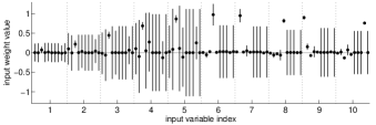
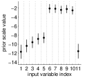
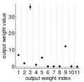
Figure 4: Case 2: Visualization of the model parameters related to the artificial regression problem shown in Figure 3. Panels (a), (b), and (c) show the 95% marginal posterior credible intervals for the input weights $\mathbf{w}$, the scale parameters $\phi_{1},...,\phi_{d}$, and the output weights $\mathbf{v}$ of the neural network with Gaussian ARD priors from Figure 3. In panel (a) the input weights associated with each additive input effect (1-10) are grouped together (the bias terms are not shown). The weight distributions related to the linear input effects 1–5 are much smaller compared with the nonlinear effects 6–10, which is why they are scaled by 40 for better illustration in panel (a).

Figure 4 shows the 95% posterior credible intervals for the input weights $\mathbf{w}$ (a), the prior scale parameters $\phi_{1},...,\phi_{d}$ (b), and the output weights $\mathbf{v}$ (c) of the NN-EP approximation with ARD priors visualized in Figure 3. In panel 4 the input weights from the different hidden units are grouped together according to the different additive input effects 1–10, and the weights related to the linear effects 1–5 are scaled by 40 for illustration purposes, because they are much smaller compared with the weights associated with the nonlinear input effects 6–10. From panels 4 and 4 we see that only hidden units are 1–5 and 9 have clearly non-zero effect on the predictions. The linear effects of inputs 1–5 are modeled by unit 3 that has very small but clearly nonzero input weights in panel 4 and a very large output weight in panel 4. The input weights related to the irrelevant input 1 are all zero in the 95% posterior confidence level. By comparing panels 4 and 4 we can also see that hidden units 1, 2, 4, 5, and 9 are most probably responsible for modeling the nonlinear input effects 6-7 because of large input weights values. Panel 4 gives further evidence on this interpretation because the scale parameters associated with the nonlinear input effects 6–10 are clearly larger compared to effects 1–5. The scale parameters associated with the linear input effects 1–5 increase steadily as the magnitudes of the true effects increase. These results are congruent with the findings of Lampinen and Vehtari (2001) who showed by MCMC experiments that with MLP models the magnitudes of the ARD parameters and the associated input weights also reflect the degree of nonlinearity associated with the latent input effects, not only the relevance of the input features.

4.3 Case 3: Comparison of a Finite vs. Infinite Network with Observations from a Latent Function with a Discontinuity

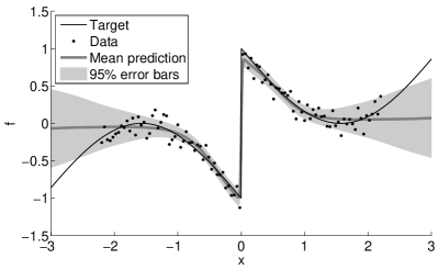
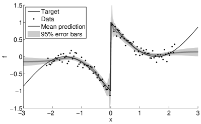
Figure 5: Case 3: An artificial regression problem consisting of noisy observations (black dots) generated from a latent function (black lines) that has a discontinuity at zero. Panel (a) shows the mean predictions (dark grey line) and the 95% credible intervals (light gray shaded area) obtained using the proposed EP approach for a NN with ten hidden units and Laplace priors with one common scale parameter $\phi$ on the input weights. Panel (b) visualizes the corresponding predictive distribution obtained using a GP with a neural network covariance function.

The third case study compares the performance of the finite NN-EP network with an infinite GP network in a one-dimensional regression problem with a strong discontinuity. Figure 5 shows the true underlying function (black lines) that has a discontinuity at zero together with the noisy observations (black dots). Panel 5 shows the predictive distributions obtained using NN-EP with ten hidden units ($K=10$) and Laplace priors with one common scale parameter $\phi$. The prior distribution for the scale parameter was defined with $\mu_{\phi,0}=2\log(0.01)$ and $\sigma_{\phi,0}^{2}=2.5^{2}$, and the noise variance $\sigma^{2}$ was inferred from the data using the prior definition $\mu_{\theta,0}=2\log(0.05)$ and $\sigma_{\theta,0}^{2}=2^{2}$. Panel 3 shows the corresponding predictions obtained using a GP with a neural network covariance function. With the GP network the noise variance was optimized together with the other hyperparameters using the marginal likelihood. The finite NN-EP network explains the discontinuity with a slightly smoother step compared to infinite GP network, but the GP mean estimate shows fluctuations near the discontinuity. It seems that the infinite GP network fits more strongly to individual observations near the discontinuity. This shows that a flexible parametric model with a limited complexity may generalize better with finite amount of observations even though the GP model includes the correct solution a priori. This is in accordance with the results described by Winther (2001).

4.4 Predictive Comparisons with Real World Data

In this section the predictive performance of NN-EP is compared to three other nonlinear regression methods using the following real-world data sets: the concrete quality data (Concrete) analyzed by Lampinen and Vehtari (2001), the Boston housing data (Housing) and the unnormalized Communities and Crime data (Crime) that can be obtained from the UCI data repository (Frank and Asuncion, 2010), and the robot arm data (Kin40k) utilized by Schwaighofer and Tresp (2003). The number of observations $n$ and the number of input features $d$ are shown in Table 1 for each data set. The Kin40k includes originally only 8 input features but we added 92 irrelevant uniformly sampled random inputs to create a challenging feature selection problem. The columns of the input matrices $\mathbf{X}$ and the output vectors $\mathbf{y}$ were normalized to zero mean and unit variance for all methods. The predictive performance of the models was measured using the log predictive densities and the squared errors evaluated with separate test data. We used 10-fold cross-validation with the Housing, Concrete, and Crime data, whereas with Kin40k we chose randomly 5000 data points for training and used the remaining observations for validation.

The proposed NN-EP solution was computed using two alternative prior definitions: Laplace priors with one common scale parameter $\phi$ (NN-EP-LA), and Gaussian ARD priors with separate scale parameters $\phi_{1},...,\phi_{d}$ for all inputs including the input bias terms (NN-EP-ARD). With both prior frameworks, the hyperpriors for the scale parameters were defined as $\phi_{l}\sim\mathcal{N}(\mu_{\phi,0},\sigma_{\phi,0}^{2})$, where $\mu_{\phi,0}=2\log(0.01)$ and $\sigma_{\phi,0}^{2}=2.5^{2}$. This definition encourages small input weight variances (around $0.01^{2}$) but enables also large input weight values if required for strong nonlinearities assuming the input variables are scaled to unit variance. The noise level $\theta=\log(\sigma^{2})$ was inferred from data with a prior distribution defined by $\mu_{\theta,0}=2\log(0.01)$ and $\sigma_{\theta,0}^{2}=2^{2}$, which is a sufficiently flexible prior when the output variables $\mathbf{y}$ are scaled to unit variance. The methods used for comparison include an MCMC-based MLP network with ARD priors (NN-MC) and two GPs with a neural network covariance function: one with common variance parameter for all inputs (GP), and another with separate variance hyperparameters for all inputs (GP-ARD). With both GP models the hyperparameters were estimated by gradient-based optimization of the analytically tractable marginal likelihood (Rasmussen and Williams, 2006). For NN-MC and NN-EP, we set the number of hidden units to $K=10$ with the Housing, Concrete, and Crime data sets. With the Kin40k data, we set $K=30$ because $n$ is large and fewer units were found to produce clearly worse data fits.

Table 1 summarizes the means (mean) and standard deviations (std) of the log predictive densities (LPDs) and the squared errors (SEs). Because the distributions of the LPD values are heavily skewed towards negative values, we summarize also the lower 1% percentiles (prct 1%). Similarly, because the SE values are skewed towards positive values we summarize also the 99% percentiles (prct 99%). These additional measures describe the quality of the worst case predictions of the methods. Table 1 summarizes also the average relative CPU times (cputime) required for parameter estimation and predictions using MATLAB implementations. The GP models were implemented using the GPstuff toolbox and NN-MC was implemented using the MCMCstuff toolbox. The CPU times were averaged over the CV-folds and scaled so that the relative cost for NN-EP is one. These running time measures are highly dependent on the implementation, the tolerance levels in optimization and iterative algorithms, and the number of posterior draws, and therefore they are reported only to summarize the main properties regarding the scalability of the different methods. When assessing the results with respect to the Housing and Concrete data sets, it is worth noting that there is evidence that an outlier-robust observation model is beneficial over the Gaussian model used in this comparison with both data sets (Jylänki et al., 2011).

Table 1: A predictive assesment of the proposed EP approach for neural networks with two different prior definitions: Laplace priors with one common scale parameter $\phi$ (NN-EP-LA) and Gaussian ARD priors with separate scale parameters $\phi_{1},...,\phi_{d}$ for all inputs (NN-EP-ARD). The methods used for comparison include a neural network with ARD priors inferred using MCMC (NN-MC), and two GPs with a neural network covariance: one with a common variance hyperparameter for all inputs (GP), and another with separate variance hyperparameters for all inputs (GP-ARD). The log predictive densities are summarized with their means, standard deviations (std), and lower 1% percentiles (prct 1%). The squared errors are summarized with their means, standard deviations (std), and upper 99% percentiles (prct 99%).

Housing	log predictive density (LPD)			squared error (SE)
($n$=506, $d$=13)	mean	std	prct 1%	mean	std	prct 99%	cputime
NN-EP-LA	-0.44	1.64	-7.55	0.15	0.45	2.42	1.0
NN-EP-ARD	-0.50	1.66	-6.31	0.17	0.49	1.60	1.0
NN-MC	-0.08	1.17	-4.54	0.11	0.50	1.18	110.5
GP	-0.29	2.35	-7.57	0.13	0.53	1.98	0.3
GP-ARD	-0.20	2.00	-10.71	0.10	0.37	1.53	1.0
Concrete ($n$=215, $d$=27)
NN-EP-LA	0.18	0.85	-3.05	0.05	0.08	0.30	1.0
NN-EP-ARD	0.05	1.03	-4.61	0.05	0.11	0.57	0.8
NN-MC	0.22	1.52	-3.62	0.04	0.08	0.28	103.0
GP	-0.07	1.70	-5.12	0.06	0.11	0.66	0.03
GP-ARD	0.15	1.98	-4.23	0.04	0.08	0.28	0.6
Crime ($n$=1993, $d$=102)
NN-EP-LA	-0.83	0.89	-4.64	0.31	0.55	2.60	1.0
NN-EP-ARD	-0.84	0.89	-4.81	0.31	0.55	2.75	0.2
NN-MC	-0.80	0.93	-4.81	0.29	0.53	2.60	19.8
GP	-0.81	0.91	-4.80	0.30	0.54	2.69	0.2
GP-ARD	-0.81	1.01	-5.49	0.30	0.55	2.75	4.4
Kin40k ($n$=5000, $d$=100)
NN-EP-LA	-0.59	0.89	-4.27	0.19	0.29	1.38	1.0
NN-EP-ARD	0.27	1.19	-4.63	0.03	0.08	0.37	0.9
NN-MC	0.49	1.51	-5.37	0.02	0.07	0.26	48.7
GP	-1.15	0.72	-4.18	0.58	0.83	4.06	0.5
GP-ARD	0.64	1.11	-3.90	0.02	0.05	0.24	32.3

Table1 shows that NN-EP-LA performs slightly better compared to NN-EP-ARD in all data sets except in Kin40k, where NN-EP-ARD gives clearly better results. The main reason for this is probably the stronger sparsity of the NN-EP-ARD solutions: In Kin40k data there are a large number truly irrelevant features that should be completely pruned out of the model, whereas with the other data sets most features have probably some relevance for predictions or at least they are not generated in a completely random manner. Further evidence for this is given by the clearly better performance of GP-ARD over GP with the Kin40k data.

If the mean log predictive densities (MLPDs) are considered, the NN-MC approach based on a finite network performs best in all data sets except with Kin40k, where the infinite GP-ARD network is slightly better. The main reason for this is probably the strong nonlinearity of the true latent mapping, which requires a large number of hidden units, and consequently the infinite GP network with ARD priors gives very accurate predictions. In pair-wise comparisons the differences in MLPDs are significant in 95% posterior confidence level only with Housing and Kin40k data sets. In terms of mean squared errors (MSEs), GP-ARD is best in all data sets except Crime, but with 95% confidence level the pair-wise differences are significant only with the Kin40k data. With the Kin40k data, the performance of NN-MC could probably be improved by increasing $K$ or drawing more posterior samples, because learning the nonlinear mapping with a large number of unknown parameters and potentially multimodal posterior distribution may require a very large number of posterior draws.

When compared with NN-MC and GP-ARD, NN-EP gives slightly worse MLPD scores with all data sets except with Concrete. The pair-wise differences in MLPDs are significant with 95% confidence level in all cases except with the Concrete data. In terms of MSE scores, NN-EP is also slightly but significantly worse with 95% confidence level in all data sets. By inspecting the std:s and 1% percentiles of the LPDs, it can be seen that NN-EP achieves better or comparable worst case performance when compared to GP-ARD. In other words, NN-EP seems to make more cautions predictions by producing less very high or very low LPD values. One possible explanation for this behavior is that it might be an inherent property of the chosen approximation. Approximating the possibly multimodal tilted distribution $\hat{p}(h_{i,k})$, where one mode is near the cavity distribution $q_{-i}(h_{i,k})$ and another at the values of $h_{i,k}$ giving the best fit for $y_{i}$, with an unimodal Gaussian approximation as described in Appendix C, may lead to reduced fit to individual observations. Another possibility is that the EP-iterations have converged into a suboptimal stationary solution or the maximum number of iterations has been exceeded. Doing more iterations or using an alternative non-zero initialization for the input-layer weights might result in better data fit. The second possibility is supported by the generally acknowledged benefits from different initializations, for example, the unsupervised schemes discussed by Erhan et al. (2010), and our experiments using the Kin40k data without the extra random inputs. We found that initializing the location parameters $\tilde{\mu}_{v,k}$ and $\tilde{\mu}_{w,j}$ of the prior site approximations (13) and (14) using a gradient-based MAP estimate of the weights $\mathbf{w}$ and $\mathbf{v}$, and relaxing the prior site approximations after initial iterations using the proposed EP framework, can result in better MSE and MLPD scores. However, such alternative initialization schemes were left out of these experiments, because our aim was to test how good performance could be obtained using only the EP algorithm with the zero initialization described in Section 3.3.1.

The CPU times of Table 1 indicate that with small $n$ the computational cost of NN-EP is larger compared to GP-ARD, which requires only one $\mathcal{O}(n^{3})$ Cholesky decomposition per analytically tractable marginal likelihood evaluation. However, as $n$ increases GP-ARD becomes slower, which is why several different sparse approximation schemes have been proposed (see, e.g, Rasmussen and Williams, 2006). Furthermore, assuming a non-Gaussian observation model, such as the binary probit classification model, GP or GP-ARD would require several $\mathcal{O}(n^{3})$ iterations to form Laplace or EP approximations for the marginal likelihood at each hyperparameter configuration. With NN-EP, probit or Gaussian mixture models could be used without additional computations. The computational cost of NN-EP increases linearly with $n$ and $K$, but as $d$ increases the posterior updates of $q(\mathbf{w}_{k})$, which scale as $\mathcal{O}(Kd^{3})$, become more demanding. The results of Table 1 were generated using a sequential scheme for updating $q(\mathbf{w}_{k})$ (see Algorithm 1), which can be seen as larger computational costs with respect to NN-MC with the Crime and Kin40k data sets. One option with larger $d$ is to use parallel EP updates, but this may require more damping or better initialization for the input weight approximations. Another possibility would be to use fully factorized posterior approximations in place of $q(\mathbf{w}_{k})$, or to assign different overlapping subgroups of the input features into the different hidden units and to place hierarchical prior scale parameters between the groups.

5 Discussion

In this article, we have described how approximate inference using EP can be carried out with a two-layer NN model structure with sparse hierarchical priors on the network weights, resulting in a novel method for nonlinear regression problems.

We have described a computationally efficient EP algorithm that utilizes independent approximations for the weights associated with the different hidden units and layers to achieve computational complexity scaling similar to an ensemble of $K$ sparse linear models. More generally, our approach can be regarded as a non-linear adaptation of the various EP methods proposed for sparse linear regression models. This is achieved by constructing a factorized Gaussian approximation for the posterior distribution resulting from the nonlinear MLP model structure with a linear input layer, and adapting the algorithms proposed for sparse linear models separately on the independent Gaussian approximations for each hidden unit. Because of the structure of the approximation, all existing methodology presented for facilitating the computations in sparse linear models can be applied on the hidden unit approximations separately. We have also introduced an EP framework that enables definition of flexible hierarchial priors using higher level scale parameters that are shared by a group of independent linear models (in our case the hidden units). The proposed EP approach enables efficient approximate integration over these scale parameters simultaneously with the coefficients of the linear models. We used this framework for inferring the common scale parameter of Laplace priors assigned on the input weights, and to implement Gaussian ARD priors for the input-layer. In this article, we have focused on the Gaussian observation model, but the method can be readily extended to others as well (e.g., binary probit classification and robust regression with Gaussian mixture models).

Using simple artificial examples we demonstrated several desirable characteristics of our approach. The sparsity promoting priors can be used to suppress the confounding predictive influences of possibly irrelevant features without the potential risk of overfitting associated with point-estimate based ARD priors. More precisely, the approximate integration over the posterior uncertainty helps to avoid pruning out potentially relevant features in cases with large uncertainty on the input relevances. Albeit more challenging to estimate, the finite parametric model enables a posteriori inspection of the model structure and feature relevances using the hyperparameter and weight approximations. Furthermore, the parametric model structure can also be used to construct more restricted models by assigning different input variables into different hidden units, grouping the inputs using the hierarchical scale priors, using different nonlinear activation functions for the different hidden units, or using fixed interaction terms dependent on certain hidden units as inputs for the output-layer.

In deriving the EP algorithm, we have also described different computational techniques that could be useful in other models and approximation methods. These include the EP approximation for the hierarchical priors on the scale parameters of the weights that could be useful in combining sparse linear models associated with different subjects or measurement instances, the noise estimation framework that could be used for estimating the likelihood parameters in sparse linear models or approximate Gaussian filtering methods, and the proposed approach for approximating the tilted distributions of the hidden unit activations that could be useful in forming EP approximations for observation models involving sums of nonlinear functions taken from random variables with factorized Gaussian posterior approximations.

Acknowledgments

This research was partially funded by the Academy of Finland (grant 218248).

A Cavity Distributions with the Factorized Approximation

Assuming the factorized approximation of equation (20) for $q(\mathbf{z})$, and applying the transformation $\mathbf{h}_{i}=\tilde{\mathbf{x}}_{i}^{\text{T}}\mathbf{w}$ on (23) results in the following cavity distribution for $\mathbf{h}_{i}$: $q_{-i}(\mathbf{h}_{i})=\prod_{k}\mathcal{N}(h_{i,k}|m_{-i,k},V_{-i,k})$. The scalar cavity means and variances are given by

$$V_{-i,k} =(V_{i,k}^{-1}-\eta\tilde{\tau}_{i,k})^{-1}$$

$$m_{-i,k} =V_{-i,k}(V_{i,k}^{-1}m_{i,k}-\eta\tilde{\nu}_{i,k}),$$ (31)

where the mean and variance of $h_{i,k}$ under the current approximation (21) are denoted with $m_{i,k}=\mathbf{x}_{i}^{\text{T}}\bm{\mu}_{\mathbf{w}_{k}}$ and $V_{i,k}=\mathbf{x}_{i}^{\text{T}}\bm{\Sigma}_{\mathbf{w}_{k}}\mathbf{x}_{i}$, respectively. Using (22) and (23) the $i$:th cavity distribution for $\mathbf{v}$ can be written as $q_{-i}(\mathbf{v})=\mathcal{N}(\mathbf{v}|\bm{\mu}_{-i},\bm{\Sigma}_{-i})$ and the cavity mean and covariance are given by

$$\bm{\Sigma}_{-i} =\bm{\Sigma}_{\mathbf{v}}+\bm{\Sigma}_{\mathbf{v}}\tilde{\bm{\alpha}}_{i}s^{-1}\tilde{\bm{\alpha}}_{i}^{\text{T}}\bm{\Sigma}_{\mathbf{v}}$$

$$\bm{\mu}_{-i} =\mathbf{a}+\bm{\Sigma}_{\mathbf{v}}\tilde{\bm{\alpha}}_{i}s^{-1}\tilde{\bm{\alpha}}_{i}^{\text{T}}\mathbf{a},$$ (32)

where $s=\eta^{-1}-\tilde{\bm{\alpha}}_{i}^{\text{T}}\bm{\Sigma}_{\mathbf{w}}\tilde{\bm{\alpha}}_{i}$ and $\mathbf{a}=\bm{\mu}_{\mathbf{v}}-\eta\bm{\Sigma}_{\mathbf{v}}\tilde{\bm{\beta}}_{i}$. Using (A) and (A) the cavity evaluations can be implemented efficiently: for the input weights $\mathbf{w}_{k}$ only scalar moments of $h_{i,k}$ need to be determined, and for the output weights $\mathbf{v}$ rank-one matrix updates are required. The cavity computations for the noise level term approximations (12) and the weight prior term approximations (13, 14) require only manipulation of univariate Gaussian distributions and can be implemented similarly as in (A).

B Tilted Moments for the Output Weights

To obtain the desired site approximation structure (19) and closed form expressions for the the corresponding site parameters ($\tilde{\bm{\tau}}_{i}$, $\tilde{\bm{\nu}}_{i}$, $\tilde{\bm{\alpha}}_{i}$, and $\tilde{\bm{\beta}}_{i}$) satisfying the moment matching condition (25) we need to form suitable approximations for the marginal means and covariances of $h_{i,k}$ and $\mathbf{v}$ resulting from the tilted distribution $\eqref{eq_EP_tilted}$. We start by assuming the noise level $\theta$ known and extend the presented approach for approximate integration over $q_{-i}(\theta)$ later.

We first consider an approximate scheme which has already been utilized in the unscented Kalman filtering framework for inferring the weights of a neural network (Wan and van der Merwe, 2000). Adopting the approach to our setting, first a cavity-predictive joint Gaussian approximation is formed for the random vector $[\mathbf{u}_{i}^{\text{T}},\tilde{y}_{i}]^{\text{T}}=[\mathbf{h}_{i}^{\text{T}},\mathbf{v}^{\text{T}},\tilde{y}_{i}]^{\text{T}}$, which is distributed according to $q(\mathbf{h}_{i},\mathbf{v},\tilde{y}_{i}|\theta)\propto p(\tilde{y}_{i}|f_{i},\theta)^{\eta}q_{-i}(\mathbf{h}_{i},\mathbf{v})$. This is done by approximating the central moments $\operatorname{E}(\tilde{y}_{i}|\theta)$, $\operatorname{Var}(\tilde{y}_{i}|\theta)$, $\operatorname{Cov}(\mathbf{h}_{i},\tilde{y}_{i}|\theta)$, and $\operatorname{Cov}(\mathbf{v},\tilde{y}_{i}|\theta)$ using the unscented transform. Approximations for the mean and covariance of the tilted distribution (24) can now be determined by conditioning on $\tilde{y}_{i}$ in the joint Gaussian approximation of $[\mathbf{u}_{i}^{\text{T}},\tilde{y}_{i}]^{\text{T}}$ to obtain $\operatorname{E}(\mathbf{u}_{i}|\tilde{y}_{i},\theta)$ and $\operatorname{Cov}(\mathbf{u}_{i}|\tilde{y}_{i},\theta)$, and plugging in the observation $y_{i}$. In our experiments, this approach was found sufficiently accurate for approximating the moments of $\mathbf{v}$, which is probably explained by the conditional linear dependence of $f_{i}$ on $\mathbf{v}$ in the observation model. Thus, we approximate the marginal tilted distribution of $\mathbf{v}$ with $\hat{p}_{i}(\mathbf{v}|\theta)\approx\mathcal{N}(\hat{\bm{\mu}}_{i}(\theta),\hat{\bm{\Sigma}}_{i}(\theta))$, where

$$\hat{\bm{\mu}}_{i}(\theta) =\bm{\mu}_{-i}+\bm{\Sigma}_{\mathbf{v},f_{i}}V_{y_{i}}^{-1}(y_{i}-m_{f_{i}})$$

$$\hat{\bm{\Sigma}}_{i}(\theta) =\bm{\Sigma}_{-i}-\bm{\Sigma}_{\mathbf{v},f_{i}}V_{y_{i}}^{-1}\bm{\Sigma}_{\mathbf{v},f_{i}}^{\text{T}},$$ (33)

and $V_{y_{i}}=V_{f_{i}}+\eta^{-1}\exp(\theta)$. Here we have defined the required cavity predictive moments in terms of $f_{i}=\mathbf{v}^{\text{T}}\mathbf{g}(\mathbf{h}_{i})$ instead of $\tilde{y}_{i}$ to facilitate the upcoming approximate integration over $q_{-i}(\theta)$, and assuming the factorized posterior approximation (20), these central moments can be written as

$$m_{f_{i}} =\operatorname{E}(f_{i})=\bm{\mu}_{-i}^{\text{T}}\mathbf{m}_{\mathbf{g}_{i}}$$

$$V_{f_{i}} =\operatorname{Var}(f_{i})=\mathbf{m}_{\mathbf{g}_{i}}^{\text{T}}\bm{\Sigma}_{-i}\mathbf{m}_{\mathbf{g}_{i}}+\mathbf{V}_{g_{i}}^{\text{T}}(\textrm{diag}(\bm{\Sigma}_{-i})+\bm{\mu}_{-i}\circ\bm{\mu}_{-i})$$

$$\bm{\Sigma}_{\mathbf{v},f_{i}} =\operatorname{Cov}(\mathbf{v},f_{i})=\bm{\Sigma}_{-i}\mathbf{m}_{\mathbf{g}_{i}},$$ (34)

where $\circ$ denotes the element-wise matrix product, and the $(K+1)\times 1$ vectors $\mathbf{m}_{\mathbf{g}_{i}}=\operatorname{E}(\mathbf{g}(\mathbf{h}_{i}))$ and $\mathbf{V}_{\mathbf{g}_{i}}=\operatorname{Var}(\mathbf{g}(\mathbf{h}_{i}))$ are formed by computing the means and variances from each component of $\mathbf{g}(\mathbf{h}_{i})$ with respect to $q_{-i}(\mathbf{h}_{i})$ defined in (A). Note that the last elements of $\mathbf{m}_{\mathbf{g}_{i}}$ and $\mathbf{V}_{\mathbf{g}_{i}}$ are one and zero corresponding to the output bias term $v_{0}$.

With the activation function (2) the mean $\mathbf{m}_{\mathbf{g}_{i}}$ can be computed analytically as

$$\operatorname{E}(g(h_{i,k}))=2K^{-1/2}\left(\Phi\left(m_{-i,k}(1+V_{-i,k})^{-1/2}\right)-0.5\right),$$

and for computing the variance $\mathbf{V}_{\mathbf{g}_{i}}$ the following integral has to be evaluated numerically

$$\operatorname{Var}(g(h_{i,k}))=2(K\pi)^{-1}\int_{0}^{\sin^{-1}(\rho)}\exp\left(-\frac{m_{-i,k}^{2}}{(1+V_{-i,k})(1+\sin(x))}\right)dx,$$

where $\rho=V_{-i,k}(1+V_{-i,k})^{-1}$. Other activation functions could be incorporated by using only one-dimensional numerical quadratures whereas with the full posterior couplings (16) $K$-dimensional numerical integrations would be required to approximate $m_{f_{i}}$, $V_{f_{i}}$, and $\bm{\Sigma}_{\mathbf{v},f_{i}}$.

C Tilted Moments for the Hidden Unit Activations

The challenge in approximating the mean and variance of $\hat{p}_{i}(h_{i,k})$ is that this marginal density can have multiple distinct modes, one related to the cavity distribution $q_{-i}(\mathbf{h}_{i})$ and another related to the likelihood $p(y_{i}|\mathbf{v}^{\text{T}}\mathbf{g}(\mathbf{h}_{i}),\theta)$, that is, to the values of $h_{i,k}$ that give better fit for the left-out observation $y_{i}$. In our numerical experiments, the previously described simple approach based on a joint Gaussian approximation for $[\mathbf{h}_{i}^{\text{T}},\mathbf{v}^{\text{T}}f_{i}]$ was found to underestimate the marginal probability mass of the latter mode related to $y_{i}$ especially in cases where the modes were clearly separated from each other. This problem was found to be mitigated by decreasing $\eta$, which probably stems from leaving a fraction of the old site approximation $\tilde{t}_{\mathbf{z},i}$ from the previous iteration in the approximation that in turn shifts the cavity towards the observation $y_{i}$. With some difficult data sets, $\eta$-values as small as 0.5 were found necessary for obtaining a good data fit but usually this also required more iterations for achieving convergence compared to larger values of $\eta$.

To form a robust approximation for the marginal tilted distributions of the hidden unit activations $h_{i,k}$ also in case of multimodalities, we propose an alternative approximate method that enables numerical integration over $\hat{p}_{i}(h_{i,k}|\theta)$ using one-dimensional quadratures. We aim to explore numerically the effect of each hidden activation $h_{i,k}$ on the tilted distributions $\hat{p}_{i}(\mathbf{h}_{i},\mathbf{v}|\theta)\propto\mathcal{N}(y_{i}|\mathbf{v}^{\text{T}}\mathbf{g}(\mathbf{h}_{i}),\exp(\theta))^{\eta}q_{-i}(\mathbf{h}_{i})q_{-i}(\mathbf{v})$ when all other activations $\mathbf{h}_{i,-k}$ and the weights $\mathbf{v}$ are averaged out. To approximate the marginalization over $\mathbf{h}_{i,-k}$ and $\mathbf{v}$ we approximate $q_{-i}(f_{i}|h_{i,k})$, that is, the cavity distribution of $f_{i}$ resulting from $q_{-i}(\mathbf{h}_{i})q_{-i}(\mathbf{v})$ by conditioning on $h_{i,k}$, with a univariate Gaussian given by

$$q_{-i}(f_{i}|h_{i,k})\approx\mathcal{N}\left(f_{i}|m(h_{i,k}),V(h_{i,k})\right),$$ (35)

where $m(h_{i,k})$ and $V(h_{i,k})$ denote the mean and variance of $f_{i}$ computed with respect to $q_{-i}(\mathbf{h}_{i,-k},\mathbf{v})=q_{-i}(\mathbf{h}_{i,-k})q_{-i}(\mathbf{v})$. The required conditional moments $m(h_{i,k})$ and $V(h_{i,k})$ can be calculated using equation (B) by modifying the $k$:th element of $\mathbf{m}_{\mathbf{g}_{i}}$ and $\mathbf{V}_{\mathbf{g}_{i}}$ corresponding to the known values of $h_{i,k}$, that is, $[\mathbf{m}_{\mathbf{g}_{i}}]_{k}=g(h_{i,k})$ and $[\mathbf{V}_{\mathbf{g}_{i}}]_{k}=0$. Note that the possible numerical integrations for determining $\operatorname{E}(\mathbf{g}(\mathbf{h}_{i}))$ and $\operatorname{Var}(\mathbf{g}(\mathbf{h}_{i}))$ need to be computed only once for each site update and only the terms dependent on $\mathbf{m}_{\mathbf{g}_{i},k}$ have to be re-evaluated for each value of $h_{i,k}$. The approximation (35) can be justified using the central limit theorem according to which the distribution of the sum in $f_{i}=\sum_{k^{\prime}}v_{k^{\prime}}g(h_{i,k^{\prime}})+v_{0}$ given $h_{i,k}$ approaches a normal distribution as $K$ increases.

Using equation (35), we can write the following approximation for the marginal tilted distribution of $h_{i,k}$:

$$\hat{p}_{i}(h_{i,k}|\theta) \propto\int\mathcal{N}(y_{i}|\mathbf{v}_{-k}^{\text{T}}\mathbf{g}(\mathbf{h}_{i,-k})+v_{k}h_{i,k},\exp(\theta))^{\eta}q_{-i}(\mathbf{v})\prod_{k^{\prime}=1}^{K}q_{-i}(h_{i,k^{\prime}})d\mathbf{v}d\mathbf{h}_{i,-k}$$

$$=\int\mathcal{N}\left(y_{i}|f_{i},\exp(\theta)\right)^{\eta}q_{-i}\left(f_{i}|h_{i,k})\right)q_{-i}(h_{i,k})df_{i}$$

$$\approx Z(\theta)\mathcal{N}\left(y_{i}|m(h_{i,k}),V(h_{i,k})+\eta^{-1}\exp(\theta)\right)q_{-i}(h_{i,k})$$

$$\approx\hat{Z}_{i,k}(\theta)\mathcal{N}\big{(}h_{i,k}|\hat{m}_{i,k}(\theta),\hat{V}_{i,k}(\theta)\big{)},$$ (36)

where all output weights excluding $v_{k}$ are denoted by $\mathbf{v}_{-k}$ and $\hat{Z}_{i,k}(\theta)$ is a normalizing constant. In the last step we have substituted approximation (35) and carried out the integration over $f_{i}$ analytically to give $Z(\theta)=(2\pi\exp(\theta))^{(1-\eta)/2}\eta^{-1/2}$. Approximation (C) enables numerical inspection for the possible multimodality of $\hat{p}_{i}(h_{i,k}|\theta)$, and the conditional tilted mean $\hat{m}_{i,k}(\theta)$ and variance $\hat{V}_{i,k}(\theta)$ can be determined using a numerical quadrature. Compared with the simple approach described in Appendix B, equation (C) results in more accurate tilted mean estimates in multimodal cases.

D Tilted Moments with Unknown Noise Level

If the noise level $\theta$ is assumed unknown and estimated using the EP, the marginal mean $\hat{\mu}_{\theta,i}$ and variance $\hat{\sigma}_{\theta,i}^{2}$ can be approximated with a similar approach as was done for $h_{i,k}$ in Appendix C. We approximate first the cavity distribution of $f_{i}$ with $q_{-i}(f_{i}|\theta)\approx\mathcal{N}(y_{i}|m_{f_{i}},V_{f_{i}})$, where the mean and variance are computed using (B). Then, assuming a Gaussian observation model, we can integrate analytically over $f_{i}$ to obtain a numerical approximation for the tilted distribution of $\theta$:

$$\hat{p}_{i}(\theta) \propto\int\mathcal{N}(y_{i}|\mathbf{v}^{\text{T}}\mathbf{g}(\mathbf{h}_{i}),\exp(\theta))^{\eta}q_{-i}(\mathbf{v})q_{-i}(\mathbf{h}_{i})q_{-i}(\theta)d\mathbf{v}d\mathbf{h}_{i}$$

$$=\int\mathcal{N}\left(y_{i}|f_{i},\exp(\theta)\right)^{\eta}q_{-i}(f_{i})q_{-i}(\theta)df_{i}$$

$$\approx Z(\theta)\mathcal{N}\left(y_{i}|m_{f_{i}},V_{f_{i}}+\eta^{-1}\exp(\theta)\right)q_{-i}(\theta)\approx\hat{Z}_{i}\mathcal{N}(\theta|\hat{\mu}_{\theta,i},\hat{\sigma}^{2}_{\theta,i}),$$ (37)

where $Z(\theta)=(2\pi\exp(\theta))^{(1-\eta)/2}\eta^{-1/2}$, and $\hat{Z}_{i}$ is an approximation for the normalization term of the tilted distribution (24). Using equation (D) the approximate mean $\hat{\mu}_{\theta,i}$, variance $\hat{\sigma}_{\theta,i}^{2}$, and normalization term $\hat{Z}_{i}$ can be calculated with a numerical quadrature, and if $\theta$ is known or fixed, the normalization term can by approximated with $\hat{Z}_{i}(\theta)=Z(\theta)\mathcal{N}\left(y_{i}|m_{f_{i}},V_{f_{i}}+\eta^{-1}\exp(\theta)\right)$.

To approximate the marginal means and covariances of $\mathbf{v}$ and $h_{i,k}$ with unknown $\theta$ the conditional approximations of equations (B) and (C) have to be integrated over $\hat{q}_{i}(\theta)=\hat{Z}_{i}^{-1}\hat{Z}_{i}(\theta)q_{-i}(\theta)\approx\hat{p}_{i}(\theta)$ because we have $\hat{p}_{i}(\mathbf{h}_{i},\mathbf{v},\theta)\approx\hat{Z}_{i}^{-1}\hat{p}_{i}(\mathbf{h}_{i},\mathbf{v}|\theta)\hat{Z}_{i}(\theta)q_{-i}(\theta)$ according to (D). In case of the simple joint Gaussian approximation for $\mathbf{v}$ we can write

$$\hat{\bm{\mu}}_{i}=\operatorname{E}_{\hat{p}_{i}(\mathbf{v})}(\mathbf{v}) =\operatorname{E}_{\hat{p}_{i}(\theta)}\big{(}\operatorname{E}_{\hat{p}_{i}(\mathbf{v}|\theta)}(\mathbf{v}|\theta)\big{)}\approx\operatorname{E}_{\hat{q}_{i}(\theta)}(\hat{\bm{\mu}}_{i}(\theta))$$

$$=\bm{\mu}_{-i}+\bm{\Sigma}_{\mathbf{v},f_{i}}\operatorname{E}_{\hat{q}_{i}(\theta)}\big{(}V_{y_{i}}^{-1}\big{)}(y_{i}-m_{f_{i}}),$$ (38)

where the conditional mean of $\mathbf{v}$ with respect to $\hat{p}_{i}(\mathbf{v}|\theta)$ is approximated using (B), and the integration over $V_{y_{i}}^{-1}=(V_{f_{i}}+\eta^{-1}\exp(\theta))^{-1}$ can be done using a one-dimensional quadrature. Similarly, for the marginal covariance of $\mathbf{v}$ we can write

$$\hat{\bm{\Sigma}}_{i}=\operatorname{Cov}_{\hat{p}_{i}(\mathbf{v})}(\mathbf{v}) =\operatorname{E}_{\hat{p}_{i}(\theta)}\big{(}\operatorname{Cov}_{\hat{p}_{i}(\mathbf{v}|\theta)}(\mathbf{v}|\theta)\big{)}+\operatorname{Cov}_{\hat{p}_{i}(\theta)}\big{(}\operatorname{E}_{\hat{p}_{i}(\mathbf{v}|\theta)}(\mathbf{v}|\theta)\big{)}$$

$$\approx\operatorname{E}_{\hat{q}_{i}(\theta)}\big{(}\hat{\bm{\Sigma}}_{i}(\theta)\big{)}+\operatorname{E}_{\hat{q}_{i}(\theta)}\Big{(}\big{(}\hat{\bm{\mu}}_{i}(\theta)-\hat{\bm{\mu}}_{i}\big{)}(\hat{\bm{\mu}}_{i}(\theta)-\hat{\bm{\mu}}_{i})^{\text{T}}\Big{)}$$

$$=\bm{\Sigma}_{-i}-\bm{\Sigma}_{\mathbf{v},f_{i}}\left(\operatorname{E}_{\hat{q}_{i}(\theta)}\big{(}V_{y_{i}}^{-1}\big{)}-(y_{i}-m_{f_{i}})^{2}\operatorname{Var}_{\hat{q}_{i}(\theta)}\big{(}V_{y_{i}}^{-1}\big{)}\right)\bm{\Sigma}_{\mathbf{v},f_{i}}^{\text{T}},$$ (39)

where the conditional covariance of $\mathbf{v}$ with respect to $\hat{p}_{i}(\mathbf{v}|\theta)$ is approximated using (B) and $\operatorname{Var}_{\hat{q}_{i}(\theta)}\big{(}V_{y_{i}}^{-1}\big{)}=\operatorname{E}_{\hat{q}_{i}(\theta)}\big{(}V_{y_{i}}^{-1}-\operatorname{E}_{\hat{q}_{i}(\theta)}(V_{y_{i}}^{-1})\big{)}^{2}$ can be computed with a numerical quadrature.

For the output weights $\mathbf{v}$ the integration over the uncertainty of $\theta$ can be done without significant additional computational cost. The mean and variance of $V_{y_{i}}^{-1}$ can be determined using the same function evaluations that are used in the quadrature integrations required for computing $\hat{\mu}_{\theta,i}$, $\hat{\sigma}^{2}_{\theta,i}$, and $\hat{Z}_{i}$ according to equation (D). Approximating the marginal means and covariances of the hidden unit activations $h_{i,k}$ is more demanding because integration over the approximate marginal tilted distribution resulting from approximation (C),

$$\hat{p}_{i}({h_{i,k},\theta})\approx\hat{Z}_{i}^{-1}Z(\theta)\mathcal{N}\left(y_{i}|m(h_{i,k}),V(h_{i,k})+\eta^{-1}\exp(\theta)\right)q_{-i}(h_{i,k})q_{-i}(\theta),$$ (40)

would require a two-dimensional numerical quadratures for each hidden unit $K$. To reduce the computational burden, we approximate the probability mass of $\hat{p}_{i}({h_{i,k},\theta})$ to be relatively sharply peaked near the marginal expected value $\hat{\mu}_{\theta,i}$ resulting from (D) yielding

$$\hat{p}_{i}(h_{i,k}) \approx\hat{Z}_{i}^{-1}Z(\theta)\mathcal{N}\left(y_{i}|m(h_{i,k}),V(h_{i,k})+\eta^{-1}\exp(\hat{\mu}_{\theta,i})\right)q_{-i}(h_{i,k})$$

$$\approx\mathcal{N}\big{(}h_{i,k}|\hat{m}_{i,k}(\hat{\mu}_{\theta,i}),\hat{V}_{i,k}(\hat{\mu}_{\theta,i})\big{)}.$$ (41)

This approximation does not require additional computational effort compared to the conditional estimate (C) and the difference in accuracy compared to the two-dimensional quadrature estimate based on (40) is small after a few iterations provided that there are enough observations.

E Site Parameters and Updates

In this appendix we present closed form expressions for the parameters of the site approximations (19) resulting from the moment matching condition (25) and the approximate tilted moments derived in Appendices B – D.

Using the moment matching condition $\hat{\bm{\Sigma}}_{i}^{-1}=\bm{\Sigma}_{-i}^{-1}+\eta\tilde{\bm{\alpha}}_{i}\tilde{\bm{\alpha}}_{i}^{\text{T}}$ resulting from (25) and approximations (B) or (D) we can write the following expression for the scale parameter vector $\tilde{\bm{\alpha}}_{i}$ of the $i$:th approximate site term $\tilde{t}_{\mathbf{v},i}$ related to the output weights:

$$\tilde{\bm{\alpha}}_{i}=\mathbf{m}_{\mathbf{g}_{i}}\text{sign}(\hat{a}_{i})|\hat{a}_{i}|^{1/2}\left(1-\hat{a}_{i}\mathbf{m}_{\mathbf{g}_{i}}^{\text{T}}\bm{\Sigma}_{-i}\mathbf{m}_{\mathbf{g}_{i}}\right)^{-1/2}\eta^{-1/2},$$ (42)

where $\hat{a}_{i}=\operatorname{E}_{\hat{q}_{i}(\theta)}\big{(}V_{y_{i}}^{-1}\big{)}-(y_{i}-m_{f_{i}})^{2}\operatorname{Var}_{\hat{q}_{i}(\theta)}\big{(}V_{y_{i}}^{-1}\big{)}$ with unknown $\theta$ and $\hat{a}_{i}=V_{y_{i}}^{-1}$ otherwise. Similarly for the location parameter vector $\tilde{\bm{\beta}}_{i}$, equation (25) results in the moment matching condition $\hat{\bm{\Sigma}}_{i}^{-1}\hat{\bm{\mu}}_{i}=\bm{\Sigma}_{-i}^{-1}\bm{\mu}_{-i}+\eta\tilde{\bm{\beta}}_{i}$ that together with equation (B) or (D) gives

$$\tilde{\bm{\beta}}_{i}=\mathbf{m}_{\mathbf{g}_{i}}\left(1-\hat{a}_{i}\mathbf{m}_{\mathbf{g}_{i}}^{\text{T}}\bm{\Sigma}_{-i}\mathbf{m}_{\mathbf{g}_{i}}\right)^{-1}\left(\hat{a}_{i}\mathbf{m}_{\mathbf{g}_{i}}^{\text{T}}\bm{\mu}_{-i}+\hat{b}_{i}(y_{i}-m_{f_{i}})\right)\eta^{-1}$$ (43)

where $\hat{a}_{i}$ is defined as in the previous equation, and $\hat{b}_{i}=\operatorname{E}_{\hat{q}_{i}(\theta)}\big{(}V_{y_{i}}^{-1}\big{)}$ when $\theta$ is unknown and otherwise $\hat{b}_{i}=V_{y_{i}}^{-1}$. By looking at equations (42) and (43) we can now extend the discussion of the last paragraph of Section 3.1. The mean and covariance of the posterior approximation $q(\mathbf{v})$ defined in equation (22) can be interpreted as the posterior distribution of a linear model where the input features are replaced with the expected values of the nonlinearly transformed input layer activations $\mathbf{m}_{\mathbf{g}_{i}}=\operatorname{E}_{q_{-i}}(\mathbf{g}(\tilde{\mathbf{x}}_{i}^{\text{T}}\mathbf{w}))$ and pseudo observations $\tilde{y}_{i}=\mathbf{m}_{\mathbf{g}_{i}}^{\text{T}}\bm{\mu}_{-i}+\hat{a}_{i}^{-1}\hat{b}_{i}(y_{i}-m_{f_{i}})$ are made according to an observation model $\mathcal{N}(\tilde{y}_{i}|\mathbf{m}_{\mathbf{g}_{i}}^{\text{T}}\mathbf{v},\hat{a}_{i}^{-1}-\mathbf{m}_{\mathbf{g}_{i}}^{\text{T}}\bm{\Sigma}_{-i}\mathbf{m}_{\mathbf{g}_{i}})$.

Damping the site updates can improve the numerical robustness and convergence of the EP algorithm, but applying damping on the site precision structure $\tilde{\mathbf{T}}_{i,\mathbf{v}\mathbf{v}}=\tilde{\bm{\alpha}}_{i}\tilde{\bm{\alpha}}_{i}^{\text{T}}$ resulting from equations (22) and (42), that is, $\tilde{\mathbf{T}}_{i,\mathbf{v}\mathbf{v}}^{\text{new}}=(1-\delta)\tilde{\bm{\alpha}}_{i}^{\text{old}}(\tilde{\bm{\alpha}}_{i}^{\text{old}})^{\text{T}}+\delta\tilde{\bm{\alpha}}_{i}\tilde{\bm{\alpha}}_{i}^{\text{T}}$, would break the outer product form of the $i$:th likelihood site approximation (19) and produce a computationally more demanding rank-$K$ site precision after $K$ iterations. In case the input weight approximations $q(\mathbf{w}_{k})$ were kept fixed while updating the output weights $\mathbf{v}$, the expected activations $\mathbf{m}(\mathbf{g}_{i})$ would remain constant and one could consider damping only the scalar terms on the right hand side of equations (42) and (43).

In the more general case where also the site parameters $\tilde{\tau}_{i,k}$ and $\tilde{\nu}_{i,k}$ related to the input weights are updated simultaneously, we can approximate the new site precision structure $\tilde{\mathbf{T}}_{i,\mathbf{v}\mathbf{v}}^{\text{new}}=\mathbf{A}_{i}\mathbf{A}_{i}^{\text{T}}$, where $\mathbf{A}_{i}=[(1-\delta)^{1/2}\tilde{\bm{\alpha}}_{i}^{\text{old}},\delta^{1/2}\tilde{\bm{\alpha}}_{i}]$ and $\tilde{\bm{\alpha}}_{i}$ is obtained from (42), with its largest eigenvector at each site update step. This requires solving the eigenvector $\mathbf{v}_{i}$ corresponding to the largest eigenvalue $\lambda_{i}$ of the $2\times 2$ matrix $\mathbf{A}_{i}^{\text{T}}\mathbf{A}_{i}\approx\mathbf{v}_{i}\lambda_{i}\mathbf{v}_{i}^{\text{T}}$ after which the new damped site parameter vector can be approximated as

$$\tilde{\bm{\alpha}}_{i}^{\text{new}}=\mathbf{A}_{i}\mathbf{v}_{i}.$$ (44)

Damping the site location vector $\tilde{\bm{\beta}}_{i}$ is straightforward because update $\tilde{\bm{\beta}}_{i}^{\text{new}}=(1-\delta)\tilde{\bm{\beta}}_{i}^{\text{old}}+\delta\tilde{\bm{\beta}}_{i}=\mathbf{b}_{i}$, where $\tilde{\bm{\beta}}_{i}$ is obtained from (43), will preserve the structure of the site approximation (19). However, approximation $\tilde{\bm{\alpha}}_{i}^{\text{new}}=\mathbf{A}_{i}\mathbf{v}_{i}$ changes the moment consistency conditions used in deriving (43) which is why $\tilde{\bm{\beta}}_{i}^{\text{new}}$ has to be modified so that combining it with $\tilde{\bm{\alpha}}_{i}^{\text{new}}$ according to the moment matching rule (25) results in the same mean vector $\bm{\mu}_{\mathbf{v}}$ as the rank-2 site $\mathbf{A}_{i}\mathbf{A}_{i}^{\text{T}}$ combined with $\mathbf{b}_{i}$. In other words, we approximate the posterior covariance $\bm{\Sigma}_{\mathbf{v}}$ resulting from the rank-two damped update but choose $\tilde{\bm{\beta}}_{i}^{\text{new}}$ so that the mean $\bm{\mu}_{\mathbf{v}}$ will be exact. This is achieved by updating the site location according to

$$\tilde{\bm{\beta}}_{i}^{\text{new}} =\mathbf{b}_{i}+\eta^{-1}\mathbf{A}_{i}(\mathbf{v}_{i}\mathbf{v}_{i}^{\text{T}}-\mathbf{I})(\mathbf{A}_{i}^{\text{T}}\bm{\Sigma}_{-i}\mathbf{A}_{i}+\eta^{-1}\mathbf{I})^{-1}\mathbf{A}_{i}^{\text{T}}(\bm{\mu}_{-i}+\eta\bm{\Sigma}_{-i}\mathbf{b}_{i})$$ (45)

where $\mathbf{b}_{i}=(1-\delta)\tilde{\bm{\beta}}_{i}^{\text{old}}+\delta\tilde{\bm{\beta}}_{i}$.

With the factorized posterior approximation (20) the parameters of the likelihood site approximation terms $\tilde{t}_{\mathbf{w}_{k},i}$ associated with the input weights decouple over the different hidden units $k=1,...,K$ and consequently the moment matching condition (25) results in simple scalar site parameter updates. Using the moment matching condition with the cavity definitions (A) and the approximation (C) or (D) gives the following site updates

$$\tilde{\tau}_{i,k}^{\text{new}} =(1-\delta)\tilde{\tau}_{i,k}+\delta\eta^{-1}(\hat{V}_{i,k}^{-1}-V_{-i,k}^{-1})=\tilde{\tau}_{i,k}+\delta\eta^{-1}(\hat{V}_{i,k}^{-1}-V_{i,k}^{-1})$$ (46)

$$\tilde{\nu}_{i,k}^{\text{new}} =(1-\delta)\tilde{\nu}_{i,k}+\delta\eta^{-1}(\hat{V}_{i,k}^{-1}\hat{m}_{i,k}-V_{-i,k}^{-1}m_{-i,k})=\tilde{\nu}_{i,k}+\delta\eta^{-1}(\hat{V}_{i,k}^{-1}\hat{m}_{i,k}-V_{i,k}^{-1}m_{i,k}),$$

where $\delta\in(0,1]$ is a damping factor and the marginal tilted moments resulting from either fixed or unknown $\theta$ are denoted simply with $\hat{m}_{i,k}$ and $\hat{V}_{i,k}$. Equation (46) shows that the EP iterations on the input weights $\mathbf{w}_{k}$ have converged when the approximate marginal means $m_{i,k}$ and variances $V_{i,k}$ of the activations $h_{i,k}$ from all hidden units are consistent with all tilted distributions (24).

F Computing the Predictions

The prediction for a new test input $\mathbf{x}_{*}$ can be computed using approximations (17), (21) and (22), as follows

$$p(y_{*}|\mathbf{x}_{*}) \approx\int p(y_{*}|f(\mathbf{x}_{*}),\theta)q(\mathbf{v}|\bm{\mu}_{\mathbf{v}},\bm{\Sigma}_{\mathbf{v}})\prod_{k=1}^{K}q(\mathbf{w}_{k}|\bm{\mu}_{\mathbf{w}_{k}},\bm{\Sigma}_{\mathbf{w}_{k}})q(\theta|\mu_{\theta},\sigma_{\theta}^{2})d\mathbf{v}d\mathbf{w}d\theta$$

$$\approx\int\mathcal{N}(y_{*}|f_{*},\exp(\theta))\mathcal{N}(f_{*}|m_{f_{*}},V_{f_{*}})q(\theta)df_{*}d\theta$$

$$=\int\mathcal{N}(y_{*}|m_{f_{*}},V_{f_{*}}+\exp(\theta))q(\theta)d\theta,$$ (47)

where the approximate mean $m_{f_{*}}$ and $V_{f_{*}}$ of the latent function value $f_{*}=\sum_{k=1}^{K}v_{k}g(\mathbf{w}_{k}^{\text{T}}\mathbf{x}_{*})+v_{0}$ is approximated in the same way as in equation (B). The cavity mean $\bm{\mu}_{-i}$ and covariance $\bm{\Sigma}_{-i}$ are replaced with $\bm{\mu}_{\mathbf{v}}$ and $\bm{\Sigma}_{\mathbf{v}}$, and the activation means $\mathbf{m}_{\mathbf{g}_{*}}=\operatorname{E}(\mathbf{g}(\mathbf{h}_{*}))$ and variances $\mathbf{V}_{\mathbf{g}_{*}}=\operatorname{Var}(\mathbf{g}(\mathbf{h}_{*}))$ are computed with respect to the approximations $q(\mathbf{w}_{k})$. The predictive mean is given by $\operatorname{E}(y_{*}|\mathbf{x}_{*})=\operatorname{E}(\operatorname{E}(y_{*}|\mathbf{x}_{*},\theta))=m_{f_{*}}$. The predictive variances $\operatorname{Var}(y_{*}|\mathbf{x}_{*})=\operatorname{E}(\operatorname{Var}(y_{*}|\mathbf{x}_{*},\theta))+\operatorname{Var}(\operatorname{E}(y_{*}|\mathbf{x}_{*},\theta))=V_{f_{*}}+\operatorname{E}(\exp(\theta))$ and the predictive densities $p(y_{*}|\mathbf{x}_{*})$, can be approximated either with a plugin value for $\theta=\mu_{\theta}$ or by integration over $\theta$ using a numerical quadrature (in the experiments we used numerical quadratures).

G Marginal Likelihood Approximation

An EP approximation for the log marginal likelihood $\log p(\mathbf{y}|\mathbf{X})$ can be computed in a numerically stable and efficient manner following the general EP formulation for Gaussian approximating families summarized by Cseke and Heskes (2011, appendix C):

$$\log Z_{\text{EP}} =\Psi(\bm{\mu}_{\mathbf{v}},\bm{\Sigma}_{\mathbf{v}})+\sum_{k=1}^{K}\Psi(\bm{\mu}_{\mathbf{w}_{k}},\bm{\Sigma}_{\mathbf{w}_{k}})+\Psi(\mu_{\theta},\sigma_{\theta}^{2})+\sum_{l=1}^{L}\Psi(\mu_{\phi,l},\sigma^{2}_{\phi,l})$$

$$+\frac{1}{\eta}\sum_{i=1}^{n}\Big{(}\ln\hat{Z}_{i}+\Psi(\mu_{\theta,-i},\sigma_{\theta,-i}^{2})-\Psi(\mu_{\theta},\sigma_{\theta}^{2})\Big{)}$$

$$+\frac{1}{\eta}\sum_{i=1}^{n}\Big{(}-\frac{1}{2}\big{(}\ln(s_{i}\eta)+s_{i}^{-1}(\mathbf{a}_{i}^{\text{T}}\tilde{\bm{\alpha}}_{i})^{2}-\eta\tilde{\bm{\beta}}_{i}^{\text{T}}(\bm{\mu}_{\mathbf{v}}+\mathbf{a}_{i})\big{)}\Big{)}$$

$$+\frac{1}{\eta}\sum_{n=1}^{n}\sum_{k=1}^{K}\Big{(}\Psi(m_{i,k},V_{i,k})-\Psi(m_{-i,k},V_{-i,k})\Big{)}+\frac{1}{\eta_{w}}\sum_{j=1}^{Kd}\ln\hat{Z}_{w_{j}}$$

$$+\frac{1}{\eta_{w}}\sum_{j=1}^{Kd}\Big{(}\Psi(\mu_{w,-j},\sigma_{w,-j}^{2})-\Psi(\mu_{w,j},\sigma_{w,j}^{2})+\Psi(\mu_{\phi,-j},\sigma_{\phi,-j}^{2})-\Psi(\mu_{\phi,l_{j}},\sigma_{\phi,l_{j}}^{2})\Big{)}$$

$$+\frac{1}{\eta_{v}}\sum_{k=1}^{K}\Big{(}\ln\hat{Z}_{v_{k}}+\Psi(\mu_{v,-k},\sigma_{v,-k}^{2})-\Psi(\mu_{v,k},\sigma_{v,k}^{2})\Big{)}$$

$$-\Psi(\mu_{v_{0}},\sigma^{2}_{v_{0}})-\Psi(\mu_{\theta,0},\sigma^{2}_{\theta,0})-\sum_{l=1}^{L}\Psi(\mu_{\phi,0},\sigma^{2}_{\phi,0}),$$ (48)

where $s_{i}=\eta^{-1}+\tilde{\bm{\alpha}}_{i}^{\text{T}}\bm{\Sigma}_{\mathbf{w}_{k}}\tilde{\bm{\alpha}}_{i}$, $\mathbf{a}_{i}=\bm{\mu}_{\mathbf{v}}-\eta\bm{\Sigma}_{\mathbf{v}}\tilde{\bm{\beta}}_{i}$, and the normalization term of the tilted distribution $\hat{Z}_{i}\approx\int p(y_{i}|\mathbf{v}^{\text{T}}\mathbf{g}(\mathbf{h}_{i}),\theta)^{\eta}q_{-i}(\mathbf{v},\mathbf{h}_{i},\theta)d\mathbf{v}d\mathbf{h}_{i}d\theta$ is computed using (D). The normalization terms of the other tilted distributions are defined as

$$\hat{Z}_{v_{k}}=\int p(v_{k}|\sigma_{v,0}^{2})^{\eta_{v}}q_{-k}(v_{k})dv_{k}\quad\text{and}\quad\hat{Z}_{w_{j}}=\int p(w_{j}|\phi_{l_{j}})^{\eta_{w}}q_{-j}(w_{j})q_{-j}(\phi_{l_{j}})dw_{j}d\phi_{l_{j}},$$

and they can be computed using numerical quadratures. The normalization terms (also known as log partition functions) related to the Gaussian cavity and marginal distributions can be computed as

$$\Psi(\bm{\mu},\bm{\Sigma})=\frac{1}{2}\bm{\mu}^{\text{T}}\bm{\nu}+\frac{1}{2}\log|\bm{\Sigma}|+\frac{d}{2}\log(2\pi),$$

where $\bm{\mu}$ and $\bm{\nu}=\bm{\Sigma}^{-1}\bm{\mu}$ are $d\times 1$ vectors and $\bm{\Sigma}$ is a $d\times d$ matrix. In the fifth line of (G) the means and variances of the $j$:th cavity distribution related to the prior term $p(w_{j}|\phi_{l_{j}})$ are denoted according to (see equation (26))

$$q_{-j}(w_{j},\phi_{l_{j}})=\mathcal{N}(w_{j}|\mu_{w,-j},\sigma_{w,-j}^{2})\mathcal{N}(\phi_{l_{j}}|\mu_{\phi,-j},\sigma_{\phi,-j}^{2}),$$

and the corresponding approximate marginal distributions are defined as

$$q(w_{j},\phi_{l_{j}})=\mathcal{N}(w_{j}|\mu_{w,j},\sigma_{w,j}^{2})\mathcal{N}(\phi_{l_{j}}|\mu_{\phi,l_{j}},\sigma_{\phi,l_{j}}^{2}).$$

Similar notation is used for the likelihood term approximations of $\theta$ in the second line and the prior term approximations of $\{v_{k}\}_{k=1}^{K}$ in the sixth line. The last line of (G) contains the constant normalization terms related to the fixed Gaussian priors of the output bias $v_{0}$, the noise level $\theta=\log\sigma^{2}$, and the input weight scales $\{\phi_{l}\}_{l=1}^{L}$.

All terms of equation (G) excluding $\Psi(\bm{\mu}_{\mathbf{v}},\bm{\Sigma}_{\mathbf{v}})$ and $\Psi(\bm{\mu}_{\mathbf{w}_{k}},\bm{\Sigma}_{\mathbf{w}_{k}})$ can be computed without significant additional cost simultaneously during the EP update of the corresponding site approximation. Term $\Psi(\bm{\mu}_{\mathbf{v}},\bm{\Sigma}_{\mathbf{v}})$ can be computed using one Cholesky decomposition at each parallel update step of $q(\mathbf{w}_{k})$ in line 7 of Algorithm 1. Similarly, if parallel updates are used for the input weight approximations, $\Psi(\bm{\mu}_{\mathbf{w}_{k}},\bm{\Sigma}_{\mathbf{w}_{k}})$ can be computed using the same Cholesky decompositions that are used to recompute $q(\mathbf{w}_{k})$ in line 6 of Algorithm 1. In case sequential EP is used for $q(\mathbf{w}_{k})$ in line 5 of Algorithm 1, vectors $\bm{\nu}_{\mathbf{w}_{k}}=\bm{\Sigma}_{\mathbf{w}_{k}}^{-1}\bm{\mu}_{\mathbf{w}_{k}}$ and determinant term $\log|\bm{\Sigma}_{\mathbf{v}}|$ can be updated simultaneously with the rank-1 updates of $\bm{\mu}_{\mathbf{w}_{k}}$ and $\bm{\Sigma}_{\mathbf{w}_{k}}$.

The EP approximation $\log Z_{EP}$ has the appealing property that its partial derivatives with respect to the site parameters in their canonical forms (for example, $\tilde{\tau}_{i,k}$, $\tilde{\nu}_{i,k}$, $\tilde{\mathbf{T}}_{i,\mathbf{v}\mathbf{v}}=\tilde{\bm{\alpha}}_{i}\tilde{\bm{\alpha}}_{i}^{\text{T}}$, $\tilde{\bm{\beta}}_{i}$, $\tilde{\tau}_{\theta,i}=\tilde{\sigma}_{\theta,i}^{-2}$, and $\tilde{\nu}_{\theta,i}=\tilde{\sigma}_{\theta,i}^{-2}\tilde{\mu}_{\theta,i}$) are zero when the algorithm has been iterated until convergence (Opper and Winther, 2005). This follows form the fact that the fixed points of the EP algorithm correspond to the stationary points of (G) with respect to the site parameters (or equivalently the cavity parameters defined using constraints of the form $\tilde{\tau}_{i,k}=V_{i,k}^{-1}-V_{-i,k}^{-1}$). Thereby the marginal likelihood approximation can be used in gradient-based estimation of hyperparameters such as $\theta$, $\sigma_{v,0}^{2}$, $\sigma_{v_{0},0}^{2}$, or $\{\phi_{l}\}_{l=1}^{L}$ in case they are not inferred within the EP framework for determining $\{q(\mathbf{w}_{k})\}_{k=1}^{K}$ and $q(\mathbf{v})$. Because the convergence of the likelihood approximation can take many iterations it is advisable to initialize the hyperparameters to sensible values and run the EP algorithm once until sufficient convergence starting from zero initialization for the site parameters. After that gradient-based local update steps can be taken for the hyperparameter values by continuing the EP iterations from the previous site parameter values at each new hyperparameter configuration.

References

- Cseke and Heskes (2011) Botond Cseke and Tom Heskes. Approximate marginals in latent gaussian models. Journal of Machine Learning Research, 12:417–454, 2011.
- de Freitas (1999) Joao F. G. de Freitas. Bayesian Methods for Neural Networks. PhD thesis, University of Cambridge, 1999.
- Erhan et al. (2010) Dumitru Erhan, Yoshua Bengio, Aaron Courville, Pierre-Antoine Manzagol, Pascal Vincent, and Samy Bengio. Why does unsupervised pre-training help deep learning? Journal of Machine Learning Research, 11:625–660, 2010.
- Frank and Asuncion (2010) A. Frank and A. Asuncion. UCI machine learning repository, 2010. URL http://archive.ics.uci.edu/ml.
- Hernández-Lobato et al. (2010) D. Hernández-Lobato, J. M. Hernández-Lobato, and A. Suárez. Expectation propagation for microarray data classification. Pattern Recognition Letters, 31(12):1618–1626, 2010.
- Hernández-Lobato et al. (2008) José Miguel Hernández-Lobato, Tjeerd Dijkstra, and Tom Heskes. Regulator discovery from gene expression time series of malaria parasites: a hierarchical approach. In J.C. Platt, D. Koller, Y. Singer, and S. Roweis, editors, Advances in Neural Information Processing Systems 20, pages 649–656, Cambridge, MA, 2008. MIT Press.
- Heskes and Zoeter (2002) Tom Heskes and Onno Zoeter. Expectation propagation for approximate inference in dynamic Bayesian networks. In A. Darwiche and N. Friedman, editors, Uncertainty in Artificial Intelligence: Proceedings of the Eighteenth Conference (UAI-2002), pages 216–233, San Francisco, CA, 2002. Morgan Kaufmann Publishers.
- Jylänki et al. (2011) Pasi Jylänki, Jarno Vanhatalo, and Aki Vehtari. Gaussian process regression with a student-t likelihood. Journal of Machine Learning Research, 12:3227–3257, 2011.
- Lampinen and Vehtari (2001) J. Lampinen and A. Vehtari. Bayesian approach for neural networks - review and case studies. Neural Networks, 14(3):7–24, 2001.
- Mackay (1995) David J. C. Mackay. Probable networks and plausible predictions – a review of practical bayesian methods for supervised neural networks. Network: Computation in Neural Systems, 6(3):469–505, 1995.
- Minka (2001a) T P Minka. Expectation propagation for approximate bayesian inference. In UAI ’01: Proceedings of the 17th Conference in Uncertainty in Artificial Intelligence, pages 362–369, San Francisco, CA, USA, 2001a. Morgan Kaufmann Publishers Inc. ISBN 1-55860-800-1.
- Minka (2004) Thomas Minka. Power EP. Technical report, Microsoft Research, Cambridge, 2004.
- Minka (2005) Thomas Minka. Divergence measures and message passing. Technical report, Microsoft Research, Cambridge, 2005.
- Minka and Lafferty (2002) Thomas Minka and John Lafferty. Expectation-propagation for the generative aspect model. In Proceedings of the 18th Conference on Uncertainty in Artificial Intelligence, pages 352–359. Morgan Kaufmann, 2002.
- Minka (2001b) Thomas P. Minka. A Family of Algorithms for Approximate Bayesian Inference. PhD thesis, Massachusetts Institute of Technology, 2001b.
- Neal (1996) Radford M. Neal. Bayesian Learning for Neural Networks. Springer, 1996.
- Nickisch and Rasmussen (2008) Hannes Nickisch and Carl E. Rasmussen. Approximations for binary Gaussian process classification. Journal of Machine Learning Research, 9:2035–2078, October 2008.
- Opper and Winther (1996) Manfred Opper and Ole Winther. Mean field approach to bayes learning in feed-forward neural networks. Physical Review Letters, 76:1964–1967, Mar 1996.
- Opper and Winther (2005) Manfred Opper and Ole Winther. Expectation Consistent Approximate Inference. J. Mach. Learn. Res., 6:2177–2204, December 2005. ISSN 1532-4435.
- Puskorius and Feldkamp (1991) G. V. Puskorius and L. A. Feldkamp. Decoupled extended Kalman filter training of feedforward layered networks. In Proceedings of the International Joint Conference on Neural Networks, pages 307–312. Seattle, 1991.
- Qi et al. (2004) Yuan (Alan) Qi, Thomas P. Minka, Rosalind W. Picard, and Zoubin Ghahramani. Predictive automatic relevance determination by expectation propagation. In Proceedings of Twenty-first International Conference on Machine Learning, pages 671–678, 2004.
- Rasmussen and Williams (2006) Carl Edward Rasmussen and Christopher K. I. Williams. Gaussian Processes for Machine Learning. The MIT Press, 2006.
- Schwaighofer and Tresp (2003) Anton Schwaighofer and Volker Tresp. Transductive and inductive methods for approximate gaussian process regression. In S. Thrun S. Becker and K. Obermayer, editors, Advances in Neural Information Processing Systems 15 (NIPS’2002), pages 953–960. MIT Press, Cambridge, MA, 2003.
- Seeger and Nickisch (2011) M. Seeger and H. Nickisch. Fast convergent algorithms for expectation propagation approximate bayesian inference. In Proceedings of the Fourteenth International Conference on Artificial Intelligence and Statistics, pages 652–660. JMLR W&CP, vol. 15, 2011.
- Seeger (2008) Matthias Seeger. Bayesian inference and optimal design for the sparse linear model. Journal of Machine Learning Research, 9:759–813, 2008.
- Tipping (2001) Michael E. Tipping. Sparse Bayesian Learning and the Relevance Vector Machine. Journal of Machine Learning Research, 1:211–244, December 2001.
- van Gerven et al. (2009) Marcel van Gerven, Botond Cseke, Robert Oostenveld, and Tom Heskes. Bayesian source localization with the multivariate laplace prior. In Y. Bengio, D. Schuurmans, J. Lafferty, C. K. I. Williams, and A. Culotta, editors, Advances in Neural Information Processing Systems 22, pages 1901–1909, 2009.
- Wan and van der Merwe (2000) Eric A. Wan and Rudolph van der Merwe. The unscented kalman filter for nonlinear estimation. In In Proceedings of IEEE Symposium on Adaptive Systems for Signal Processing, Communications, and Control (AS-SPCC), pages 153–158, 2000.
- Williams (1998) Christopher K. I. Williams. Computation with infinite neural networks. Neural Computation, 10(5):1203–1216, 1998.
- Williams (1995) Peter M. Williams. Bayesian regularisation and pruning using a laplace prior. Neural Computation, 7(1):117–143, 1995.
- Winther (2001) O. Winther. Computing with finite and infinite networks. In Advances in Neural Information Processing Systems 13 (NIPS’2000), pages 336–342. MIT press, 2001.
- Wipf and Nagarajan (2008) David Wipf and Srikantan Nagarajan. A new view of automatic relevance determination. In J.C. Platt, D. Koller, Y. Singer, and S. Roweis, editors, Advances in Neural Information Processing Systems 20, pages 1625–1632. MIT Press, Cambridge, MA, 2008.
- Wipf et al. (2011) D.P. Wipf, B.D. Rao, and S. Nagarajan. Latent variable bayesian models for promoting sparsity. Information Theory, IEEE Transactions on, 57(9):6236 –6255, sept. 2011.