Trajectory statistics of confined Lévy flights and Boltzmann-type equilibria

Abstract

We analyze a specific class of random systems that are driven by a symmetric Lévy stable noise, where Langevin representation is absent. In view of the Lévy noise sensitivity to environmental inhomogeneities, the pertinent random motion asymptotically sets down at the Boltzmann-type equilibrium, represented by a probability density function (pdf) $\rho_{*}(x)\sim\exp[-\Phi(x)]$. Here, we infer pdf $\rho(x,t)$ based on numerical path-wise simulation of the underlying jump-type process. A priori given data are jump transition rates entering the master equation for $\rho(x,t)$ and its target pdf $\rho_{*}(x)$. To simulate the above processes, we construct a suitable modification of the Gillespie algorithm, originally invented in the chemical kinetics context. We exemplified our algorithm simulating different jump-type processes and discuss the dynamics of real physical systems where it can be useful.

I Introduction

Despite many attempts to pin down the essential features of dynamics and relaxation in random systems, the problem is still far from its complete solution. It turns out that Lévy flight models are adequate for the description of different random systems ranging from the motion of defects in disordered solids to the dynamics of assets in stock markets, see, e.g. vk . They are especially useful to model the random systems on the semi-phenomenological, mesoscopic level, when the (often unknown) details of their microscopic random behavior are substituted by a properly tailored (e.g. based on experimental data) (Gaussian or Lévy) noise. Paradoxically, in disordered solids, the noise can promote order and organization, switching them between different equilibrium states. The latter situation emerges in disordered ferroelectrics, where the fluctuations of order parameter (spontaneous polarization) give rise to self-localization of charge carrier, generating a fluctuon, an analog of well-known polaron in disordered substance stef97 . These fluctuons make a substantial contribution into conductivity and optical properties of disordered dielectrics.

Many random processes admit a description based on stochastic differential equations. In such case there is a routine passage procedure from microscopic random variables to macroscopic (statistical ensemble) data. The latter are encoded in the time evolution of an associated probability density function (pdf) which is a solution of a deterministic transport equation. A paradigmatic example is the so-called Langevin modeling of diffusion-type and jump-type processes. The presumed microscopic model of the dynamics in external force fields is provided by the Langevin (stochastic) equation whose direct consequence is the Fokker-Planck equation, risken and fogedby . We note that in case of jump-type processes the familiar Laplacian (Wiener noise generator) needs to be replaced by a suitable pseudo-differential operator (fractional Laplacian, in case of a symmetric Lévy-stable noise).

We pay a particular attention to jump-type processes which are omnipresent in Nature (see metzklaf and references therein). Their characterization is primarily provided by jump transition rates between different states of the system under consideration. In the present paper, our major focus is on a specific class of random systems which are plainly incompatible with a straightforward Langevin modeling of jump-type processes and, as such, are seldom addressed in the literature.

To this end we depart from the concept, coined in an isolated publication deem , of Lévy flights-driven models of disorder that, while at equilibrium, do obey detailed balance. The corresponding research line has been effectively initiated in Refs. brockmann -belik . It has next been expanded in various directions, with a special emphasis on so-called Lévy-Schrödinger semigroup reformulation of the original probability density function (pdf) dynamics, vilela1 ; vilela2 ; geisel and olk -gar , c.f. also lorinczi ; vilela1 ; vilela2 . We note in passing that the familiar Fokker-Planck equation can be equally well reformulated in terms of the Schrödinger semigroup and this property is universally valid in the standard theory of Brownian motion, risken ; lorinczi . Its generalization to Lévy flights is neither immediate nor obvious. It is often considered in the prohibitive vein following klafter ; cohen .

In fact, in relation to Lévy flights, a novel fractional generalization of the Fokker-Planck equation has been introduced in Refs. brockmann -belik to handle systems that are randomized by symmetric Lévy-stable drivers. In this case, contrary to the popular lore about properties of (Langevin-based) Lévy processes (c.f. Refs. klafter -dubkov and cohen ), the pertinent random systems are allowed to relax to (thermal) equilibrium states of a standard Boltzmann-Gibbs form.

The underlying jump-type processes, in the stationary (equilibrium) regime, respect the principle of detailed balance by construction gar ; gar3 . Their distinctive feature, if compared with the standard Langevin modeling of Lévy flights, is that they have a built-in response not to external forces but rather to external force potentials. These potentials are interpreted to form confining ”potential landscapes” that are specific to the environment. Lévy jump-type processes appear to be particularly sensitive to environmental inhomogeneities, brockmann ; gar2 .

We note in passing that confining Lévy flights resolve themselves to the problem of truncated distributions, which can be addressed in many ways. beside a simple cut-off, by considering fast falling tails. The random walk theory predominantly employs to the master equation as the major tool to quantify random motion. Inhomogeneous transition rates have been used in the literature before and the emergence of non-trivial target distributions has been demonstrated, c.f. srokowski .

Lévy flights are pure jump (jump-type) processes. Therefore, it seems useful to indicate that various model realizations of standard jump processes (jump size is bounded from below and above) can be thermalized by means of a specific scenario of an energy exchange with the thermostat. It is based on the principle of detailed balance. We have discussed this issue in some detail before gar along with an extension of this conceptual framework to Lévy-stable processes. Not to reproduce easily available arguments of past publications, we shall be very rudimentary in our motivations, see however gar3 .

We quantify a probability density evolution, compatible with a jump-type process on $R$ (this limitation may in principle be lifted in favor of $R^{n}$), in terms of the master equation:

$$\partial_{t}\rho(x,t)=\int\limits_{\varepsilon_{1}\leq|x-y|\leq\varepsilon_{2}}[w_{\phi}(x|y)\rho(y,t)-w_{\phi}(y|x)\rho(x,t)]dy,$$ (1)

where $\varepsilon_{1}$ and $\varepsilon_{2}$ are, respectively, the lower and upper bounds of jump size and

$$w_{\phi}(x|y) = C_{\mu}\frac{\exp[(\Phi(y)-\Phi(x))/2]}{|x-y|^{1+\mu}},$$

$$C_{\mu} = \frac{\Gamma(1+\mu)\sin(\pi\mu/2)}{\pi}$$ (2)

is the jump transition rate from $y$ to $x$. We stress that $w_{\phi}(x|y)$ is a non-symmetric function of $x$ and $y$.

An implicit Boltzmann-type weighting involves a square root of a target pdf $\rho_{*}(x)\sim\exp[-\Phi(x)]$ and accounts for the a priori prescribed ”potential landscape” $\Phi(x)$ whose confining features affect the jump-type process. What matters is a relative impact of a confinement strength of $\Phi(x)$ (level of attraction, see Ref. belik ) upon jumps of the size $|x-y|$, both at the point of origin $y$ and that of destination $x$. In principle, $\Phi(x)$ may be an arbitrary function that secures a $L^{1}(R)$ normalization of $\exp(-\Phi(x))$. In this case, the resultant pdf $\rho_{*}$ is a stationary solution of the transport equation (1) with unbounded jump length, e.g. $\varepsilon_{1}\to 0$ and $\varepsilon_{2}\to\infty$.

We note that the presence of lower and upper bounds of the jump size $\varepsilon_{1,2}$, that are necessary for an implementation of numerical algorithms, enforce a truncation of the jump-type process (without any cutoffs) to a standard jump process. The transition rates of the latter, however, are ruled by Lévy measures of symmetric Lévy stable noises with $\mu\in(0,2)$. A lower bound for the jump size is usually removed while evaluating the corresponding integrals in the sense of their Cauchy principal values. An upper bound is less innocent and its effects need to be controlled by long tailed pdfs which stands for a distinctive feature of Lévy flights, see a discussion of Lévy stable limits of step processes in Ref. olk . There is also pertinent discussion of a long time behavior of (unconfined, e.g. free) truncated Lévy flights in Ref. mantegna .

In contrast to procedures based on the Langevin modeling of Lévy flights in external force fields, fogedby ; chechkin ; dubkov , there is no known path-wise approach underlying the transport equation (1). With no direct access to sample trajectories of the stochastic process in question, a method must be devised to generate random paths directly from jump transition rates (2). The additional requirement here is that we set a priori a ”potential landscape” $\Phi(x)$ for a chosen jump-type (symmetric Lévy stable) noise driver.

The outline of the paper is as follows. First we describe our modification of the Gillespie algorithm which entails a numerical generation of random paths for the dynamics determined by Eqs (1) and (2). Next the statistics of random paths is addressed and various accumulated data are analyzed with a focus on inherent compatibility issues.

We analyze generic (Cauchy, quadratic Cauchy) and non-generic (Gaussian and locally periodic) examples of target pdfs for the jumping dynamics. Random paths are generated in conjunction with representative Lévy stable drivers, like e.g. those indexed by $\mu=1/2,1,3/2$. Their qualitative typicality is emphasized.

Statistical data, acquired from our modification of Gillespie algorithm, have been employed to generate the dynamical patterns of behavior $\rho(x,t)\to\rho_{*}(x)$. Effectively, that entails a path-wise reconstruction of the solution $\rho(x,t)$ of the master equation (1), (2), or - in case this solution it is available prior to trajectory simulations - to verify a compatibility of the transport (master) equation (1), (2) and its underlying path-wise representation. All that comes from the predefined knowledge of the target pdf and non-symmetric (biased) jump transition rates.

II Modified Gillespie algorithm.

Here we adopt sokolov (and properly adjust to handle Lévy flights) basic tenets of so-called Gillespie’s algorithm gillespie ; gillespie1 . Originally, this algorithm had been devised to simulate random properties of coupled chemical reactions. The advantage of the algorithm is that it permits to generate random trajectories of the corresponding stochastic process directly from its (jump) transition rates, with no need for any stochastic differential equation and/or its explicit solution. We emphasize that this feature of Gillespie’s algorithm is vitally important, since Langevin modeling is not operational in our framework.

We rewrite Eq. (1) in the form ($x-y=z$)

$$\partial_{t}\rho(x,t)=\int\limits_{\varepsilon_{1}\leq|z|\leq\varepsilon_{2}}\biggl{[}w_{\phi}(x|z+x)\rho(z+x,t)--w_{\phi}(z+x|x)\rho(x,t)\biggr{]}dz.$$ (3)

To construct a reliable path generating algorithm consistent with Eq. (3) we first note that chemical reaction channels in the original Gillespie’s algorithm may be re-interpreted as jumps from one spatial point to another, like transition channels in the spatial jump process. An obvious provision is that the set of possible chemical reaction channels is discrete, while we are interested in continuous set of all admissible jumps from a chosen point of origin $x_{0}$. With a genuine computer simulation in mind, we must respect standard numerical assistance limitations. Surely we cannot admit all conceivable jump sizes. As well, the number of destination points, even if potentially enormous, must remain finite for any fixed point of origin.

Our modified version of the Gillespie’s algorithm, appropriate for handling of spatial jumps is as follows available :

1. Set time $t=0$ and the point of origin $x=x_{0}$.

2. Create the set of all admissible jumps from $x_{0}$ to $x_{0}+z$ that is compatible with the transition rate $w_{\phi}(z+x_{0}|x_{0})$.
   

3. Evaluate

   $$W_{1}(x_{0})=\int_{-\varepsilon_{2}}^{-\varepsilon_{1}}w_{\phi}(z+x_{0}|x_{0})dz,$$

   $$W_{2}(x_{0})=\int_{\varepsilon_{1}}^{\varepsilon_{2}}w_{\phi}(z+x_{0}|x_{0})dz$$ (4)

   and $W(x_{0})=W_{1}(x_{0})+W_{2}(x_{0})$.

4. Using a random number generator draw $p\in[0,1]$ from a uniform distribution.

5. Using above $p$ and identities

   $$\left\{\begin{array}[]{ll}\int\limits_{-\varepsilon_{2}}^{b}w_{\phi}(z+x_{0}|x_{0})dz=pW(x_{0}),&\hbox{$p<W_{1}(x_{0})/W(x_{0})$;}\\ W_{1}(x_{0})+\int\limits_{\varepsilon_{1}}^{b}w_{\phi}(z+x_{0}|x_{0})dz=pW(x_{0}),&\hbox{$p\geq W_{1}(x_{0})/W(x_{0})$,}\end{array}\right.$$ (5)

   find $b$ corresponding to the ”transition channel” $x_{0}\to b$.

6. Draw a new number $q\in(0,1)$ from a uniform distribution.

7. Reset time label $t=t+\Delta t$ where $\Delta t=-\ln q/W(x_{0})$.

8. Reset $x_{0}$ to a new value $x_{0}+b$.

9. Return to the step 2 and repeat the procedure anew.

III Statistics of random paths for different jump-type processes

In this section, we select the jump-type processes, which best demonstrate the capabilities of our algorithm of random paths generation. Once suitable path ensemble data are collected, we ca n reconstruct the pdf $\rho(x,t)$ dynamics and next verify whether statistical (ensemble) features of generated random trajectories are compatible with the asymptotic a priori imposed upon solutions of the master equation (1). That refers to a control of an asymptotic behavior $\rho(x,t)\to\rho_{*}(x)$ when $t\to\infty$.

III.1 Harmonic confinement

Let us first consider an asymptotic invariant (target) pdf in the Gaussian form:

$$\rho_{*}(x)=\frac{1}{\sqrt{\pi}}e^{-x^{2}}.$$ (6)

The corresponding $\mu$-family of transition rates reads

$$w_{\phi}(z+x|x)=C_{\mu}\frac{e^{-z^{2}/2+xz}}{|z|^{1+\mu}}.$$ (7)

The C-codes for trajectory generating algorithm, available , were employed to get the trajectory statistics data for Lévy drivers with $\mu=0.5,1,1.5$.

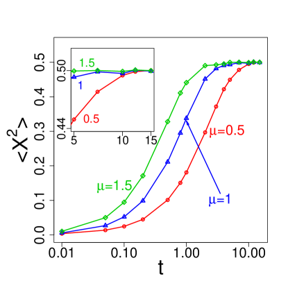
Figure 1: Gaussian target: Time evolution of the pdf $\rho(x,t)$ second moment for 75 000 trajectories. Inset visualize the oscillations smoothing in the asymptotic regime for $10\leq t\leq 15$; figures near curves correspond to $\mu$ values.

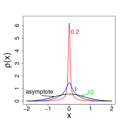
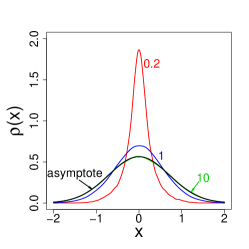
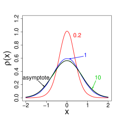
Figure 2: Gaussian target: Time evolution of $\rho(x,t)$ inferred from 75 000 trajectories: $\mu=0.5$ (left panel), $\mu=1$ (middle panel) and $\mu=1.5$ (right panel). All trajectories originate from $x=0$, i.e. refer to the $\delta(x)$-type initial probability distribution.

The results of our numerical simulations are reported in Figs. 1 and 2. We note, that in Fig. 1 the second moment oscillates near its equilibrium value $1/2$. A numerical convergence to $<X^{2}>=$$1/2$ is consistent with an analytic equilibrium value of the second moment of the chosen $\rho_{*}(x)$ 6. The rate of this convergence is higher for larger $\mu\in(0,2)$. Clearly, for small $\mu$ the big jumps are frequent which enlarges the inferred time intervals $\Delta t$ in the Gillespie’s algorithm. Thus, the relaxation to equilibrium is slow. It gets faster for larger $\mu$, when big jumps are rare and time intervals $\Delta t$ are generically very small.

Fig. 2 displays a probability density evolution, inferred from the ensemble statistics of $75000$ trajectories. All of them have started form the same point $x=0$. Although the data fidelity grows with the number of contributing paths, we have not found significant qualitative differences to justify a presentation of data for 100 000, 200 000, 250 000 and more trajectories. The relaxation time rate dependence on $\mu$ is clearly visible as well. It suffices to analyze differences between three curves for $t=0.2$ and/or $t=1$. We observe a conspicuous lowering of their maxima with the growth of $\mu$ (take care of different scales on the vertical axes on Fig.2 panels). The simulated pdfs at $t=10$ are practically indistinguishable from an exact analytical asymptotic pdf 6. The convergence of $\rho(x,t)$ towards $\rho_{*}(x)$ appears to be relatively fast irrespective of the chosen $\mu$-driver.

Although our reasoning is definitely path-wise and all data have been extracted from simulated trajectory ensembles, our focus was on the inferred dynamics of $\rho(x,t)$. We do not reproduce figures visualizing generic sample paths. However, we indicate their (paths) distinctive qualitative typicalities, if one would compare e.g. motion scenarios corresponding to stability indices $\mu=1/2$, $\mu=1$ and $\mu=3/2$, The structural impact (probability of occurrence) of larger against smaller jumps, even on the visual level, conforms with standard simulations of Lévy stable sample paths (with no forces or potentials involved), c.f. janicki .

III.2 Logarithmic confinement

III.2.1 Quadratic Cauchy target

Let us consider a long-tailed asymptotic pdf which is a special $\alpha=2$ case of the one-parameter $\alpha$-family of equilibrium (Boltzmann-type) states, associated with a logarithmic potential $\Phi(x)\equiv\alpha\ln(1+x^{2})$, $\alpha>1/2$, see gar ; gar0 ; gar1 ; gar2 :

$$\rho_{*}(x)=\frac{2}{\pi}\frac{1}{(1+x^{2})^{2}}.$$ (8)

The transition rate 2 $w_{\phi}(z+x|x)$ for any $\mu\in(0,2)$ takes the form

$$w_{\phi}(z+x|x)=\frac{C_{\mu}}{|z|^{1+\mu}}\frac{1+x^{2}}{1+(z+x)^{2}}.$$ (9)

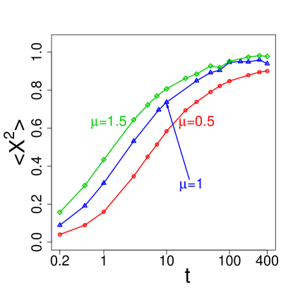
Figure 3: Quadratic Cauchy target: Time evolution of the pdf $\rho(x,t)$ second moment for 200 000 trajectories.

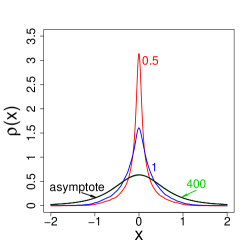
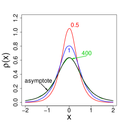
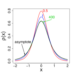
Figure 4: Quadratic Cauchy target: Time evolution of $\rho(x,t)$ inferred from $200000$ trajectories for $\mu=0.5$ (left panel), $\mu=1$ (middle panel) and $\mu=1.5$ (right panel). All trajectories are started from $x=0$. Note scale differences on vertical axes.

Simulation results for this case are displayed in Figs. 3 and 4. If we compare Fig. 3 with Fig. 1 we see the existence of small oscillations in the asymptotic regime about the value $1/2$. Those from Fig.1 were relatively small, while those on Fig. 3 are more noticeable. This is related to much slower decay of transition rates (9) (determined by slow-decaying asymptotic pdf (8)), as compared to those for Gaussian case (7).

The second moment of the present $\rho_{*}(x)$, (8), equals 1 and the convergence towards this value is clearly seen in Fig. 3. This convergence is much slower than in the Gaussian (harmonic confinement) case which is not a surprise: (7) and (9) indicate that the present rate of convergence should be logarithmically slower. Fig. 5, quite alike Fig. 2, convincingly demonstrates a convergence of $\rho(x,t)$ to the asymptotic $\rho_{*}(x)$. For definitely large times around $t=400$, $\rho(x,t)$ and $\rho_{*}(x)$ become practically indistinguishable. Similarly to the Gaussian case, the rate of convergence becomes larger with the growth of $\mu\in(0,2)$.

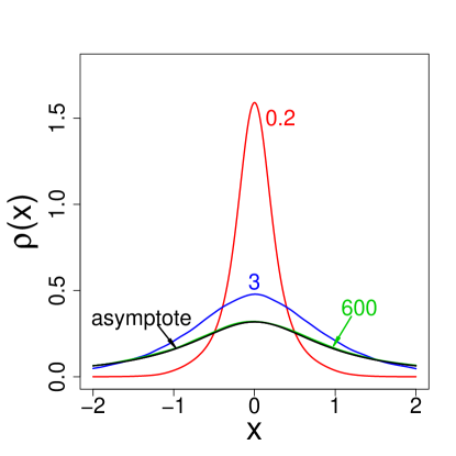
Figure 5: Cauchy target: Time evolution of pdf $\rho(x,t)$ for $\mu=1$ and $200000$ trajectories, starting from $x=0$.

III.2.2 Cauchy target

Now we consider an asymptotic pdf of the form :

$$\rho_{*}(x)=\frac{1}{\pi}\frac{1}{1+x^{2}}.$$ (10)

In this case, the transition rate from $x$ to $x+z$ reads

$$w_{\phi}(z+x|x)=\frac{C_{\mu}}{|z|^{1+\mu}}\sqrt{\frac{1+x^{2}}{1+(z+x)^{2}}}.$$ (11)

We consider Cauchy driver corresponding to $\mu=1$. In Fig. 5, we report the time evolution of the statistically inferred $\rho(x,t)$ for different time instants. An approach to the asymptotic pdf (10) is clearly seen, together with a convergence of a half-width to its asymptotic value 1. It can be shown that the same convergence pattern is valid for cumulative probability distribution which approaches the asymptotic function $F(x)=\frac{1}{2}+\frac{\arctan x}{\pi}$.

III.3 Locally periodic confinement

To set firm grounds for future research it is instructive to study our model for more complicated forms of confining potentials. In view of their physical relevance, it is appealing to address an issue of confining (trapping) environments with a periodic spatial structure. This problem may be relevant to the random motion of defects in doped semiconductors and to phenomena like hopping conductivity. Here, we encounter a major difficulty with integrability of the Boltzmann-type weighting function $\exp(-\Phi)$ as for periodic $\Phi$ the corresponding integral is divergent. Periodicity and integrability can here be reconciled by means of locally periodic potentials that take a definite confining form (harmonic or polynomial) for larger values of $x\in R$. Let us consider the following asymptotic pdf

$$\rho_{*}(x)=\left\{\begin{array}[]{ll}\frac{1}{C}e^{-\sin^{2}(2\pi x)},&\hbox{$|x|\leq 2$;}\\ \frac{1}{C}e^{-(x^{2}-4)},&\hbox{$|x|>2$,}\end{array}\right.$$ (12)

where $C=3.032818$ is a normalization constant. The transition rate from $x$ to $x+z$ reads

$$w_{\phi}(z+x|x)=\frac{C_{\mu}}{|z|^{1+\mu}}\exp{\left[(\phi(x)-\phi(x+z))/2\right]},$$ (13)

where the potential $\phi$ has the following locally confining form

$$\phi(x)=\left\{\begin{array}[]{ll}\sin^{2}(2\pi x),&\hbox{$|x|\leq 2$;}\\ (x^{2}-4),&\hbox{$|x|>2$.}\end{array}\right.$$ (14)

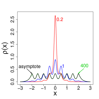
Figure 6: Time evolution of $\rho(x,t)$ inferred from $200000$ trajectories at $\mu=1$. The data for $100000$ and $300000$ trajectories (not displayed) do not show qualitative differences.

Time evolution of the inferred pdf $\rho(x,t)$ is reported in Fig. 6 for $\mu=1$. All sample trajectories were started form $x=0$ which corresponds to the $\delta(x)$-type initial distribution. The probability density spreads out with time in conformity with the trapping (confining) properties of the locally periodic enclosure (environment or ”potential landscape”). For large running times t=400 the trajectory statistics produces data that are indistinguishable from those for the asymptotic pdf. We have checked that beginning from about 100 000 trajectories, further accumulation of the trajectories number like e.g. 200 000 (displayed) and 300 000 (not displayed) for the data statistics is inessential. In such cases the curves are almost the same, we merely improve a fidelity of the statistics.

IV Conclusions.

If a random process does not admit the description in terms of a stochastic differential equation (e.g. Langevin modeling), its direct numerical simulation becomes impossible by means of existing popular algorithms. In the present paper, for the first time in the literature, we propose a working method to generate stochastic trajectories (sample paths) of a random jump-type process without resorting to any explicit (or numerical) solution of a stochastic differential equation.

To this end we have modified the Gillespie algorithm gillespie ; gillespie1 , normally devised for sample paths generation, if transition rates occur between a finite number of states of a system. The essence of our modification is that we take into account the continuum of possible transition rates, thereby changing the finite sums in the original Gillespie algorithm into integrals. The corresponding procedure for stochastic trajectories generation has been changed accordingly.

In other words, here we ”extract” the background sample paths of a jump process, whose pdf $\rho(x,t)$ is to obey the generalized Fokker-Planck dynamics 1, 2, . We emphasize once more here, that we have focused our attention on those background jump-type processes that cannot be modeled by any stochastic differential equation of the Langevin type. However, our ultimate result was a reconstruction of the pdf dynamics from the path-wise data. Thus, our modfication of the Gillespie’s algorithm serves two purposes: (i) getting access to path-wise data and (ii) reconstructing the pdf $\rho(x,t)$ dynamics, compatible with the master equation in question, without resorting to other methods of its solution

Although heavy-tailed Lévy stable drivers were involved in the present considerations, we have clearly confirmed that an enormous variety of stationary target distributions is dynamically accessible in each particular $\mu\in(0,2)$ case. That comprises not only a standard Gaussian pdf, discussed usually in relation to the Brownian motion like Wiener process. We can reach Cauchy pdf in terms of any $\mu\neq 1$ driver as well, provided a steering environment is properly devised. In turn, the Cauchy driver in a proper environment may lead to an asymptotic pdf with a finite number of moments, the Gaussian case included (gar ).

An example of the locally periodic environment has been considered as a toy model for more realistic physical systems. We mention possible generalizations of our method to the Brownian motor concept (see, e.g., Ref. browmot for recent review) to include a non-Gaussian jumping component. In those systems it is the properly tailored periodic ”potential landscape” which enforces a conversion of a homogenous stochastic process (Brownian motion for reference) into the directed motion of particles at nanometer scales. It is closely related to the problem of so-called sorting in periodic potentials presort . Other problems to be addresses concern ultracold atoms in optical lattices subject to random potentials coldopt , which are promising not only from purely scientific point of view, but also for many technological applications.

We note that the theoretical description of the above mentioned topics relies essentially on the Langevin-like equation input. Our approach offers prospects for generalizations, where systems with non-Langevin response to external potentials may come into consideration, along with more traditional ones. What we actually need to implement our version of Gillespie’s algorithm is the knowledge of jump transition rates of those random systems only.

Our preliminary work (in progress) shows that an extension of our algorithm to higher dimensions is operational. In particular, the planar case is worth further analysis, possibly with more realistic ”potential landscapes”. The direct numerical modeling in three-dimensional case can also be important, for instance, in the investigations of the dynamics of amorphous materials. Theoretical studies of their physical properties have a longer history, starting in the eighties and even earlier bin86 ; hoh . These materials may comprise conventional glasses (see, e.g., par ), so-called spin bin86 ; par and orientational (for example, dipole) glasses hoh as well as virtually any disordered solid like doped semiconductors. In these substances, the random motion of defects can be regarded as real jump-type process to be modeled numerically. Moreover, if defects have only rotational degrees of freedom (like spins or electric/elastic dipoles), their dynamics can be well represented by some effective jump-type process. Such representation can be complementary to existing Monte-Carlo modeling techniques which for disordered systems are very computer intensive. For instance, we hope to tackle the issue of interplay between exponential and long-time (logarithmic or stretched-exponential) relaxation in these substances. Also, the 3D modification of our algorithm can be used in the simulation of switching processes in disordered ferroelectrics my11 . Similar fictitious jump-type process can be assigned to the dynamics of inhomogeneous broadening of resonant lines sto . This broadening occurs in condensed matter and/or biological species, in a number of spectroscopic manifestations like the electron paramagnetic resonance, nuclear magnetic resonance, optical and neutron scattering methods. It arises due to random electric and magnetic fields, strains and other perturbations from defects in a substance containing the centers whose resonant transitions between energy levels are studied. Here also, the standard approaches cannot describe all the details of experiment and we hope that our algorithm can improve the situation.

Let us finally note that in the 3D problems admitting full spherical symmetry (like spin glasses with random exchange interactions), the problem becomes reducible to 1D case so that our algorithm might work in its present form.

Acknowledgement: P. G. would like to thank Professor I. M. Sokolov for focusing our attention on the Gillespie’s algorithm. All numerical simulations were completed by means of the facilities of the Platon - Science Services Platform of the Polish Pionier Network.

References

- (1) H. S. Wio, R.R. Deza, J.M. Lopez, An Introduction to Stochastic Processes and Nonequilibrium Statistical Physics, (World Scientific Publishing, Singapore, 2012).
- (2) V.A.Stephanovich, JETP Letters 65, 446 (1997).
- (3) H. Risken, The Fokker-Plack Equation, (Springer-Verlag, Berlin, 1989)
- (4) S. Jespersen, R. Metzler and H. C. Fogedby, Phys. Rev. E 59, 2736, (1999)
- (5) R. Metzler, J. Klafter, J. Phys. A:Math. Gen. 37, R161, (2004)
- (6) L. Chen and M. W. Deem, Phys. Rev. E 65, 011109, (2001)
- (7) D. Brockmann and I. M. Sokolov, Chemical Physics, 284, 409, (2002)
- (8) D. Brockmann and T. Geisel, Phys. Rev. Lett. 90, 170601, (2003)
- (9) V. V. Belik and D. Brockmann, New. J. Phys. 9, 54, (2007)
- (10) P. Garbaczewski and R. Olkiewicz, J. Math. Phys. 40, 1057, (1999)
- (11) P. Garbaczewski and R. Olkiewicz, J. Math. Phys. 41, 6843, (2000)
- (12) P. Garbaczewski and V. A. Stephanovich, Phys. Rev. E 80, 031113, (2009)
- (13) P. Garbaczewski and V. Stephanovich, Open Systems & Information Dynamics, 17, 287, (2010)
- (14) P. Garbaczewski and V. A. Stephanovich, Physica A 389, 4410, (2010)
- (15) P. Garbaczewski and V. Stephanovich, Phys. Rev. E 84, 011142 (2011)
- (16) P. Garbaczewski and V. A. Stephanovich, Acta Phys. Pol. B 43, 977, (2012)
- (17) J. Lőrinczi, F. Hiroshima and V. Betz, Feyman-Kac-Type Theorems and Gibbs Measures on Path Space, (Studies in Mathematics 34, Walter de Gruyter, Berlin, 2011)
- (18) R. Vilela Mendes, J. Math. Phys. 27,178, (1986)
- (19) S. Eleutério and R. Vilela Mendes, Phys. Rev. B 50, 5035, (1993).
- (20) I. Eliazar and J. Klafter, J. Stat. Phys. 111, 739, (2003)
- (21) V. V. Janovsky et al., Physica A 282, 13, (2000)
- (22) A. Dubkov and B. Spagnolo, Fluct. Noise Lett. 5, L267, (2005)
- (23) H. Touchette and E. G. D. Cohen, Phys. Rev. E 76, 020101, (2007)
- (24) T. Srokowski, Physica A 388, 1057, (2009)
- (25) T. D. Gillespie, J. Phys. Chemistry, 81 (25): 2340, (1977)
- (26) T. D. Gillespie, J. Comput. Physics, 22 (4): 403, (1976)
- (27) M. Matsumoto and T. Nishimura, ACM Trans. Model. Comput. Simul. 8, 3 (1998)
- (28) R. N. Mantegna and H. E. Stanley, Phys. Rev. Lett. 73, 2946, (1994)
- (29) I. M. Sokolov, private communication
- (30) C-code is available upon request
- (31) A. Janicki and A. Weron, Simulation and chaotic behavior of -stable stochastic processes, (M. Dekker, New York, 1994)
- (32) P. Hänggi, F. Marchesoni, Rev. Mod. Phys. 81, 387, (2009)
- (33) S. I. Denisov, T. V. Lyutyy et al, Phys. Rev. E 79, 051102, (2009)
- (34) H. Gimperlein, S. Wessel, J. Schmiedmayer, and L. Santos, Phys. Rev. Lett. 95, 170401, (2005)
- (35) K. Binder, A.P. Young, Rev. Mod. Phys. 58, 801 (1986).
- (36) U.T. Höchli, K. Knorr, A. Loidl, Adv. Phys. 39, 405 (1990).
- (37) G. Parisi, Field Theory, Disorder and Simulations, (World Scientific Publishing, Singapore, 1992).
- (38) D. Kedzierski, E.V. Kirichenko, V.A. Stephanovich, Phys. Lett. A 375, 685 (2011).
- (39) A.M. Stoneham, Rev. Mod. Phys. 41, 1 (1969).