Multi-sample Receivers Increase Information Rates
for Wiener Phase Noise Channels

Abstract

A waveform channel is considered where the transmitted signal is corrupted by Wiener phase noise and additive white Gaussian noise (AWGN). A discrete-time channel model is introduced that is based on a multi-sample receiver. Tight lower bounds on the information rates achieved by the multi-sample receiver are computed by means of numerical simulations. The results show that oversampling at the receiver is beneficial for both strong and weak phase noise at high signal-to-noise ratios. The results are compared with results obtained when using other discrete-time models.

I Introduction

Communication systems often suffer from phase noise that arises, e.g., due to the instability of RF oscillators in satellite [1] or microwave links [2]. In optical fiber communication, phase noise arises due to the instability of laser oscillators [3] or due to cross-phase modulation (XPM) in Wavelength-Division-Multiplexing (WDM) systems [4].

The nature of the phase noise depends on the application. A commonly studied discrete-time model is

$$Y_{k}={X}_{\text{symb},k}~{}e^{j\Theta_{k}}+Z_{k}$$ (1)

where $\{Y_{k}\}$ are the output symbols, $\{{X}_{\text{symb},k}\}$ are the input symbols, $\{\Theta_{k}\}$ is the phase noise process and $\{Z_{k}\}$ is additive white Gaussian noise (AWGN). For example, Katz and Shamai [5] studied the model (1) when $\{\Theta_{k}\}$ is independent and identically distributed (i.i.d.) according to $p_{\Theta}(\cdot)$, when $\Theta$ is uniformly distributed (called a noncoherent AWGN channel) and when $\Theta$ has a Tikhonov (or von Mises) distribution (called a partially-coherent AWGN channel). Tikhonov phase noise models the residual phase error in systems with phase-tracking devices, e.g., phase-locked loops (PLL) and ideal interleavers/deinterlevers.

Tight lower bounds on the capacities of memoryless noncoherent and partially coherent AWGN channels were computed by solving an optimization problem numerically in [5] and [6], respectively. Dauwels and Loeliger [7] proposed a particle filtering method to compute information rates for discrete-time continuous-state channels with memory and applied the method to (1) for Wiener phase noise and autoregressive–moving-average (ARMA) phase noise. Barletta, Magarini and Spalvieri [8] computed lower bounds on information rates for (1) with Wiener phase noise by using the auxiliary channel technique proposed in [9] and they computed upper bounds in [10]. They also developed a lower bound based on Kalman filtering in [11]. Barbieri and Colavolpe [1] computed lower bounds with an auxiliary channel slightly different from [8].

In this paper, we study a waveform channel corrupted by Wiener phase noise and AWGN:

$$r(t)=x(t)\ e^{j\theta(t)}+n(t),\text{ for }t\in\mathbb{R}$$ (2)

where $x(t)$ and $r(t)$ are the transmitted and received signals, respectively, while $n(t)$ and $\theta(t)$ are the additive and phase noise, respectively. A detailed description of the model is given in Sec. II. This model is reasonable, for example, for optical fiber communication with low to intermediate power and laser phase noise, see [3]. As pointed out in [12], the discrete-time model (1) does not fit the channel (2) because filtering a phase-varying signal with a constant amplitude gives rise to an output with a varying amplitude. The effect of filtering persists for phase impairments other than Wiener phase noise, e.g., for XPM in optical fiber [13]. We developed in [12] a discrete-time channel model based on a multi-sample receiver, i.e., a filter whose output is sampled multiple times per symbol.

In this paper, we use techniques based on [9] to compute tight lower bounds on the information rates for the multi-sample receiver introduced in [12]. The paper is organized as follows. The continuous-time model is described in Sec. II and the discrete-time model of the multi-sample receiver is described in Sec. III. We develop a method to compute lower bounds on the information rates of a multi-sample receiver in Sec. IV. In Sec. V, we report the results of numerical simulations and Sec. VI concludes the paper.

II Continuous-Time Model

We use the following notation: $j=\sqrt{-1}$ , ^∗ denotes the complex conjugate, $\delta_{D}$ is the Dirac delta function, $\lceil\cdot\rceil$ is the ceiling operator. We use $X^{k}$ to denote $(X_{1},X_{2},\ldots,X_{k})$. Suppose the transmit-waveform is $x(t)$ and the receiver observes

$$r(t)=x(t)\ e^{j\theta(t)}+n(t)$$ (3)

where $n(t)$ is a realization of a white circularly-symmetric complex Gaussian process $N(t)$ with

$$\mathbb{E}\left[N(t)\right]=0$$

$$\mathbb{E}\left[N(t_{1})N^{*}(t_{2})\right]=\sigma^{2}_{N}~{}\delta_{D}(t_{2}-t_{1}).$$ (4)

The phase $\theta(t)$ is a realization of a Wiener process $\Theta(t)$:

$$\Theta(t)=\Theta(0)+\int_{0}^{t}W(\tau)d\tau$$ (5)

where $\Theta(0)$ is uniform on $[-\pi,\pi)$ and $W(t)$ is a real Gaussian process with

$$\mathbb{E}\left[W(t)\right]=0$$

$$\mathbb{E}\left[W(t_{1})W(t_{2})\right]=2\pi\beta~{}\delta_{D}(t_{2}-t_{1}).$$ (6)

The processes $N(t)$ and $\Theta(t)$ are independent of each other and independent of the input. $N_{0}=2\sigma^{2}_{N}$ is the single-sided power spectral density of the additive noise. We define $U(t)\equiv\exp(j\Theta(t))$. The autocorrelation function of $U(t)$ is

$$R_{U}(t_{1},t_{2})=\mathbb{E}\left[U(t_{1})U^{*}(t_{2})\right]=\exp\left(-\pi\beta|t_{2}-t_{1}|\right)$$ (7)

and the power spectral density of $U(t)$ is

$$S_{U}(f)=\int_{-\infty}^{\infty}R_{U}(t,t+\tau)\ e^{-j2\pi f\tau}d\tau=\frac{\beta/2}{(\beta/2)^{2}+f^{2}}$$ (8)

The spectrum is said to have a Lorentzian shape. It is easy to show that $\beta=f_{\text{FWHM}}=2f_{\text{HWHM}}$ where $f_{\text{FWHM}}$ is the full-width at half-maximum and $f_{\text{HWHM}}$ is the half-width at half-maximum. Let $T$ be the transmission interval, then the transmitted waveforms must satisfy the power constraint

$$\mathbb{E}\left[\frac{1}{T}\int_{0}^{T}|X(t)|^{2}dt\right]\leq\mathcal{P}$$ (9)

where $X(t)$ is a random process whose realization is $x(t)$.

III Discrete-Time Model

Let $({x}_{\text{symb},1},{x}_{\text{symb},1},\ldots,{x}_{\text{symb},{n_{\text{symb}}}})$ be the codeword sent by the transmitter. Suppose the transmitter uses a unit-energy pulse $g(t)$ whose time support is $[0,T_{\text{symb}}]$ where $T_{\text{symb}}$ is the symbol interval. The waveform sent by the transmitter is

$$x(t)=\sum_{m=1}^{{n_{\text{symb}}}}{x}_{\text{symb},m}\ g(t-(m-1)T_{\text{symb}}).$$ (10)

Let $L$ be the number of samples per symbol ($L\geq 1$) and define the sample interval as

$$\Delta=\frac{T_{\text{symb}}}{L}.$$ (11)

The received waveform $r(t)$ is filtered using an integrator over a sample interval to give the output signal

$$y(t) =\int_{t-\Delta}^{t}r(\tau)\ d\tau.$$ (12)

The signal $y(t)$ is a realization of $Y(t)$ that is sampled at $t=k\Delta$, $k=1,\ldots,{n}={n_{\text{symb}}}L$, to yield the discrete-time model:

$$Y_{k}={X}_{\text{symb},\lceil k/L\rceil}\Delta\ e^{j\Theta_{k}}\ F_{k}+N_{k}$$ (13)

where $Y_{k}\equiv Y(k\Delta)$, $\Theta_{k}\equiv\Theta((k-1)\Delta)$,

$$F_{k}\equiv\frac{1}{\Delta}\int_{(k-1)\Delta}^{k\Delta}g\left(\tau-\left(\left\lceil\frac{k}{L}\right\rceil-1\right)T_{\text{symb}}\right)e^{j(\Theta(\tau)-\Theta_{k})}\ d\tau$$ (14)

and

$$N_{k} \equiv\int_{(k-1)\Delta}^{k\Delta}N(\tau)\ d\tau.$$ (15)

The process $\{N_{k}\}$ is an i.i.d. circularly-symmetric complex Gaussian process with mean $0$ and $\mathbb{E}[|N_{k}|^{2}]=\sigma^{2}_{N}\Delta$ while the process $\{\Theta_{k}\}$ is the discrete-time Wiener process:

$$\Theta_{k}=\Theta_{k-1}+W_{k}~{}\mod 2\pi$$ (16)

for $k=2,\ldots,n$, where $\Theta_{1}$ is uniform on $[-\pi,\pi)$ and $\{W_{k}\}$ is an i.i.d. real Gaussian process with mean $0$ and $\mathbb{E}[|W_{k}|^{2}]=2\pi\beta\Delta$, i.e., the probability distribution function (pdf) of $W_{k}$ is $p_{W_{k}}(w)=G(w;0,\sigma^{2}_{W})$ where

$$G(w;\mu,\sigma^{2})=\frac{1}{\sqrt{2\pi\sigma^{2}}}\exp\left(-\frac{(w-\mu)^{2}}{2\sigma^{2}}\right)$$ (17)

and $\sigma^{2}_{W}=2\pi\beta\Delta$. The random variable $(W_{k}\mod 2\pi)$ is a wrapped Gaussian and its pdf is $p_{W}(w;\sigma^{2}_{W})$ where

$$p_{W}(w;\sigma^{2})=\sum_{i=-\infty}^{\infty}G(w-2i\pi;0,\sigma^{2}).$$ (18)

Moreover, $\{F_{k}\}$ and $\{W_{k}\}$ are independent of $\{N_{k}\}$ but not independent of each other. Finally, equations (9) and (10) imply the power constraint

$$\frac{1}{{n_{\text{symb}}}}\sum_{m=1}^{{n_{\text{symb}}}}\mathbb{E}[|{X}_{\text{symb},m}|^{2}]\leq P=\mathcal{P}T_{\text{symb}}.$$ (19)

It is convenient to define $X_{k}$ as

$$X_{k}\equiv X(k\Delta)={X}_{\text{symb},\lceil k/L\rceil}~{}g\left((k\text{ mod }L)\Delta\right).$$ (20)

It follows that $I({X}_{\text{symb}}^{n_{\text{symb}}};Y^{n})=I(X^{n};Y^{n})$. We define the information rate

$$I(X;Y)=\lim_{{n_{\text{symb}}}\rightarrow\infty}\frac{1}{{n_{\text{symb}}}}I(X^{n};Y^{n}).$$ (21)

One difficuly in evaluating (21) is that the joint distribution of $\{F_{k}\}$ and $\{W_{k}\}$ is not available in closed form. Even the distribution of $F_{k}$ is not available in closed form (there is an approximation for small linewidth, see (16) in [3]). However, we can numerically compute tight lower bounds on $I(X;Y)$ by using the auxiliary-channel technique described next.

IV Lower Bound

The Auxiliary-Channel Lower Bound Theorem in [9, Sec. VI] states that for two random variables $X$ and $Y$, we have

$$I(X;Y) \geq\underline{I}(X;Y)=\mathbb{E}\left[\log\left(\frac{q_{Y|X}(Y|X)}{q_{Y}(Y)}\right)\right]$$ (22)

where $q_{Y|X}(\cdot|\cdot)$ is an arbitrary auxiliary channel and

$$q_{Y}(y)=\sum_{\tilde{x}}p_{X}(\tilde{x})q_{Y|X}(y|\tilde{x})$$ (23)

where $p_{X}$ is the true distribution of $X$. The distribution $q_{Y}(\cdot)$ is thus the output distribution obtained by connecting the true input source to the auxiliary channel. Using this theorem, we can compute a lower bound on $I(X;Y)$ by using the following algorithm [9]:

1. Sample a long sequence $(x^{n},y^{n})$ according to the true joint distribution of $X^{n}$ and $Y^{n}$.

2. Compute $q_{Y^{n}|X^{n}}(y^{n}|x^{n})$ and

   $$q_{Y^{n}}(y^{n})=\sum_{\tilde{x}^{n}}p_{X^{n}}(\tilde{x}^{n})q_{Y^{n}|X^{n}}(y^{n}|\tilde{x}^{n})$$ (24)

   where $p_{X^{n}}$ is the true distribution of $X^{n}$.

3. Estimate $\underline{I}(X;Y)$ using

   $$\underline{I}(X;Y)\approx\frac{1}{{n_{\text{symb}}}}\log\left(\frac{q_{Y^{n}|X^{n}}(y^{n}|x^{n})}{q_{Y^{n}}(y^{n})}\right)$$ (25)

Auxiliary Channel I

Consider the auxiliary channel

$$\Psi_{k}=X_{k}\Delta\ e^{j\Theta_{k}}+N_{k}$$ (26)

where $\{\Theta_{k}\}$ and $\{N_{k}\}$ are defined in Sec. III and $X_{k}$ is defined by (20). The channel $\Psi$ is the same as $Y$ in (13) except that $F_{k}$ is replaced with $g\left((k\mod L)\Delta\right)$. The channel is described by the conditional distribution $p_{\Psi^{n}|X^{n}}$

$$p_{\Psi^{n}|X^{n}}(y^{n}|x^{n}) =\int_{\theta^{n}}p_{\Theta^{n},\Psi^{n}|X^{n}}(\theta^{n},y^{n}|x^{n})\ d\theta^{n}$$ (27)

where

$$p_{\Theta^{n},\Psi^{n}|X^{n}}(\theta^{n},y^{n}|x^{n})$$

$$=\prod_{k=1}^{n}p_{\Theta_{k}|\Theta_{k-1}}(\theta_{k}|\theta_{k-1})\ p_{\Psi|X,\Theta}(y_{k}|x_{k},\theta_{k})$$ (28)

with

$$p_{\Theta_{k}|\Theta_{k-1}}(\theta|\tilde{\theta})=\left\{\begin{array}[]{ll}p_{W}(\theta-\tilde{\theta};\sigma^{2}_{W}),&k\geq 2\\ 1/(2\pi),&k=1\end{array}\right.$$ (31)

and

$$p_{\Psi|X,\Theta}(y|x,\theta)=\frac{1}{\pi\sigma^{2}_{N}\Delta}\exp\left(-\frac{\left|y-x~{}e^{j\theta}\right|^{2}}{\sigma^{2}_{N}\Delta}\right).$$ (32)

The channel $p_{\Psi^{n}|X^{n}}$ has continuous states $\theta^{n}$, which makes step 2 of the algorithm computationally infeasible.

Auxiliary Channel II

We use the following auxiliary channel for the numerical simulations:

$$\Upsilon_{k}=X_{k}\Delta\ e^{jS_{k}}+N_{k}$$ (33)

which has the conditional probability

$$p_{\Upsilon^{n}|X^{n}}(y^{n}|x^{n}) =\sum_{s^{n}\in\mathcal{S}^{n}}p_{S^{n},\Upsilon^{n}|X^{n}}(s^{n},y^{n}|x^{n})$$ (34)

where $\mathcal{S}$ is a finite set and

$$p_{S^{n},\Upsilon^{n}|X^{n}}(s^{n},y^{n}|x^{n})$$

$$=\prod_{k=1}^{n}p_{S_{k}|S_{k-1}}(s_{k}|s_{k-1})\ p_{\Psi|X,\Theta}(y_{k}|x_{k},s_{k})$$ (35)

where

$$p_{S_{k}|S_{k-1}}(s|\tilde{s})=\left\{\begin{array}[]{ll}Q(s|\tilde{s}),&k\geq 2\\ 1/|\mathcal{S}|,&k=1.\end{array}\right.$$ (38)

Next, we describe our choice of $\mathcal{S}$ and $Q(\cdot|\cdot)$. We partition $[-\pi,\pi)$ into $S$ intervals with equal lengths and pick the mid points of these intervals to be the elements of $\mathcal{S}$, i.e., we have

$$\mathcal{S}=\left\{\hat{s}_{i}:i=1,\ldots,S\right\}\text{ where }\hat{s}_{i}=i\frac{2\pi}{S}-\frac{\pi}{S}-\pi.$$ (39)

The state transition probability $Q(\cdot|\cdot)$ is chosen similar to [8] and [10]:

$$Q(s|\tilde{s})=\frac{2\pi}{S}{\int_{(\phi,\tilde{\phi})\in\mathcal{R}(s)\times\mathcal{R}(\tilde{s})}p_{W}(\phi-\tilde{\phi};\sigma^{2}_{W})\ d\phi d\tilde{\phi}}$$ (40)

where $\mathcal{R}(s)=[s-{\pi}/{S},s+{\pi}/{S})$, i.e., $\mathcal{R}(s)$ is the interval whose midpoint is $s$. The larger $S$ and $L$ are, the better the auxiliary channel (33) approximates the actual channel (13). We remark that even for small $S$ and $L$, the auxiliary channel gives a valid lower bound on $I(X;Y)$.

IV-A Computing The Conditional Probability

Suppose the input $X^{n}$ has the distribution $p_{X^{n}}$. A Bayesian network for $X^{n},S^{n},\Upsilon^{n}$ is shown in Fig. 1.

Figure 1: Bayesian network for ${X^{n},S^{n},\Upsilon^{n}}$ for $n=9$.

The probability $p_{\Upsilon^{n}|X^{n}}(y^{n}|x^{n})$ can be computed using

$$p_{\Upsilon^{n}|X^{n}}(y^{n}|x^{n})=\sum_{s\in\mathcal{S}}\rho_{n}(s)$$ (41)

where we recursively compute

$$\rho_{k}(s) \equiv p_{S_{k},\Upsilon^{k}|X^{n}}(s,y^{k}|x^{n})$$ (42)

$$\stackrel{{\scriptstyle(a)}}{{=}}\sum_{\tilde{s}\in\mathcal{S}}p_{S_{k-1},S_{k},\Upsilon^{k}|X^{n}}(\tilde{s},s,y^{k}|x^{n})$$

$$\stackrel{{\scriptstyle(b)}}{{=}}\sum_{\tilde{s}\in\mathcal{S}}\rho_{k-1}(\tilde{s})\ p_{S_{k},\Upsilon_{k}|S_{k-1},\Upsilon^{k-1},X^{n}}(s,y_{k}|\tilde{s},y^{k-1},x^{n})$$

$$=\sum_{\tilde{s}\in\mathcal{S}}\rho_{k-1}(\tilde{s})\ Q(s|\tilde{s})\ p_{\Psi|X,\Theta}(y_{k}|x_{k},s)$$ (43)

with the initial value $\rho_{0}(s)=1/|\mathcal{S}|$. Step $(a)$ is a marginalization, $(b)$ follows from Bayes’ rule and the definition of $\rho_{k}$ in (42), while (43) follows from the structure of Fig. 1. We remark that (43) is the same as with independent $X_{1},\ldots,X_{n}$, e.g., see equation (9) in [14, Sec. IV].

IV-B Computing The Marginal Probability

Define $\textbf{Y}_{m}\equiv(Y_{(m-1)L+1},Y_{(m-1)L+2},\ldots,Y_{(m-1)L+L})$ and $\textbf{X}_{m}\equiv(X_{(m-1)L+1},X_{(m-1)L+2},\ldots,X_{(m-1)L+L})$. Suppose the input symbols are i.i.d. and ${X}_{\text{symb},m}\in\mathcal{X}$ where $\mathcal{X}$ is a finite set. Therefore, $p_{X^{n}}$ has the form

$$p_{X^{n}}(x^{n}) =\prod_{m=1}^{{n_{\text{symb}}}}p_{\textbf{X}}(\textbf{x}_{m}).$$ (44)

A Bayesian network for $X^{n},S^{n},\Upsilon^{n}$ is shown in Fig. 2.

Figure 2: Bayesian network for ${X^{n},S^{n},\Upsilon^{n}}$ for $n=9$ and $L=3$.

The probability $p_{\Upsilon^{n}}(y^{n})$ can be computed using

$$p_{\Upsilon^{n}}(y^{n})=\sum_{s\in\mathcal{S}}\psi_{{n_{\text{symb}}}}(s)$$ (45)

where $\psi_{m}(s)\equiv p_{S_{mL},\textbf{Y}^{m}}(s,\textbf{y}^{m})$ which can be computed using the recursion:

$$\psi_{m}(s)$$ (46)

$$=\sum_{\tilde{\textbf{x}}\in\mathcal{X}_{L}}p_{\textbf{X}}(\tilde{\textbf{x}})\ \sum_{\tilde{s}\in\mathcal{S}}\psi_{m-1}(\tilde{s})\ p_{S_{mL},\textbf{Y}_{m}|S_{(m-1)L},\textbf{X}_{m}}(s,\textbf{y}_{m}|\tilde{s},\tilde{\textbf{x}})$$

with the initial value $\psi_{0}(s)=1/|\mathcal{S}|$. The set $\mathcal{X}_{L}$ is

$$\mathcal{X}_{L}=\{x\cdot(g(\Delta),g(2\Delta),\ldots,g(L\Delta)):x\in\mathcal{X}\}.$$ (47)

We remark that $|\mathcal{X}_{L}|=|\mathcal{X}|$ and not $|\mathcal{X}|^{L}$. Next, we define

$$\chi_{m,L}(s,\tilde{s},\tilde{\textbf{x}})\equiv p_{S_{mL},\textbf{Y}_{m}|S_{(m-1)L},\textbf{X}_{m}}(s,\textbf{y}_{m}|\tilde{s},\tilde{\textbf{x}})$$ (48)

for $s,\tilde{s}\in\mathcal{S}$ and $\tilde{\textbf{x}}\in\mathcal{X}_{L}$. Computing $\chi_{m,L}(s,\tilde{s},\tilde{\textbf{x}})$ is similar to computing $\rho_{n}$ (see (43)). Intuitively, this is because a block of $L$ samples in Fig. 2 has a structure similar to Fig. 1. More precisely, $\chi_{m,L}(s,\tilde{s},\tilde{\textbf{x}})$ can be computed recursively by using

$$\chi_{m,\ell}(s,\tilde{s},\tilde{\textbf{x}})$$ (49)

$$=\sum_{\varsigma\in\mathcal{S}}\chi_{m,\ell-1}(\varsigma,\tilde{s},\tilde{\textbf{x}})\ Q\left(s|\varsigma\right)\ p_{\Psi|X,\Theta}\left(y_{(m-1)L+\ell}|\tilde{x}_{\ell},s\right)$$

with the initial value

$$\chi_{m,0}(s,\tilde{s},\tilde{\textbf{x}})=\left\{\begin{array}[]{ll}1,&s=\tilde{s}\\ 0,&\text{otherwise}.\end{array}\right.$$ (52)

Therefore, computing $p_{\Upsilon^{n}}(y^{n})$ involves two levels of recursion: 1) recursion over the symbols as described by (46) and 2) recursion over the samples within a symbol as described by (49).

V Numerical Simulations

We use two pulses with a symbol-interval time support:

• A unit-energy square pulse

  $$g_{1}(t)=\frac{1}{\sqrt{T_{\text{symb}}}}\text{rect}\left(\frac{t}{T_{\text{symb}}}\right)$$ (53)

  where

  $$\text{rect}(t)\equiv\left\{\begin{array}[]{ll}1,&|t|\leq 1/2,\\ 0,&\text{otherwise}.\end{array}\right.$$ (56)

• A unit-energy cosine-squared pulse

  $$g_{2}(t)=\frac{1}{\sqrt{T_{\text{symb}}/2}}\cos^{2}\left(\frac{\pi t}{T_{\text{symb}}}\right)\text{rect}\left(\frac{t}{T_{\text{symb}}}\right).$$ (57)

The first step of the algorithm is to sample a long sequence according to the true joint distribution of $X^{n}$ and $Y^{n}$. To generate samples according to the original channel (13), we must accurately represent digitally the continuous-time waveform (3). We use a simulation oversampling rate $L_{\text{sim}}$ = 1024 samples/symbol. After the filter (12), the receiver has $L$ samples/symbol distributed according to (13). Next, to choose a proper sequence length, we follow the approach suggested in [9]: for a candidate length, run the algorithm about 10 times (each with a new random seed) and check whether all estimates of the information rate agree up to the desired accuracy. We used ${n_{\text{symb}}}=10^{4}$ unless otherwise stated. We define the signal-to-noise ratio as $\textsf{SNR}\equiv{P}/{\sigma^{2}_{N}T_{\text{symb}}}={\mathcal{P}}/{\sigma^{2}_{N}}$.

For efficient implementation of (43), $p_{\Psi|X,\Theta}(\cdot|\cdot,\cdot)$ can be factored out of the summation to yield:

$$\rho_{k}(s) =p_{\Psi|X,\Theta}(y_{k}|x_{k},s)\overbrace{\sum_{\tilde{s}\in\mathcal{S}}\rho_{k-1}(\tilde{s})\ Q(s|\tilde{s})}^{\rho^{\prime}_{k}(s)}$$ (58)

Moreover, since $Q(\cdot|\cdot)$ can be represented by a circulant matrix due to symmetry, $\rho^{\prime}_{k}(\cdot)$ can be computed efficiently using the Fast Fourier Transform (FFT). Similarly, the computation of (49) can be done efficiently by factoring out $p_{\Psi|X,\Theta}(\cdot|\cdot,\cdot)$ and by using the FFT.

V-A Excessively Large Linewidth

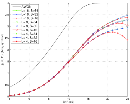
Figure 3: Lower bounds on rates for 16-QAM, square transmit-pulse and multi-sample receiver at $f_{\text{HWHM}}T_{\text{symb}}=0.125$.

Suppose $f_{\text{HWHM}}T_{\text{symb}}=0.125$ and the input symbols are independently and uniformly distributed (i.u.d.) 16-QAM. Fig. 3 shows an estimate of $\underline{I}(X;Y)$ for a square transmit-pulse, i.e., $g(t)=g_{1}(t-T_{\text{symb}}/2)$ and an $L$-sample receiver with $L=4,8,16$ and $S=16,32,64$. The curves with $S=64$ are indistinguishable from the curves with $S=32$ over the entire SNR range for all values of $L$, and hence $S=32$ is adequate up to 25 dB. Even $S=16$ is adequate up to 20 dB. The important trend in Fig. 3 is that higher oversampling rate $L$ is needed at high SNR to extract all the information from the received signal. For example, $L=4$ suffices up to SNR $\sim$ 10 dB, $L=8$ suffices up to SNR $\sim$ 15 dB but $L\geq 16$ is needed beyond that. It was pointed out in [9] that the lower bounds can be interpeted as the information rates achieved by mismatched decoding. For example, $\underline{I}(X;Y)$ for $L=8$ and $S\geq 32$ in Fig. 3 is essentially the information rate achieved by a multi-sample (8-sample) receiver that uses maximum-likelihood decoding for the simplified channel (26) when it is operated in the original channel (13).

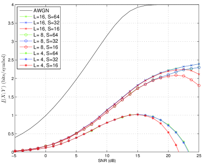
Figure 4: Lower bounds on rates for 16-QAM, cosine-squared transmit-pulse and multi-sample receiver at $f_{\text{HWHM}}T_{\text{symb}}=0.125$.

Fig. 4 shows an estimate of $\underline{I}(X;Y)$ for a cosine-squared transmit-pulse, i.e., $g(t)=g_{2}(t-T_{\text{symb}}/2)$ and an $L$-sample receiver at $L=4,8,16$ and $S=16,32,64$. We find that $S=32$ suffices up to $\sim$ 25 dB. We see in Fig. 4 the same trend in Fig. 3: higher $L$ is needed at higher SNR. Comparing Fig. 3 with Fig. 4 indicates that the square pulse is better than the cosine-squared pulse for the same oversampling rate $L$.

V-B Large Linewidth

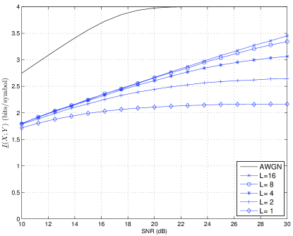
Figure 5: Lower bounds on rates for 16-PSK, square transmit-pulse and multi-sample receiver at $f_{\text{HWHM}}T_{\text{symb}}=0.0125$.

As the linewidth decreases, the benefit of oversampling at the receiver becomes apparant only at higher SNR. For example, for $f_{\text{HWHM}}T_{\text{symb}}=0.0125$ and i.u.d. 16-PSK input, Fig. 5 shows an estimate of $\underline{I}(X;Y)$ for a square transmit-pulse and an $L$-sample receiver at $L=1,2,4,8,16$ and $S=64$. We see that $L=4$ suffices up to SNR $\sim$ 19 dB, $L=8$ suffices up to SNR $\sim$ 24 dB and only beyond that $L\geq 16$ is necessary.

We conclude from Fig. 3–5 that the required $L$ depends on 1) the linewidth $f_{\text{FWHM}}$ of the phase noise; 2) the pulse $g(t)$; and 3) the SNR.

V-C Comparison With Other Models

We compare the discrete-time model of the multi-sample receiver with other discrete-time models. The simulation parameters for our model (GK) are ${n_{\text{symb}}}=10^{4}$, $L=16$ (with $L_{\text{sim}}=1024$) and $S=64$ for 16-QAM ($S=128$ was too computationally intensive) and $S=128$ for QPSK.

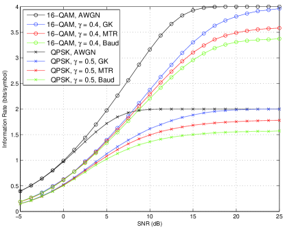
Figure 6: Comparison of information rates for different models.

In Fig. 6, we show curves for the Baud-rate model used in [1] and [7]–[11]. The model is (1) where the phase noise is a Wiener process whose noise increments have variance $\gamma^{2}$. We set $\gamma^{2}=2\pi\beta T_{\text{symb}}$. The simulation parameters for the Baud-rate model are ${n_{\text{symb}}}=10^{5}$ and $S=128$.

We also show curves for the Martalò-Tripodi-Raheli (MTR) model [14] in Fig. 6. For the sake of comparison, we adapt the model in [14] from a square-root raised-cosine pulse to a square pulse and write the “matched” filter output $\{V_{m}\}$ as

$$V_{m}=\sum_{\ell=1}^{L}\Psi_{(m-1)L+1}$$ (59)

where $m=1,\ldots,{n_{\text{symb}}}$ and $\Psi_{k}$ is defined in (26). The auxiliary channel is

$$Y_{m}={X}_{\text{symb},m}~{}e^{j\Theta_{m}}+Z_{m},\qquad m\geq 1$$ (60)

where the process $\{Z_{m}\}$ is an i.i.d. circularly-symmetric complex Gaussian process with mean $0$ and $\mathbb{E}[|Z_{m}|^{2}]=\sigma^{2}_{N}T_{\text{symb}}$ while the process $\{\Theta_{m}\}$ is a first-order Markov process (not a Wiener process) with a time-invariant transition probability, i.e., for $k\geq 2$ and all $\theta_{k},\theta_{k-1}\in[-\pi,\pi)$, we have $p_{\Theta_{k}|\Theta_{k-1}}(\theta_{k}|\theta_{k-1})=p_{\Theta_{2}|\Theta_{1}}(\theta_{k}|\theta_{k-1})$. Furthermore, the phase space is quantized to a finite number $S$ of states and the transition probabilities are estimated by means of simulation. The probabilities are then used to compute a lower bound on the information rate. The simulation parameters for the MTR model are ${n_{\text{symb}}}=10^{5}$, $L=16$ and $S=128$.

We see that the Baud-rate and MTR models saturate at a rate well below the rate achieved by the multi-sample receiver. Moreover, the multi-sample receiver achieves the full 4 bits/symbol and 2 bits/symbol of 16-QAM and QPSK, respectively, at high SNR.

VI Conclusion

We studied a waveform channel impaired by Wiener phase noise and AWGN by evaluating via numerical simulations tight lower bounds on the information rates achieved by a multi-sample receiver. We found that the required oversampling rate depends on the linewidth of the phase noise, the shape of the transmit-pulse and the signal-to-noise ratio. The results demonstrate that multi-sample receivers increase the information rate for both strong and weak phase noise at high SNR. We compared our results with the results obtained by using other discrete-time models.

References

- [1] A. Barbieri and G. Colavolpe, “On the information rate and repeat-accumulate code design for phase noise channels,” IEEE Trans. Commun., vol. 59, no. 12, pp. 3223 –3228, Dec. 2011.
- [2] G. Durisi, A. Tarable, and T. Koch, “On the multiplexing gain of MIMO microwave backhaul links affected by phase noise,” in IEEE Int. Conf. Commun. (ICC), Jun. 2013, to appear.
- [3] G. Foschini, L. Greenstein, and G. Vannucci, “Noncoherent detection of coherent lightwave signals corrupted by phase noise,” IEEE Trans. Commun., vol. 36, no. 3, pp. 306 –314, Mar. 1988.
- [4] R.-J. Essiambre, G. Kramer, P. J. Winzer, G. Foschini, and B. Goebel, “Capacity limits of optical fiber networks,” J. Lightwave Tech., vol. 28, no. 4, pp. 662 –701, Feb.15, 2010.
- [5] M. Katz and S. Shamai, “On the capacity-achieving distribution of the discrete-time noncoherent and partially coherent AWGN channels,” IEEE Trans. Inf. Theory, vol. 50, no. 10, pp. 2257 – 2270, Oct. 2004.
- [6] P. Hou, B. Belzer, and T. Fischer, “On the capacity of the partially coherent additive white Gaussian noise channel,” in IEEE Int. Symp. Inf. Theory, July 2003, pp. 372–372.
- [7] J. Dauwels and H.-A. Loeliger, “Computation of information rates by particle methods,” IEEE Trans. Inf. Theory, vol. 54, no. 1, pp. 406–409, Jan. 2008.
- [8] L. Barletta, M. Magarini, and A. Spalvieri, “Estimate of information rates of discrete-time first-order Markov phase noise channels,” IEEE Phot. Techn. Lett., vol. 23, no. 21, pp. 1582–1584, Nov. 2011.
- [9] D. Arnold, H.-A. Loeliger, P. Vontobel, A. Kavcic, and W. Zeng, “Simulation-based computation of information rates for channels with memory,” IEEE Trans. Inf. Theory, vol. 52, no. 8, pp. 3498 –3508, Aug. 2006.
- [10] L. Barletta, M. Magarini, and A. Spalvieri, “The information rate transferred through the discrete-time Wiener’s phase noise channel,” J. Lightwave Techn., vol. 30, no. 10, pp. 1480–1486, May 2012.
- [11] ——, “A new lower bound below the information rate of Wiener phase noise channel based on Kalman carrier recovery,” Opt. Express, vol. 20, no. 23, pp. 25 471–25 477, Nov. 2012. [Online]. Available: http://www.opticsexpress.org/abstract.cfm?URI=oe-20-23-25471
- [12] H. Ghozlan and G. Kramer, “On Wiener phase noise channels at high signal-to-noise ratio,” Submitted to IEEE Int. Symp. Inf. Theory, Jan. 2013, preprint available on http://arxiv.org/abs/1301.6923.
- [13] ——, “Interference focusing for simplified optical fiber models with dispersion,” in IEEE Int. Symp. Inf. Theory, Aug. 2011, pp. 376–379.
- [14] M. Martalò, C. Tripodi, and R. Raheli, “On the information rate of phase noise-limited communications,” in Inf. Theory and Applications Workshop, Feb. 2013.