$\mn@boldsymbol{\mu}$ Eridani from MOST and from the ground: an orbit, the SPB component’s fundamental parameters, and the SPB frequencies

Abstract

MOST time-series photometry of $\mu$ Eri, an SB1 eclipsing binary with a rapidly-rotating SPB primary, is reported and analyzed. The analysis yields a number of sinusoidal terms, mainly due to the intrinsic variation of the primary, and the eclipse light-curve. New radial-velocity observations are presented and used to compute parameters of a spectroscopic orbit. Frequency analysis of the radial-velocity residuals from the spectroscopic orbital solution fails to uncover periodic variations with amplitudes greater than 2 km s^-1. A Rossiter-McLaughlin anomaly is detected from observations covering ingress.

¿From archival photometric indices and the revised Hipparcos parallax we derive the primary’s effective temperature, surface gravity, bolometric correction, and the luminosity. An analysis of a high signal-to-noise spectrogram yields the effective temperature and surface gravity in good agreement with the photometric values. From the same spectrogram, we determine the abundance of He, C, N, O, Ne, Mg, Al, Si, P, S, Cl, and Fe.

The eclipse light-curve is solved by means of EBOP. For a range of mass of the primary, a value of mean density, very nearly independent of assumed mass, is computed from the parameters of the system. Contrary to a recent report, this value is approximately equal to the mean density obtained from the star’s effective temperature and luminosity.

Despite limited frequency resolution of the MOST data, we were able to recover the closely-spaced SPB frequency quadruplet discovered from the ground in 2002-2004. The other two SPB terms seen from the ground were also recovered. Moreover, our analysis of the MOST data adds 15 low-amplitude SPB terms with frequencies ranging from 0.109 d^-1 to 2.786 d^-1.

1 Introduction

The star $\mu$ Eri = HR 1520 = HD 30211 (B5 IV, $V={}$4.00 mag) was discovered to be a single-lined spectroscopic binary by Frost & Lee (1910) at Yerkes Observatory. An orbit was derived by Blaauw & van Albada (1963) from radial velocities measured on 19 spectrograms taken in November and December 1956 with the 82-inch McDonald Observatory telescope. The orbit was revised by Hill (1969) who supplemented the McDonald observations with the Yerkes radial-velocities (published by Frost, Barrett & Struve, 1926), Lick Observatory data of Campbell & Moore (1928) and Dominion Astrophysical Observatory (DAO) observations of Petrie (1958). Since these data span more than half a century, the value of the orbital period derived by Hill (1969) is given with six-digit precision, viz., $7.35886$ d.

The star was discovered to be variable in light by Handler et al. (2004) while being used as a comparison star in the 2002-2003 multi-site photometric campaign devoted to $\nu$ Eri. A frequency analysis of the campaign data revealed a dominant frequency of 0.616 d^-1. Prewhitening with this frequency resulted in an amplitude spectrum with a strong $1/f$ component indicating complex variation.

Using photometric indices and the Hipparcos parallax, Handler et al. (2004) determined the position of $\mu$ Eri in the HR diagram and compared it with evolutionary tracks. They found the star to lie close to a 6 M_☉ track, just before or shortly after the end of the main-sequence phase of evolution. Taking into account this result, the value of the dominant frequency, and the fact that the $u$ amplitude at this frequency is about a factor of two greater than the $v$ and $y$ amplitudes, Handler et al. (2004) concluded that $\mu$ Eri is probably an SPB star.

Handler et al. (2004) have also considered the possibility that the dominant variation is caused by rotational modulation. Assuming the dominant frequency to be equal to the frequency of rotation of the star and using a value of the radius computed from the effective temperature and luminosity, they obtained $\sim$190 km s^-1 for the equatorial velocity of rotation, $V_{\rm rot}$. This value and the published estimates of $V_{\rm rot}\sin i$, which range from 150 km s^-1 (Abt et al., 2002) to 190 km s^-1 (Bernacca & Perinotto, 1970), make rotational modulation a viable hypothesis. However, Handler et al. (2004) judged the hypothesis of rotational modulation to be less satisfactory than pulsations because it does not explain the complexity of the light variation.

The star was again used as the comparison star for $\nu$ Eri in the subsequent 2003-2004 multi-site photometric campaign (Jerzykiewicz et al., 2005, henceforth JHS05). The frequency of 0.616 d^-1 was confirmed and five further frequencies, ranging from 0.568 to 1.206 d^-1, were found. The multiperiodicity, the values of the frequencies and the decrease of the $uvy$ amplitudes with increasing wavelength implied high-radial-order $g$ modes, strengthening the conclusion of Handler et al. (2004) that $\mu$ Eri is an SPB variable.

An attempt at determining the angular degree and order, $\ell$ and $m$, of the six observed SPB terms was undertaken by Daszyńska-Daszkiewicz et al. (2008). Using a method of mode identification devised for SPB models in which the pulsation and rotation frequencies are comparable (Daszyńska-Daszkiewicz et al., 2007; Dziembowski et al., 2007), these authors obtained $\ell={}$1 and $m={}$0 for the dominant mode. In addition, they estimated the expected amplitude of this mode’s radial-velocity variation to be 5.9 km s^-1. For the remaining terms, there was some ambiguity in determining $\ell$ and $m$. Nevertheless, at least four terms detected in the star’s light variation could be attributed to unstable $g$ modes of low angular degree provided that the star was assumed to be still in the main-sequence phase of its evolution. For these four terms, the predicted radial-velocity amplitudes ranged from 0.6 km s^-1 to 13.1 km s^-1.

In addition to confirming the SPB classification, the analysis of the 2003-2004 campaign data showed $\mu$ Eri to be an eclipsing variable. As can be seen from figs. 3 and 5 of JHS05, the eclipse is a probably total transit, the secondary is fainter than the primary by several magnitudes, and the system is widely detached. The eclipse ephemeris, derived from the combined 2002-2003 and 2003-2004 campaign data, can be expressed as follows:

$${\rm Min.\ light}={\rm HJD}\,2452574.04\,(4)+7.3806\,(10)\,E.$$ (1)

Here, $E$ is the number of minima after the initial epoch given (which is that of the middle of the first eclipse, observed in 2002), and the numbers in parentheses are estimated standard deviations with the leading zeroes suppressed.

The photometric orbital period in equation (1) differs by more than 20 standard deviations from Hill’s (1969) period, mentioned in the first paragraph of this Introduction. Hill’s (1969) value is certainly less secure than the photometric value because it is based on a small number of observations, distributed unevenly over an interval of 53.2 years. In the periodogram of these observations, computed by Jerzykiewicz (2009), the three highest peaks in the period range of interest, all of very nearly the same height, occurred at 7.35889, 7.38116, and 7.38962 d. The first of these numbers corresponds to Hill’s (1969) value, while the second is equal to the photometric period to within half the standard deviation of the latter. Since both these numbers represent the radial-velocity data equally well, Jerzykiewicz (2009) concluded that the photometric period is the correct one.

Bruntt & Southworth (2008) observed $\mu$ Eri in February 2004 and August 2005 by means of the WIRE star tracker. After removing the SPB light-variation, they phased the observations with the orbital period of 7.381 d. Bruntt & Southworth (2008) suggest that the eclipse depth is variable.

The radial-velocity observations of Blaauw & van Albada (1963) and the photometric time-series data of Handler et al. (2004) and JHS05 were used by Jerzykiewicz (2009) to revise the spectroscopic orbital elements, solve the eclipse light-curve, and derive the primary’s mean density. The mean density turned out to be smaller than the value obtained from the position in the HR diagram determined by Handler et al. (2004), placing the star beyond the TAMS. This conflicts not only with the star’s photometric effective temperature, but also with the SPB classification because pulsational instability of $g$ modes disappears shortly after the minimum of $T_{\rm eff}$ in the main-sequence phase of evolution (Dziembowski et al., 1993). Improving the orbital elements of $\mu$ Eri and thus obtaining an accurate value of the mean density of the primary component in order to find out how severe these conflicts are was the motivation for undertaking the present work. In addition, we expected to verify the frequencies of the six SPB terms found by JHS05 and discover further frequencies, given that the photometric amplitudes are too small to be detected from the ground. Finally, we planned to look for the SPB radial-velocity variations predicted by Daszyńska-Daszkiewicz et al. (2008).

In the next section, we describe the MOST times-series photometry of $\mu$ Eri. In Section 3, we carry out a frequency analysis of these data and use the analysis results to remove the intrinsic component of the variation, thus bringing out the eclipse light-curve; in this section we also improve the eclipse ephemeris. In Section 4, we present new radial-velocity observations of $\mu$ Eri, some obtained contemporaneously with the MOST photometry, compute a spectroscopic orbit from them, and show that in the radial-velocity residuals from the orbital solution there are no periodic terms with an amplitude exceeding 2 km s^-1. In Section 5, we solve the eclipse light-curve by means of the computer program EBOP (Etzel, 1981). Section 6 deals with the Rossiter-McLaughlin effect. In Section 7, we determine the primary component’s fundamental parameters from (1) photometric indices and the revised Hipparcos parallax and (2) from high-resolution spectrograms; the spectrograms are also used to obtain the metal abundances by means of the method of spectrum synthesis. In Section 8, we derive the primary component’s mean density and discuss the star’s position in the HR diagram in relation to evolutionary tracks. Section 9 is devoted to assessing the SPB frequencies and amplitudes. The last section contains a summary of the results and suggestions for improvements. Short-period, small-amplitude variations found in the MOST observations of $\mu$ Eri are considered in the Appendix.

2 MOST time-series photometry

MOST (Walker et al., 2003) observed $\mu$ Eri in 2009, from November 4 to 16. The light curve is shown in Fig. 1. The two wide gaps seen in the figure divide the light curve into three parts: (1) from the first point at HJD 2455140.1633 to HJD 2455142.0219, (2) from HJD 2455142.5939 to HJD 2455146.1774, and (3) from HJD 2455146.5240 to the last point at HJD 2455152.1273. Part 1 throughout and part 2 from the beginning to HJD 2455145.1394 consist of 27 and 37 segments, respectively. The duration of most segments is equal to about 0.045 d, but there is one shorter segment in part 1 (0.0265 d), and two in part 2 (0.0098 d and 0.0356 d); the mean duration is equal to 0.0433 d. The mean duration of gaps between segments (not counting the gap between part 1 and part 2) amounts to 0.0259 d, and the mean interval between successive segments is equal to 101.4 min, the orbital period of the satellite. In part 2, from HJD 2455145.1554 to the end and in part 3 throughout there are less than one-hundred gaps, all shorter than 0.012 d. The shortest sampling interval and the number of data-points per unit time differ between segments and parts. In all segments of part 1 and the first 28 segments of part 2, the shortest sampling interval is equal to 0.0004 d and there are about 111 data-points per hour; in the remaining nine segments and the non-segmented portion of part 2 and in part 3, the shortest sampling interval is equal to 0.0007 d and there are about 55 data-points per hour.

Figure 1: The MOST light-curve of $\mu$ Eri. The vertical lines indicate estimated epochs of mid-eclipse.

The SPB variation time-scales are much longer than the duration of the data segments. It is therefore surprising that in many segments one can see short-term variations with ranges reaching 5 mmag. Short-term variations can be also seen in the non-segmented data. Further discussion of these variations we defer to the Appendix.

3 The eclipse

3.1 Frequency analysis of the out-of-eclipse data

In the light curve shown in Fig. 1, one can see the complex SPB variation and two successive eclipses. Unfortunately, in the first eclipse the ingress and the first half of the phase of totality are missing because of the first wide gap in the data. In addition, the eclipse is segmented (see Sect. 2), with the widest gap between segments (0.035 d) affecting the egress. We estimate the mid-eclipse epochs to be equal to HJD 2455142.60$\,\pm\,$0.03 d and HJD 2455149.98$\,\pm\,$0.02 d (see the vertical lines in Fig. 1). In order to obtain data suitable for analysing the SPB variation we modified the time series by omitting points falling within $\pm$0.03 orbital phase away from the mid-eclipse epochs. In the process, the number of data points was reduced from 15687 to 14765.

The power spectrum or periodogram of the modified data is shown in Fig. 2. Here and in what follows, by ‘power’ we mean $1-\sigma^{2}(f)/\sigma^{2}$, where $\sigma^{2}(f)$ is the variance of a least-squares fit of a sine curve of frequency $f$ to the data, and $\sigma^{2}$ is the variance of the same data.

Figure 2: The power spectrum of the out-of-eclipse data.

As expected, the power in the periodogram in Fig. 2 is concentrated in the frequency range $0<f\leq{}$1.4 d^-1, with a low-power alias around 14.2 d^-1, the orbital frequency of the satellite. This alias consists of the scaled-down pattern seen at low frequencies, shifted by 14.2 d^-1, and the mirror reflection about the $f={}$14.2 d^-1 axis of the scaled-down pattern. The periodogram in the frequency range 0${}<f\leq{}$1.4 d^-1 is displayed in the top panel of Fig. 3. The FWHM of the periodogram’s highest lobe, centered at $f_{1}={}$0.582 d^-1, is very nearly equal to $1/T={}$0.083 d^-1, where $T={}$12.0 d is the total time-span of the data. This shows that in our case the commonly used estimate of the frequency resolution, given by $1/T$, should be preferred over the more stringent value of $1.5/T$, advocated by Loumos & Deeming (1978).

Figure 3: The power spectrum of the out-of-eclipse data (top), after prewhitening with the frequency $f_{1}={}$0.582 d^-1 (middle), and after prewhitening with $f_{1}$ and $f_{2}={}$0.684 d^-1 (bottom).

In the middle panel of Fig. 3 there is shown the periodogram of the out-of-eclipse data prewhitened with the frequency $f_{1}$. The highest lobe, centered at $f_{2}={}$0.684 d^-1, has already appeared as a just-resolved feature in the periodogram of the original data in the top panel of the figure. Finally, the bottom panel shows the periodogram obtained after prewhitening the data with the two frequencies, $f_{1}$ and $f_{2}$. The power at low frequencies seen in this panel indicates a variation on a time scale longer than $T$. The isolated lobe at right is centered at 1.186 d^-1.

Fig. 4 shows the out-of-eclipse magnitudes prewhitened with $f_{1}$, $f_{2}$, and 1.186 d^-1. The long-term variation is clearly seen. A similar long-term variation was present in the MOST observations of $\delta$ Ceti. In the latter case it was shown by Jerzykiewicz (2007) to have been caused by inadequate compensation for background light in the MOST data reductions, so that the maximum of the variation occurred close to the phase of Full Moon, and the minimum, close to the phase of New Moon. The present case is similar. The upper line in Fig. 4 represents a segment of a sine-curve having a period equal to a synodic month and its maximum fixed at the phase of Full Moon, fitted to the data together with the three frequencies. Also shown in the figure is a linear trend, fitted to the data together with the same frequencies. The near coincidence of the two lines proves our point. However, the assumption that the maximum of the long-term variation occurs exactly at the phase of Full Moon may be unwarranted because it is not known how much of the variation is caused by direct illumination from the Moon (which is a function not only of the lunar phase, but also of the angular distance of the Moon from the spacecraft), and how much is due to increased earth-shine on moonlit nights. In addition, assuming the variation to be strictly sinusoidal may be an oversimplification. Unfortunately, the total time-span of the data is shorter than 0.4 of a synodic month, so that the significance of these two factors cannot be evaluated. For the same reason, including the synodic frequency in the analysis may affect the low SPB frequencies. Therefore, we decided to account for the long-term variation by subtracting a linear trend. Thus, the observational equations to be fitted by the method of least squares to the out-of-eclipse magnitudes, $m_{i}$, were assumed to have the following form:

$$m_{i}=A_{0}+Bt_{i}+\sum_{j=1}^{N}A_{j}\sin(2\pi f_{j}t_{i}+\Phi_{j}),$$ (2)

where the second term accounts for the trend and $t_{i}={}$HJD$-$2455146.

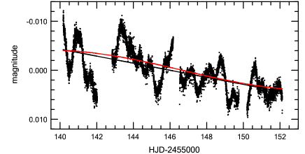
Figure 4: The out-of-eclipse magnitudes of $\mu$ Eri prewhitened with $f_{1}$, $f_{2}$, and 1.186 d^-1. The straight line (black) is a linear trend and the line running above it (red) is a segment of a sine-curve that has a period equal to a synodic month and maximum at the phase of Full Moon, fitted to the data together with the three frequencies. (A colour version of this figure is available in the online journal.)

The frequencies from $f_{3}$ to $f_{N}$ were then derived, one at a time, by determining the frequency of the highest peak in the periodogram computed after prewhitening with all frequencies already found and the trend. Adding the trend has affected the third frequency to be derived: it changed from 1.186 d^-1 to 1.193 d^-1. An attempt to refine the frequencies by means of the method of non-linear least squares was abandoned because (1) the “refined” frequencies differed grossly from their initial values, and (2) the solutions diverged for $N\geq{}$9. Parameters of equation (2) for $N={}$31 were computed by means of the linear least squares fit with frequencies read off the periodograms. The standard deviation of the fit was equal to 0.64 mmag, the first term, $A_{0}={}$4297.843$\,\pm\,$0.008 mmag, and the second term, $B={}$0.6253$\,\pm\,$0.0026 mmag d^-1. The frequencies, $f_{j}$, the amplitudes, $A_{j}$, and the phases, $\Phi_{j}$, are listed in Table 1 in order of decreasing amplitude. The signal-to-noise ratios, $S/N$, given in the last column, were computed using $A_{j}$ as $S$, and as $N$, the mean amplitude over a 1 d^-1 interval around $f_{j}$ in the amplitude spectrum of the data prewhitened with all 31 frequencies. The decrease of $S/N$ with $A_{j}$ is not monotonic because $N$ is a function of $f_{j}$. The amplitudes, and therefore the order of terms in Table 1, depend on the number of terms taken into account. This is why the third frequency derived from the periodograms is $f_{4}$ in the table. The frequencies which differ by less than $1/T$ from a frequency of larger amplitude are indicated with an asterisk. We included these frequencies because omitting them would defy our purpose of removing as much out-of-eclipse variation as possible from the light-curve. By the same token, we included terms with $S/N<{}$4.0 and those with $f_{j}>{}$15 d^-1 although the former are insignificant according to the popular criterion of Breger et al. (1993) while the latter are probably artefacts because they have frequencies that are either close to the whole multiples of the orbital period of the satellite or differ from the whole multiples by $\sim$1 d^-1. As shown in the Appendix, these frequencies are related to the short-term variations mentioned in Sect. 2.

Table 1: Frequencies, amplitudes and phases in the MOST out-of-eclipse magnitudes of $\mu$ Eri. The last column contains the signal-to-noise ratio.

$j$	$f_{j}$ [d-1]	$A_{j}$ [mmag]		$\Phi_{j}$ [rad]		S/N
1	0.582	6.618 $\pm$	0.011	1.550 $\pm$	0.002	254.5
2	0.684	4.567 $\pm$	0.011	2.904 $\pm$	0.002	175.7
3	0.387	2.843 $\pm$	0.013	4.789 $\pm$	0.004	109.3
4	1.193	2.523 $\pm$	0.009	1.322 $\pm$	0.004	84.1
5	0.297	1.812 $\pm$	0.012	2.849 $\pm$	0.008	69.7
6	0.232*	1.642 $\pm$	0.011	1.134 $\pm$	0.008	63.2
7	0.835	1.334 $\pm$	0.010	4.901 $\pm$	0.008	51.3
8	1.254*	1.200 $\pm$	0.008	0.781 $\pm$	0.007	40.0
9	0.109	1.177 $\pm$	0.011	5.305 $\pm$	0.008	45.3
10	1.035	1.058 $\pm$	0.009	5.327 $\pm$	0.009	37.8
11	1.115*	0.770 $\pm$	0.009	2.744 $\pm$	0.013	25.7
12	1.825	0.708 $\pm$	0.008	3.724 $\pm$	0.012	25.3
13	0.526*	0.556 $\pm$	0.010	1.864 $\pm$	0.021	21.4
14	2.423	0.446 $\pm$	0.008	2.985 $\pm$	0.018	17.2
15	1.620	0.333 $\pm$	0.009	1.915 $\pm$	0.025	11.1
16	0.754*	0.313 $\pm$	0.010	1.773 $\pm$	0.032	12.0
17	2.682	0.290 $\pm$	0.008	2.399 $\pm$	0.028	11.2
18	2.199	0.247 $\pm$	0.008	2.547 $\pm$	0.033	8.8
19	1.722	0.227 $\pm$	0.008	3.759 $\pm$	0.036	8.1
20	2.786	0.164 $\pm$	0.008	2.251 $\pm$	0.048	6.3
21	71.960	0.152 $\pm$	0.008	4.714 $\pm$	0.052	11.3
22	3.780	0.152 $\pm$	0.008	0.523 $\pm$	0.050	3.5
23	28.432	0.142 $\pm$	0.007	0.025 $\pm$	0.054	7.5
24	2.301	0.142 $\pm$	0.008	3.833 $\pm$	0.058	5.5
25	15.190	0.137 $\pm$	0.008	0.314 $\pm$	0.057	5.8
26	57.766	0.135 $\pm$	0.008	1.082 $\pm$	0.058	9.6
27	4.850	0.126 $\pm$	0.008	1.429 $\pm$	0.059	3.5
28	42.524	0.124 $\pm$	0.008	0.391 $\pm$	0.061	6.2
29	55.764	0.110 $\pm$	0.008	5.540 $\pm$	0.068	7.3
30	86.159	0.110 $\pm$	0.008	1.583 $\pm$	0.070	7.3
31	5.499	0.101 $\pm$	0.007	5.695 $\pm$	0.074	3.0

Figure 5: The residuals, $O-C$, from a least-squares fit of equation (2) with $N={}$31 to the out-of-eclipse data.

3.2 The eclipse light-curve and the corrected ephemeris

The residuals, $O-C$, where $O$ is the observed magnitude and $C$ is the magnitude computed from a least-squares fit of equation (2) with $N={}$31 to the out-of-eclipse data, are plotted in Fig. 5. From the residuals, the mid-eclipse epoch of the second eclipse could be derived much more accurately than was possible with the original data (see the first paragraph of Sect. 3.1). The result is HJD 2455149.973$\,\pm\,$0.002. Using this number and equation (1) we arrive at the following corrected ephemeris:

$${\rm Min.\ light}={\rm HJD}\,2455149.973\,(2)+7.38090\,(12)\,E,$$ (3)

where the notation is the same as before, except that the minima are now counted from the new, more accurate initial epoch. Note that the new value of the orbital period differs from the old value by about 0.3 of the standard deviation of the latter.

4 The spectroscopic orbit

4.1 The radial-velocity data

On 24 nights between 2 October 2009 and 8 February 2010, HL, MHa, and MHr obtained 105 spectrograms of $\mu$ Eri with the coudé echelle spectrograph at the 2-m Alfred Jensch telescope of the Thüringer Landessternwarte Tautenburg (TLS). The spectral resolving power was 63,000. The spectrograms were reduced using standard MIDAS packages. Reductions included bias and stray light subtraction, filtering of cosmic rays, flat fielding, optimum extraction of echelle orders, wavelength calibration using a ThAr lamp, correction for instrumental shifts using a large number of O₂ telluric lines, normalization to local continuum, and weighted merging of orders.

On eight nights, 4 to 14 November 2009, JM-Ż obtained 43 spectrograms of $\mu$ Eri with the 91-cm telescope and the fiber-fed echelle spectrograph FRESCO of the M.G. Fracastoro station of the Osservatorio Astrofisico di Catania (OAC). The spectral resolving power was 21,000. The spectrograms were reduced with IRAF.

Finally, on eight nights between 29 September 2009 and 22 January 2010, WD obtained 64 spectrograms of the star with the Poznań Spectroscopic Telescope (PST). The reductions were carried out by MF and KK by means of the Spectroscopy Reduction Package.

Radial velocities were determined from the spectrograms by EN by means of cross-correlation with a template spectrum in the logarithm of wavelength. A synthetic spectrum, computed assuming the photometric $T_{\rm eff}$ and $\log g$ (see Sect. 7.1), a microturbulence velocity of 4.0 km s^-1, $V_{\rm rot}\sin i={}$136 km s^-1, solar helium abundance, and the EN metal abundances from Table 6, served as the template. The wavelength intervals used in the cross-correlations included He I lines and lines of the elements listed in Table 6, had high signal-to-noise ratio (S/N), and were not affected by telluric lines. The S/N were determined with the IRAF task splot (function ”m”) from the continuum in the 5100 Å to 5800 Å range which contains only very faint lines. The S/N (per pixel) of the spectrograms ranged from 70 to 270 for TLS, from 60 to 110 for OAC, and from 40 to 120 for PST; the overall mean S/N values were 198$\,\pm\,$3, 93$\,\pm\,$2, and 78$\,\pm\,$2 for TLS, OAC, and PST, respectively.

Table 2: Nightly mean radial-velocities of $\mu$ Eri.

$\langle$HJD$\rangle$	$\langle$RV$\rangle$	$\langle$S/N$\rangle$	N	Obs
	[km s-1]
2455104.6491	28.35	87.7	3	PST
2455106.5913	$-$8.02	191.5	2	TLS
2455107.6194	13.82	179.4	2	TLS
2455113.6150	$-$7.24	210.0	1	TLS
2455135.5878	$-$4.29	200.5	2	TLS
2455136.6210	$-$4.76	210.0	1	TLS
2455140.5652	36.22	91.7	4	OAC
2455141.4761	30.84	110.5	4	PST
2455141.5661	30.12	226.0	2	TLS
2455142.5027	13.82	180.0	1	TLS
2455143.5048	$-$11.36	150.0	1	TLS
2455143.5660	$-$10.49	94.8	5	OAC
2455144.4553	4.17	110.0	1	OAC
2455146.5152	32.59	87.6	2	OAC
2455147.5578	36.65	216.0	2	TLS
2455147.5767	37.65	96.4	7	OAC
2455148.5484	35.66	92.5	7	OAC
2455149.5758	21.62	88.3	8	OAC
2455150.5478	$-$5.55	100.7	9	OAC
2455151.4388	$-$2.40	75.3	4	PST
2455155.4978	37.30	72.6	21	PST
2455155.5034	37.10	215.1	2	TLS
2455156.5190	30.64	67.3	8	PST
2455157.4154	9.53	69.0	3	PST
2455158.5251	$-$9.05	240.0	1	TLS
2455161.4549	37.23	87.7	14	PST
2455162.4466	32.40	180.0	1	TLS
2455163.4780	32.42	170.0	1	TLS
2455168.4333	31.12	190.0	1	TLS
2455170.4825	37.45	255.1	2	TLS
2455175.3956	29.30	230.0	1	TLS
2455192.4014	36.54	215.1	4	TLS
2455194.3866	2.94	230.0	1	TLS
2455199.3759	37.07	179.8	15	TLS
2455201.4046	21.68	225.1	4	TLS
2455202.3392	$-$12.10	191.4	34	TLS
2455219.3368	25.07	76.0	7	PST
2455228.3739	39.52	260.0	1	TLS
2455231.2637	3.63	270.0	1	TLS
2455236.2367	34.70	200.0	1	TLS

4.2 The spectroscopic elements

The number of spectrograms taken on a night ranged from one to 34. Using the individual radial-velocities of the preceding section for deriving a spectroscopic orbit would give excessive weight to the few nights with a large number of observations. To avoid this, we took weighted means of the individual velocities on nights with two or more observations using the S/N of the individual spectrograms as weights; the epochs of observations and S/N were likewise averaged. In Table 2 are given the single ($N={}$1) or the nightly weighted mean ($N\geq{}$2) epochs of observations, $\langle$HJD$\rangle$, the radial velocities, $\langle$RV$\rangle$, and the signal-to-noise ratios, $\langle$S/N$\rangle$. In the case of JD 2455201, the means were computed from the four points unaffected by the Rossiter-McLaughlin effect (see below, Sect. 6). Using the $\langle$HJD$\rangle$, $\langle$RV$\rangle$, and $\langle$S/N$\rangle$ from Table 2, we computed a spectroscopic orbit by means of the non-linear least squares method of Schlesinger (1908). We applied weights proportional to $\langle$S/N$\rangle$. The orbital period was assumed to be equal to the photometric period given in equation (3). An examination of the residuals from the solution revealed small systematic shifts between the TLS, OAC, and PST radial-velocities. Corrections to the OAC and PST radial-velocities which minimized the standard deviation of the solution turned out to be $-$0.09$\,\pm\,$0.73 km s^-1 and $-$0.15$\,\pm\,$0.71 km s^-1 for OAC and PST, respectively. The elements of the orbit, computed with these corrections taken into account, are listed in Table 3. Figure 6 shows the TLS radial-velocities and the corrected OAC and PST radial-velocities, plotted as a function of phase of the orbital period. The solid line is the radial-velocity curve computed from the elements listed in Table 3.

Table 3: Orbital elements of $\mu$ Eri computed from the radial-velocities of Table 2, with the systematic corrections added to the OAC and PST data (see text and Fig. 6).

$P_{\rm orb}$ (assumed)	7.38090 d
$T$	HJD 2455143.254 $\pm$ 0.067 d
$\omega$	160.5$\degr\,\pm$ 4.5$\degr$
$e$	0.344 $\pm$ 0.021
$\gamma$	20.58 $\pm$ 0.43 km s-1
$K_{1}$	24.24 $\pm$ 0.53 km s-1
$a_{1}\sin i$	3.320 $\pm$ 0.077 R☉
$f(M)$	0.00902 $\pm$ 0.00063 M☉

Figure 6: The TLS, OAC, and PST radial-velocities from Table 2, with the systematic corrections in the cases OAC and PST as indicated, plotted as a function of orbital phase. Also shown is the radial-velocity curve (line), computed from the spectroscopic elements of Table 3.

4.3 Looking for intrinsic radial-velocity variations

In an attempt to detect intrinsic radial-velocity variations, we examined the residuals from the orbital velocity curve of the 40 nightly mean radial-velocities used to derive it. A periodogram of these data, computed with weights proportional to $\langle$S/N$\rangle$ (see Table 2), showed the highest peak at $f={}$0.812 d^-1. Interestingly, this frequency is close to the JHS05 frequency ($f^{\prime}_{3}$ in their notation) for which Daszyńska-Daszkiewicz et al. (2008) predict the largest velocity amplitude (see the Introduction). However, the predicted amplitude of $f^{\prime}_{3}$ was equal to 13.1 km s^-1, while the amplitude of $f$ is equal to only 1.9$\,\pm\,$0.4 km s^-1. In addition, a periodogram of the residuals from the orbital velocity curve of the individual radial-velocity measurements (without those affected by the Rossiter-McLaughlin effect) showed the highest peak with the same amplitude but at a frequency of 0.626 d^-1, unrelated to $f$. We conclude that both these frequencies, $f$ and 0.626 d^-1, are spurious, and that in the radial-velocity residuals there are no periodic terms with an amplitude exceeding 2 km s^-1.

Unlike the PST and TLS observations, which fall mainly outside the interval covered by the MOST observations of $\mu$ Eri, all 43 OAC radial-velocities were obtained contemporaneously with the MOST photometry. Taking advantage of this, we have looked for a correlation between the OAC radial-velocity residuals and the trend-corrected MOST magnitudes. No correlation was found. Thus, the largest deviations from the orbital velocity curve, amounting to about $\pm\,$4.7 km s^-1 (see Fig. 6), are probably instrumental.

5 The eclipse light-curve solution

For computing the parameters of $\mu$ Eri from the eclipse light-curve we used Etzel’s (1981) computer program EBOP, which is based on the Nelson-Davis-Etzel model (Nelson & Davis, 1972; Popper & Etzel, 1981). The program is well suited for dealing with detached systems such as the present one. The spectroscopic parameters $\omega$ and $e$, needed to run the program, were taken from Table 3. The primary’s limb-darkening coefficient we computed by convolving the MOST KG filter transmission (Walker et al., 2003) with the monochromatic limb-darkening coefficients for $T_{{\rm eff}}={}$15 670 K and $\log g={}$3.5 (see Section 7.1) and [M/H] = 0 (Section 7.2). The monochromatic limb-darkening coefficients were interpolated in the tables of Walter Van Hamme. For the primary, the result was 0.308. For the secondary, assuming the effective temperature to scale as the square root of the radius and taking the ratio of the radii to be equal to 0.135 (see Table 4), we obtained $T_{\rm eff}={}$5 758 K. Using this value, we found the central surface brightness of the secondary in units of that of the primary (which EBOP uses as a fundamental parameter) to be equal to 0.018. Assuming further the solar value of 4.4 for $\log g$ and solar metallicity, and using the same tables of monochromatic limb-darkening coefficients as above, we computed the secondary’s limb-darkening coefficient to be equal to 0.628. The remaining parameters we set to their default EBOP values. The unknowns to be solved for were the orbital inclination, $i$, the ratio of the radii, $k=R_{\rm s}/R_{\rm p}$, and the radius of the primary, $r_{\rm p}=R_{\rm p}/a$, in units of the semi-major axis of the relative orbit, $a$. Initial values of the unknowns were derived by trial and error. Tests showed that the results were insensitive to the initial values.

Figure 7: Normal points computed in adjacent intervals of 0.0005 orbital phase using the $O-C$ residuals shown in Fig. 5. The solid line is the synthetic light-curve, computed with the parameters (4) of Table 4.

The results depend slightly on the light-curve data used. In Table 4 are shown the parameters obtained using (1) the $O-C$ residuals from a least-squares fit of equation (2) with $N={}$20 to the out-of-eclipse data, i.e., without terms $f_{j}>{}$15 d^-1, (2) normal points computed from the $O-C$ residuals in adjacent intervals of 0.0005 orbital phase; (3) and (4): the same as (1) and (2), respectively, but with $N={}$31. A synthetic light-curve computed with the parameters derived from data (4) (see Table 4) is compared with the data in Fig. 7; for orbital phases from $-$0.1 to 0.1, the synthetic light-curve is compared with the data in Fig. 8.

Table 4: The parameters of $\mu$ Eri derived by means of EBOP. Data (1) … (4) are explained in the text. SE is the EBOB standard error of one observation in mmags.

Data	SE	$i$	$k$	$r_{\rm p}$
(1)	0.71	82.06$\pm$0.07	0.13507$\pm$0.00011	0.2094$\pm$0.0005
(2)	0.48	82.11$\pm$0.12	0.13524$\pm$0.00021	0.2092$\pm$0.0008
(3)	0.64	82.42$\pm$0.07	0.13502$\pm$0.00010	0.2072$\pm$0.0004
(4)	0.41	82.44$\pm$0.11	0.13539$\pm$0.00018	0.2071$\pm$0.0007

Figure 8: The same as Fig. 7, but for a limited interval of orbital phase.

As can be seen from Fig. 8, the fit of the computed light-curve (line) to the observations (points) is not perfect at the bottom of the eclipse: before mid-eclipse the points fall below the lines, i.e., the system is fainter than computed, while after mid-eclipse the reverse is true. This looks like a signature of the rotational Doppler beaming, i.e., photometric Rossiter-McLaughlin effect (Groot, 2012; Shporer et al., 2012). However, from equation (3) of Shporer et al. (2012) it follows that in the present case the amplitude of the effect would be an order of magnitude smaller than the observed deviation.

The depth of the secondary eclipse predicted by the EBOP solution is 0.3 mmag, much smaller than the noise seen in Fig. 7. In the infrared, the depth of the secondary eclipse will be greater because the contribution of the primary to the total light of the system would decrease with increasing wavelength. The predicted MOST magnitude difference between components is 8.8 mag. Assuming that this number represents the magnitude difference in the $V$ band and using the standard $V-J$ and $V-K$ colour indices, one gets 2 mmag and 3 mmag as the depths of the secondary eclipse in J and K, respectively. Thus, detecting the secondary eclipse of $\mu$ Eri would be a task for a future infrared satellite.

6 The Rossiter-McLaughlin effect

Figure 9: Upper panel: individual radial-velocity measurements on JD 2455201 (open circles) plotted as a function of orbital phase. The short vertical lines indicate the epochs of first and second contact. Also shown are the radial-velocity curve, computed from the spectroscopic elements of Table 3 (solid line), and the radial-velocity curve plus the anomaly due to the Rossiter-McLaughlin effect, computed as explained in the text for $V_{\rm rot}\sin i={}$115 km s^-1 (dashed line). Lower panel: radial-velocity residuals (open circles) and the Rossiter-McLaughlin anomaly for $V_{\rm rot}\sin i={}$115 km s^-1, shifted upwards by 4.67 km s^-1 (dashed line), bracketed by those for $V_{\rm rot}\sin i={}$70 km s^-1 and $V_{\rm rot}\sin i={}$160 km s^-1 (the lower and upper dotted line, respectively).

On JD 2455201, there were 25 measurements, the first one at HJD 2455201.3958, and the last at HJD 2455201.5034. According to equation (3), the corresponding orbital phases (reckoned from the epoch of mid-eclipse) are equal to $-$0.033 and $-$0.018. Thus, the measurements start shortly before the ingress begins, and last to just after it ends. This is illustrated in the upper panel of Fig. 9, where the epochs of first and second contact, predicted by the eclipse solution (4) of Table 4, are indicated by short vertical lines. Also shown in the figure is a fragment of the orbital velocity curve, computed from the spectroscopic elements of Table 3 (solid line in the upper panel), and the deviations from this curve due to the Rossiter-McLaughlin effect (dashed line), computed assuming (1) the direction of rotation concordant with the direction of orbital motion, and (2) $V_{\rm rot}\sin i$ of the primary component equal to 115 km s^-1, a value that gave the best least-squares fit to the data. The lower panel of Fig. 9 shows the fit to the residuals, bracketed by the Rossiter-McLaughlin deviations for $V_{\rm rot}\sin i$ equal to 70 km s^-1 and 160 km s^-1 (the lower and upper dotted line, respectively). In computing the deviations we used formulae developed by Petrie (1938). These formulae assume the axis of rotation of the star to be perpendicular to the orbital plane, neglect limb darkening, and are valid for circular orbits. The last assumption was moderated to first order in the eccentricity by means of the prescription given by Russell (1912). Taking into account the effect of limb darkening would reduce the computed deviations (see Ohta et al. 2005), so that the best fitting $V_{\rm rot}\sin i$ would be greater by a factor of $\sim$1.5. We conclude that the increase of the radial-velocity residuals from about 4.5 km s^-1 to about 6 km s^-1, seen in the lower panel of Fig. 9, is consistent with $V_{\rm rot}\sin i$ of about 170$\,\pm\,$45 km s^-1, but we postpone a more detailed discussion of the Rossiter-McLaughlin effect in $\mu$ Eri until more accurate data become available. Note, however, that although the value of $V_{\rm rot}\sin i$ is not well constrained at this stage, the direction of rotation is determined beyond doubt.

On JD 2455201, the mean residual from the orbital solution amounted to 5.49$\,\pm\,$0.15 km s^-1. Subtracting the Rossiter-McLaughlin deviations (dashed line in Fig. 9) reduces this value to 4.67$\,\pm\,$0.10 km s^-1. The residual is probably instrumental (see Sect. 4.3).

7 Stellar parameters

7.1 From photometric indices and the revised Hipparcos parallax

The colour excess of $\mu$ Eri is small but not negligible. Using the star’s $B-V$ and $U-B$ colour indices from Mermilliod (1991) and Johnson’s (1966) standard two-colour relation for main-sequence stars, we get $E(B-V)={}$0.018$\,\pm\,$0.006 mag. From the Strömgren $uvby$ indices (Hauck & Mermilliod, 1998) and Crawford’s (1978) $(b-y)_{0}$ - $c_{0}$ relation, we have $E(b-y)={}$0.013$\,\pm\,$0.004 mag or $E(B-V)={}$0.018$\,\pm\,$0.005 mag. The dereddened colours and the $\beta$ index (Hauck & Mermilliod, 1998) then yield the effective temperature, $T_{\rm eff}$, the bolometric correction, BC, and the logarithmic surface gravity, $\log g$. The results are listed in Table 5, in columns three, four, and five, respectively. The BC values obtained using the calibrations of Balona (1994) and Flower (1996) were adjusted slightly (by 0.03 mag and 0.01 mag, respectively) in order to make them consistent with BC${}_{\sun}={}-$0.07 mag, the zero point adopted by Code et al. (1976). As can be seen from Table 5, Flower’s (1996) $T_{\rm eff}$ and BC are much lower than the other ones. The former values were obtained by interpolation from this author’s table 3. Using the polynomial fits provided by Flower (1996) and corrected by Torres (2010) results in $T_{\rm eff}$ and BC virtually identical with those given in Table 5. Omitting Flower’s (1996) values, we get 15 670 K and $-$1.40 mag for the mean $T_{\rm eff}$ and BC, respectively. Our value of $T_{\rm eff}$ is identical to those derived by Handler et al. (2004) and Daszyńska-Daszkiewicz et al. (2008) from Geneva photometry. However, while Handler et al. (2004) estimated the standard deviation of their value to be equal to 100 K, we believe that the standard deviation of $T_{\rm eff}$ cannot be smaller than the uncertainty of temperature calibrations, i.e., about 3 percent (Napiwotzki et al., 1993; Jerzykiewicz, 1994) or 470 K for the $T_{\rm eff}$ in question. Daszyńska-Daszkiewicz et al. (2008) give a somewhat more optimistic value of 365 K.

Taking into account the uncertainty of calibrations, we estimate the standard deviation of the bolometric correction to be equal to 0.08 mag. Finally, the mean value of $\log g$ is equal to 3.5 dex (see Table 5), with an estimated standard deviation of 0.15 dex.

Table 5: Fundamental parameters of $\mu$ Eri obtained from the photometric indices listed in column one, using the calibration referenced in column two.

Data	Calibration	$T_{\rm eff}$	BC	$\log g$
$(B-V)_{0}$	Code et al. (1976)	15 700	$-$1.47	–
$(B-V)_{0}$	Flower (1996)	14 610	$-$1.17	–
$c_{0}$	Davis & Shobbrook (1977)	15 670	$-$1.46	–
$c_{0}$, $\beta$	UVBYBETA	15740	–	3.44
$c_{0}$, $\beta$	Balona (1994)	15 580	$-$1.28	3.52

¿From the revised Hipparcos parallax (van Leeuwen, 2007), the $V$ magnitude from Mermilliod (1991), $E(B-V)$ from the first paragraph of this section, and assuming $R_{V}={}$3.1, we get $M_{V}={}-$2.06$\,\pm\,$0.07 mag, $M_{\rm bol}={}-$3.46$\,\pm\,$0.10 mag, and $\log L/{\rm L}_{\sun}={}$3.280$\,\pm\,$0.040. The standard deviations of $M_{\rm bol}$ and $\log L/$L_☉ are determined by the standard deviation of BC and the standard deviation of $M_{V}$ (in that order). In computing $\log L/$L_☉, we assumed M${}_{{\rm bol}{\sun}}={}$4.74 mag, a value consistent with BC${}_{\sun}=-{}$0.07 mag we adopted and $V_{\sun}={}-$26.76 mag (Torres, 2010).

7.2 From TLS spectra

A Fourier-transform based program KOREL (Hadrava, 2006a, b) was used to decompose the stellar spectrum and the telluric contributions with the orbital elements obtained in Section 4.2 adopted as starting values and the orbital period fixed at the photometric value. The result was a high-S/N spectrum of $\mu$ Eri, free of telluric contributions, representing a mean spectrum, averaged over all RV-shifted spectra of the TLS time-series. The analysis of this mean spectrum was carried out independently by HL and EN. HL used the program SynthV (Tsymbal, 1996) to compute a grid of synthetic spectra from LTE model atmospheres calculated with the program LLmodels (Shulyak et al., 2004). For a detailed description of the method see Lehmann et al. (2011). For the analysis, the full wavelength range 4720 Å to 7300 Å was used. The atomic line parameters were adopted from the Vienna Atomic Line Database (VALD). HL has derived the following parameters: $T_{\rm eff}={}$ 15 590$\,\pm\,$120 K, $\log g={}$3.55$\,\pm\,$0.04, the microturbulence velocity, $\xi={}$0.0$\,\pm\,$0.4 km s^-1, and $V_{\rm rot}\sin i={}$130$\,\pm\,$3 km s^-1. For the He abundance, HL has obtained 1.3$\,\pm\,$0.1 times the solar value. The errors are 1$\sigma$ errors from $\chi^{2}$ statistics as described in Lehmann et al. (2011). They represent a measure of the quality of the fit but do not account for imperfections of the model. Small corrections to the local continua of the observed spectra have been applied by comparing them to the synthetic spectra in the process of parameter determination. Possible correlations between the parameters are included by deriving the optimum values and their errors from the multidimensional surface in $\chi^{2}$ of the correlated parameters. A careful check for ambiguities between the parameters was performed. Besides the well-known correlation between $T_{\rm eff}$ and [M/H], we observe in the given temperature range a slight degeneracy between $T_{\rm eff}$ and $\log g$ and a strong correlation between $\log g$ and the He content. For the latter, we derive d $\log g/{\rm d\,He}={}-$0.15 from our LLmodel atmospheres, where He is the He abundance in units of the solar value. An enhanced He abundance generates additional pressure (Auer et al., 1966; Fossati et al., 2009), changing in our case $\log g$ from 3.36 for solar He abundance to 3.55 for 1.3 times solar abundance. The effect on $T_{\rm eff}$ is marginal, as also found by Fossati et al. (2009). We determine d $T_{\rm eff}{\rm/d\,He}={}$22 K. No degeneracy between any of the other parameters was found. A test of the influence of the abundances of different chemical elements showed that only a modification of the He, Ne, Si, S, and Fe abundances had a significant effect on the quality of the fit. Except for Ne, the metal abundances turned out to be very nearly solar. The numbers are given in the second column of Table 6; the standard deviations were estimated from $\chi^{2}$ statistics as described before.

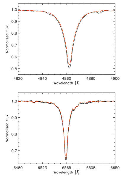
Figure 10: Upper panel: the observed mean profile of the H$\beta$ line (black, solid) and the synthetic profile, computed for $T_{\rm eff}={}$15 670 K, $\log g={}$ 3.5 dex, $\xi=4.0$ km s^-1, and $V_{\rm rot}\sin i={}$136 km s^-1 (red, dashed). Lower panel: the same for the H$\alpha$ line. (A colour version of this figure is available in the online journal.)

EN used the same mean spectrum as HL did, a grid of line-blanketed LTE model atmospheres computed with the ATLAS9 code (Kurucz, 1993a) and synthetic spectra computed with the SYNTHE code (Kurucz, 1993b). The stellar line identification in the entire observed spectral range was done using the line list of Castelli & Hubrig (2004). To begin with, the photometric $T_{\rm eff}$ and $\log g$ (see Sect. 7.1) were verified by comparing the observed profiles of the H$\beta$ and H$\alpha$ lines with the synthetic profiles, computed for $T_{\rm eff}$ from 15 000 K to 16 000 K with a step of 50 K, and $\log g$ from 3.0 dex to 4.0 dex with a step of 0.1 dex. The best match was obtained for 15500 K${}<T_{\rm eff}<{}$15700 K and 3.5 dex${}<\log g<{}$ 3.6 dex, in excellent agreement with the photometric values and with HL. Then, parts of the spectrum suitable for the analysis were selected. Next, the elements which influence every chosen part were identified. Finally, assuming the photometric $T_{\rm eff}$ and $\log g$, $\xi=4.0$ km s^-1, and solar helium abundance, the values of $V_{\rm rot}\sin i$ and the abundances were determined by means of the spectrum synthesis method described in Niemczura et al. (2009). The rotational velocity was derived from every part of the spectrum, whereas the abundance of a given element was determined from all parts in which this element was identified. The final values of $V_{\rm rot}\sin i$, and of the abundances are average values obtained from all parts in which they were determined. The final value of $V_{\rm rot}\sin i$ is equal to 136$\,\pm\,$6 km s^-1. A comparison of the TLS mean profiles of the H$\beta$ and H$\alpha$ lines with the synthetic profiles, computed with the photometric $T_{\rm eff}$ and $\log g$, $\xi=4.0$ km s^-1, and $V_{\rm rot}\sin i={}$ 136 km s^-1, is presented in Fig. 10.

The abundances with their standard deviations are given in the third column of Table 6, and the number of parts of the spectrum from which they were derived, $n$, in column four. The solar abundances listed in the last column are quoted from Asplund et al. (2006). Both, HL and EN determined the abundances of Ne, Si, S and Fe. Except for Si, the agreement between the HL and EN abundances is within 1 $\sigma$. In the case of Si, HL’s $\log N$ is virtually identical with $\log N_{\sun}$. As can be seen from Table 6, the C, N and O abundances determined by EN are slightly smaller then solar, whereas Al (only one part of the spectrum used) and P are enhanced. The abundances of Mg, S, Cl, Fe and Ni obtained by EN are close to the solar values. On the other hand, Ne is overabundant by 0.71$\,\pm\,$0.11 dex according to EN, and by 0.56$\,\pm\,$0.15  dex according to HL. The Ne abundances of B-type stars were investigated by Cunha et al. (2006) and Morel & Butler (2008). In these papers a non-LTE approach was adopted; the Ne abundances turned out to be equal to 8.11$\,\pm\,$0.04 and 7.97$\,\pm\,$0.07 dex, respectively. In addition, Cunha et al. (2006) found that the difference between the LTE and non-LTE abundance derived from the Ne I 6402 Å line amounted to 0.56 dex. This result is close to the difference between the HL and EN LTE-determinations and the non-LTE values of Cunha et al. (2006) and Morel & Butler (2008).

Table 6: The elemental abundances of $\mu$ Eri derived by HL and EN; $n$ is explained in the text.

Element	$\log N$	$\log N$	$n$	$\log N_{\sun}$
	HL	EN
He	11.04$\pm$0.034	–	–	10.93
C	–	8.26$\pm$0.27	6	8.39
N	–	7.41$\pm$0.29	3	7.78
O	–	8.49$\pm$0.31	3	8.66
Ne	8.40$\pm$0.26	8.55$\pm$0.11	13	7.84
Mg	–	7.51	2	7.53
Al	–	6.77	1	6.37
Si	7.49$\pm$0.21	7.11$\pm$0.12	7	7.51
P	–	5.82$\pm$0.21	5	5.36
S	6.94$\pm$0.20	7.06$\pm$0.18	18	7.14
Cl	–	5.51	1	5.50
Fe	7.45$\pm$0.30	7.34$\pm$0.23	20	7.45
Ni	–	6.21$\pm$0.15	3	6.23

In addition to differences in methodology and software, an important difference between the HL and EN analyses is the value of the microturbulence velocity. While HL derived $\xi={}$0.0 km s^-1, EN assumed 4.0  km s^-1 following Lefever et al. (2010). The main consequence of this difference is the following: For a strong line, greater $\xi$ results in a greater equivalent width of the line in the synthetic spectrum, so that matching the synthetic and observed line-profiles requires a smaller abundance than would be the case for a smaller $\xi$. The determination of the Si abundance is dominated by the strong Si II doublet at 6347/6371 Å. This explains why EN obtained appreciably smaller abundance of Si than did HL (see Table 6). In the case of Fe, there was one strong line, viz., Fe I at 5057 Å, and dozens of fainter lines; consequently, the effect is smaller than for Si. The effect is absent in the case of Ne and S because no strong lines were used in the analysis.

8 Mean density and the HR diagram

Using the effective temperature and luminosity obtained in Sect. 7.1 and assuming a mass of 6.2$\,\pm\,$0.2 M_☉ (see below) we find the mean density of the primary component, $\langle\rho\rangle_{\rm ph}={}$0.0418$\,\pm\,$0.0057 g cm^-3, where the suffix “ph” is a reminder of the photometric provenance of this value. Surprisingly, the largest contribution to the large standard deviation does not come from the standard deviation of $T_{\rm eff}$, but from that of $L$: if the latter were omitted, the standard deviation of $\langle\rho\rangle_{\rm ph}$ would be reduced to 0.0033 g cm^-3; omitting the former yields a standard deviation of 0.0048 g cm^-3.

A value of the mean density independent of photometric calibrations can be derived in the present case because for a binary with the primary’s mass much larger than that of the secondary, the spectroscopic and photometric elements can be combined to derive a mass-radius relation

$$M_{\rm p}\sim R_{\rm p}^{3+x},$$ (4)

where $R_{\rm p}$ is the radius of the primary and $x$ is a small positive number, slowly varying with $M_{\rm p}$, the assumed mass of the primary (Pigulski & Jerzykiewicz, 1981). A consequence of this relation is that the mean density of the primary computed from the orbital solution, $\langle\rho\rangle_{\rm orb}$, is weakly dependent on $M_{\rm p}$. This fact has been used by Dziembowski & Jerzykiewicz (1996) to derive a mean density of the $\beta$ Cephei primary of 16 Lac (EN Lac), an SB1 and EA system rather similar to $\mu$ Eri. In the present case, the spectroscopic parameters $K_{1}$ and $e$ from Table 3 and the photometric parameters $r_{\rm p}$ and $i$ from line (3) or (4) of Table 4 give $\langle\rho\rangle_{\rm orb}={}$0.0345 g cm^-3, 0.0348 g cm^-3, and 0.0350 g cm^-3 for $M_{\rm p}={}$5 M_☉, 6 M_☉, and 7 M_☉, respectively, with the standard deviations equal to 0.0032 g cm^-3. The last value is determined mainly by the standard deviation of $K_{1}$: if the standard deviation of $K_{1}$ were omitted, the standard deviation of $\langle\rho\rangle_{\rm orb}$ would be equal to 0.0012 g cm^-3; the contributions of the standard deviations of the photometric parameters are negligible. For $M_{\rm p}={}$6.2 M_☉, the difference between the two values of mean density, $\Delta\langle\rho\rangle=\langle\rho\rangle_{\rm ph}-\langle\rho\rangle_{\rm orb}$, is equal to $0.0070\,\pm\,0.0065$ g cm^-3. If the photometric parameters from line (1) or (2) were used, $\langle\rho\rangle_{\rm orb}$ would be 0.0010 g cm^-3 smaller than those given above and $\Delta\langle\rho\rangle$ would amount to $0.0080\,\pm\,0.0065$ g cm^-3. In what follows we use the larger values of $\langle\rho\rangle_{\rm orb}$, i.e., those obtained with the photometric parameters from line (3) or (4) of Table 4.

Figure 11 shows an HR diagram in which $\mu$ Eri is plotted using the effective temperature and luminosity obtained in Section 7.1. Also shown are $X={}$0.7, $Z={}$0.02 evolutionary tracks for 5 M_☉, 6 M_☉, and 7 M_☉. The tracks were kindly computed for us by Dr. J. Daszyńska-Daszkiewicz with the OPAL opacities, A04 mixture, no convective-core overshooting, and $V_{\rm rot}={}$160 km s^-1 on the ZAMS. The code was the same as that used by Daszyńska-Daszkiewicz et al. (2008). The position of the star in relation to the evolutionary tracks is very nearly the same as that in figure 5 of Handler et al. (2004). Thus, these authors’ conclusion that $\mu$ Eri is just before or shortly after the end of the main-sequence phase of evolution (see the Introduction) remains unaltered. As can be seen from Fig. 11, the assumption that the star is still on the main sequence leads to $M_{\rm p}={}$6.2$\,\pm\,$0.2 M_☉.

Figure 11: $\mu$ Eri in the HR diagram. The point with error bars was plotted using the photometric effective temperature and the luminosity computed from the revised Hipparcos parallax and the photometric BC (see Section 7.1). The thin solid lines are $X={}$0.7, $Z={}$0.02 evolutionary tracks for 5 M_☉, 6 M_☉, and 7 M_☉. The thick solid line connects points for which the primary component’s mean density derived from the orbital solution, $\langle\rho\rangle_{\rm orb}$, is equal to the evolutionary tracks’ mean density. The dashed lines run at $\langle\rho\rangle_{\rm orb}\,\pm\,$2$\sigma$.

The thick solid line in Fig. 11 connects points for which $\langle\rho\rangle_{\rm orb}$ is equal to the evolutionary tracks’ mean density. The dashed lines run at $\langle\rho\rangle_{\rm orb}\,\pm\,$2$\sigma$. For $M_{\rm p}\ga{}$5 M_☉, the line crosses the tracks at an advanced stage of hydrogen burning in the core, a phase of secondary contraction, or a phase of shell hydrogen-burning. This is the same conclusion as that of Handler et al. (2004) but independent of photometric calibrations and the Hipparcos parallax.

9 The SPB terms

9.1 A comparison with the ground-based results

The six SPB terms, derived from the 2002-2003 and 2003-2004 multi-site photometric campaigns (MSC, see the Introduction), are compared in Fig. 12 with the 13 strongest terms from Table 1 having $f_{j}<{}$1.3 d^-1. In the upper panel are plotted the $v$-filter amplitudes of the $f^{\prime}_{j}$ ($j=1,..,6$) terms from table 7 of JHS05, i.e., those obtained from the combined 2002-2003 and 2003-2004 MSC data. In the lower panel are plotted the MOST amplitudes of the $f_{j}$ ($j={}$1,..,11, 13, and 16) terms from Table 1; the seven strongest ones are labeled, the remaining ones are marked with solid triangles. The horizontal line beginning at $f^{\prime}_{1}$ in the upper panel has a length equal to the frequency resolution of the MOST data. Clearly, the $f^{\prime}_{6},f^{\prime}_{1},f^{\prime}_{5},f^{\prime}_{2}$ quadruplet would not be resolved in the frequency analysis in Sect. 3.1.

In the time domain, the situation is the following. The $f^{\prime}_{6},f^{\prime}_{1},f^{\prime}_{5},f^{\prime}_{2}$ quadruplet gives rise to a multiperiodic beat-phenomenon. The shortest beat-period is equal to 7.5 d, the three longest ones range from 20.9 d to 23.8 d, and the dominant beat-period, due to the interference between the largest-amplitude terms $f^{\prime}_{1}$ and $f^{\prime}_{2}$, is equal to 11.8 d. If the quadruplet were present in the light variation of $\mu$ Eri when the star was observed by MOST, the 12-day light-curve seen in Fig. 1 would include one dominant beat-cycle and only halves of the longest ones. The question now is whether the short time-span of the MOST data or, equivalently, its limited frequency resolution, could be the sole reason for the appearance of the two frequencies, $f_{1}$ and $f_{2}$, in the lower panel of Fig. 12 instead of the quadruplet.

Figure 12: A comparison of the 2002-2003 and 2003-2004 multi-site photometric campaigns (MSC) SPB terms (upper panel) with the 13 strongest terms from Table 1 having $f_{j}<{}$1.3 d^-1 (lower panel). The MSC $f^{\prime}_{j}$ ($j=1,..,6$) terms are labeled in the upper panel, and the MOST $f_{j}$ ($j=1,..,7$) terms, in the lower panel; the six fainter MOST terms are marked with solid triangles. The horizontal line beginning at $f^{\prime}_{1}$ in the upper panel has a length equal to 0.083 d^-1, the frequency resolution of the MOST data.

In order to answer this question we carried out frequency analysis of two sets of synthetic time-series. Both sets consisted of the magnitudes, $m_{i}$, computed from the equation

$$m_{i}=\sum_{j=1}^{6}A^{\prime}_{j}\sin(2\pi f^{\prime}_{j}t_{i}+\Phi^{\prime}_{j}),$$ (5)

where $t_{i}$ are the epochs of the MOST observations. In set 1, the amplitudes, $A^{\prime}_{j}$, and the frequencies, $f^{\prime}_{j}$, were taken from table 7 of JHS05, i.e., they were equal to those plotted in the upper panel of Fig. 12. The initial phases, $\Phi^{\prime}_{j}$, were adjusted so that the rms difference between the MOST out-of-eclipse detrended light-curve and the synthetic light-curve was a minimum. In this way we have shifted the synthetic beat-pattern in time to best represent the observed variation. Note that because of the lapse of time, the MSC initial phases are useless in this context.

In set 2, only the frequencies, $f^{\prime}_{j}$, were from table 7 of JHS05, while the amplitudes, $A^{\prime}_{j}$, and the initial phases, $\Phi^{\prime}_{j}$, were adjusted to minimize the rms difference between the MOST and synthetic light-curves. In other words, the two sets represent error-free 2002-2004 light-curves of $\mu$ Eri sampled at the epochs of the MOST observations, with adjusted initial phases in set 1, and the amplitudes and phases in set 2.

Figure 13: The results of a frequency analysis of synthetic time-series having the same frequency resolution as the MOST data (solid lines and triangles). The MSC $f^{\prime}_{j}$ ($j=1,..,6$) terms (dashed lines) are shown for comparison. Upper panel: the synthetic time-series was computed with the MSC amplitudes and frequencies but the initial phases adjusted to minimize the rms difference between the MOST light-curve and the synthetic one (referred to as set 1 in the text). Lower panel: the same for set 2 in which not only the initial phases but also the amplitudes were adjusted. In the upper panel the dashed lines show the MSC amplitudes (the same as the solid lines in Fig. 12), while in the lower panel are shown the adjusted amplitudes.

The results of a frequency analysis of sets 1 and 2, carried out in the same way as the frequency analysis in Sect. 3.1, are shown in the upper and lower panel of Fig. 13, respectively. In both cases, the seven strongest terms are displayed. As can be seen from the figure, only four terms (solid lines) have survived with sizable amplitude. The remaining three terms (triangles) have amplitudes ranging from 0.192 mmag to 0.105 mmag in the upper panel, and from 0.524 mmag to 0.144 mmag in the lower panel. In both panels, the $f^{\prime}_{6},f^{\prime}_{1},f^{\prime}_{5},f^{\prime}_{2}$ quadruplet is replaced by two terms with the amplitudes and frequencies rather close to those of the MOST $f_{1}$ and $f_{2}$ terms. In the upper panel, the first term (the highest-amplitude solid line) has an amplitude very nearly equal to that of the $f_{1}$ term and the frequency 0.013 d^-1 greater than $f_{1}$. The second term (the second highest-amplitude solid line) has an amplitude 0.81 mmag smaller than that of the $f_{2}$ term and the frequency 0.007 d^-1 greater than $f_{2}$. In the lower panel, the first term matches the $f_{1}$ term almost perfectly: it has the same frequency and amplitude only 0.26 mmag greater. The second term fares only slightly less well: its frequency and amplitude differ from those of the $f_{2}$ term by 0.008 d^-1 and 0.32 mmag, respectively. Thus, the question posed at the beginning of this section can be answered in the affirmative: the limited frequency resolution of the MOST data is the sole reason for the appearance of the two frequencies, $f_{1}$ and $f_{2}$, instead of the $f^{\prime}_{6},f^{\prime}_{1},f^{\prime}_{5},f^{\prime}_{2}$ quadruplet. We conclude that the four frequencies have not changed appreciably during the six years between the epochs of the MSC and MOST observations. In addition, the dashed lines in the two panels of Fig. 13 show no amplitude change of $f^{\prime}_{5}$ and $f^{\prime}_{2}$, but a decrease in the amplitude of $f^{\prime}_{1}$, and an increase in that of $f^{\prime}_{6}$, indicating long-term amplitude variability of these two terms of the quadruplet.

¿From Fig. 13, one can also see that terms $f^{\prime}_{3}$ and $f^{\prime}_{4}$ are retrieved almost unchanged. The MOST terms closest in frequency to $f^{\prime}_{3}$ and $f^{\prime}_{4}$ are $f_{7}$ and $f_{4}$, respectively. As can be seen from Fig. 12, terms $f^{\prime}_{4}$ and $f_{4}$ are close to each other in amplitude and frequency. We conclude that they are almost certainly due to the same underlying variation, unchanged since 2002-2004. The case of $f^{\prime}_{3}$ and $f_{7}$ is less certain because the frequency difference amounts now to 0.022 d^-1, almost twice the difference between $f_{4}$ and $f^{\prime}_{4}$. However, given the limited frequency resolution of the MOST data, the possibility that $f^{\prime}_{3}$ and $f_{7}$ are related cannot be excluded.

Let us now consider the small-amplitude synthetic terms, shown with triangles in Fig. 13. The highest-amplitude term, at 0.525 d^-1 in the lower panel of the figure, is virtually identical with term $f_{13}$ of Table 1. Another one, at 0.748 d^-1 in the upper panel, is close in frequency to term $f_{16}$ but has an amplitude smaller by a factor of about 0.4. The remaining ones bear no relation to the terms listed in Table 1.

9.2 SPB terms added by MOST

The low-frequency terms $f_{3}$, $f_{5}$, $f_{6}$ (solid lines), and $f_{9}$ (the triangle at 0.109 d^-1), plotted in the bottom panel of Fig. 12, have no counterparts in the MSC frequency spectrum of $\mu$ Eri. This does not necessarily mean that these terms were absent in the star’s light-variation in 2002-2004. They all have amplitudes smaller than 2.9 mmag, and therefore may have been missed by JHS05 because of the $1/f$ increase of periodogram noise in ground-based photometry.

The three terms seen close to $f_{4}$ in the lower panel of Fig. 12, viz., $f_{10}$ at 1.035 d^-1, $f_{11}$ at 1.115 d^-1, and $f_{8}$ at 1.254 d^-1, have amplitudes below the detection threshold of MSC. With $f_{4}$, they form a quadruplet consisting of a barely-resolved equidistant triplet $f_{10}$, $f_{11}$, $f_{4}$, and the rightmost term $f_{8}$, separated from $f_{4}$ by about 3/4 of the frequency resolution of the data.

As can be seen from Table 1, all terms with frequencies higher than 1.3 d^-1 have amplitudes smaller than 0.71 mmag. The two frequencies of largest amplitude are $f_{12}$ at 1.825 d^-1 and $f_{14}$ at 2.423 d^-1; $f_{12}$, $f_{15}$ at 1.620 d^-1, and $f_{19}$ at 1.722 d^-1 form an equidistant triplet with a separation of 0.103 d^-1, while $f_{14}$ is preceded by terms $f_{18}$ and $f_{24}$, and followed by $f_{17}$ and $f_{20}$. The frequency separation between the preceding terms is very nearly equal to that between the following terms, and is equal to the separation between the members of the $f_{12}$, $f_{15}$, $f_{19}$ triplet.

The remaining terms with frequencies lower than 15 d^-1, viz., $f_{22}$ at 3.780 d^-1, $f_{27}$ at 4.850 d^-1, and $f_{31}$ at 5.499 d^-1, have $S/N\leq{}$3.5, and therefore are insignificant (Breger et al., 1993). Thus, the lowest SPB frequency in the light-variation of $\mu$ Eri we have found in the MOST data is $f_{9}={}$0.109 d^-1, while the highest one is $f_{20}={}$2.786 d^-1. However, keeping in mind the synthetic time-series lesson of the preceding section, we warn that neither these frequencies nor the frequencies in the multiplets around $f_{4}$, $f_{12}$, and $f_{14}$ should be taken at their face values.

10 Summary and suggestions for improvements

A frequency analysis of the MOST time-series photometry of $\mu$ Eri (Sect. 2) resulted in decomposing the star’s light-variation into a number of sinusoidal terms (Table 1) and the eclipse light-curve (Fig. 5). New radial-velocity observations (Sect. 4.1), some obtained contemporaneously with the MOST photometry, were used to compute parameters of a spectroscopic orbit, including the semi-amplitude of the primary’s radial-velocity variation, $K_{1}$, and the eccentricity, $e$ (Table 3). Frequency analysis of the radial-velocity residuals from the spectroscopic orbital solution failed to uncover intrinsic variations with amplitudes greater than 2 km s^-1 (Sect. 4.3). The eclipse light-curve was solved by means of the computer program EBOP (Sect. 5). The solution confirms that the eclipse is a total transit, yielding the inclination of the orbit, $i$, and the relative radius of the primary, $r_{\rm p}$ (Table 4). A Rossiter-McLaughlin anomaly, implying the primary’s direction of rotation concordant with the direction of orbital motion and $V_{\rm rot}\sin i$ of 170$\,\pm\,$45 km s^-1, was detected in observations covering ingress (Sect. 6).

¿From archival $UBV$ and $uvby\beta$ indices and the revised Hipparcos parallax, we derived the primary’s effective temperature, $T_{\rm eff}={}$15 670$\,\pm\,$470 K, surface gravity, $\log g={}$3.50$\,\pm\,$0.15, bolometric correction, BC $={}-$1.40$\,\pm\,$0.08 mag, and the luminosity, $\log L/{\rm L}_{\sun}={}$3.280$\,\pm\,$0.040 (Sect. 7.1). These values of $T_{\rm eff}$ and $\log L/{\rm L}_{\sun}$ place the star in the HR diagram (Fig. 11) in very nearly the same position as in figure 5 of Handler et al. (2004). Thus, these author’s conclusion that $\mu$ Eri is just before or shortly after the end of the main-sequence stage of evolution remains unaltered. A discrepancy between the effective temperature and bolometric correction we derived and those obtained from Flower’s (1996) calibration of the $B-V$ index was noted. An analysis of a high signal-to-noise ratio spectrogram yielded $T_{\rm eff}$ and $\log g$ in good agreement with the photometric values. The abundance of He, C, N, O, Ne, Mg, Al, Si, P, S, Cl, and Fe were obtained from the same spectrum by means of the spectrum synthesis method.

A mean density, $\langle\rho\rangle_{\rm ph}={}$0.0418$\,\pm\,$0.0057 g cm^-3, was computed from the star’s HR coordinates and the mass $M_{\rm p}={}$6.2$\,\pm\,$0.2 M_☉, estimated from an $X={}$0.7, $Z={}$0.02 evolutionary track under assumption that the star is still in the main-sequence stage of its evolution. Another value of the mean density, $\langle\rho\rangle_{\rm orb}\approx{}$0.035$\,\pm\,$0.003 g cm^-3, very nearly independent of $M_{\rm p}$, was computed from $K_{1}$, $e$, $i$ and $r_{\rm p}$ (Sect. 8). With the help of evolutionary tracks, this allowed placing the star in the HR diagram on a line $\langle\rho\rangle_{\rm orb}\approx const$. For evolutionary tracks with $X={}$0.7, $Z={}$0.02, this line runs close to the star’s position mentioned above. For $M_{\rm p}\ga{}$5 M_☉, the line crosses the tracks at an advanced stage of hydrogen burning in the core, a phase of secondary contraction, or a phase of shell hydrogen-burning (Fig. 11). This is the same conclusion as that of Handler et al. (2004) but independent of photometric calibrations and the Hipparcos parallax.

The difference between the two values of mean density of the primary component of $\mu$ Eri, $\Delta\langle\rho\rangle=\langle\rho\rangle_{\rm ph}-\langle\rho\rangle_{\rm orb}$, is equal to $0.0070\,\pm\,0.0065$ g cm^-3 (Sect 8). The difference, although large, is not significant. Thus, the discrepancy mentioned in the Introduction has vanished. It is now clear that the value of $\langle\rho\rangle_{\rm orb}$ derived by Jerzykiewicz (2009), viz., 0.0132$\,\pm\,$0.0050 g cm^-3, was too small by a factor of 2.6. The sole reason for this is that the relative radius of the primary component obtained from the ground-based photometry, $r_{\rm p}={}$0.287, is 1.4 times greater than $r_{\rm p}$ from the MOST photometry (Table 4). This, in turn, was caused by insufficient accuracy of the ground-based photometry.

The standard deviation of $\Delta\langle\rho\rangle$ cannot be easily reduced because it is determined mainly by the standard deviation of $\langle\rho\rangle_{\rm ph}$ which, in turn, is dominated by the standard deviation of the luminosity (Sect. 8). Reducing the latter would require more accurate bolometric corrections (Sect. 7.1) or, in other words, better absolute bolometric fluxes of hot stars than those provided years ago by Code et al. (1976). As far as we are aware, such data are not forthcoming. On the other hand, $\langle\rho\rangle_{\rm orb}$ can be improved readily by obtaining a more accurate value of $K_{1}$ than that given in Table 3. A radial-velocity project undertaken to achieve this purpose should include measurements covering the eclipse so that the velocity of rotation of the primary component could be better constrained than in Sect. 6.

The frequency resolution of the MOST observations of $\mu$ Eri is insufficient to resolve the closely-spaced SPB frequency quadruplet, 0.568 d^-1, 0.616 d^-1, 0.659 d^-1, and 0.701 d^-1, discovered from the ground by JHS05. Despite this, we showed that the four frequencies have not changed appreciably during the six years between the epochs of the ground-based and MOST observations (Sect. 9.1). The other two SPB frequencies seen from the ground, 0.813 d^-1 and 1.206 d^-1, may also have their MOST counterparts. Moreover, our analysis of the MOST data added 15 SPB terms with frequencies ranging from 0.109 d^-1 to 2.786 d^-1; the amplitudes range from 2.843$\,\pm\,$0.013 mmag at 0.387 d^-1 to 0.164$\,\pm\,$0.008 mmag at 2.786 d^-1 (Sect. 9.2). However, in view of the limited frequency resolution of the MOST data, these frequencies should be treated with caution. Finally, short-period variations of uncertain origin were found to be present in the data (the Appendix).

Appendix A Short-term variations in the MOST observations of $\mn@boldsymbol{\mu}$ Eri

As we mentioned in Sect. 2, in many data segments and in the non-segmented data there occur short-term variations with ranges up to 5 mmag. We shall discuss these variations in some detail presently using the residuals, $O-C$, from a least-squares fit of equation (2) with $N={}$20 and the parameters from Table 1 to the out-of-eclipse data. This is justified because all terms up to $f_{20}$ have periods longer than 0.36 d, about 8 times the length of the longest segment. In order to include the non-segmented data, we cut them into adjacent intervals of constant length, equal to 0.0433 d, the mean length of the segments. Then, we computed the standard deviations of the residuals in the segments and the intervals. The results are plotted in Fig. 14.

Figure 14: The standard deviations of the residuals from a least-squares fit of equation (2) with $N={}$20 and the parameters from Table 1 to the out-of-eclipse data, computed in the data segments and the 0.0433-d adjacent intervals of the non-segmented data (the left-hand and the right-hand side of the vertical line, respectively). The circles denote segments with $\sim$111 data-points per hour, and the dots, the segments and the intervals with $\sim$55 data-points per hour. The pluses indicate the segments and the intervals shown in Fig. 15.

Fig. 15 shows the segments and the 0.0433-d intervals indicated with pluses in Fig. 14. We selected the segments and the intervals having the largest, median, and smallest standard deviations (from top to bottom, respectively).

Figure 15: The $O-C$ residuals from the $N={}$20 fit for the three segments (the left-hand panels) and three 0.0433-d intervals (the right-hand panels) indicated with pluses in Fig. 14. Plotted are the data (dots) and the $N={}$31 synthetic light-curve (lines).

In Sect. 3.1, we mentioned that formally significant terms (i.e., those having $S/N>{}$4.0) with $f_{j}>{}$15 d^-1 have frequencies which are either close to whole multiples of the orbital period of the satellite or differ from the whole multiples by $\sim$1 d^-1. Indeed, denoting the orbital period of the satellite by $f_{o}$ we have $f_{21}\approx{}$5$f_{o}+$1 d^-1, $f_{23}\approx{}$2$f_{o}$, $f_{25}\approx f_{o}+$1 d^-1, $f_{26}\approx{}$4$f_{o}+$1 d^-1, $f_{28}\approx{}$3$f_{o}$, $f_{29}\approx{}$4$f_{o}-$1 d^-1, and $f_{30}\approx{}$6$f_{o}+$1 d^-1. Although it is not clear why a frequency of $\sim$1 d^-1 should appear in the satellite data, all these frequencies are probably instrumental. The remaining $j>{}$20 terms have $S/N<{}$4.0, but were included in order to remove as much out-of-the-eclipse variation as possible from the light-curve. From Fig. 15 it is clear, however, that the $N={}$31 solution leaves a part of the short-period variations unaccounted for. Adding further periodic terms did not help. Thus, the unaccounted-for part must consist of incoherent short-period variations. Whether they are intrinsic or instrumental is impossible to say.

References

- Abt et al. (2002) Abt H. A., Levato H., Grosso M., 2002, ApJ, 573, 359
- Asplund et al. (2006) Asplund M., Grevesse N., Jacques S. A., 2006, Nuclear Physics A, 777, 1
- Auer et al. (1966) Auer L. H., Mihalas D., Aller L. H., Ross J. E., 1966, ApJ, 145, 153
- Balona (1994) Balona L. A., 1994, MNRAS, 268, 119
- Bernacca & Perinotto (1970) Bernacca P. L., Perinotto M., 1970, Contr. Oss. Astrof. Padova in Asiago, 239, 1B
- Blaauw & van Albada (1963) Blaauw A., van Albada T. S., 1963, ApJ, 137, 791
- Breger et al. (1993) Breger M., Stich J., Garrido R., Martin B., Jiang S. Y., Li Z. P., Hube D. P., Ostermann W., Paparo M., Scheck M., 1993, A&A, 271, 482