Partial Star Products: A Local Covering Approach for the Recognition of Approximate Cartesian Product Graphs

Abstract.

This paper is concerned with the recognition of approximate graph products with respect to the Cartesian product. Most graphs are prime, although they can have a rich product-like structure. The proposed algorithms are based on a local approach that covers a graph by small subgraphs, so-called partial star products, and then utilizes this information to derive the global factors and an embedding of the graph under investigation into Cartesian product graphs.

1. Introduction

This contribution is concerned with the recognition of approximate products with respect to the Cartesian product. It is well-known that graphs with a non-trivial product structure can be recognized in linear time in the number of edges for Cartesian product graphs [15]. Unfortunately, the application of the “classical” factorization algorithms is strictly limited, since almost all graphs are prime, i.e., they do not have a non-trivial product structure although they can have a product-like structure. In fact, even a very small perturbation, such as the deletion or insertion of a single edge, can destroy the product structure completely, modifying a product graph to a prime graph [3, 23]. Hence, an often appearing problem can be formulated as follows: For a given graph $G$ that has a product-like structure, the task is to find a graph $H$ that is a non-trivial product and a good approximation of $G$, in the sense that $H$ can be reached from $G$ by a small number of additions or deletions of edges and vertices. The graph $G$ is also called approximate product graph.

The recognition of approximate products has been investigated by several authors, see e.g. [4, 10, 11, 9, 17, 23, 16, 21, 22, 7, 12]. In [17] and [23] the authors showed that Cartesian and strong product graphs can be uniquely reconstructed from each of its one-vertex-deleted subgraphs. Moreover, in [19] it is shown that $k$-vertex-deleted Cartesian product graphs can be uniquely reconstructed if they have at least $k+1$ factors and each factor has more than $k$ vertices. In [16, 21, 22] algorithms for the recognition of so-called graph bundles are provided. Graph bundles generalize the notion of graph products and can also be considered as a special class of approximate products. Equivalence relations on the edge set of a graph $G$ that satisfy restrictive conditions on chordless squares play a crucial role in the theory of Cartesian graph products and graph bundles. In [12] the authors showed that such relations in a natural way induce equitable partitions on the vertex set of $G$, which in turn give rise to quotient graphs that can have a rich product structure even if $G$ itself is prime. However, Feigenbaum and Haddad proved that the following problem is NP-complete

Problem 1.1 ( [4]).

To a given connected prime graph $G$ find a connected Cartesian product $G_{1}\Box\dots\Box G_{k}$ with the same number of vertices as $G$, such that $G$ can be obtained from $G_{1}\Box\dots\Box G_{k}$ by adding a minimum number of edges only or deleting a minimum number of edges only.

Hence, in order to solve this problem not only for special classes of graphs but also for general cases one should provide heuristics that can be used in order to solve the problem of finding “optimal” approximate products. A systematic investigation into approximate product graphs w.r.t. the strong product showed that a practically viable approach can be based on local factorization algorithms, that cover a graph by factorizable small patches and attempt to stepwisely extend regions with product structures [10, 11, 9]. In the case of strong product graphs, one benefits from the fact that the local product structure of induced neighborhoods is a refinement of the global factors [9]. However, the problem of finding factorizable small patches in Cartesian products becomes a bit more complicated, since induced neighborhoods are not factorizable in general. In order to develop a heuristic, based on factorizable subgraphs and local coverings which in turn can be used to factorize large parts of the possibly disturbed graph we introduce the so-called partial star product (PSP). The partial star product is, besides trivial cases such as squares, one of the smallest non-trivial subgraphs that can be isometrically embedded into the product of so-called stars, even if the respective induced neighborhoods are prime. Considering a subset of all partial star products of a graph, we propose in this contribution several algorithms to compute so-called product colorings and coordinatizations of the subgraph induced by the partial star products. This information can then be used to embed large parts of a (possibly) prime graph into a Cartesian product.

We thus present a heuristic algorithm that computes a product that differs as little as possible from a given graph $G$ and retains as much as possible of the inherent product structure of $G$. This approach is markedly different from the approach of Graham and Winkler [6], who present a deterministic algorithm that embeds any given, connected graph $G$ isometrically into a Cartesian product $H$. The embedding also has the remarkable property that any automorphism of $G$ is extends to an automorphisms of $H$. Nonetheless, from our point of view, their approach has the disadvantage that $H$ may be exorbitantly large. For example, if $G$ is a tree on $m$ edges, then the graph $H$ computed by [6] has $2^{m}$ vertices.

This contribution is organized as follows. We begin with an introduction into necessary preliminaries and continue to define the partial star product. We proceed to give basic properties of the partial star product and concepts of product relations based on PSP’s. These results are then used to develop algorithms and heuristics that compute (partial) factorizations of given (un)disturbed graphs.

2. Preliminaries

2.1. Basic Notation

We consider finite, simple, connected and undirected graphs $G=(V,E)$ with vertex set $V(G)=V$ and edge set $E(G)=E$. A map $\gamma:V(H)\rightarrow V(G)$ such that $(x,y)\in E(H)$ implies $(\gamma(x),\gamma(y))\in E(G)$ for all $x,y\in V(G)$ is a homomorphism. An injective homomorphism $\gamma:V(H)\rightarrow V(G)$ is called embedding of $H$ into $G$. We call two graphs $G$ and $H$ isomorphic, and write $G\simeq H$, if there exists a bijective homomorphism $\gamma$ whose inverse function is also a homomorphism. Such a map $\gamma$ is called an isomorphism.

For two graphs $G$ and $H$ we write $G\cup H$ for the graph $(V(G)\dot{\cup}V(H),E(G)\dot{\cup}E(H))$, where $\dot{\cup}$ denotes the disjoint union. The distance $d_{G}(x,y)$ in $G$ is defined as the number of edges of a shortest path connecting the two vertices $x,y\in V(G)$. A graph $H$ is a subgraph of a graph $G$, in symbols $H\subseteq G$, if $V(H)\subseteq V(G)$ and $E(H)\subseteq E(G)$. A subgraph $H\subseteq G$ is isometric if $d_{H}(x,y)=d_{G}(x,y)$ for all $x,y\in V(H)$. For given graphs $G$ and $H$ the embedding $\gamma:V(H)\rightarrow V(G)$ is an isometric embedding if $d_{H}(u,v)=d_{G}(\gamma(u),\gamma(v))$ for all $u,v\in V(G)$. For simplicity, in such case we also call $H$ isometric subgraph of $G$. If $H\subseteq G$ and all pairs of adjacent vertices in $G$ are also adjacent in $H$ then $H$ is called an induced subgraph. The subgraph of a graph $G$ that is induced by a vertex set $W\subseteq V(G)$ is denoted by $\langle W\rangle$. An induced cycle on four vertices is called chordless square. Let the edges $e=(v,u)$ and $f=(v,w)$ span a chordless square $\langle\{v,u,x,w\}\rangle$. Then $f$ is the opposite edge of $(x,u)$. The vertex $x$ is called top vertex (w.r.t. the square spanned by $e$ and $f$). A top vertex $x$ is unique if $|N[x]\cap N[v]|=2$. In other words, a top vertex $x$ is not unique if there are further squares with top vertex $x$ spanned by the edges $e$ or $f$ together with a third distinct edge $g$.

We define the open $k$-neighborhood of a vertex $v$ as the set $N_{k}(v)=\{x\in V(G)\mid 0<d_{G}(v,x)\leq k\}$. The closed $k$-neighborhood is defined as $N_{k}[v]=N_{k}(v)\cup\{v\}$. Unless there is a risk of confusion, an open or closed $k$-neighborhood is just called $k$-neighborhood and a $1$-neighborhood just neighborhood and we write $N(v)$, resp. $N[v]$ instead of $N_{1}(v)$, resp. $N_{1}[v]$. To avoid ambiguity, we sometimes write $N_{k}^{G}(v)$, resp. $N_{k}^{G}[v]$ to indicate that $N_{k}(v)$, resp. $N_{k}[v]$ is taken with respect to $G$.

The degree of a vertex $v$ is defined as the cardinality $|N(v)|$. A star $G=(V,E)$ is a connected acyclic graph such that there is a vertex $x$ that has degree $|V|-1$ and the other $|V|-1$ vertices have degree $1$. We call $x$ the star-center of $G$.

2.2. Product and Approximate Product Graphs

The Cartesian product $G\Box H$ has vertex set $V(G\Box H)=V(G)\times V(H)$; two vertices $(g_{1},h_{1})$, $(g_{2},h_{2})$ are adjacent in $G\Box H$ if $(g_{1},g_{2})\in E(G)$ and $h_{1}=h_{2}$, or $(h_{1},h_{2})\in E(G_{2})$ and $g_{1}=g_{2}$. The one-vertex complete graph $K_{1}$ serves as a unit, as $K_{1}\Box H\simeq H$ for all graphs $H$. A Cartesian product $G\Box H$ is called trivial if $G\simeq K_{1}$ or $H\simeq K_{1}$. A graph $G$ is prime with respect to the Cartesian product if it has only a trivial Cartesian product representation. A representation of a graph $G$ as a product $G_{1}\operatorname*{\Box}G_{2}\operatorname*{\Box}\cdots\operatorname*{\Box}G_{k}$ of prime graphs is called a prime factor decomposition (PFD) of $G$.

Theorem 2.1 ([20, 15]).

Any finite connected graph $G$ has a unique PFD with respect to the Cartesian product up to the order and isomorphisms of the factors. The PFD can be computed in linear time in the number of edges of $G$.

The Cartesian product is commutative and associative. It is well-known that a vertex $x$ of a Cartesian product $\Box_{i=1}^{n}G_{i}$ is properly “coordinatized” by the vector $c(x):=(c_{1}(x),\dots,c_{n}(x))$ whose entries are the vertices $c_{i}(x)$ of its factor graphs $G_{i}$ [8]. Two adjacent vertices in a Cartesian product graph therefore differ in exactly one coordinate. Note, the coordinatization of a product is equivalent to an edge coloring of $G$ in which edges $(x,y)$ share the same color $c_{k}$ if $x$ and $y$ differ in the coordinate $k$. This colors the edges of $G$ (with respect to the given product representation). It follows that for each color $c$ the set $E^{c}=\{e\in E(G)\mid c(e)=c\}$ of edges with color $c$ spans $G$. The connected components of $\langle E^{c}\rangle$, usually called the layers or fibers of $G$, are isomorphic subgraphs of $G$. A partial product $H\subseteq G$ is an isometric subgraph of a (not necessarily non-trivial) Cartesian product graph $G$.

For later reference, we state the next two well-known lemmas.

Lemma 2.2 (Distance Lemma, [13]).

Let $x=(x_{G},x_{H})$ and $y=(y_{G},y_{H})$ be arbitrary vertices of the Cartesian product of $G\Box H$. Then

$$d_{G\Box H}(x,y)=d_{G}(x_{G},y_{G})+d_{H}(x_{H},y_{H})\;.$$

Lemma 2.3 (Square Property, [13]).

Let $G=\Box_{i=1}^{n}G_{i}$ be a Cartesian product graph and $e=(u,v),f=(u,w)\in E(G)$ be two incident edges that are in different fibers. Then there is exactly one square in $G$ containing both $e$ and $f$ and this square is chordless.

For more detailed information about product graphs we refer the interested reader also to [8, 13] or [14].

For the definition of approximate graph products we defined in [10] the distance $d(G,H)$ between two graphs $G$ and $H$ as the smallest integer $k$ such that $G$ and $H$ have representations $G^{\prime}$, $H^{\prime}$, that is vertices in $V(G)$ are identified with vertices in $V(H)$, for which the sum of the symmetric differences between the vertex sets of the two graphs and between their edge sets is at most $k$. That is, if

$$|V(G^{\prime})\,\triangle\,V(H^{\prime})|+|E(G^{\prime})\,\triangle\,E(H^{\prime})|\leq k.$$

A graph $G$ is a k-approximate graph product if there is a non-trivial product $H$ such that

$$d(G,H)\leq k.$$

Here $k$ need not be constant, it can be a slowly growing function of $|E(G)|$. Moreover, the next results illustrate the complexity of recognizing approximate graph products.

Lemma 2.4 ([10]).

For fixed $k$ all Cartesian $k$-approximate graph products can be recognized in polynomial time in $n$.

Without the restriction on $k$ the problem of finding a product of closest distance to a given graph $G$ is NP-complete for the Cartesian product [4]; see Problem 1.1.

2.3. Relations

We will consider equivalence relations $R$ on edge sets $E$, i.e., $R\subseteq E\times E$ such that (i) $(e,e)\in R$ (reflexivity), (ii) $(e,f)\in R$ implies $(f,e)\in R$ (symmetry) and (iii) $(e,f)\in R$ and $(f,g)\in R$ implies $(e,g)\in R$ (transitivity). We will furthermore write $\varphi\mathrel{{{{}^{\boldsymbol{\sqsubseteq}}}}}R$ to indicate that $\varphi$ is an equivalence class of $R$. A relation $Q$ is finer than a relation $R$ while the relation $R$ is coarser than $Q$ if $(e,f)\in Q$ implies $(e,f)\in R$, i.e, $Q\subseteq R$. In case, a given reflexive and symmetric relation $R$ need not be transitive, we denote with $R^{*}$ its transitive closure, that is the finest equivalence relation on $E(G)$ that contains $R$. For a given graph $G=(V,E)$ and an equivalence relation $R$ on $E$ we define the $R$-coloring of $G$ as a map of the edges onto its equivalence class, i.e, the edge $e\in E$ is assigned color $k$ iff $e\in\varphi_{k}\mathrel{{{{}^{\boldsymbol{\sqsubseteq}}}}}R$.

For a given equivalence class $\varphi\mathrel{{{{}^{\boldsymbol{\sqsubseteq}}}}}R$ and a vertex $u\in V(G)$ we denote the set of neighbors of $u$ that are incident to $u$ via an edge in $\varphi$ by $N_{\varphi}(u)$, i.e.,

$$N_{\varphi}(u):=\{v\in V(G)\mid[u,v]\in\varphi\}\,.$$

The closed $\varphi$-neighborhood is then $N_{\varphi}[u]=N_{\varphi}(u)\cup\{u\}$.

For later reference we need the following simple lemma.

Lemma 2.5.

Let $R$ be an equivalence relation defined on the edge set of a given graph $G=(V,E)$ and $H\subseteq G$ be a subgraph of $G$. Then the restriction $R_{|H}=\{(e,f)\in R\mid e,f\in E(H)\}$ of $R$ on the edge set $E(H)$ is an equivalence relation.

Proof.

Clear. ∎

For the recognition of Cartesian products the relation $\delta$ is of particular interest.

Definition 2.6.

Two edges $e,f\in E(G)$ are in the relation $\delta(G)$, if one of the following conditions in $G$ is satisfied:

• $e$ and $f$ are adjacent and there is no unique square spanned by $e$ and $f$ which is in particular chordless.

• $e$ and $f$ are opposite edges of a chordless square.

• $e=f$.

If there is no risk of confusion we write $\delta$ instead of $\delta(G)$. Clearly, the relation $\delta$ is reflexive and symmetric but not necessarily transitive. However, the transitive closure $\delta^{*}$ is an equivalence relation on $E(G)$ that contains $\delta$. Note, that our definition of $\delta$ slightly differs from the usual one, see e.g. [19, 18], which is defined analogously without forcing the chordless square in Condition $(i)$ to be unique. However, for our purposes this definition is more convenient and suitable to find the necessary local information that we use to define those factorizable small patches which are needed to cover the graphs under investigation and to compute the PFD or approximations of it with respect to the Cartesian product. Moreover, as stated in [19, 18], any pair of adjacent edges that belong to different $\delta^{*}$ classes span a unique chordless square, where $\delta$ is defined without claiming “uniqueness” in Condition $(i)$. Thus, we can easily conclude that the transitive closure of our relation $\delta$ and the usual one are identical.

Finally, two edges $e$ and $f$ are in relation $\sigma(G)$ if they have the same Cartesian colors with respect to the prime factorization of $G$. We call $\sigma(G)$ the product relation. The first polynomial time algorithm to compute the factorization of a graph explicitly constructs $\sigma$ starting from the finer relation $\delta$ [5]. The product relation $\sigma$ was later shown to be simply the convex hull $\mathfrak{C}(\delta)$ of the relation $\delta(G)$ [18]. Notice that $\delta(G)\subseteq\delta(G)^{*}\subseteq\sigma(G)$ [18].

3. The Partial Star Product

3.1. Basics

In order to compute $\delta$ from local coverings of the graph $G=(V,E)$ we need some new notions. Clearly, $\delta$ is still defined in a local manner since only the (non-)existence of squares are considered and thus, only the induced $2$-neighborhoods are of central role. However, although the $2$-neighborhood can be prime, we define subgraphs of $2$-neighborhoods, that are factorizable or at least graphs that can be isometrically embedded into Cartesian products and have therefore a rich product structure. For this purpose we define for a vertex $v\in V(G)$ the relation $\mathfrak{d}_{v}$, that is a subset of $\delta$ and provides the desired information of the local product structure of the subgraph $\langle N_{2}[v]\rangle$. Based on the transitive closure $\mathfrak{d}^{*}_{v}$ we then define the so-called partial star product $S_{v}$, a subgraph of $\langle N_{2}[v]\rangle$, which provides the details which parts of the induced 2-neighborhood are factorizable or can be isometrically embedded into a Cartesian product.

Let $G=(V,E)$ be a given graph, $v\in V$ and $E_{v}$ be the set of edges incident to $v$. The local relation $\mathfrak{d}_{v}$ is then defined as

$$\mathfrak{d}_{v}=\mathfrak{d}(\{v\})=((E_{v}\times E)\cup(E\times E_{v}))\cap\delta(G)\subseteq\delta(\langle N_{2}^{G}[v]\rangle).$$

In other words, $\mathfrak{d}_{v}$ is the subset of $\delta(G)$ that contains all pairs $(e,f)\in\delta(G)$, where at least one of the edges $e$ and $f$ is incident to $v$. Note, $\mathfrak{d}^{*}_{v}$ is not necessarily a subset of $\delta$ but it is contained in $\delta^{*}$.

For a subset $W\subseteq V$ we write $\mathfrak{d}(W)$ for the union of local relations $\mathfrak{d}_{v}$, $v\in W$:

$$\mathfrak{d}(W)=\cup_{v\in W}\mathfrak{d}_{v}.$$

We now define the so-called partial star product $S_{v}$, that is, a subgraph containing all edges incident to $v$ and all squares spanned by edges $e,e^{\prime}\in E_{v}$ where $e$ and $e^{\prime}$ are not in relation $\mathfrak{d}_{v}^{*}$. To be more precise:

Definition 3.1 (Partial Star Product (PSP)).

Let $F_{v}\subseteq E\setminus E_{v}$ be the set of edges which are opposite edges of (chordless) squares spanned by $e,e^{\prime}\in E_{v}$ that are in different $\mathfrak{d}^{*}_{v}$ classes, i.e., $(e,e^{\prime})\not\in\mathfrak{d}^{*}_{v}$.

The partial star product is the subgraph $S_{v}\subseteq G$ with edge set $E^{\prime}=E_{v}\cup F_{v}$ and vertex set $\cup_{e\in E^{\prime}}e$. We call $v$ the center of $S_{v}$, edges in $E_{v}$ primal edges, edges in $F_{v}$ non-primal edges, and the vertices adjacent to $v$ primal vertices with respect to $S_{v}$.

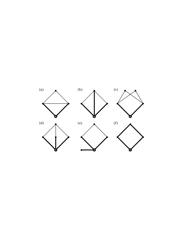
Figure 1. Examples of various PSP’s $S_{v}$ highlighted by thick edges. Note, in all cases except in case $(f)$ the set $F_{v}$ is empty and hence, the PSP’s $S_{v}$ in the other cases just contain the edges incident to $v$.

The reason why we call $S_{v}$ a partial star product is that $S_{v}$ is an isometric subgraph or even isomorphic to a Cartesian product graph $H$ of stars, as we shall see later (Theorem 3.9). Hence, $S_{v}$ is a partial product of $H$. For the construction of this graph $H$ we introduce the so-called star factors $\mathbb{S}_{i}$, see also Figures 1 and 3.

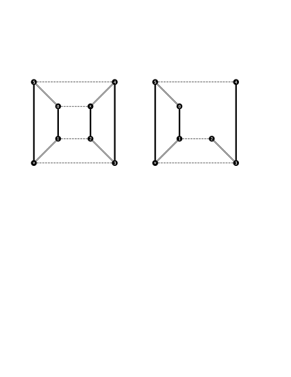
Figure 2. Left: A hypercube $Q_{3}$ is shown. The three equivalence classes of $\delta^{*}(Q_{3})$ are highlighted by solid, dashed and double lined edges, respectively. Right: The PSP $S_{v}$ is shown. Again, $\mathfrak{d}^{*}_{v|S_{v}}$ has three equivalence classes. However, since the edges $(0,1)$ and $(1,2)$ as well as the edges $(2,3)$ and $(3,4)$ span no square we can conclude that $\delta^{*}(S_{v})$ just contains one equivalence class. Hence, $\mathfrak{d}^{*}_{v|S_{v}}\neq\delta^{*}(S_{v})$ .

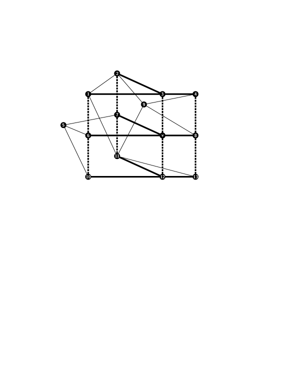
Figure 3. Shown is a graph $G\simeq\langle N^{G}_{2}[v]\rangle$. Note, $\delta(G)^{*}$ has one equivalence class and thus, $G$ is prime. However, the partial star product (PSP) $S_{v}$, that is the subgraph that consists of thick and dashed edges is not prime. The subgraph $S_{v}$ is isomorphic to the Cartesian Product of a star with four and a star with three vertices. The two equivalence classes of $\mathfrak{d}_{|S_{v}}$ are highlighted by thick, resp. dashed edges.

Definition 3.2 (Star Factor).

Let $G=(V,E)$ be an arbitrary given graph and $S_{v}$ be a PSP for some vertex $v\in V$. Assume $\mathfrak{d}_{v}^{*}$ has equivalence classes $\varphi_{1},\dots,\varphi_{n}$. We define the star factor $\mathbb{S}_{i}$ as the graph with vertex set $N_{\varphi_{i}}[v]$ that contains all primal edges of $E_{v}$ that are also in the induced closed $\varphi_{i}$-neighborhood, i.e., $E(\mathbb{S}_{i})=E(\langle N_{\varphi_{i}}[v]\rangle)\cap E_{v}$.

Note, this definition forbids triangles in $\mathbb{S}_{i}$, and hence, each $\mathbb{S}_{i}$ is indeed a star. We denote the restriction of $\mathfrak{d}^{*}_{v}$ to the subgraph $S_{v}$ with

$$\mathfrak{d}_{|S_{v}}:=\mathfrak{d}^{*}_{v|S_{v}}=\{(e,f)\in\mathfrak{d}^{*}_{v}\mid e,f\in E(S_{v})\}.$$

In other words, $\mathfrak{d}_{|S_{v}}$ is the subset of $\mathfrak{d}^{*}_{v}$ that contains all pairs of edges $(e,f)\in\mathfrak{d}^{*}_{v}$ where both edges $e$ and $f$ are contained in $S_{v}$. We want to emphasize that $\mathfrak{d}^{*}_{v|S_{v}}\neq\delta^{*}(S_{v})$; see Figure 2. In addition, by Lemma 2.5 we can conclude that $\mathfrak{d}_{|S_{v}}$ is an equivalence relation. For a given subset $W\subseteq V$ we define

$$\mathfrak{d}_{|S_{v}}(W)=\cup_{v\in W}\mathfrak{d}_{|S_{v}}$$

as the union of relations $\mathfrak{d}_{|S_{v}}$, $v\in W$. As it will turn out, for a given graph $G=(V,E)$ the transitive closure $\mathfrak{d}_{|S_{v}}(V)^{*}$ is the equivalence relation $\delta(G)^{*}$, see Theorem 3.11.

3.2. Properties of the Partial Star Product

We now establish basic properties of the graph $S_{v}$, its edge sets $E_{v}$ and $F_{v}$, as well as of the relation $\mathfrak{d}_{v}^{*}$ and its restriction $\mathfrak{d}_{|S_{v}}$ to $S_{v}$.

Lemma 3.3.

Given a graph $G=(V,E)$ and a vertex $v\in V$. Then $F_{v}=\emptyset$ if and only if for all edges $e,e^{\prime}\in E_{v}$ holds $(e,e^{\prime})\in\mathfrak{d}^{*}_{v}$. Moreover, if $F_{v}\neq\emptyset$ then $|F_{v}|\geq 2$.

Proof.

Clearly, if for all edges $e,e^{\prime}\in E_{v}$ holds $(e,e^{\prime})\in\mathfrak{d}^{*}_{v}$ then by definition $F_{v}=\emptyset$.

Let $F_{v}=\emptyset$ and assume there are edges $e,e^{\prime}\in E_{v}$ that are not in relation $\mathfrak{d}_{v}^{*}$. In particular, these edges are not in relation $\mathfrak{d}_{v}$, and therefore not in relation $\delta(G)$. By Condition $(i)$ of Def. 2.6 and since $e$ and $e^{\prime}$ are adjacent, there is a chordless square containing $e$ and $e^{\prime}$ and therefore, respective opposite edges $f$ and $f^{\prime}$. Condition $(ii)$ of Def. 2.6 implies $(e,f),(e^{\prime},f^{\prime})\in\delta(G)$. Therefore, $f,f^{\prime}\in F_{v}$, a contradiction.

Furthermore, since $F_{v}$ contains all opposite edges of squares spanned by $e,e^{\prime}\in E_{v}$ we can easily conclude that $|F_{v}|\geq 2$, if $F_{v}\neq\emptyset$. ∎

Lemma 3.4.

Let G=(V,E) be a given graph and let $S_{v}$ be a PSP for some vertex $v\in V$. If $e,f\in E_{v}$ are primal edges that are not in relation $\mathfrak{d}_{v}^{*}$, then $e$ and $f$ span a unique chordless square with a unique top vertex in $G$.

Conversely, suppose that $x$ is a non-primal vertex of $S_{v}$, then there is a unique chordless square in $S_{v}$ that contains vertex $x$ and that is spanned by edges $e,f\in E_{v}$ with $(e,f)\not\in\mathfrak{d}^{*}_{v}$.

Proof.

First, we show that $e$ and $f$ span a unique chordless square in $G$. By contraposition, assume $e$ and $f$ span no unique chordless square in $G$. Since $e$ and $f$ are adjacent, Condition $(i)$ of Def. 2.6 implies that $(e,f)\in\delta(G)$ and hence, $(e,f)\in\mathfrak{d}_{v}\subseteq\mathfrak{d}_{v}^{*}$. Therefore, if $(e,f)\notin\mathfrak{d}_{v}^{*}$, then they must span a unique chordless square. Let $e=(v,u)$ and $f=(v,w)$, $(e,f)\notin\mathfrak{d}_{v}^{*}$, span the unique chordless square $SQ_{1}=\langle\{v,u,x,w\}\rangle$ and assume for contradiction that the top vertex $x$ is not unique. Hence, there must be at least three squares: the square $SQ_{1}$, the square $SQ_{2}=\langle\{v,u,x,y\}\rangle$ spanned by $e$ and $g$, and the square $SQ_{3}=\langle\{v,w,x,y\}\rangle$ spanned by $f$ and $g=(v,y)$. We denote edges as follows: $a=(x,y)$ and $b=(x,w)$. Assume both squares $SQ_{2}$ and $SQ_{3}$ are chordless. Then Def. 2.6 $(ii)$ implies $(f,a),(a,e)\in\delta(G)$ and therefore, $(e,f)\in\mathfrak{d}_{v}^{*}$, a contradiction. If both squares have a chord then Def. 2.6 $(i)$ implies that $(e,g),(f,g)\in\delta(G)$ and thus, $(e,f)\in\mathfrak{d}_{v}^{*}$, again a contradiction. If only one square, say $SQ_{2}$, has a chord $(u,y)$, then $(e,g)\in\delta(G)$ and $(f,a),(g,a)\in\delta(G)$ and again we have $(e,f)\in\mathfrak{d}_{v}^{*}$.

Assume $x$ is a non-primal vertex in $S_{v}$. By definition, there are non-primal edges $f^{\prime}=(x,u),e^{\prime}=(x,w)\in F_{v}$ that are contained in a square spanned by $e=(v,u),f=(v,w)\in E_{v}$, whereas $(e,f)\not\in\mathfrak{d}_{v}^{*}$. As shown above, the square spanned by $e$ and $f$ is unique with unique top vertex in $G$ and therefore in $S_{v}$. Hence, if there is another square in $S_{v}$ containing $x$ then it must be spanned by $e^{\prime},f^{\prime}$ and this square contains additional edges $f^{\prime\prime}=(y,u),e^{\prime\prime}=(y,w)$. However, then there is a square $\langle\{v,u,y,w\}\rangle$, which contradicts the fact that the square spanned by $e$ and $f$ is unique. If the unique square spanned by $e$ and $f$ is not chordless in $G$, then Def. 2.6 $(i)$ implies $(e,f)\in\delta(G)$ and thus $(e,f)\in\mathfrak{d}_{v}^{*}$, a contradiction. ∎

By means of Lemma 3.3 and 3.4 and the definition of partial star products we can directly infer the next corollary.

Corollary 3.5.

Let G=(V,E) be a given graph and let $S_{v}$ be a PSP for some vertex $v\in V$.

1. If $(e,f)\in\mathfrak{d}_{v}^{*}$ then there is no square in $S_{v}$ spanned by $e$ and $f$.

2. Every square in $S_{v}$ contains two edges $e,e^{\prime}\in E_{v}$ and two edges $f,f^{\prime}\in F_{v}$, and every edge $f\in F_{v}$ is opposite to some primal edge $e\in E_{v}$.

3. Every non-primal vertex in $S_{v}$ is a unique top vertex of some square spanned by edges $e,e^{\prime}\in E_{v}$.

Lemma 3.6.

Let G=(V,E) be a given graph and let $f\in F_{v}$ be a non-primal edge of a PSP $S_{v}$ for some vertex $v\in V$. Then $f$ is opposite to exactly one primal edge $e\in E_{v}$ in $S_{v}$ and $(e,f)\in\mathfrak{d}_{|S_{v}}$.

Proof.

By Corollary 3.5, construction of $S_{v}$ and since $f\in F_{v}$, there is at least one edge $e\in E_{v}$ such that $f$ is opposite to $e$ and therefore at least one square $SQ_{1}=\langle\{v,w,x,u\}\rangle$ in $S_{v}$ spanned by primal edges $e=(v,u)$ and $e^{\prime}=(v,w)$ that contains the edge $f=(w,x)$. Note, by construction $(e,e^{\prime})\not\in\mathfrak{d}^{*}_{v}$ and $e$ is opposite to $f$. Assume for contradiction that $f$ is opposite to another edge $g=(v,y)$. Then there is another square $SQ_{2}=\langle\{v,y,x,w\}\rangle$. Hence, $e$ and $e^{\prime}$ do not span a square with unique top vertex in $G$. By Definition 2.6 and Lemma 3.4 we can conclude that $(e,e^{\prime})\in\mathfrak{d}^{*}_{v}$, a contradiction. Hence $e$ and $e^{\prime}$ span a unique chordless square containing the edge $f$. By Condition (i) of Definition 2.6 it holds $(e,f)\in\delta$. Since $e\in E_{v}$ we claim $(e,f)\in\mathfrak{d}_{v}$ and consequently $(e,f)\in\mathfrak{d}_{|_{S_{v}}}$. ∎

Lemma 3.7.

Let G=(V,E) be a given graph with maximum degree $\Delta$ and $W\subseteq V$ such that $\langle W\rangle$ is connected. Then each vertex $x\in W$ meets every equivalence class of $\mathfrak{d}_{|S_{v}}(W)^{*}$ in $\cup_{v\in W}S_{v}$, i.e., for each equivalence class $\varphi\mathrel{{{{}^{\boldsymbol{\sqsubseteq}}}}}\mathfrak{d}_{|S_{v}}(W)^{*}$ and for each vertex $x\in W$ there is an edge $(x,y)\in\varphi$ with $(x,y)\in E(\cup_{v\in W}S_{v})$. Moreover, $\mathfrak{d}_{|S_{v}}(W)^{*}$ has at most $\Delta$ equivalence classes.

Proof.

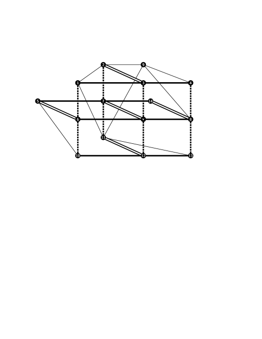
Figure 4. Shown is a graph $G\simeq\langle N^{G}_{2}[v]\rangle$. Note, $\delta(G)^{*}$ has one equivalence class. The partial star product (PSP) $S_{v}$ is the subgraph that consists of thick, double-lined and dashed edges. Moreover, $S_{v}$ can be isometrically embedded into the Cartesian product of a star with two and two stars with three vertices. The three equivalence classes of $\mathfrak{d}_{|S_{v}}$ are highlighted by thick, double-lined, resp. dashed edges.

Let $v\in W$ be an arbitrary vertex and $S_{v}$ be its PSP. We show first that $v$ meets every equivalence class of $\mathfrak{d}_{|S_{v}}$ in $S_{v}$. Assume for contradiction that there is an equivalence class $\varphi\mathrel{{{{}^{\boldsymbol{\sqsubseteq}}}}}\mathfrak{d}_{|S_{v}}$ that is not met by $v$ and hence for all edges $e\in E_{v}$ we have $e\not\in\varphi$. Hence, there must be a non-primal $f\in F_{v}$ with $f\in\varphi$. By construction of $S_{v}$ and by Lemma 3.6 this edge $f$ is opposite to exactly one edge $e\in E_{v}$ with $(e,f)\in\mathfrak{d}_{|S_{v}}$, but then $e\in\varphi$, a contradiction. We show now that every primal vertex $w$ in $S_{v}$ meets every equivalence class of $\mathfrak{d}_{|S_{v}}$. Let $\varphi\mathrel{{{{}^{\boldsymbol{\sqsubseteq}}}}}\mathfrak{d}_{|S_{v}}$ be an arbitrary equivalence class. If $e=(v,w)\in\varphi$ we are done. Therefore assume $e\not\in\varphi$. Hence, there must be at least a second equivalence class $\varphi^{\prime}\mathrel{{{{}^{\boldsymbol{\sqsubseteq}}}}}\mathfrak{d}_{|S_{v}}$ with $e\in\varphi^{\prime}$. Since vertex $v$ meets every equivalence class there is an edge $e^{\prime}=(v,u)\in\varphi$. Moreover, since $(e,e^{\prime})\not\in\mathfrak{d}_{v}^{*}$ it follows that $(e,e^{\prime})\not\in\mathfrak{d}_{v}\subseteq\delta$. Since $e$ and $e^{\prime}$ are adjacent and by Condition $(i)$ of Definition 2.6 the edges $e$ and $e^{\prime}$ span a unique chordless square. Hence, there is an opposite edge $f=(w,x)$ of $e^{\prime}$. By construction of $S_{v}$ we have $f\in F_{v}$ and hence, Lemma 3.6 implies $(e^{\prime},f)\in\mathfrak{d}_{|S_{v}}$. Therefore, the primal vertex $w$ meets equivalence class $\varphi$ in $S_{v}$. Note, not every equivalence class of $\mathfrak{d}_{|S_{v}}$ must be met by non-primal vertices in $S_{v}$ in general, as one can easily verify by the example in Figure 4.

It remains to show that every vertex $x\in W$ meets every equivalence class of $\mathfrak{d}_{|S_{v}}(W)^{*}$ in $\cup_{v\in W}S_{v}$. Assume we have chosen an arbitrary vertex $x\in W$, computed $S_{x}$ and $\mathfrak{d}_{|S_{x}}$. As shown, vertex $x$ and all its primal neighbors $y$ in $S_{x}$ meet every equivalence class of $\mathfrak{d}_{|S_{x}}$. Assume $W$ contains more than one vertex. Since $\langle W\rangle$ is connected there is a primal vertex $y$ of $x$ that is also contained in $W$. Hence, vertex $x$ is a primal neighbor of $y$ in $S_{y}$ and every equivalence class of $\mathfrak{d}_{|S_{y}}$ is met by $y$ as well as by $x$. Let $\varphi\mathrel{{{{}^{\boldsymbol{\sqsubseteq}}}}}(\mathfrak{d}_{|S_{x}}\cup\mathfrak{d}_{|S_{y}})^{*}$ be an arbitrary equivalence class. Assume neither $x$ nor $y$ meets $\varphi$. Then each edge $f\in\varphi$ must be in $F_{x}$ or $F_{y}$. Assume $f\in F_{y}$ then, by construction of $S_{y}$ and Lemma 3.6, this edge $f$ is opposite to exactly one edge $e\in E_{y}$ with $(e,f)\in\mathfrak{d}_{|S_{y}}$, and hence $e\in\varphi$, a contradiction. Assume now all edges $e\in\varphi$ are only met by $y$ but not by $x$, and therefore, $e^{\prime}=(x,y)\not\in\varphi$. However, since $e$ and $e^{\prime}$ are in different equivalence classes of $(\mathfrak{d}_{|S_{x}}\cup\mathfrak{d}_{|S_{y}})^{*}$ they must be in different equivalence classes of $\mathfrak{d}_{|S_{y}}$. Hence, $(e,e^{\prime})\not\in\mathfrak{d}^{*}_{y}$ and thus, $(e,e^{\prime})\not\in\mathfrak{d}_{y}\subseteq\delta$. Since $e$ and $e^{\prime}$ are adjacent and, by Condition $(i)$ of Definition 2.6, the edges $e$ and $e^{\prime}$ span a unique chordless square. Hence, there is an opposite edge $f=(x,w)$ of $e$ in $S_{y}$ and, by Lemma 3.6 we conclude $(e,f)\in\mathfrak{d}_{|S_{y}}$ and therefore, $f\in\varphi$, which implies that $x$ meets $\varphi$, a contradiction. Hence, every equivalence class $\varphi\mathrel{{{{}^{\boldsymbol{\sqsubseteq}}}}}(\mathfrak{d}_{|S_{x}}\cup\mathfrak{d}_{|S_{y}})^{*}$ must be met by $x$ and $y$. By the same arguments one shows that each primal vertex of $S_{x}$ and $S_{y}$ meets every equivalence class of $(\mathfrak{d}_{|S_{x}}\cup\mathfrak{d}_{|S_{y}})^{*}$. If $W\setminus\{x,y\}\neq\emptyset$ we can choose a primal neighbor $z\in W$ of $x$ or $y$, since $\langle W\rangle$ is connected. By the same arguments as before, one shows that each vertex $x,y$, resp. $z$ and each of its primal vertices in $S_{x},S_{y}$, resp. $S_{z}$ meets every equivalence class of $((\mathfrak{d}_{|S_{x}}\cup\mathfrak{d}_{|S_{y}})^{*}\cup\mathfrak{d}_{|S_{z}})^{*}=(\mathfrak{d}_{|S_{x}}\cup\mathfrak{d}_{|S_{y}}\cup\mathfrak{d}_{|S_{z}})^{*}$ in $S_{x}\cup S_{y}\cup S_{z}$. Therefore, we can traverse $\langle W\rangle$ in breadth-first search order and inductively conclude that every vertex $x\in W$ meets every equivalence class of $\mathfrak{d}_{|S_{v}}(W)^{*}$ in $\cup_{v\in W}S_{v}$.

Finally, we observe that each edge in $E_{v}$ might define one equivalence class of $\mathfrak{d}_{|S_{v}}$ for each vertex $v\in W$. Thus, $\mathfrak{d}_{|S_{v}}$ can have at most $\Delta$ equivalence classes. Since this holds for all vertices and since equivalence classes in $\mathfrak{d}_{|S_{v}}(W)^{*}$ are combined equivalence classes of the respective $\mathfrak{d}_{|S_{v}}$ classes, the number of equivalence classes in $\mathfrak{d}_{|S_{v}}(W)^{*}$ can not exceed $\Delta$. ∎

In order to prove that each PSP can be isometrically embedded into a Cartesian product of stars, which is shown in the next theorem, we first need the following lemma.

Lemma 3.8.

Let $G=\Box_{i=1}^{l}G_{i}$ be the Cartesian product of stars. Assume the vertices in each $V(G_{i})$ are labeled from $0,\dots,|V(G_{i})|-1$, where the vertex with label $0$ always denotes the star-center of each $G_{i}$. Let $v_{G}$ be the vertex with coordinates $c(v_{G})=(0,\dots,0)$ Then for any integer $k\geq 0$, the induced closed $k$-neighborhood $\langle N_{k}^{G}[v_{G}]\rangle$ is an isometric subgraph of $G$.

Proof.

Let $\langle N_{k}^{G}[v_{G}]\rangle$ be the induced closed $k$-neighborhood of $v_{G}$ in $G$. Let $x,y\in N_{k}^{G}[v_{G}]$ be arbitrary vertices and let $I\subseteq\{1,\dots,l\}$ be the set of positions where $x$ and $y$ differ in their coordinate. Moreover, let $I_{0}\subseteq I$ be the set of positions where either $x$ or $y$ has coordinate $0$. By the Distance Lemma we have $d_{G}(x,y)=\sum_{i\in I_{O}}1+\sum_{i\in I\setminus I_{O}}2$.

We now construct a path from $x$ to $y$ that is entirely contained in $N_{k}^{G}[v_{G}]$ and show that this path is a shortest path. Set $P(x,y)=\emptyset$. Let $i\in I_{0}$ and w.l.o.g. assume $c_{i}(x)=0$, otherwise we would interchange the role of $x$ and $y$. By definition of the Cartesian product there is a vertex $y^{\prime}$ that is adjacent to vertex $y$ with $c_{j}(y^{\prime})=c_{j}(y)$ for all $j\neq i$ and $c_{i}(y^{\prime})=0$. By the Distance Lemma, we have $d_{G_{j}}(c_{j}(v_{G}),c_{j}(y))=d_{G_{j}}(c_{j}(v_{G}),c_{j}(y^{\prime}))$ for all $j\neq i$ and $d_{G_{i}}(c_{i}(v_{G}),c_{i}(y))=d_{G_{i}}(0,c_{i}(y))=1$ and $d_{G_{i}}(c_{i}(v_{G}),c_{i}(y^{\prime}))=0$ and thus, $d_{G}(v_{G},y^{\prime})<d_{G}(v_{G},y)\leq k$, which implies that $y^{\prime}\in N_{k}^{G}[v_{G}]$. We assign $(y,y^{\prime})$ to be an edge of the (so far empty) path $P(x,y)$ from $x$ to $y$ and repeat to construct parts of the path from $x$ to $y^{\prime}$ in the same way until all $i\in I_{0}$ are processed. In this way, we constructed subpaths $P(x,v)$ and $P(w,y)$ of $P(x,y)$, both of which are entirely contained in $\langle N_{k}^{G}[v_{G}]\rangle$ and $|P(x,v)|+|P(w,y)|=|I_{0}|$. We are left to construct a path from $v$ to $w$ that is entirely contained in $N_{k}^{G}[v]$. Note that by construction $v$ and $w$ differ only in the $i$-th position of their coordinates where $i\in I\setminus I_{0}$ and $c_{j}(v)=c_{j}(x)=c_{j}(y)=c_{j}(w)$ for all $j\not\in I\setminus I_{0}$. By the definition of the Cartesian product for each $i\in I\setminus I_{0}$ there are edges $(v,v^{\prime})$, resp. $(v^{\prime},v^{\prime\prime})$ such that $v,v^{\prime}$ and $v^{\prime\prime}$ differ only in the $i$-th position of their coordinates. Since $0\neq c_{i}(x)=c_{i}(v)$ and by definition of the Cartesian product it follows that $c_{i}(v^{\prime})=0$ and $v^{\prime\prime}$ can be chosen such that $c_{i}(v^{\prime\prime})=c_{i}(y)=c_{i}(w)\neq 0$. By the Distance Lemma and the same arguments as used before it holds $d_{G}(v_{G},v^{\prime})=d_{G}(v_{G},v^{\prime\prime})-1=d_{G}(v_{G},v)-1\leq k$ and hence, $v^{\prime},v^{\prime\prime}\in N_{k}^{G}[v_{G}]$. Therefore we add the edges $(v,v^{\prime})$, resp. $(v^{\prime},v^{\prime\prime})$ to the path from $x$ to $y$, remove $i$ from $I\setminus I_{0}$ and repeat this construction for a path from $v^{\prime\prime}$ to $w$ until $I\setminus I_{0}$ is empty.

Hence we constructed a path of length $|I_{0}|+2|I\setminus I_{0}|=\sum_{i\in I_{O}}1+\sum_{i\in I\setminus I_{O}}2=d_{G}(x,y)$. Thus, this path is a shortest path from $x$ to $y$. Since this construction can be done for any $x,y\in N_{k}^{G}[v_{G}]$ we can conclude that $\langle N_{k}^{G}[v_{G}]\rangle$ is an isometric subgraph of $G$. ∎

Theorem 3.9.

Let $G=(V,E)$ be an arbitrary given graph and $S_{v}$ be a PSP for some vertex $v\in V$. Let $H=\Box_{i=1}^{k}\mathbb{S}_{i}$ be the Cartesian product of the star factors as in Definition 3.2. Then it holds:

1. $S_{v}$ is an isometric subgraph of $H$ and in particular, $S_{v}\simeq\langle N^{H}_{2}[(v_{1},\dots,v_{k})]\rangle$ where $v_{i}$ denotes the star-center of $\mathbb{S}_{i}$, $i=1,\dots,k$.

2. $\mathfrak{d}_{|S_{v}}\subseteq\delta(H)^{*}\subseteq\sigma(H)$.

3. The product relation $\sigma(H)$ has the same number of equivalence classes as $\mathfrak{d}_{|S_{v}}$.

Proof.

Assertion (1):
If $\mathfrak{d}_{v}^{*}$ has only one equivalence class, then there is nothing to show, since $S_{v}\simeq\mathbb{S}_{1}\simeq H$. Therefore, assume $\mathfrak{d}_{v}^{*}$ has $k\geq 2$ equivalence classes.

In the following we define a mapping $\gamma:V(S_{v})\rightarrow V(H)$ and show that $\gamma$ is an isometric embedding. In particular we show that $\gamma$ is an isomorphism from $S_{v}$ to the $2$-neighborhood $\langle N_{2}^{H}[v_{H}]\rangle$ for a distinguished vertex $v_{H}\in V(H)$. Lemma 3.8 implies then that this embedding is isometric.

For a given equivalence class $\varphi_{i}\mathrel{{{{}^{\boldsymbol{\sqsubseteq}}}}}\mathfrak{d}_{v}^{*}$ let $N_{\varphi_{i}}(v)=\{v_{1},\dots,v_{l}\}$ be the $\varphi_{i}$-neighborhood of the center $v$ and $\mathbb{S}_{i}$ be the corresponding star factor with vertex set $V(\mathbb{S}_{i})=\{0,1,\dots,l\}$ and edges $(0,x)\in E(\mathbb{S}_{i})$ for all $(v,v_{x})\in S_{v}$. Let $H=\Box_{i=1}^{k}\mathbb{S}_{i}$ be the Cartesian product of the star factors. The center $v$ of $S_{v}$ is mapped to the vertex $v_{H}\in V(H)$ with coordinates $c(v_{H})=(0,\dots,0)$, the vertices $v_{j}\in N_{\varphi_{i}}(v)$ are mapped to the unique vertex $u$ with coordinates $c_{r}(u)=0$ for all $r\neq i$ and $c_{i}(u)=j$. Clearly, these vertices exist, due to the construction of $\mathbb{S}_{1},\dots,\mathbb{S}_{k}$ and since $V(H)=\times_{i=1}^{k}V(\mathbb{S}_{i})$. Note, that these vertices we mapped onto are entirely contained in the 1-neighborhood $N^{H}[v_{H}]$ of $v_{H}$. Now let $x$ be a non-primal vertex in $S_{v}$. Hence, by Lemma 3.4 and Corollary 3.5, there is a unique chordless square $\langle\{v,v_{i},x,v_{j}\}\rangle$ in $S_{v}$ with unique top vertex $x$. Thus, $v_{i}$ and $v_{j}$ are the only common neighbors of $x$ in $S_{v}$. Moreover, by definition and Lemma 3.4, the edges $(v,v_{i})\in\varphi_{r}$ and $(v,v_{j})\in\varphi_{s}$ are in different equivalence classes, i.e., $r\neq s$. Thus, we map $x$ to the unique vertex $u$ with coordinates $c_{l}(u)=0$ for all $l\neq r,s$ and $c_{r}(u)=i$ and $c_{s}(u)=j$. Again, this vertex exists, due to the construction of $\mathbb{S}_{1},\dots,\mathbb{S}_{k}$ and since $V(H)=\times_{i=1}^{k}V(\mathbb{S}_{i})$. This completes the construction of our mapping $\gamma$.

We continue to show that the mapping $\gamma:V(S_{v})\rightarrow N_{2}^{H}[v_{H}]$ is bijective. It is easy to see that by construction and the definition of the Cartesian product, each primal vertex $x$ has a unique partner $\gamma(x)$ in $N_{1}^{H}[v_{H}]$ and vice versa. We show that this holds also for non-primal vertices in $S_{v}$ and vertices in $N_{2}^{H}[v_{H}]\setminus N_{1}^{H}[v_{H}]$. First assume there are two non-primal vertices $x$ and $x^{\prime}$ in $S_{v}$ that are mapped to the same vertex $u$ in $H$. Thus, by construction of our mapping $\gamma$, the vertex $x^{\prime}$ must have the same primal neighbors $v_{i}$ and $v_{j}$ as $x$ in $S_{v}$. However, by Lemma 3.4 this contradicts that $(v,v_{i})\in\varphi_{r}$ and $(v,v_{j})\in\varphi_{s}$ span a unique square. Therefore, $\gamma$ is injective. Now, let $u\in N_{2}^{H}[v_{H}]\setminus N_{1}^{H}[v_{H}]$ be an arbitrary vertex in $H$. By the Distance Lemma we can conclude that $d_{H}(v_{H},u)=\sum_{i=1}^{k}d_{\mathbb{S}_{i}}(0,c_{i}(u))$. Moreover, since $d_{H}(v_{H},u)=2$ and $d_{\mathbb{S}_{i}}(0,c_{i}(u))\leq 1$ for all $i=1,\dots,k$ we can conclude that $d_{H}(v_{H},u)=d_{\mathbb{S}_{r}}(0,c_{r}(u))+d_{\mathbb{S}_{s}}(0,c_{s}(u))$ for some distinct indices $r$ and $s$. Assume that $c_{r}(u)=i$ and $c_{s}(u)=j$. By construction, the star factor $\mathbb{S}_{r}$ contains the edge $(0,i)$ and $\mathbb{S}_{s}$ the edge $(0,j)$. Hence, there are edges $e=(v,v_{i})\in\varphi_{r}$ and $f=(v,v_{j})\in\varphi_{s}$ in $S_{v}$. Lemma 3.4 implies that there is a unique chordless square spanned by $e$ and $f$ with unique top vertex $y$ that is also contained in $S_{v}$. By construction of $\gamma$ the vertex $y$ is the unique vertex that is mapped to vertex $u$ in $H$. Since this holds for all vertices $u\in N_{2}^{H}[v_{H}]\setminus N_{1}^{H}[v_{H}]$, and by the preceding arguments, we can conclude that the mapping $\gamma:S_{v}\rightarrow N_{2}^{H}[v_{H}]$ we defined is bijective.

It remains to show that $\gamma$ is an isomorphism from $S_{v}$ to $N_{2}^{H}[v_{H}]$. By construction, every primal edge $(v,v_{j})\in\varphi_{r}$ is mapped to the edge $(v_{H},x)$, where $x$ has coordinates $c_{i}(x)=0$ for $i\neq r$ and $c_{r}(x)=j$. Hence, $(v,v_{j})\in E_{v}$ if and only if $(\gamma(v),\gamma(v_{j}))\in E(\langle N_{2}^{H}[v_{H}]\rangle)$. Now suppose we have a non-primal edge $(v_{j},y)\in\varphi_{r}$. By Lemma 3.4, there is a unique chordless square with edges $(v,v_{l})\in\varphi_{r}$ and $(v,v_{j})\in\varphi_{s}$ and hence, by construction of $\mathbb{S}_{r}$ and $\mathbb{S}_{s}$ and the definition of the Cartesian product, there are edges $e=(v_{H},z)$ and $f=(v_{H},z^{\prime})$ in $H$ where $z$ differs from $v_{H}$ in the $r$-th position of its coordinate and $z^{\prime}$ differs from $v_{H}$ in the $s$-th position of its coordinate. By the Square Property, there is unique chordless square in $H$ spanned by $e$ and $f$ with top vertex $y^{\prime}$ that has coordinates $c_{i}(y^{\prime})=0$ for $i\neq r,s$, $c_{r}(y^{\prime})=l\neq 0$ and $c_{s}(y^{\prime})=j\neq 0$. By the construction of $\gamma$ we see that $(v_{j},y)\in F_{v}$ implies $(\gamma(v_{j}),\gamma(y))=(z^{\prime},y^{\prime})\in E(\langle N_{2}^{H}[v_{H}]\rangle)$. Using the same arguments, but starting from squares spanned by $e=(v_{H},z)$ and $f=(v_{H},z^{\prime})$ in $H$, one can easily derive that $(z^{\prime},y^{\prime})\in E(\langle N_{2}^{H}[v_{H}]\rangle)$ implies $(\gamma^{-1}(z^{\prime}),\gamma^{-}1(y^{\prime}))=(v_{j},y)\in F_{v}$.

Finally, Lemma 3.8 implies that $\langle N_{2}^{H}[v_{H}]\rangle$ is an isometric subgraph of $H$ and therefore, $\gamma:V(S_{v})\rightarrow V(H)$ is an isometric embedding.

Assertion (2) and (3):
By Assertion (1), we can treat the graph $S_{v}$ as subgraph of $H$; $S_{v}\subseteq H$. We continue to show that $\mathfrak{d}_{|S_{v}}=\mathfrak{d}^{*}_{v|S_{v}}\subseteq\delta(H)^{*}$. Let $v\in V(G)$ be the center of the PSP $S_{v}$, and $H=\Box_{i=1}^{k}\mathbb{S}_{i}$, where $\mathbb{S}_{i}$ are the corresponding star factors (w.r.t. $S_{v}$). Let $e,f\in E(S_{v})$ such that $(e,f)\in\mathfrak{d}_{|S_{v}}$. There are three cases to consider; either $e,f\in E_{v}$, or $e,f\in F_{v}$, or $e\in E_{v}$ and $f\in F_{v}$.

If $e,f\in E_{v}$ are both primal edges with $(e,f)\in\mathfrak{d}_{|S_{v}}$ then $e$ and $f$ are by construction of the star factors and $H$ contained in the layer $\mathbb{S}_{i}^{v}$ of some star factor $\mathbb{S}_{i}$. Corollary 3.5 and $(e,f)\in\mathfrak{d}_{|S_{v}}\subseteq\mathfrak{d}_{v}^{*}$ imply that $e$ and $f$ span no square in $S_{v}$. Since $H=\Box_{i=1}^{k}\mathbb{S}_{i}$ we can conclude that $e$ and $f$ span no square in $H$ and hence, $(e,f)\in\delta(H)$.

Assume $e,f\in F_{v}$ and $(e,f)\in\mathfrak{d}_{|S_{v}}$. By Lemma 3.6 it holds that $e$, resp., $f$ is opposite to exactly one primal edge $e^{\prime}\in E_{v}$, resp., $f^{\prime}\in E_{v}$ in $S_{v}$ where $(e,e^{\prime}),(f,f^{\prime})\in\mathfrak{d}_{|S_{v}}$. Since $S_{v}\subseteq H$, the edge $e$ is the opposite edge of $e^{\prime}$ and $f$ is the opposite edge of $f^{\prime}$ in a square which is also contained in $H$. Since $S_{v}$ is an isometric subgraph of $H$ we can conclude that this square is chordless in $H$ and thus $(e,e^{\prime}),(f,f^{\prime})\in\delta(H)$. Since $\mathfrak{d}_{|S_{v}}$ is transitive it holds, $(e^{\prime},f^{\prime})\in\mathfrak{d}_{|S_{v}}$. By analogous arguments as before we have $(e^{\prime},f^{\prime})\in\delta(H)$ and therefore, $(e,f)\in\delta^{*}(H)$.

Finally, suppose $e\in E_{v}$ is a primal edge, $f\in F_{v}$ is non-primal and $(e,f)\in\mathfrak{d}_{|S_{v}}$. By Lemma 3.6, $f$ is opposite to exactly one primal edge $e^{\prime}$ where $(f,e^{\prime})\in\mathfrak{d}_{|S_{v}}$. If $e=e^{\prime}$, then $e$ and $f$ are opposite edges in a chordless square in $S_{v}$. By analogous arguments as before, we can conclude that this square is chordless in $H$ and hence, $e,f\in\delta(H)$. If $e\neq e^{\prime}$, then $(e,f),(f,e^{\prime})\in\mathfrak{d}_{|S_{v}}$ implies that $(e,e^{\prime})\in\mathfrak{d}_{|S_{v}}$ and we can conclude from Corollary 3.5 that there is no square spanned by $e$ and $e^{\prime}$ in $S_{v}$. Again $e$ and $e^{\prime}$ lie in common layer $\mathbb{S}_{i}^{v}$ and do not span any square in $H$. Thus we have $(e,e^{\prime})\in\delta(H)$. Again, since $e^{\prime}$ and $f$ are opposite edges in a chordless square in $H$ we can conclude that $(e^{\prime},f)\in\delta(H)$. Consequently, $\mathfrak{d}_{|S_{v}}\subseteq\delta^{*}(H)$. Note, by results of Imrich [18] we have $\delta(H)^{*}\subseteq\sigma(H)$. It is easy to see that the connected components of $\delta(H)^{*}$ w.r.t. to a fixed equivalence class $i$ correspond to the layers of the factor $\mathbb{S}_{i}$. Therefore, we can conclude that $\delta(H)^{*}=\sigma(H)$. Hence, we have

$$\mathfrak{d}_{|S_{v}}=\mathfrak{d}^{*}_{v|S_{v}}\subseteq\delta(H)^{*}=\sigma(H).$$

Moreover, by Definition 3.2 of the star factors and since stars are prime, the number of $\mathfrak{d}_{|S_{v}}$ classes equals the number of prime factors of $H$. Hence, it holds that $\mathfrak{d}_{|S_{v}}$ and $\sigma(H)$ have the same number of equivalence classes. ∎

By the construction of star factors, the Distance Lemma and Theorem 3.9, we can directly infer the next corollary.

Corollary 3.10.

Let $G=(V,E)$ be an arbitrary given graph, $S_{v}$ be a PSP for some vertex $v\in V$ and $\mathfrak{d}_{v}^{*}$ have $k=1$ or $2$ equivalence classes. Then

$$S_{v}\simeq\Box_{i=1}^{k}\mathbb{S}_{i}.$$

We conclude this section with a last theorem which shows that the transitive closure of the union $\mathfrak{d}_{|S_{v}}(V)$ over all vertices and its relations $\mathfrak{d}_{v}$, even restricted to $S_{v}$, is $\delta(G)^{*}$.

Theorem 3.11.

Let $G=(V,E)$ be a given graph and $\mathfrak{d}_{|S_{v}}(V)=\cup_{v_{\in}V}\mathfrak{d}_{|S_{v}}$. Then

$$\mathfrak{d}_{|S_{v}}(V)^{*}=\delta(G)^{*}.$$

Proof.

By definition $\mathfrak{d}_{v}\subseteq\delta(G)$. Moreover, by definition and Lemma 2.5 it holds that $\mathfrak{d}_{|S_{v}}\subseteq\mathfrak{d}_{v}^{*}\subseteq\delta(G)^{*}$ for all $v\in V(G)$. Thus, $\mathfrak{d}_{|S_{v}}(V)\subseteq\delta(G)^{*}$, and hence $\mathfrak{d}_{|S_{v}}(V)^{*}\subseteq\delta(G)^{*}$.

Let $e,f\in E(G)$ be edges that are in relation $\delta(G)$. By definition, $(e,f)\in\mathfrak{d}_{v}$ for some $v\in V(G)$. If $e=(u,v)$ and $f=(w,v)$ are adjacent, then $e$ and $f$ are contained in the set $E_{v}$ of $S_{v}$ and therefore in $\mathfrak{d}_{|S_{v}}\subseteq\delta(G)^{*}$. Assume, $e=(u,v)$ and $f=(x,y)$ are opposite edges of a chordless square containing the edges $e,f$ and $g=(v,x)$. For contradiction, assume $(e,f)\not\in\mathfrak{d}_{|S_{v}}(V)^{*}$ and hence $(e,f)\not\in\mathfrak{d}_{|S_{v}}(V)$. Thus, for each $v\in V$ we have $(e,f)\not\in\mathfrak{d}_{|S_{v}}$ and therefore, by definition, there is no square spanned by edges $e,e^{\prime}\in E_{v}$ with $(e,e^{\prime})\not\in\mathfrak{d}_{v}^{*}$ such that $f$ is the opposite edge of $e$. In particular, this implies $(e,g)\in\mathfrak{d}_{v}^{*}$ and hence $(e,g)\in\mathfrak{d}_{|S_{v}}$. Analogously, one shows that $(f,g)\in\mathfrak{d}_{|S_{x}}$. Since $\mathfrak{d}_{|S_{v}}\cup\mathfrak{d}_{|S_{x}}\subseteq\mathfrak{d}_{|S_{v}}(V)$ we can infer that $(e,f)\in\mathfrak{d}_{|S_{v}}(V)^{*}$, a contradiction. ∎

Theorem 3.11 allows us to provide covering algorithms for the recognition of $\delta(G)^{*}$ or of $\delta(H)^{*}$ for subgraphs $H\subseteq G$ that are based only on coverings by partial star products. Note, if $\sigma(G)=\delta(G)^{*}$, then the covering of $G$ by partial star products would also lead to a valid prime factorization. However, as most graphs are prime we will in the next section provide algorithms, based on factorizable parts, i.e., of coverings where the PSP’s have more than one equivalence class $\mathfrak{d}_{|S_{v}}$, which can be used to recognize approximate products.

4. Recognition of Relations, Colorings and Embeddings into Cartesian Products

In order to compute local colorings based on partial star products and to compute coordinates that respect this coloring we begin with algorithms for the recognition of $\mathfrak{d}_{|S_{v}}(W)^{*}$ and $\delta(G)^{*}$.

Lemma 4.1.

Given a graph $G=(V,E)$ with maximum degree $\Delta$ and a subset $W\subseteq V$ such that $\langle W\rangle$ is connected, then Algorithm 1 computes $\mathfrak{d}_{|S_{v}}(W)^{*}$ and $\cup_{v\in W}S_{v}$ in $O(|V|\Delta^{4})$ time.

Proof.

The Algorithm scans the vertices in an arbitrary order and computes $\langle N_{2}^{G}[v]\rangle$, $\delta^{\prime}=\delta(\langle N_{2}^{G}[v]\rangle)$, as well as $S_{v}$ and $\mathfrak{d}_{|S_{v}}$ w.r.t. $\delta^{\prime}$. In order to compute the transitive closure of $\mathfrak{d}_{|S_{v}}(W)$ an auxiliary graph, the color graph $\Gamma$, is introduced. For each vertex $v$ and to each equivalence class of $\mathfrak{d}_{|S_{v}}$ some unique color is assigned, and $\Gamma$ keeps track of the “colors” of the equivalence classes. All vertices of $\Gamma$ are pairs $(e,c)$. Two vertices $(e^{\prime},c^{\prime})$ and $(e^{\prime\prime},c^{\prime\prime})$ are connected by an edge if and only if there is an edge $e\in\varphi_{c^{\prime}}\cap\varphi_{c^{\prime\prime}}$ with $\varphi_{c^{\prime}}\mathrel{{{{}^{\boldsymbol{\sqsubseteq}}}}}\mathfrak{d}_{|S_{u}}$ and $\varphi_{c^{\prime\prime}}\mathrel{{{{}^{\boldsymbol{\sqsubseteq}}}}}\mathfrak{d}_{|S_{w}}$ for some $u,w\in W$. In other words, if there is an edge $e$ that obtained both, color $c^{\prime}$ and $c^{\prime\prime}$. Edges in $\Gamma$ “connect” edges of local equivalence classes that belong to the same global equivalence classes in $\mathfrak{d}_{|S_{v}}(W)^{*}$. The connected components $Q$ of $\Gamma$ define edge sets $E_{Q}=\cup_{(e,c)\in Q}\varphi_{c}$. We therefore can identify the transitive closure of $\mathfrak{d}_{|S_{v}}(W)^{*}$ by defining $e\in\varphi_{Q}\mathrel{{{{}^{\boldsymbol{\sqsubseteq}}}}}\mathfrak{d}_{|S_{v}}(W)^{*}$ if $e\in E_{Q}$. Finally, we observe that this is iteratively done for all vertices $v\in W$, that all edges in $E(\langle W\rangle)$ are contained in some $E_{v}$ of $S_{v}$ and, by Lemma 3.7, that every equivalence class of $\mathfrak{d}_{|S_{v}}(W)^{*}$ is met by every vertex $v\in W$. Therefore, we can conclude that each edge is uniquely assigned to some class $\varphi_{Q}\mathrel{{{{}^{\boldsymbol{\sqsubseteq}}}}}\mathfrak{d}_{|S_{v}}(W)^{*}$. Hence, the algorithm is correct.

In order to determine the time complexity we first consider line 6. The induced $2$-neighborhood can be computed in $\Delta^{2}$ time and has at most $\Delta^{2}$ vertices, and hence at most $\Delta^{4}$ edges. As shown by Chiba and Nishizeki [2] all triangles and all squares in a given graph $G=(V,E)$ can be computed in $O(|E|\Delta)$ time. Combining these results, we can conclude that all chordless squares can be listed in $O(|E|\Delta)$ time. Thus, in this preprocessing step, we are able to determine $\delta^{\prime},S_{v}$ and $\mathfrak{d}_{|S_{v}}$ in $O(\Delta^{4})$ time. Since this is done for all vertices $v\in W$, we end in an overall time complexity $O(|E|\Delta+|W|\Delta^{4})$ for the preprocessing step and the while-loop. For the second part, we observe that $\Gamma$ has at most $O(|E|)$ connected components. Since the number of edges is bounded by $|V|\Delta$ we conclude that Algorithm 1 has time complexity $O(|V|\Delta^{2}+|W|\Delta^{4})=O(|V|\Delta^{4})$. ∎

Algorithm 1 Local $\mathfrak{d}_{|S_{v}}(W)^{*}$ computation

1:  INPUT: A graph $G=(V,E)$, $W\subseteq V$.

2:  $\sigma\leftarrow W$

3:  initialize graph $\Gamma=\emptyset$; {called “color graph”}

4:  while $\sigma\neq\emptyset$ do

5:     take any vertex $v$ of $\sigma$;

6:     compute $\langle N_{2}^{G}[v]\rangle$, $\delta^{\prime}=\delta(\langle N_{2}^{G}[v]\rangle)$, $S_{v}$ and $\mathfrak{d}^{*}_{|S_{v}}$ w.r.t. $\delta^{\prime}$;

7:     color the edges of $S_{v}$ w.r.t. the equivalence classes of $\mathfrak{d}_{|S_{v}}$;

8:     set $num\_class$ = the number of equivalence classes of $\mathfrak{d}_{|S_{v}}$;

9:     add $num\_class$ new vertices to $\Gamma$;

10:     for every edge $e$ in $S_{v}$ do

11:        if $e$ was already colored in $G$ then

12:           x = old color of $e$; y = new color of $e$;

13:           add vertices $(x,e)$ and $(y,e)$ to $\Gamma$

14:           join all vertices of the from $(x,f)$ and $(y,f^{\prime})$ in $\Gamma$;

15:        end if

16:     end for

17:     delete $v$ from $\sigma$;

18:  end while

19:  {compute the equivalence class $\varphi_{k}\mathrel{{{{}^{\boldsymbol{\sqsubseteq}}}}}\mathfrak{d}_{|S_{v}}(W)^{*}$.}

20:  set $num\_comp$ = number of connected components of $\Gamma$;

21:  for $k=1$ to $num\_comp$ do

22:     if color of $e$ is vertex in component $k$ of $\Gamma$ then

23:        $\varphi_{k}\leftarrow e$;

24:     end if

25:  end for

26:  OUTPUT: $\mathfrak{d}_{|S_{v}}(W)^{*}$ and $\cup_{v\in W}S_{v}$;

By means of Theorem 3.11 and Lemma 4.1 we can directly infer the next corollary.

Corollary 4.2.

Let $G=(V,E)$ be a given graph with maximum degree $\Delta$. Then $\delta(G)^{*}$ can be computed in $O(|V|\Delta^{4})$ time by a call of Algorithm 1 with input $G$ and $W=V$.

As mentioned before, a vertex $x$ of a Cartesian product $\Box_{i=1}^{n}G_{i}$ is properly “coordinatized” by the vector $c(x):=(c_{1}(x),\dots,c_{n}(x))$, whose entries are the vertices $c_{i}(x)$ of its factor graphs $G_{i}$. Two adjacent vertices in a Cartesian product graph differ in exactly one coordinate. Furthermore, the coordinatization of a product is equivalent to an edge coloring of $G$ in that edges $(x,y)$ share the same color $c_{k}$ if $x$ and $y$ differ in the coordinate $k$. This colors the edges of $G$ (with respect to the given product representation).

Conversely, the idea of Algorithm 2 is to compute vertex coordinates of a subgraph of $\cup_{v\in W}S_{v}$ based on its $\mathfrak{d}_{|S_{v}}(W)^{*}$-coloring. In particular, we want to compute coordinates that reflect parts of the $\mathfrak{d}_{|S_{v}}(W)^{*}$-coloring of $\cup_{v\in W}S_{v}$ in a consistent way. Consistent means that all adjacent vertices $u$ and $v$ with $(u,v)\in\varphi_{r}\mathrel{{{{}^{\boldsymbol{\sqsubseteq}}}}}\mathfrak{d}_{|S_{v}}(W)^{*}$ differ exactly in their $r$-th position of their coordinate vectors, and no two distinct vertices obtain the same coordinate. This goal cannot always be achieved for all vertices contained in $\cup_{v\in W}S_{v}$. In [8, p. 280 et seqq.] a way is shown how to avoid those inconsistencies. In this approach colors of edges with “inconsistent” vertices are merged to one color. However, if the graph under investigation is only slightly perturbed, but prime, this approach would merge all colors to one. This is what we want to avoid. Instead of merging colors and hence, in order to preserve a possibly underlying product structure, we remove those vertices in $\cup_{v\in W}S_{v}$ where consistency fails. This leads to a subgraph $H\subseteq\cup_{v\in W}S_{v}$ where the edges are still $\mathfrak{d}_{|S_{v}}(W)^{*}$-colored w.r.t. $\cup_{v\in W}S_{v}$ and have the desired coordinates. In Algorithm 4 we finally compute $H_{i}$ based on these coordinates and the edges of $\varphi_{i}\mathrel{{{{}^{\boldsymbol{\sqsubseteq}}}}}(\mathfrak{d}_{|S_{v}}(W)^{*})_{|H}$, $1\leq i\leq k$. Hence, the connected component of $H$ induced by the edges of $\varphi_{i}\mathrel{{{{}^{\boldsymbol{\sqsubseteq}}}}}\mathfrak{d}_{|S_{v}}(W)^{*}$ are subgraphs of layers $H_{i}$ of the Cartesian product $\Box_{i=1}^{k}H_{i}$ and therefore, $H$ can be embedded into $\Box_{i=1}^{k}H_{i}$.

Algorithm 2 Compute vertex coordinates of $H\subseteq\cup_{v\in W}S_{v}\subseteq G$

1:  INPUT: A graph $G=(V,E)$, $W\subseteq V$;

2:  compute $\mathfrak{d}_{|S_{v}}(W)^{*}$ and $\cup_{v\in W}S_{v}$ with Local $\mathfrak{d}_{|S_{v}}(W)^{*}$ computation and input $G,W$;

3:  $H\leftarrow\cup_{v\in W}S_{v}$; {Note $W\subseteq V(H)$};

4:  $GoOn\leftarrow true$

5:  while $GoOn$ do

6:     $num\_class\leftarrow$ number of equivalence classes of $\mathfrak{d}_{|S_{v}}(W)^{*}$;

7:     $Q_{i}\leftarrow$ subgraph of $H$ induced by edges of $\varphi_{i}\mathrel{{{{}^{\boldsymbol{\sqsubseteq}}}}}\mathfrak{d}_{|S_{v}}(W)^{*}$ for all $i=1$ to $num\_class$;

8:     $Q_{i}(x)\leftarrow$ connected component of $Q_{i}$ containing vertex $x$ for each $x\in V(H)$ for all $i=1$ to $num\_class$;

9:     if exist $i$ and $j$ with $|V(Q_{i}(x))\cap V(Q_{j}(x))|>1$ for some $x\in V(H)$ then

10:        combine $\varphi_{i}$ and $\varphi_{j}$, i.e., compute $\varphi_{i}\cup\varphi_{j}$ in $\mathfrak{d}_{|S_{v}}(W)^{*}$;

11:     else

12:        $GoOn\leftarrow false$;

13:     end if

14:  end while

15:  $v_{0}\leftarrow$ arbitrary vertex of $W$;

16:  label each vertex $x$ in each $Q_{i}(v_{0})$ uniquely with $l_{i}(x)\in\{1,\dots,|Q_{i}(v_{0})|\}$;

17:  set coordinates $c_{r}(v_{0})=0$ for all $r=1,\dots,num\_class$

18:  for every vertex $x\in Q_{i}(v_{0})$ and for all $i=1$ to $num\_class$ do

19:     set coordinates $c_{r}(x)=0$ for all $r=1,\dots,num\_class$ and $r\neq i$;

20:     set coordinates $c_{i}(x)=l_{i}(x)$;

21:  end for

22:  $d_{\max}\leftarrow\max_{x\in V(H)}d_{H}(v_{0},x)$;

23:  $L_{i}\leftarrow\{x\in V(H)\mid d_{H}(v_{0},x)=i\}$ for $i=1,\dots d_{\max}$

24:  for $i=2$ to $L_{\max}$ do

25:     for all $x\in L_{i}$ that have not obtained coordinates yet do

26:        if for all $u\in N^{H}(x)$ that already obtained coordinates holds $(x,u)\in\varphi_{r}$ for some fixed $r$ then

27:           set coordinate $c_{r}(x)=l_{r}(x)$ {$l_{r}(x)$ is unique unused label};

28:           set coordinates $c_{i}(x)=c_{i}(u)$ for all $i=1,\dots,num\_class$, $i\neq r$;

29:        else if for all $u\in N^{H}(x)$ holds $u$ has not obtained coordinates then

30:           remove $x$ and all edges adjacent to $x$ from $H$;

31:           remove $x$ from $L_{i}$;

32:        else

33:           {now there are distinct neighbors $u,w\in N^{H}(x)$ and thus, have not been removed from $H$, such that they already obtained coordinates with $((x,u),(x,w))\not\in\mathfrak{d}_{|S_{v}}(W)^{*}$, i.e., $(x,u)\in\varphi_{r}$, $(x,w)\in\varphi_{s}$, $r\neq s$}

34:           set coordinate $c_{r}(x)=c_{r}(w)$; set coordinate $c_{s}(x)=c_{s}(u)$;

35:           set coordinates $c_{i}(x)=c_{i}(u)$ for all $i=1$ to $num\_class$, $i\neq r,s$;

36:        end if

37:        call ConsistencyCheck for $x$ and vertices that already obtained coordinates;

38:     end for

39:  end for

40:  {$H$ has been modified via deleting vertices $x$ that fail the consistency checks.}

41:  OUTPUT: $H$ with coordinatized vertices;

Lemma 4.3.

Given a graph $G=(V,E)$ with maximum degree $\Delta$ and $W\subseteq V$ such that $\langle W\rangle$ is connected, then Algorithm 2 computes the coordinates of a subgraph $H\subseteq G$ with $H\subseteq\cup_{v\in W}S_{v}$ such that

1. no two vertices of $H$ are assigned identical coordinates and

2. adjacent vertices $x$ and $y$ with $(x,y)\in\varphi_{r}\mathrel{{{{}^{\boldsymbol{\sqsubseteq}}}}}\mathfrak{d}_{|S_{v}}(W)^{*}$ differ exactly in the $r$-th coordinate.

The time complexity of Algorithm 2 is $O(|V|\Delta^{4}+|V|^{2}\Delta^{2})$.

Proof.

The init steps (Line 2 - 16) include the computation of $\mathfrak{d}_{|S_{v}}(W)^{*}$, $H=\cup_{v\in W}S_{v}$, and the connected components $Q_{i}(x)$ that contain vertex $x$ and which are induced by edges of $\varphi_{i}\mathrel{{{{}^{\boldsymbol{\sqsubseteq}}}}}\mathfrak{d}_{|S_{v}}(W)^{*}$. By merging equivalence classes (Line 10) we ensure that after the first while-loop connected components induced by $\mathfrak{d}_{|S_{v}}(W)^{*}$ equivalence classes intersect in at most one vertex. Hence, vertices $x$ in $Q_{i}(v_{0})$ can be assigned a unique label $l_{i}(x)$ for each $i=1,\dots,num\_class$. In Line 17-21 we assign coordinates to each vertex contained in $Q_{i}(v_{0})$ for each $i=1,\dots,num\_class$. Since any two distinct subgraphs $Q_{i}(v_{0})$ and $Q_{j}(v_{0})$ intersect only in vertex $v_{0}$ we can ensure that adjacent vertices in each subgraph $Q_{i}(v_{0})$ differ exactly in the $i$-th position of their coordinate. We finally compute the distances from $v_{0}$ to all other vertices in $H$, and distance levels $L_{i}$ containing all vertices $x$ with $d_{H}(v_{0},x)=i$ (Line 22 and 23). Notice, the preceding procedure assigns coordinates to all vertices of distance level $L_{1}$.

In Line 24 we scan all vertices in breadth-first search order w.r.t. to the root $v_{0}$, beginning with vertices in $L_{2}$, and assign coordinates to them. This is iteratively done for all vertices in level $L_{i}$ which either obtain coordinates based on the coordinates of adjacent vertices or are removed from graph $H$ and level $L_{i}$. In particular, in the subroutine ConsistencyCheck (Algorithm 3) we might also delete vertices and therefore we have to consider three cases.
First Case (Line 26): We assume that all neighbors of a chosen vertex $x\in L_{i}$ that already obtained coordinates are contained in the same subgraph $Q_{r}(x)$. Hence, the coordinates of $x$ should differ from their neighbor’s coordinates in the $r$-th position. This is achieved by setting $c_{r}(x)$ to the unique label $l_{r}(x)$ and the rest of its coordinates identical to its neighbors.
Second Case (Line 29): It might happen that vertex $x$ does not have any neighbor with assigned coordinates, that is, either those neighbors of $x$ are removed from $H$ and $L_{j}$, $j\leq i$ in some previous step, or they have not obtained coordinates so far. If this case occurs, then we also remove vertex $x$ from $H$ and $L_{i}$, since no information to coordinatize vertex $x$ can be inferred from its neighbors.
Third Case (Line 32): Let $u,w\in N^{H}(x)$ be neighbors of $x$ such that $u$ and $w$ have already assigned coordinates and the edges $(x,u)$ and $(x,w)$ are in different equivalence classes. Assume $(x,u)\in\varphi_{r}$ and $(x,w)\in\varphi_{s}$, $r\neq s$. Keep in mind that $x$ should then differ from $u$ and $w$ in the $r$-th and in the $s$-th position of its coordinates, respectively. Thus, we set coordinate $c_{r}(x)=c_{r}(w)$ and $c_{s}(x)=c_{s}(u)$. The remaining coordinates of $x$ are chosen to be identical to the coordinates of $u$. Note, we basically follow in this case the strategy to coordinatize vertices as proposed in [1].

In order to ensure that no two vertices obtained the same coordinates or that two adjacent vertices differ in exactly one coordinate we provide a consistency check in Line 37 and Algorithm 3. If $x$ has the same coordinate as some previous coordinatized vertex we remove $x$ from $H$ and $L_{i}$. If $x$ has a neighbor $y$ with coordinates that differ in more than one position from the coordinates of $x$ we delete the edge $(x,y)$ from $H$.

To summarize, we end up with a subgraph $H\subseteq\cup_{v\in W}S_{v}$, such that the vertices of $H$ are uniquely coordinatized and such that adjacent edges $(x,y)\in\varphi_{r}\mathrel{{{{}^{\boldsymbol{\sqsubseteq}}}}}\mathfrak{d}_{|S_{v}}(W)^{*}$ differ exactly in the $r$-th position of their coordinates.

We complete the proof by determining the time complexity of Algorithm 2. Lemma 4.1 implies that Algorithm 1 determines $\mathfrak{d}_{|S_{v}}(W)^{*}$ and $\cup_{v\in W}S_{v}$ in $O(|V|\Delta^{4})$ time. Since $\langle W\rangle$ is connected, Lemma 3.7 implies that $\mathfrak{d}_{|S_{v}}(W)^{*}$ has at most $\Delta$ equivalence classes and therefore, the while-loop (Line 5 - 14) runs at most $\Delta$ times. The computation of the graphs $Q_{i}$ and $Q_{i}(x)$ within this while-loop can be done via a breadth-first search in $O(|E|+|V|)=O(|V|\Delta)$ time, since there are at most $|V|\Delta$ edges and connected components. The intersection and the union of $Q_{i}$ and $Q_{j}$ can be computed in $O(|V|^{2})$. Hence, the overall-time complexity of the while-loop is $O(\Delta|V|^{2})$. The assignments of coordinates to vertices $x\in Q_{i}(v_{0})$ can be done in $O(\Delta)$ time. Since there are at most $|V|$ vertices and at most $\Delta$ equivalence classes we end in $O(|V|\Delta^{2})$ time. Computing distances from $v_{0}$ to all other vertices and the computation of $L_{i}$ can be achieved via breadth-first search in $O(|E|+|V|)=O(|V|\Delta)$ time. Consider now the two for-loops in Line 24 and 25. Each vertex is traversed exactly once. Hence these for-loops run $O(|V|)$ times. For each vertex in each distance levels we check whether there are neighbors in level $L_{i-1}$, which are at most $\Delta$ for each vertex $x$, and compute the $\Delta$ positions of the coordinates for each such vertex. The consistency check (Algorithm 3) runs in $O(|V|(\Delta+\Delta))=O(|V|\Delta)$ time. Hence, the overall time complexity of the for-loop (Line 24 - Line 39) is $O(|V|^{2}\Delta^{2})$.

Combining these results, one can conclude that the time complexity of Algorithm 2 is $O(|V|\Delta^{4}+|V|^{2}\Delta^{2})$. ∎

Algorithm 3 ConsistencyCheck

1:  REQUIRE: Call ConsistencyCheck for vertex $x$ from Algorithm 2;

2:  ENSURE: no two vertices obtain identical coordinates and adjacent vertices differ in exactly one coordinate;

3:  for all $y\in V(H)$, $x\neq y$ that already obtained coordinates do

4:     {consistency check that no two vertices obtain the same coordinates}

5:     if $c_{r}(x)=c_{r}(y)$ for all $r=1$ to $num\_class$ then

6:        remove $x$ and all edges adjacent to $x$ from $H$;

7:        remove $x$ from $L_{i}$;

8:        break for loop;

9:     else

10:        {consistency check that two adjacent vertices differ only in one $r$-th coordinate}

11:        if $(x,y)$ is edge contained in some $\varphi_{r}$ and $c_{r}(x)=c_{r}(y)$ or $c_{i}(x)\neq c_{i}(y)$ for some $i=1$ to $num\_class$, $i\neq r$  then

12:           remove edge $(x,y)$ from $H$;

13:           break for loop;

14:        end if

15:     end if

16:  end for

Algorithm 4 Embedding of $H$ into Cartesian product

1:  INPUT: A graph $G=(V,E)$ with coordinatized vertices;

2:  for each position $i=1$ to $r$ of coordinates do

3:     initialize graph $H_{i}=\emptyset$;

4:     for each vertex $v\in V$ do

5:        if $c_{i}(v)\notin V(H_{i})$ then

6:           add $c_{i}(v)$ to $V(H_{i})$;

7:        end if

8:     end for

9:  end for

10:  for each position $i=1$ to $r$ of coordinates do

11:     for each edge $(x,y)\in E$ do

12:        if $c_{i}(x)\neq c_{i}(y)$ and edge $(c_{i}(x),c_{i}(y))\notin E(H_{i})$ then

13:           add $(c_{i}(x),c_{i}(y))$ to $E(H_{i})$;

14:        end if

15:     end for

16:  end for

17:  OUTPUT: Factors $H_{i}$ and Cartesian product $\Box_{i=1}^{r}H_{i}$ where $G$ can be embedded into;

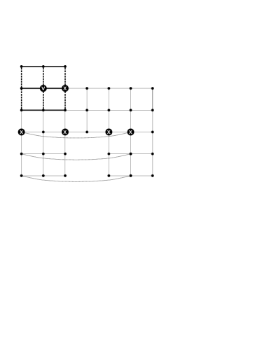
(a) A Cartesian prime graph $G=(V,E)$ is shown. For all vertices $x\in V$ (marked with ”X”) the respective $\mathfrak{d}_{|S_{x}}$ has only one equivalence class. Thus, we use only all non-”X”-marked vertices, pooled in the set $W\subseteq V$ and call Local $\mathfrak{d}_{|S_{v}}(W)^{*}$ computation (Alg. 1). The equivalence classes of $\mathfrak{d}_{|S_{v}}$ for vertex $v=v_{0}$ are highlighted by dashed and thick edges.

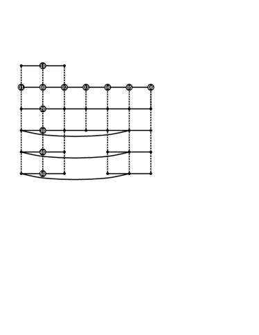
(b) After calling Local $\mathfrak{d}_{|S_{v}}(W)^{*}$ computation (Alg. 1) we obtain the equivalence classes of $\mathfrak{d}_{|S_{v}}(W)^{*}$ highlighted by dashed and thick edges. After calling Compute vertex coordinates (Alg. 2, Line 15 - 21) we obtain a graph where the vertices in each $G_{i}^{v}$-layer obtain unique coordinates.

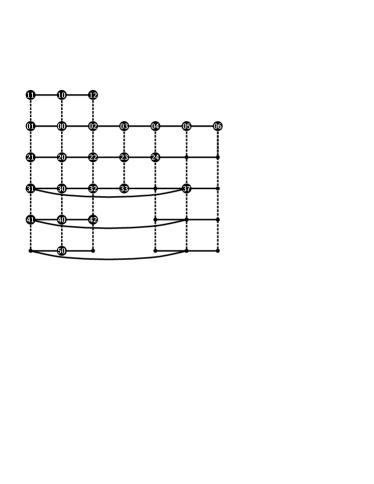
(c) Shown is the graph $G$ with coordinatized vertices for all $x\in\cup_{i=1}^{4}L_{i}$. Note, the vertex $x$ with coordinates $(37)$ obtained a new unused second coordinate $7$, since all edges $(u,x)$ where $u$ already obtained coordinates are from the same equivalence class (Alg. 2, Line 26). Thus, coordinates cannot be combined.

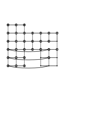
(d) Shown is the graph $G$ with coordinatized vertices for all $x\in\cup_{i=1}^{5}L_{i}$. Note, after running ConsistencyCheck (Alg. 3, Line 11) the edge between the vertices with coordinates $(37)$ and $(25)$ is deleted, since the vertices differ in more than one coordinate.

             

Figure 5. The basic steps of Algorithm 1 and 2

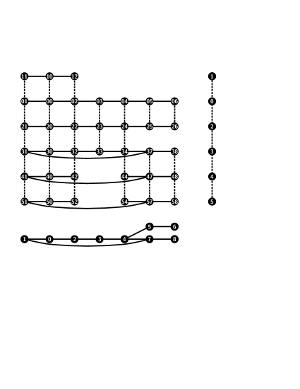
Figure 6. After running Algorithm 1 and 2 we obtain $H$ as a subgraph of the graph $G$ in Figure 5, with coordinatized vertices, and edges colored w.r.t. $\mathfrak{d}_{|S_{v}}(W)^{*}$ equivalence classes. After running Embedding of $H$ into Cartesian product (Alg. 4) we obtain the putative factors $H_{1}$ and $H_{2}$ of $H$ and, hence, of $G$. Note, due to the coordinatization of $H$ the embedding of $H$ into $H_{1}\Box H_{2}$ can easily be determined.

Lemma 4.4.

Given a graph $G=(V,E)$ with maximum degree $\Delta$ obtained from Algorithm 2 with coordinatized vertices. Then Algorithm 4 computes factors $H_{i}$ such that $G$ can be embedded into $\Box_{i=1}^{r}H_{i}$ in $O(|E|\Delta)$ time.

Proof.

After running Algorithm 2 we obtain a graph $G=(V,E)$ such that vertices $x\in V$ have consistent coordinates $c(x)=(c_{1}(x),\dots,c_{r}(x))$, i.e, no two vertices of $G$ have identical coordinates and adjacent vertices $x$ and $y$ with $(x,y)\in\varphi_{i}$ differ only in the $i$-th position of their coordinates.

We first compute empty graphs $H_{1},\dots,H_{r}$ and add for each vertex $x$ and for each $c_{i}(x)$ of its coordinates $c(x)=(c_{1}(x),\dots c_{r}(x))$ the vertex $c_{i}(x)$ to $H_{i}$. Different vertices $c_{i}(x)$ and $c_{i}(y)$ are connected in $H_{i}$ whenever there is an edge $(x,y)\in E$. We define a map $\gamma:V(G)\rightarrow V(H)$ with $x\mapsto c(x)$. Since no two vertices of $G$ have identical coordinates $\gamma$ is injective. Furthermore, since adjacent vertices $x$ and $y$ that differ only in one, say the $i$-th, position of their coordinates are mapped to the edge $(c_{i}(x),c_{i}(y))$ contained in factor $H_{i}$ and by definition of the Cartesian product, we can conclude that the map $\gamma$ is a homomorphism and hence, an embedding of $G$ into $H$.

The first two for-loops run $|V|\Delta$ times, that is $O(|E|)$. The second two for-loops run $|E|\Delta$ times, hence we end in overall time complexity of $O(|E|\Delta)$. ∎

To complete the paper, we explain how the last algorithms, in particular, Algorithm 1, 2 and 4 can be used as suitable heuristics to find approximate products; see also Figures 5 and 6. Note, by Corollary 4.2 Algorithm 1 can be used to compute $\delta(G)^{*}$. However, most graphs are prime and $\delta(G)^{*}$ would consist only of one equivalence class. Thus we are interested in subsets of $\delta(G)^{*}$ which provide enough information of large factorizable or “into non-trivial Cartesian product embeddable” subgraphs. This can be achieved by ignoring regions $S_{v}$ where $\mathfrak{d}_{|S_{v}}$ has only one or less than a given threshold number of equivalence classes. Hence, only subsets $W\subseteq V$ where $\mathfrak{d}_{|S_{v}}(W)^{*}$ has a sufficiently large number of equivalence classes are of interest. For this, we would cover a graph by starting at some vertex $v\in V$, compute $S_{v}$ and $\mathfrak{d}_{|S_{v}}$, and check if $\mathfrak{d}_{|S_{v}}$ has the desired number of equivalence classes; see Figure 5(a). If not, we take another vertex $w\in V$ and repeat this procedure with $w$. If $\mathfrak{d}_{|S_{v}}$ has the desired number of equivalence classes we would take a neighbor $w$ of $v$, compute $S_{w}$ and $\mathfrak{d}_{|S_{w}}$ and check whether $(\mathfrak{d}_{|S_{w}}\cup\mathfrak{d}_{|S_{v}})^{*}$ has the desired number of equivalence classes. If so, then we continue with neighbors of $v$ and $w$ and to extend the regions that can be embedded into a Cartesian product. To find such regions one can easily adapt Algorithms 2 and 4.

Note, after running Algorithm 1 one could take out one of largest connected component of each equivalence class induced by edges with the respective “colors” to obtain putative factors; see Figure 5(b). However, even knowing putative factors does not yield information about which edges should be added or deleted to obtain a product graph. For this, coordinates are necessary. They can be computed by Algorithm 2 and used as input for Algorithm 4; see Figure 6.

Finally, even the most general methods for computing approximate strong products only compute a (partial) product coloring of the graphs $G$ under investigation. They yield putative factors, but no coordinatization [9]. However, Algorithm 4 can be adapted to find the coordinates of the so-called underlying approximate Cartesian skeleton of such graphs, and can thus be used to find an embedding of (the approximate strong product) $G$ into a non-trivial strong product graph.

References

- [1] F. Aurenhammer, J. Hagauer, and W. Imrich. Cartesian graph factorization at logarithmic cost per edge. Computational Complexity, 2:331–349, 1992.
- [2] N. Chiba and T. Nishizeki. Arboricity and subgraph listing algorithms. SIAM Journal on Computing, 14(1):210–223, 1985.
- [3] J. Feigenbaum. Product graphs: some algorithmic and combinatorial results. Technical Report STAN-CS-86-1121, Stanford University, Computer Science, 1986. PhD Thesis.
- [4] J. Feigenbaum and R. A. Haddad. On factorable extensions and subgraphs of prime graphs. SIAM J. Discrete Math., 2:197–218, 1989.
- [5] J. Feigenbaum, J. Hershberger, and A. A. Schäffer. A polynomial time algorithm for finding the prime factors of Cartesian-product graphs. Discr. Appl. Math., 12:123–138, 1985.
- [6] R.L. Graham and P.M. Winkler. On isometric embeddings of graphs. Transactions of the American mathematical Society, 288(2):527–536, 1985.
- [7] J. Hagauer and J. Žerovnik. An algorithm for the weak reconstruction of Cartesian-product graphs. J. Combin. Inf. Syst. Sci., 24:97–103, 1999.
- [8] R. Hammack, W. Imrich, and S. Klavžar. Handbook of Product Graphs. Discrete Mathematics and its Applications. CRC Press, 2nd edition, 2011.
- [9] M. Hellmuth. A local prime factor decomposition algorithm. Discrete Mathematics, 311(12):944–965, 2011.
- [10] M. Hellmuth, W. Imrich, W. Klöckl, and P. F. Stadler. Approximate graph products. European J. Combin., 30:1119 – 1133, 2009.
- [11] M. Hellmuth, W. Imrich, W. Klöckl, and P. F. Stadler. Local algorithms for the prime factorization of strong product graphs. Math. Comput. Sci, 2(4):653–682, 2009.
- [12] M. Hellmuth, L. Ostermeier, and P. F. Stadler. Unique square property, equitable partitions, and product-like graphs. Discrete Mathematics, 2013. submitted, http://arxiv.org/abs/1301.6898.
- [13] W. Imrich and S Klavžar. Product graphs. Wiley-Interscience Series in Discrete Mathematics and Optimization. Wiley-Interscience, New York, 2000.
- [14] W. Imrich, S. Klavžar, and F. D. Rall. Topics in Graph Theory: Graphs and Their Cartesian Product. AK Peters, Ltd., Wellesley, MA, 2008.
- [15] W. Imrich and I. Peterin. Recognizing Cartesian products in linear time. Discrete Mathematics, 307(3 – 5):472 – 483, 2007.
- [16] W. Imrich, T. Pisanski, and J. Žerovnik. Recognizing Cartesian graph bundles. Discr. Math, 167-168:393–403, 1997.
- [17] W. Imrich and J. Žerovnik. On the weak reconstruction of Cartesian-product graphs. Discrete Math., 150(1-3):167–178, 1996.
- [18] W. Imrich and J. Žerovnik. Factoring Cartesian-product graphs. J. Graph Theory, 18:557–567, 1994.
- [19] W. Imrich, B. Zmazek, and J. Žerovnik. Weak k-reconstruction of Cartesian product graphs. Electronic Notes in Discrete Mathematics, 10:297 – 300, 2001. Comb01, Euroconference on Combinatorics, Graph Theory and Applications.
- [20] G. Sabidussi. Graph multiplication. Math. Z., 72:446–457, 1960.
- [21] J. Žerovnik. On recognition of strong graph bundles. Math. Slovaca, 50:289–301, 2000.
- [22] B. Zmazek and J. Žerovnik. Algorithm for recognizing Cartesian graph bundles. Discrete Appl. Math., 120:275–302, 2002.
- [23] B. Zmazek and J. Žerovnik. Weak reconstruction of strong product graphs. Discrete Math., 307:641–649, 2007.