Magnetization relaxation and geometric forces in a Bose ferromagnet

Abstract

We construct the hydrodynamic theory for spin-1/2 Bose gases at arbitrary temperatures. This theory describes the coupling between the magnetization, and the normal and superfluid components of the gas. In particular, our theory contains the geometric forces on the particles that arise from their spin’s adiabatic following of the magnetization texture. The phenomenological parameters of the hydrodynamic theory are calculated in the Bogoliubov approximation and using the Boltzmann equation in the relaxation-time approximation. We consider the topological Hall effect due to the presence of a skyrmion, and show that this effect manifests itself in the collective modes of the system. The dissipative coupling between the magnetization and the normal component is shown to give rise to magnetization relaxation that is fourth order in spatial gradients of the magnetization direction.

Introduction.— Geometric forces are abundant in virtually all areas of physics, from the classical conical pendulum Sakurai (1994) to a single quantum spin Zhang and Wu (2006). In particular after the advent of the Berry phase Berry (1984), a large number of manifestations of geometric forces, including the optical Magnus effect Bliokh et al. (2008), the topological Hall effect Neubauer et al. (2009); Li et al. (2013) and geometric forces due to synthetic gauge fields Dalibard et al. (2011) have been predicted and observed.

In metallic ferromagnets, magnetization dynamics leads to forces on quasiparticles of geometric origin called spin motive forces, that have gained considerable attention recently Barnes and Maekawa (2007); Duine (2008); Tserkovnyak and Wong (2009); Yang et al. (2009); Hayashi et al. (2012). Furthermore, spin textures with nonzero chirality, such as the skyrmion lattice observed recently Mühlbauer et al. (2009); Yu et al. (2011) induce the so-called topological Hall effect Neubauer et al. (2009); Li et al. (2013). In addition, the coupling between magnetization and quasiparticles has also been shown to give rise to novel forms of magnetization relaxation in this case. A prominent example is inhomogeneous Gilbert damping Foros et al. (2008); Zhang and Zhang (2009); Gómez et al. (2010). This effect is important in clean solid-state systems. We therefore expect these effects to be particularly important for gases of ultracold atoms, that, in contrast to conventional condensed-matter systems, are free of impurities.

The field of ultracold atoms is characterised by exquisite experimental control Anderson et al. (1995); Davis et al. (1995); Chin et al. (2010). Relevant for our focus is the great amount of recent activity on spinor Bose gases. Firstly, it has been discovered that these gases can be either ferromagnetic or antiferromagnetic depending on the details of the scattering lengths Ho (1998); Ohmi and Machida (1998). Furthermore, numerous studies at zero temperature, based on the Gross-Pitaevskii equation, have elucidated the long-wavelength properties of spinor gases Lamacraft (2008); Barnett et al. (2009). Other areas of current interest in the field include topological excitations, magnetic dipole-dipole interactions and non-equilibrium quantum dynamics Kawaguchi and Ueda (2012). The recent progress in the understanding of ferromagnetic spinor gases and their manipulation by light has also enabled detailed studies of magnetization dynamics Sadler et al. (2006); Stamper-Kurn and Ueda (2012).

Despite these activities, a theory that describes simultaneously all phases of ferromagnetic spinor Bose gases and includes both geometric and dissipative coupling between superfluid, ferromagnetic order parameter and quasiparticles is lacking. The purpose of this Letter is to put forward such a theory. This theory is needed to determine properties of collective modes at arbitrary temperatures that consist of combined dynamics of the ferromagnetic and superfluid order with the normal component of the gas. These results can e.g. be used to detect the presence of skyrmions and their dynamics in the gas. We choose to work in the hydrodynamic regime, where the coupling between the magnetization, and the normal and superfluid components of the gas is controlled by a gradient expansion. This approach is valid in the regime where local equilibrium is enforced by frequent collisions. In addition, we make a connection between long-wavelength and microscopic physics by calculating all the hydrodynamic parameters from first principles. In the microscopic determination of the parameters, we focus on the spin-1/2 case leaving higher spin for future work.

Hydrodynamic equations.— Describing a ferromagnetic Bose gas requires considering three phases: unpolarized normal fluid, normal ferromagnet and superfluid ferromagnet. These three phases have different sets of relevant hydrodynamic variables, that have to be taken into account in order to fully describe the behavior of the system. A complete set of relevant variables includes the order parameters and the conserved quantities. The order parameters of a homogeneous Bose ferromagnet are the superfluid velocity $\boldsymbol{v}_{s}$ and the magnetization density $Pn\Omega^{\alpha}$. Here $P$ is the polarization, and $\Omega^{\alpha}$ is the dimensionless magnetization direction, normalized such that $\Omega^{\alpha}\Omega^{\alpha}=1$. (We use the Einstein summation convention throughout the paper.) The conserved quantities are the total particle density $n$, the total particle current $\boldsymbol{j}$, the magnetization density $Pn\Omega^{\alpha}$ and the energy. In the hydrodynamic approach we write for each conserved quantity a continuity equation. Not considering energy conservation for simplicity, we therefore have the following set of hydrodynamic equations:

$$\partial_{t}n+\boldsymbol{\nabla}\cdot\boldsymbol{j}=0,$$ (1)

$$\partial_{t}\left(Pn\Omega^{\alpha}\right)+{\boldsymbol{\nabla}}\cdot\left((\boldsymbol{j}_{\mathrm{spin}}^{\perp})^{\alpha}+(\boldsymbol{j}_{\mathrm{spin}}^{\parallel})^{\alpha}\right)=0,$$ (2)

$$m\partial_{t}\boldsymbol{j}+m\boldsymbol{\nabla}\cdot\boldsymbol{\Pi}+n\boldsymbol{\nabla}V-Pn\boldsymbol{E}-P\boldsymbol{j}\times\boldsymbol{B}=0.$$ (3)

In these equations, $m$ is the particle mass, $\boldsymbol{\Pi}=n_{n}\boldsymbol{v}_{n}\boldsymbol{v}_{n}+n_{s}\boldsymbol{v}_{s}\boldsymbol{v}_{s}+\boldsymbol{1}\,p/m$ is the energy-momentum tensor, and $V$ is the trapping potential. We have also introduced the pressure $p$, the normal fluid velocity $\boldsymbol{v}_{n}$ and the normal fluid density $n_{n}$, and equivalent quantities $\boldsymbol{v}_{s}$ and $n_{s}$ for the superfluid. We use these quantities to define the normal and superfluid particle currents $\boldsymbol{j}_{n}=n_{n}\boldsymbol{v}_{n}$ and $\boldsymbol{j}_{s}=n_{s}\boldsymbol{v}_{s}$, such that $\boldsymbol{j}=\boldsymbol{j}_{n}+\boldsymbol{j}_{s}$. The total density is then $n=n_{s}+n_{n}$. Note that coordinate space tensors and vectors are denoted by bold font, while spin space vector components are denoted by Greek superscripts.

The coupling between magnetization and normal fluid leads to geometric forces Volovik (1987); Stern (1992). These can e.g. be understood as resulting from the Berry curvature and spin Berry phases that the atoms pick up as their spin adiabatically follows the magnetization texture. More concretely, there exist now an artificial electric field

$$\boldsymbol{E}=\hbar\varepsilon^{\alpha\beta\gamma}\Omega^{\alpha}(\partial_{t}\Omega^{\beta})(\boldsymbol{\nabla}\Omega^{\gamma})/2$$ (4)

and an artificial magnetic field

$$\boldsymbol{B}=-\hbar\varepsilon^{\alpha\beta\gamma}\Omega^{\alpha}(\boldsymbol{\nabla}\Omega^{\beta})\times(\boldsymbol{\nabla}\Omega^{\gamma})/4,$$ (5)

where we have introduced the totally antisymmetric Levi-Civita tensor $\varepsilon^{\alpha\beta\gamma}$. As we have already seen in Eq. (3), these fields enter the hydrodynamic equations as the electric and magnetic parts of the Lorentz force, respectively, acting on the particle current.

A more detailed discussion on the spin currents is now in order. The longitudinal spin current describes spin transport with spin polarization along the magnetization direction due to particle currents: $(\boldsymbol{j}_{\mathrm{spin}}^{\parallel})^{\alpha}=P\boldsymbol{j}\Omega^{\alpha}$. The transverse spin current has, to lowest order in the gradient expansion, terms proportional to the spin stiffness $A_{\mathrm{s}}$ and a parameter proportional to the transverse spin diffusion constant $\eta_{\perp}$ Tserkovnyak et al. (2009):

$$(\boldsymbol{j}_{\mathrm{spin}}^{\perp})^{\alpha}=-\varepsilon^{\alpha\beta\gamma}\frac{1}{n}\eta_{\perp}\Omega^{\beta}(n\partial_{t} +\boldsymbol{j}\cdot\boldsymbol{\nabla})\boldsymbol{\nabla}\Omega^{\gamma}\qquad\qquad$$

$$-A_{s}\varepsilon^{\alpha\beta\gamma}\Omega^{\beta}\boldsymbol{\nabla}\Omega^{\gamma}.$$ (6)

The first term describes transverse spin relaxation. It contains the usual hydrodynamic derivative and illustrates the fact that only gradients of magnetization relax because spin is conserved in our system. The second term represents non-dissipative transverse spin transport. Note that the above results can be understood as containing all symmetry-allowed terms up to second order in gradients. The superfluid velocity obeys the Josephson relation

$$m\partial_{t}\boldsymbol{v}_{s}+\boldsymbol{\nabla}\left[mv_{s}^{2}/2+V+\mu\right]-\boldsymbol{E}=0,$$ (7)

where $\mu$ is the chemical potential, and also the Mermin-Ho relation

$$m\boldsymbol{\nabla}\times\boldsymbol{v}_{s}=-\boldsymbol{B}.$$ (8)

This completes the set of hydrodynamic equations.

Our hydrodynamic equations correctly describe the system at any temperature relevant for cold-atom experiments. At sufficiently low temperatures both order parameters are non-zero, and we have a ferromagnetic Bose-Einstein condensate with a negligible normal fluid density. Setting the normal fluid density and its velocity to zero, and setting the polarization to $P=1$, we obtain the well-known $T=0$ limit Kawaguchi and Ueda (2012). At higher temperatures, where the normal fluid density is sizable, we have to use the full set of equations. Heating the system even further results in the disappearance of the Bose-Einstein condensate at $T_{\text{BEC}}$. (Note that in general the critical temperature for Bose-Einstein condensation is lower than the ferromagnetic transition temperature, as shown in Ref. Gu et al. (2004).) We then have to discard Eqs. (7) and (8), and set the superfluid density as well as its velocity to zero. Finally, in the high temperature limit $T>T_{\text{FM}}$, the average magnetization is zero, and the distinction between longitudinal and transverse spin polarization disappears. In addition, there are no artificial electromagnetic fields and consequently the geometric forces vanish. For those reasons, the spin current becomes $\boldsymbol{j}_{\mathrm{spin}}^{\alpha}=-D_{s}\boldsymbol{\nabla}(n\Omega^{\alpha})$, where $D_{s}$ is the spin diffusion constant, which is related to the longitudinal spin relaxation time determined previouslyDuine and Stoof (2009).

Collective modes.— As a first application of the above, we consider the collective modes. Following the usual procedure, we linearize the equations and put in a plane-wave ansatz for the hydrodynamical variables. Solving for frequency $\omega$ as a function of momentum $k$ results in

$$\omega=k\sqrt{\frac{1}{m}\frac{\partial p}{\partial n}}\equiv ck,$$ (9)

$$\omega=\frac{A_{s}(Pnk^{2}-i\eta_{\perp}k^{4})}{\eta_{\perp}^{2}k^{4}+(Pn)^{2}}\overset{k\rightarrow 0}{\longrightarrow}\frac{A_{s}}{Pn}k^{2}-\frac{i\eta_{\perp}A_{s}}{(Pn)^{2}}k^{4}.$$ (10)

The first equation describes a density wave, first sound, which propagates at the speed of sound $c$ as expected. The second equation gives the dispersion for the spin waves and includes their damping. We remark that in the long-wavelength limit it reduces to a quadratic dispersion with quartic damping, which is in agreement with previous results for conventional (Fermi) ferromagnets Halperin and Hohenberg (1969). Finally, we did not consider energy as a hydrodynamic variable and hence neglected the resulting heat diffusion. Thus, our theory does not properly predict the velocity of second sound.

Skyrmion dynamics and topological Hall effect.— To illustrate the importance of geometrical forces, we investigate the motion of a 2D or baby skyrmion (Fig. 1). There are several reasons warranting a closer look at this 2D skyrmion. Firstly, we expect to see a topological Hall effect, due to the artificial electromagnetic fields generated by the spin texture. Moreover, due to the interplay between magnetization relaxation and spin gradients, we anticipate irreversible dynamics. Lastly, baby skyrmions have been experimentally realized in spinor Bose gases Choi et al. (2012), suggesting that our theory could be confronted with experiments in the near future.

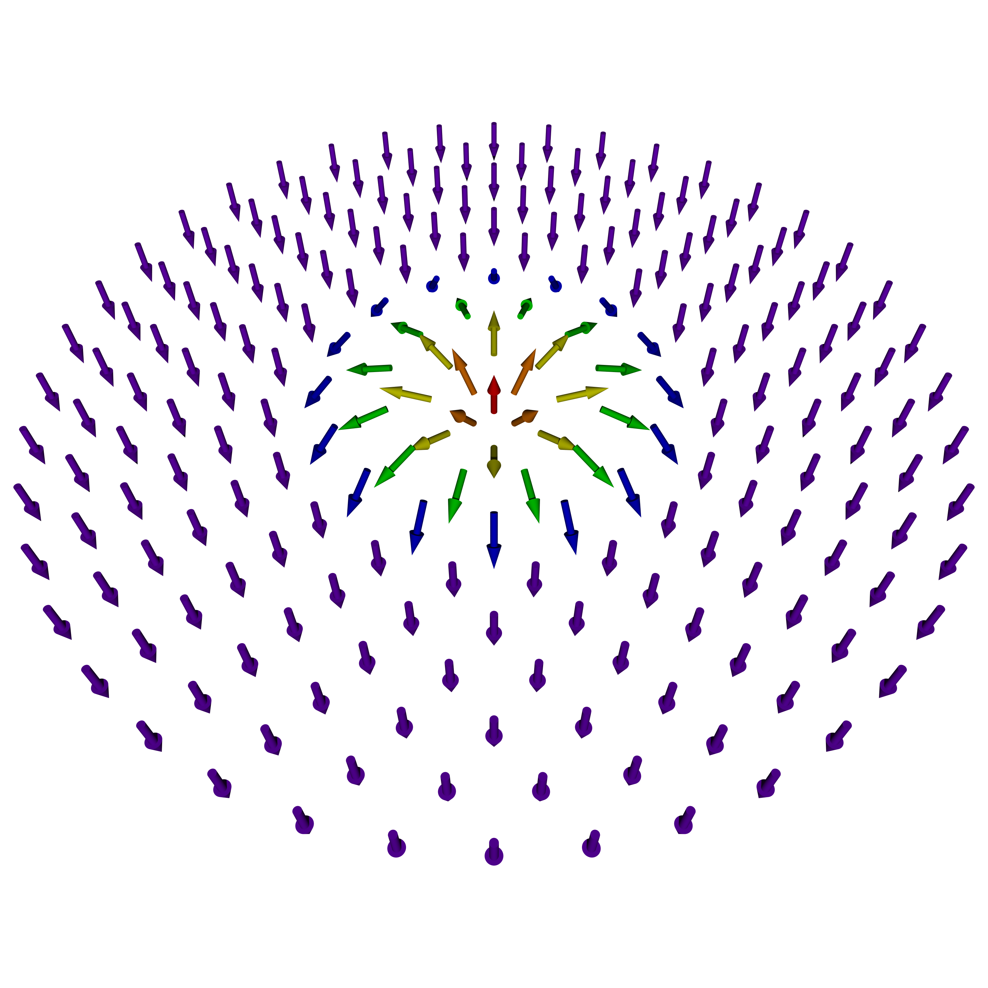
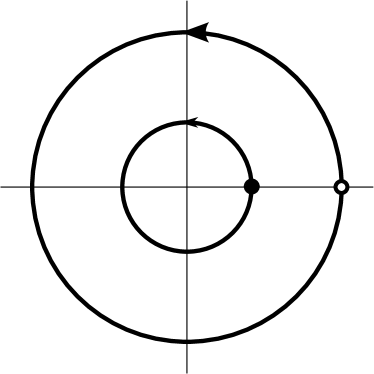
Figure 1: A baby skyrmion in a two-dimensional ferromagnetic cloud (left). In an isotropic trap, which has its center in the middle of the picture (right), the skyrmion (empty circle) precesses around the center of the trap. The center of the cloud (filled circle) also moves around the center of the trap due to the topological Hall effect. The amplitude of the motion of the center of the cloud has been enhanced for clarity.

Considering a rigid skyrmion texture $\Omega^{\alpha}=\Omega^{\alpha}(\boldsymbol{x}-\boldsymbol{x}_{\text{sk}})$ with a velocity $\boldsymbol{v}_{\text{sk}}=(\dot{x}_{\text{sk}},\dot{y}_{\text{sk}})$, we derive its equations of motion from our hydrodynamic description of the dynamics of the atomic cloud. To that end, we take a cross product of $\Omega^{\alpha}$ with Eq. (2), then take an inner product with $\boldsymbol{\nabla}\Omega^{\alpha}$ and finally perform an integral over the coordinate space. Moreover, we assume a pancake-like geometry at a low temperature, and a Thomas-Fermi density profile for this calculation. We define the trap to be isotropic and harmonic in the $xy$-plane with the frequency $\omega_{d}$. Furthermore, $\eta_{\perp}$ is taken to be constant, $A_{s}(\boldsymbol{x})=n(\boldsymbol{x})a_{s}$, and $a_{s}=\hbar P/2m$ as is shown below. We also introduce the density in the center of the cloud $n_{0}$, the density in the center of the skyrmion $n_{\text{sk}}$ and the radius of the cloud $R$. The equations of motion ultimately read

$$\ddot{x}+\omega_{d}^{2}x-\Delta\dot{y}P\hbar I^{1}_{12}n_{\text{sk}}/\pi mn_{0}R^{2}=0,$$

$$\ddot{y}+\omega_{d}^{2}y+\Delta\dot{x}P\hbar I^{1}_{12}n_{\text{sk}}/\pi mn_{0}R^{2}=0,$$

$$\Delta\dot{x}(\eta_{\perp}I^{2}_{12}+n_{\text{sk}}PI_{12}^{1})+\Delta\dot{y}\eta_{\perp}I^{2}_{22}+\Delta yn_{0}a_{s}I^{3}/R^{2}=0,$$

$$\Delta\dot{y}(\eta_{\perp}I^{2}_{12}-n_{\text{sk}}PI_{12}^{1})+\Delta\dot{x}\eta_{\perp}I^{2}_{11}+\Delta xn_{0}a_{s}I^{3}/R^{2}=0,$$

where $\Delta x=x_{\text{sk}}-x$ and $\Delta y=y_{\text{sk}}-y$ are the skyrmion coordinates relative to the center of the cloud. The quantities $I^{1}_{ij}$, $I^{2}_{ij}$ and $I^{3}$ are real and only depend on the texture int , where $i$, $j$ can be $1$ or $2$, corresponding to the $x$ or $y$ direction, respectively. The integral $I^{1}_{12}$ is determined by a topological invariant known as the skyrmion number or the winding number: $W=I^{1}_{12}/4\pi=1$. Furthermore, for cylindrically symmetric skyrmion textures, $I^{3}=h$ and $I^{2}_{ij}=-\tilde{h}\delta_{ij}/l^{2}$, where $h$ and $\tilde{h}$ are dimensionless numbers, while $l$ is the length associated with the size of the skyrmion con . The latter integrals are therefore not determined by the topology of the magnetization texture only.

Following the procedure described above, we find, in addition to the dipole mode with frequency $\omega_{d}$, a collective mode pertaining to the motion of the skyrmion with the frequency

$$\omega_{\text{sk}}=\frac{hn_{0}\hbar\left(4n_{\text{sk}}P\pi+i\tilde{h}\eta_{\perp}/l^{2}\right)}{2mR^{2}\left(16n_{\text{sk}}^{2}P^{2}\pi^{2}+\tilde{h}^{2}\eta_{\perp}^{2}/l^{4}\right)}.$$ (11)

The real part of the frequency implies that the skyrmion is moving around the center of the trap, c.f. Fig. 1, while the positive imaginary part means that the skyrmion is spiraling out and is pushed away from the center of the trap.

We now turn our attention to the case of no damping ($\eta_{\perp}=0$). The eigenvectors of the various modes, written in the form $(x,y,\Delta x,\Delta y)$, are $(1,0,0,0)$, $(0,1,0,0)$, $(-i\alpha,\alpha,-i,1)$ and $(i\alpha,\alpha,i,1)$ with

$$\alpha=\frac{32hn_{\text{sk}}^{2}P^{2}\pi\hbar^{2}}{64m^{2}n_{\text{sk}}^{2}P^{2}\pi^{2}R^{4}\omega_{d}^{2}-h^{2}n_{0}^{2}\hbar^{2}}.$$ (12)

The first two eigenvectors describe the dipole mode, where the cloud and the skyrmion move in phase in either the $x$ or the $y$ direction, respectively. In order to investigate the implications of the third and fourth eigenvectors, we set the initial coordinates $\Delta x(0)\neq 0$ and $x(0)=\alpha\Delta x(0)$ with $y(0)=\Delta y(0)=0$. We set the initial velocity of the cloud to zero. In that case, $x$ and $\Delta x$ oscillate in phase with the frequency $\omega_{\text{sk}}=hn_{0}\hbar/8mn_{\text{sk}}P\pi R^{2}$:

$$x=\alpha\Delta x(0)\cos(\omega_{\text{sk}}t),\quad\Delta x =\Delta x(0)\cos(\omega_{\text{sk}}t).$$ (13)

However, both the center of the cloud and the skyrmion start moving in the $y$ direction is as well (cf. Fig. 1):

$$y =\alpha\Delta x(0)\left[\sin(\omega_{\text{sk}}t)-\frac{\omega_{\text{sk}}}{\omega_{d}}\sin(\omega_{d}t)\right],$$ (14)

$$\Delta y =\Delta x(0)\sin(\omega_{\text{sk}}t),$$ (15)

due to the force exerted on them by the artificial electromagnetic field, which can also be seen in the equations of motion. Physically, this effect is a Hall effect as it corresponds to transverse motion in response to a longitudinal force – in this case the restoring force of the trapping potential. Due to the nature of this particular spin texture, this effect is known as the topological Hall effect.

Microscopic theory.— We proceed to evaluate the hydrodynamic input parameters $P$, $A_{s}$ and $\eta_{\perp}$. To calculate the polarization $P$, we employ the Bogoliubov theory around the ferromagnetic groundstate of the gas. That amounts to populating only one of the condensate components, $n_{c}^{\uparrow}=n_{c}\neq 0$, while $n_{c}^{\downarrow}=0$. Scattering amplitudes in ultracold gases are governed by the two-body T matrix $g$ Stoof et al. (2009), which can have different components for collisions of different spin states. We only consider the case with equal T-matrix elements $g^{\uparrow\downarrow}=g^{\uparrow\uparrow}=g^{\downarrow\downarrow}=g\neq 0$. Furthermore, we investigate a balanced mixture, i.e., with equal chemical potentials $\mu^{\uparrow}=\mu^{\downarrow}=gn_{c}^{\uparrow}$. This leads to decoupling of the spin components. The $\uparrow$ particles obtain the usual Bogoliubov propagator, while the $\downarrow$ particles retain the non-interacting propagator within this approximation. We thus find the following particle densities in the non-condensate states:

$$n^{\uparrow}_{\mathrm{nc}}=\frac{1}{V}\sum_{\boldsymbol{k}\neq 0}\left(\frac{\varepsilon_{k}+gn_{c}}{\hbar\omega_{k}}\right. \frac{1}{e^{\beta\hbar\omega_{k}}-1}$$

$$+\left.\frac{\varepsilon_{k}+gn_{c}-\hbar\omega_{k}}{2\hbar\omega_{k}}\right),$$ (16)

and $n^{\downarrow}_{nc}=\sum_{\boldsymbol{k}\neq 0}[\exp({\beta\varepsilon_{k}})-1]^{-1}/V,$ where the Bogoliubov dispersion $\hbar\omega_{k}=\sqrt{\varepsilon_{k}(\varepsilon_{k}+2gn_{c})}$, $\beta=1/k_{\mathrm{B}}T$ is the inverse thermal energy and $\varepsilon_{k}=\hbar^{2}k^{2}/2m$ is the free particle dispersion. The density distributions are subject to the constraint $n=n_{c}+n^{\uparrow}_{nc}+n^{\downarrow}_{nc}$. We note that after fixing the total density $n$, temperature and interaction strength, we can solve these equations for $n_{c}$ and obtain $n_{nc}^{\uparrow}$ as well as $n_{nc}^{\downarrow}$ at the same time. This gives us the polarization of the gas

$$P=(n_{c}+n^{\uparrow}_{nc}-n^{\downarrow}_{nc})/n=1-2n^{\downarrow}_{nc}/n.$$ (17)

In the intermediate temperature regime $ng\ll k_{B}T<k_{B}T_{\text{BEC}}$ it is straightforward to calculate $P$ analytically. To that end, we approximate $\hbar\omega_{k}\simeq\varepsilon_{k}+gn_{c}$, so that $n_{nc}^{\uparrow}=n_{nc}^{\downarrow}=\zeta(3/2)(mk_{\mathrm{B}}T/2\pi\hbar^{2})^{3/2}$ and

$$P=1-2\zeta(3/2)(mk_{B}T/2\pi\hbar^{2})^{3/2}/n,$$ (18)

where $\zeta$ denotes the Riemann zeta function. Note that in this approximation we have $P=1$ at zero temperature, as the depletion of the condensate is neglected and all the ideal gas particles end up in the condensate.

We now turn to the calculation of the spin stiffness $A_{s}$. According to the Bogoliubov theory, when only one spin component is populated with a Bose-Einstein condensate, excitations in the other spin components are free particles, corresponding to spin waves. Therefore, the dispersion of the spin waves is simply $\hbar\omega_{k}=\varepsilon_{k}$. Comparing this with the real part of the dispersion relation for the spin waves given by the hydrodynamics in Eq. (10), we conclude that

$$A_{s}=\frac{\hbar}{2m}Pn.$$ (19)

The only quantity that remains to be evaluated is $\eta_{\perp}$. An upper bound for this quantity is found by considering the non-condensed phase. In this case, we note that it is equal to the transverse spin conductivity Tserkovnyak et al. (2009)

$$\eta_{\perp}=\hbar\sigma_{\perp}.$$ (20)

We calculate $\sigma_{\perp}$ in the normal phase from a set of Boltzmann equations and use the relaxation-time approximation. For a given species, e.g. $\uparrow$, the momentum-dependent relaxation time $(\tau^{\uparrow\uparrow})_{k}$ is given by the well-known collision integral

$$\frac{1}{(\tau^{\uparrow\uparrow})_{k}}= \frac{2\pi}{\hbar}g_{\uparrow\downarrow}^{2}\int\frac{\,\mathrm{d}\boldsymbol{k}_{2}}{(2\pi)^{3}}\frac{\,\mathrm{d}\boldsymbol{k}_{3}}{(2\pi)^{3}}\frac{\,\mathrm{d}\boldsymbol{k}_{4}}{(2\pi)^{3}}f^{\downarrow\downarrow}(\boldsymbol{k}_{2})[1+f^{\uparrow\uparrow}(\boldsymbol{k}_{3})]$$

$$\times[1+f^{\downarrow\downarrow}(\boldsymbol{k}_{4})](2\pi)^{3}\delta^{(3)}(\boldsymbol{k}+\boldsymbol{k}_{2}-\boldsymbol{k}_{3}-\boldsymbol{k}_{4})$$

$$\times\delta(\varepsilon_{k}+\varepsilon_{k_{2}}-\varepsilon_{k_{3}}-\varepsilon_{k_{4}}),$$ (21)

that can be derived using Fermi’s golden rule. Here we only consider the term due to inter-species scattering, as intra-species scattering terms drive the distributions $f^{\uparrow\uparrow}$ and $f^{\downarrow\downarrow}$ towards the Bose-Einstein equilibrium distribution.

The transverse spin relaxation time is then given by

$$2/(\tau^{\perp}_{s})_{k}=1/(\tau^{\uparrow\uparrow})_{k}+1/(\tau^{\downarrow\downarrow})_{k}.$$ (22)

Given this relaxation time, the transverse spin conductivity is obtained by evaluating the integral

$$\eta_{\perp}=-\frac{\hbar^{3}}{m^{2}}\int\,\mathrm{d}\boldsymbol{k}k^{2}\frac{(\tau_{s}^{\perp})_{k}}{1+[(\tau_{s}^{\perp})_{k}\Delta/\hbar]^{2}}\frac{\partial f_{0}}{\partial\varepsilon_{k}},$$ (23)

where $f_{0}$ is the sum of the equilibrium distributions of $\uparrow$ and $\downarrow$ particles and $\Delta=\mu^{\uparrow}-\mu^{\downarrow}$ is the exchange splitting. For a particular kind of atom, $\eta_{\perp}$ depends on the temperature and all the scattering lengths in the system. However, by fixing the inter-species T matrix $g_{\uparrow\downarrow}$, we can obtain a more general picture as a function of temperature and polarization as shown in Fig. 2.

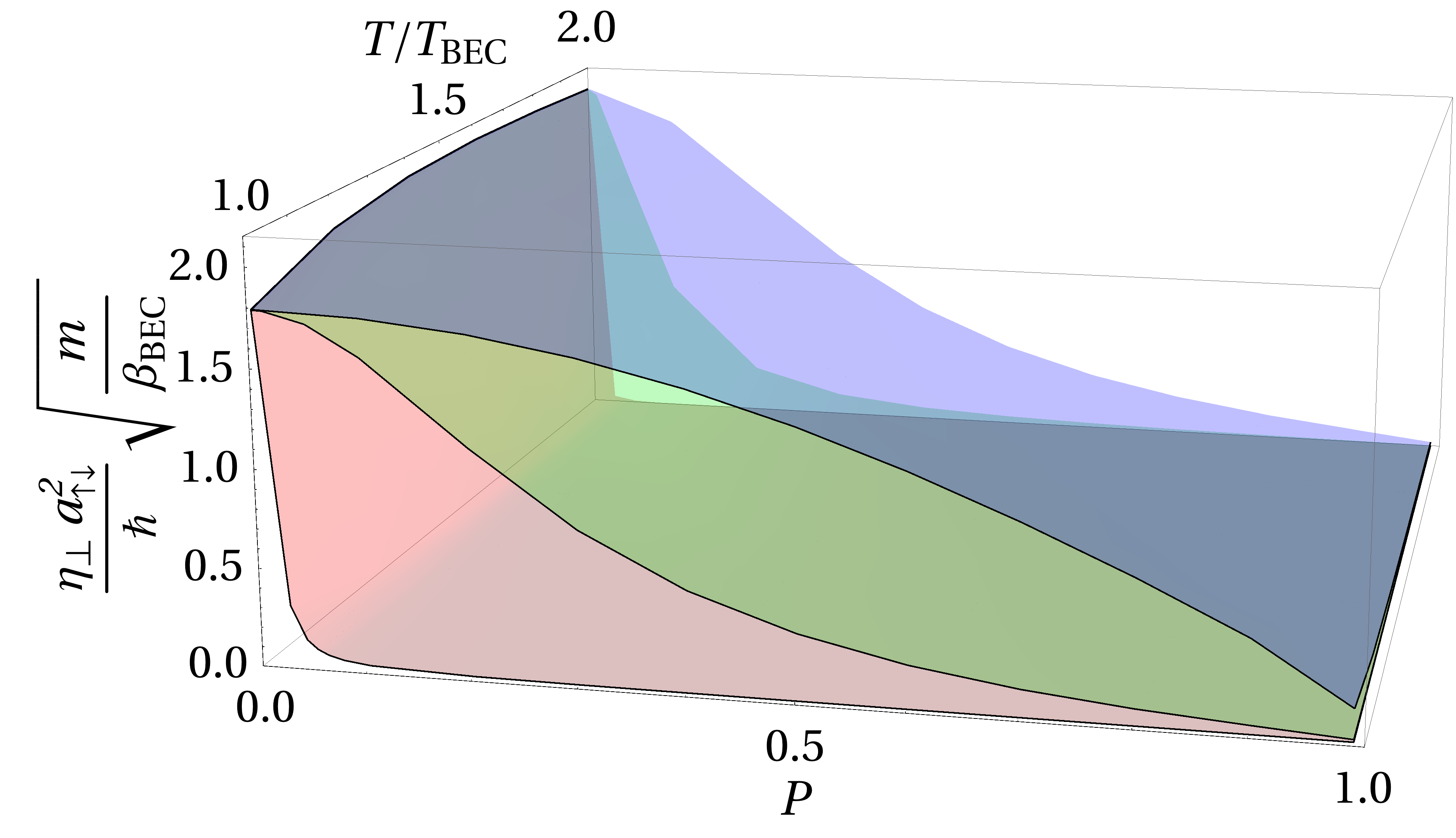
Figure 2: Transverse spin diffusion $\eta_{\perp}$ as a function of polarization $P$ and temperature for a homogeneous gas. The three surfaces correspond to $ng_{\uparrow\downarrow}\beta_{\text{BEC}}=1$, $0.5$ and $0.1$ from top to bottom. Here $a_{\uparrow\downarrow}$ is the inter-species scattering length and $\beta_{\text{BEC}}\equiv 1/k_{B}T_{\text{BEC}}$.

Discussion and conclusion.— In summary, we have constructed a hydrodynamic theory for a ferromagnetic spin-1/2 Bose gas that is valid for any temperature relevant for cold-atom systems. We have also calculated all the input parameters for the hydrodynamic theory within the Bogoliubov approximation. Finally, we have considered dynamics of a topological spin texture (skyrmion) and found it to lead to a topological Hall effect.

To determine if the topological Hall effect can be observed experimentally, we estimate the skyrmion precession frequency $\omega_{\text{sk}}$ and the eigenvector parameter $\alpha$. Considering a condensate of $10^{4}$ ²³Na atoms in a pancake-like geometry with radial confinement $\omega_{\perp}/2\pi=1\,\text{Hz}$ and perpendicular confinement $\omega_{z}=10\omega_{\perp}$, we estimate $\omega_{\text{sk}}=\omega_{\perp}$ and $\alpha=0.1$. This corresponds to a cloud size of $50\,\mu m$ and a Hall amplitude of $5\,\mu m$, which should be observable with current experimental techniques.

When it comes to the damping of spin waves, we consider a homogeneous ⁸⁷Rb gas ($|F=1,m_{f}=-1\rangle$ and $|F=2,m_{f}=1\rangle$) with the density of $10^{16}$ cm^-3 as an example. In particular, at the Bose-Einstein condensation temperature and polarization $P=1/2$ a spin wave with momentum $k=1\,\mu m^{-1}$, which is within the reach of current experiments, has a damping time of $0.7$ s.

In the future work, we plan to calculate $\eta_{\perp}$ in the superfluid phase ($T<T_{\text{BEC}}$), which would complete the microscopic input for the parameters of the hydrodynamic theory in the entire temperature range. Moreover, it is worthwhile to apply the current approach to higher spin systems, where extra degrees of freedom such as the nematic tensor Yukawa and Ueda (2012) enter the theory.

This work is supported by the Stichting voor Fundamenteel Onderzoek der Materie (FOM) and the Nederlandse Organisatie voor Wetenschaplijk Onderzoek (NWO).

References

- Sakurai (1994) J. J. Sakurai, Modern Quantum Mechanics, Revised ed. (Addison-Wesley Publishing Company, Reading, 1994).
- Zhang and Wu (2006) Q. Zhang and B. Wu, Phys. Rev. Lett. 97, 190401 (2006).
- Berry (1984) M. V. Berry, Proceedings of the Royal Society of London. A. Mathematical and Physical Sciences 392, 45 (1984).
- Bliokh et al. (2008) K. Y. Bliokh, A. Niv, V. Kleiner, and E. Hasman, Nat Photon 2, 748 (2008).
- Neubauer et al. (2009) A. Neubauer, C. Pfleiderer, B. Binz, A. Rosch, R. Ritz, P. G. Niklowitz, and P. Böni, Phys. Rev. Lett. 102, 186602 (2009).
- Li et al. (2013) Y. Li, N. Kanazawa, X. Z. Yu, A. Tsukazaki, M. Kawasaki, M. Ichikawa, X. F. Jin, F. Kagawa, and Y. Tokura, Phys. Rev. Lett. 110, 117202 (2013).
- Dalibard et al. (2011) J. Dalibard, F. Gerbier, G. Juzeliūnas, and P. Öhberg, Rev. Mod. Phys. 83, 1523 (2011).
- Barnes and Maekawa (2007) S. E. Barnes and S. Maekawa, Phys. Rev. Lett. 98, 246601 (2007).
- Duine (2008) R. A. Duine, Phys. Rev. B 77, 014409 (2008).
- Tserkovnyak and Wong (2009) Y. Tserkovnyak and C. H. Wong, Phys. Rev. B 79, 014402 (2009).
- Yang et al. (2009) S. A. Yang, G. S. D. Beach, C. Knutson, D. Xiao, Q. Niu, M. Tsoi, and J. L. Erskine, Phys. Rev. Lett. 102, 067201 (2009).
- Hayashi et al. (2012) M. Hayashi, J. Ieda, Y. Yamane, J.-i. Ohe, Y. K. Takahashi, S. Mitani, and S. Maekawa, Phys. Rev. Lett. 108, 147202 (2012).
- Mühlbauer et al. (2009) S. Mühlbauer, B. Binz, F. Jonietz, C. Pfleiderer, A. Rosch, A. Neubauer, R. Georgii, and P. Böni, Science 323, 915 (2009).
- Yu et al. (2011) X. Z. Yu, N. Kanazawa, Y. Onose, K. Kimoto, W. Z. Zhang, S. Ishiwata, Y. Matsui, and Y. Tokura, Nat Mater 10, 106 (2011).
- Foros et al. (2008) J. Foros, A. Brataas, Y. Tserkovnyak, and G. E. W. Bauer, Phys. Rev. B 78, 140402 (2008).
- Zhang and Zhang (2009) S. Zhang and S. S.-L. Zhang, Phys. Rev. Lett. 102, 086601 (2009).
- Gómez et al. (2010) J. Gómez, F. Perez, E. M. Hankiewicz, B. Jusserand, G. Karczewski, and T. Wojtowicz, Phys. Rev. B 81, 100403 (2010).
- Anderson et al. (1995) M. H. Anderson, J. R. Ensher, M. R. Matthews, C. E. Wieman, and E. A. Cornell, Science 269, 198 (1995).
- Davis et al. (1995) K. B. Davis, M. O. Mewes, M. R. Andrews, N. J. van Druten, D. S. Durfee, D. M. Kurn, and W. Ketterle, Phys. Rev. Lett. 75, 3969 (1995).
- Chin et al. (2010) C. Chin, R. Grimm, P. Julienne, and E. Tiesinga, Rev. Mod. Phys. 82, 1225 (2010).
- Ho (1998) T.-L. Ho, Phys. Rev. Lett. 81, 742 (1998).
- Ohmi and Machida (1998) T. Ohmi and K. Machida, Journal of the Physical Society of Japan 67, 1822 (1998).
- Lamacraft (2008) A. Lamacraft, Phys. Rev. A 77, 063622 (2008).
- Barnett et al. (2009) R. Barnett, D. Podolsky, and G. Refael, Phys. Rev. B 80, 024420 (2009).
- Kawaguchi and Ueda (2012) Y. Kawaguchi and M. Ueda, Physics Reports 520, 253 (2012).
- Sadler et al. (2006) L. E. Sadler, J. M. Higbie, S. R. Leslie, M. Vengalattore, and D. M. Stamper-Kurn, Nature 443, 312 (2006).
- Stamper-Kurn and Ueda (2012) D. M. Stamper-Kurn and M. Ueda, ArXiv e-prints (2012), arXiv:1205.1888 .
- Volovik (1987) G. E. Volovik, Journal of Physics C: Solid State Physics 20, L83 (1987).
- Stern (1992) A. Stern, Phys. Rev. Lett. 68, 1022 (1992).
- Tserkovnyak et al. (2009) Y. Tserkovnyak, E. M. Hankiewicz, and G. Vignale, Phys. Rev. B 79, 094415 (2009).
- Gu et al. (2004) Q. Gu, K. Bongs, and K. Sengstock, Phys. Rev. A 70, 063609 (2004).
- Duine and Stoof (2009) R. A. Duine and H. T. C. Stoof, Phys. Rev. Lett. 103, 170401 (2009).
- Halperin and Hohenberg (1969) B. I. Halperin and P. C. Hohenberg, Phys. Rev. 188, 898 (1969).
- Choi et al. (2012) J.-y. Choi, W. J. Kwon, and Y.-i. Shin, Phys. Rev. Lett. 108, 035301 (2012).
- (35) , , .
- (36) For a magnetization texture , where , on a plane parameterized by polar coordinates , we find , .
- Stoof et al. (2009) H. T. C. Stoof, K. B. Gubbels, and D. B. M. Dickerscheid, Ultracold Quantum Fields (Springer, Dordrecht, 2009).
- Yukawa and Ueda (2012) E. Yukawa and M. Ueda, Phys. Rev. A 86, 063614 (2012).