Measuring the rotation period distribution of field M-dwarfs with Kepler

Abstract

We have analysed 10 months of public data from the Kepler space mission to measure rotation periods of main-sequence stars with masses between 0.3 and 0.55 $M_{\odot}$. To derive the rotational period we introduce the autocorrelation function and show that it is robust against phase and amplitude modulation and residual instrumental systematics. Of the 2483 stars examined, we detected rotation periods in 1570 (63.2%), representing an increase of a factor $\sim$30 in the number of rotation period determination for field M-dwarfs. The periods range from 0.37–69.7 days, with amplitudes ranging from 1.0–140.8 mmags. The rotation period distribution is clearly bimodal, with peaks at $\sim 19$ and $\sim 33$ days, hinting at two distinct waves of star formation, a hypothesis that is supported by the fact that slower rotators tend to have larger proper motions. The two peaks of the rotation period distribution form two distinct sequences in period-temperature space, with the period decreasing with increasing temperature, reminiscent of the Vaughan-Preston gap. The period-mass distribution of our sample shows no evidence of a transition at the fully convective boundary. On the other hand, the slope of the upper envelope of the period-mass relation changes sign around 0.55 $M_{\odot}$, below which period rises with decreasing mass.

1 Introduction

Of the readily observable properties of stars, the rotation rate is one which evolves significantly on the main sequence: intermediate- and low-mass stars are thought to spin down throughout their lifetimes, losing angular momentum via a magnetised wind that is linked to their outer convection zone (Kawaler, 1988; Bouvier et al., 1997). Measuring rotation rates for large numbers of stars over a wide range of masses and ages is a long-standing goal in stellar astronomy, not only to understand the physical mechanisms driving the wind and the resulting angular momentum loss, but also to calibrate the relationship between period $P_{\rm rot}$, age $t$ and stellar mass $M$, enabling age estimates to be made for individual stars (Kawaler, 1989; Barnes, 2003). However, period measurements for main-sequence stars with well-determined ages remain scarce, particularly at low masses, and gyro-chronological ages are thus restricted to a limited range of masses and ages and remain very uncertain (Barnes, 2007).

Until the 1990s, stellar rotation rates were mainly measured from spectroscopy, via the rotational broadening of absorption lines. These rotational velocity measurements provided key insights, particularly the well-known spin-down law for Sun-like stars, $P_{\rm rot}\propto\sqrt{t}$ (Skumanich, 1972). However, these measurements yielded only model-dependent constraints on the rotation rate, and were limited to relatively fast rotators. Using modern wide-field detectors, it is possible to measure $P_{\rm rot}$ directly, by monitoring the brightness of large numbers of stars simultaneously, and detecting quasi-periodic brightness variations, which arise as magnetically active regions on the star’s surface rotate in and out of view. Over the past decade, open cluster surveys have provided thousands of measurements for low mass stars with ages up to $\sim 650$ Myr, an overview of which can be found in Irwin & Bouvier (2009). Notable, more recent additions to the literature on rotation of early main-sequence low-mass stars include studies of M37 (Meibom et al., 2009) and Coma Berenices (Collier Cameron et al., 2009). Together, these data have provided a relatively complete, but complex picture of rotational evolution on the pre-main sequence. In turn, this has led to renewed efforts to develop models which can describe, or even better explain, the observations over the full sub-solar mass range (Barnes & Kim, 2010; Barnes, 2010; Reiners & Mohanty, 2012).

Period measurements for older stars remain very scarce, because they rotate more slowly and are less active than their younger counterparts, making it is very difficult to detect their rotational modulation from the ground. Notable exceptions include $71$ main sequence F, G and K stars observed as part of the Mount Wilson HK project (Barnes, 2003), $1727$ mid-F to mid-K stars observed by the CoRoT satellite (Affer et al., 2012), and 41 low mass ($0.1$–$0.3\,M_{\odot}$) stars from the MEarth survey (Irwin et al., 2011). The Kepler space mission (Borucki et al., 2010) now offers a unique opportunity to measure rotation periods even for slowly rotating, moderately active stars, thanks to its superior precision and long baseline. A previous study by Harrison et al. (2012) measured rotation periods for 265 stars with $T_{\rm eff}\leq 5200\,$ K and $\log g\geq 4.0$ dex observed by Kepler for 1–2 quarters through the Cycle 1 Guest Observer program.

The few open clusters included in Kepler’s field-of-view are particularly important, since their ages can be estimated relatively well, and a small sample of periods has already been published for $71$ members of NGC 6811 (Meibom et al., 2011). Kepler also observed tens of thousands of field stars, which can yield period measurements. Although they lack individual age estimates, they provide a global picture of stellar spin across our Galactic neighbourhood, and can be used to constrain the period-mass-age relation in a statistical sense. In this paper, we focus specifically on the Kepler M-dwarfs with mass range ($0.3$–$0.55\,M_{\odot}$) where there are extremely few previous period determinations for main-sequence objects.

Standard approaches to period detection in light curves are based on Fourier decomposition or, for irregularly sampled data, least-squares fitting of sinusoidal models and variants thereof (Scargle, 1982; Zechmeister & Kürster, 2009). However, typical stellar light curves are neither sinusoidal nor strictly periodic, probably because of the clumpy and time-evolving nature of the underlying active region distribution. Residual instrumental systematics are often present as well.

These effects can all lead to a complex periodogram structure, with spurious peaks from jumps and long term systematics, and multiple or split peaks from spot evolution or differential rotation. It is therefore challenging to determine which peak corresponds to the rotation period, without a priori knowledge of the range of rotation periods expected. Consequently, Fourier-domain methods are not always the best suited to make the most of Kepler’s many thousands of spot modulated light curves, which display a wide range of rotation periods. We present an alternative approach based on the autocorrelation function (ACF) of the light curves. To our knowledge, this is the first time that the ACF is used as the primary tool to detect stellar rotation periods, although Affer et al. (2012) used it as a secondary verification tool.

In Section 2 we introduce the autocorrelation function (ACF) as a robust method for period detection in time series data. The results for the Kepler M-dwarf sample are shown in Section 3, and discussed in detail in Section 4. Section 5 summarises our conclusions and outlines plans for future work.

2 The ACF method

In signal processing, the ACF takes the standard form

$$r_{k}=\frac{\sum_{i=1}^{N-k}\left(x_{i}-\bar{x}\right)\left(x_{i+k}-\bar{x}\right)}{\sum_{i=1}^{N}\left(x_{i}-\bar{x}\right)^{2}}\,,$$ (1)

(see e.g. Shumway & Stoffer, 2010) where $r_{k}$ is the autocorrelation coefficient at lag $k$, for time series $x_{i}$ ($i=1,\dots,N$). Each lag $k$ corresponds to $\tau_{k}=k\Delta t$, where $\Delta t$ is the cadence. In our implementation, the light curves are median normalised before the ACF is computed, and we only search for periods less than half the length of the dataset, i.e. $k$ < $N/2$.

We compare the ACF method to the method most commonly used to search for rotation periods in stellar light curves, namely least squares fitting of sinusoids over a grid of trial periods (Irwin et al., 2006; Zechmeister & Kürster, 2009). The amplitude, phase and zero-point of the sinusoid are free to vary. The sine-fitting periodogram is expressed in terms of the statistic

$$S=\left(\chi_{0}^{2}-\chi^{2}\right)/\chi_{0}^{2}\,,$$ (2)

where $\chi^{2}_{0}$ is the reduced chi-squared of the light curve with respect to a constant value, and $\chi^{2}$ is the reduced chi-squared with respect to the best-fit sinusoid. This method is described in more detail in McQuillan et al. (2012).

Fig. 1 shows two synthetic time-series curves, together with their ACFs and least-squares sine curve fitting periodograms (Zechmeister & Kürster, 2009). The left column shows a strictly periodic signal, for which the periodogram displays a clear pronounced peak. The ACF displays an oscillatory behaviour, with regularly spaced peaks located at multiples of the period. The amplitude of these peaks decays gradually because of the definite duration of the time-series. The right column shows the effect of introducing correlated noise to the signal in the left hand column.

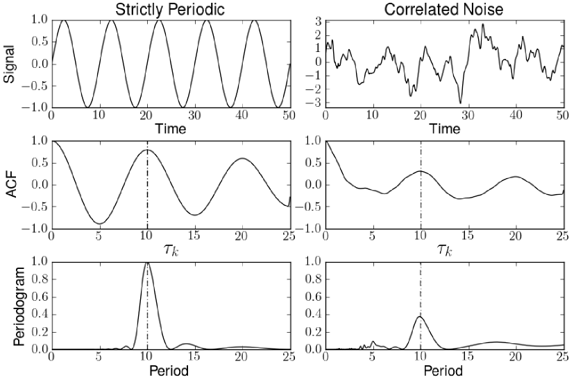
Figure 1: Simple synthetic signal of amplitude 1 (top row), and corresponding ACF (centre row) and periodogram (bottom row). The right hand column shows the effect of introducing noise of amplitude 0.9, correlated on a 2 time unit timescale. On the ACF and the periodogram panels, the input period used to generate the signal is shown as a vertical dotted line, detected period from each corresponding method is marked as the over-plotted dashed line.

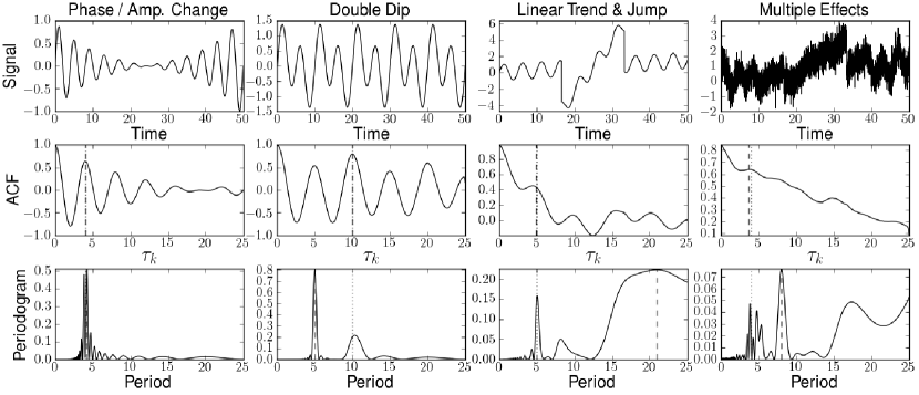
Figure 2: Synthetic examples showing the effects of varying signal phase and amplitude and injecting noise and systematics into the sine curves (top row), on the ACFs (middle row) and periodograms (bottom row). The ‘Multiple Effects’ signal comprises of the ‘Phase/Amp. Change’ signal from the first column, with injected white noise, correlated noise, a linear trend and a jump. On the ACF and the periodogram panels, the input period used to generate the signal is shown as a vertical dotted line, detected period from each corresponding method is marked as the dashed line, overlaying the dotted line in most cases.

In Fig. 2 we demonstrate how the ACF and the periodogram are affected by varying signal phase and amplitude, systematics effects and noise.

In cases where the phase and amplitude of the signal vary with time, the correct period is detected but the ACF peak amplitude varies within an envelope, corresponding to the amplitude variation of the signal. The peak width and level of symmetry can also vary. In this case, the periodogram produces two peaks on both sides of the correct period.

If the signal contains multiple minima and maxima per period, as can occur for spotted stars with more than one dominant active region, the ACF often shows alternating low and high ACF peaks, due to a partial correlation between the sets of maxima or minima. Our algorithm is built to identify these cases (see Section 2.1), and in this case selected the right period. On the other hand, the periodogram picked half the right period.

A jump or long term trend in the signal introduces a long term trend in the ACF, and since this can take many shapes, it is important to look at the local variations in peak height when performing diagnostics on the ACF. These long term trends introduce a long-period peak in the periodogram, which can lead to a wrong identification of long periodicity. We therefore expect the ACF method to be more reliable in these cases.

Noise and systematics are present in many stellar light curves displaying rotational modulation, and must be accounted for when attempting to determine rotation periods using the ACF. The effect of combining these factors is shown in the right column of Fig. 2, which has phase and amplitude modulation, white and correlated noise, a linear trend and a jump.

In summary, because the ACF measures only the degree of self-similarity of the light curve at a given time lag, the period remains detectable even when the amplitude and phase of the photometric modulation evolve significantly during the time-span of the observations. The ACF method is also capable of producing robust results in cases with residual instrumental systematics, because correlated noise, long-term trends and discontinuities give rise to monotonic trends in the ACF, on top of which we are able to identify the local maxima. Therefore, the ACF method is expected to be more robust to active region evolution than the periodogram, which implicitly assumes a stable, sinusoidal signal. The analysis of the real Kepler data supports this conclusion, as detailed in Section 3.6.

2.1 Measuring periods from the ACF

The period measurement involves three steps: identifying peaks in the ACF, selecting the peak associated with the mean rotation period, if any, and evaluating the uncertainty on the period.

The presence of high-frequency noise in the light curves leads to numerous local extrema in the ACF. Therefore, we first smoothed the ACF by convolving it with a Gaussian kernel, of window size of 56 lags and a full width at half-maximum (FWHM) of 18 lags. These values were tuned to provide the best compromise between reducing noise and maintaining ACF signal, without prior knowledge of the period. See Fig. 3 for an example of the effects of the smoothing treatment. We then identify local extrema in the smoothed ACF, defined as locations where the gradient changes sign.

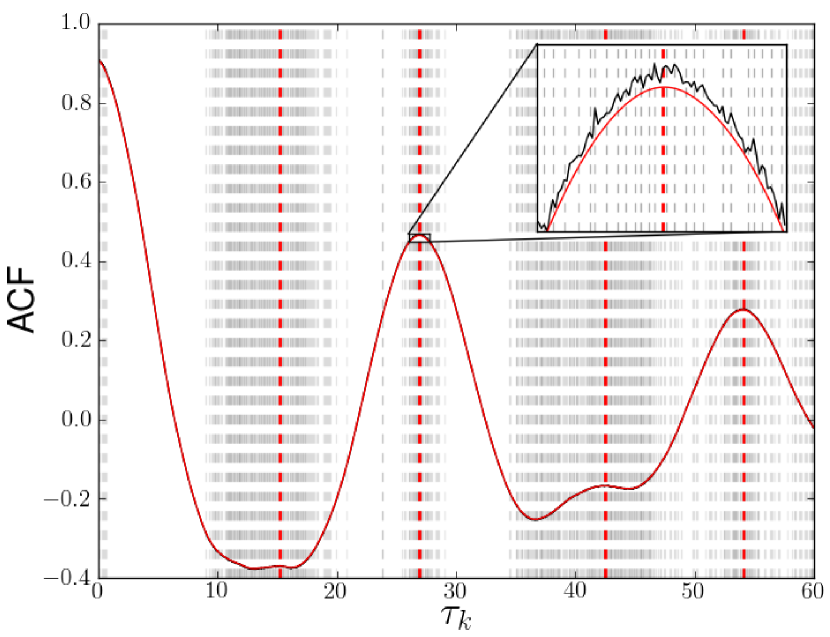
Figure 3: Example of an unsmoothed ACF (black curve) and corresponding smoothed curve (red). The many small peaks detected in the unsmoothed curve are shown as grey vertical dashed lines and the peaks detected from the smoothed version are shown as red vertical dashed lines. The inset plot shows a section of the ACF in detail.

If the light curve contains a clear rotational modulation signal, this process yields a series of clear, regularly spaced peaks of gradually decreasing height, as seen in Fig. 1. The first peak corresponds to the interval between patterns in the light curve, which evolve gradually, but are clearly repeated, and is thus identified as the rotation period. Some of the light curves contain long term trends and discontinuities, as a result of imperfections in the systematics correction. These introduce power at low frequencies, and thus affect the behaviour of the ACF for large lags, but the first ACF peak still corresponds to the correct period (as identified by visual examination of the light curve).

In the remaining steps, we make use of the height of the ACF peaks. However, correlated noise and residual systematics can introduce underlying long term trends, which mean the absolute peak height is no longer a good diagnostic. To mitigate this effect, we measure the height of each peak relative to the two adjacent minima, and adopt the mean of the two measurements as the ‘local height’ of the peak, denoted by $h_{\rm P}$. Since the ACF values range from -1 to 1, $h_{\rm P}$ has a positive value, of maximum 2.

If a star has two dominant active regions located on opposite hemispheres, each causes a series of dips in the light curve, approximately in anti-phase with each other. This gives rise to a partial correlation at half the mean rotation period, leading to a peak in the ACF at $\tau_{k}=P/2$. However, the peak at $P/2$ is typically smaller than that at $P$, because the two active regions do not generally give rise to identical dips. We therefore adopt the following condition: if $h_{\rm P}$ of the second peak is greater than that of the first, the second peak is selected instead. The right panel of Fig. 4 and the top left panel of Fig. 5 show a synthetic and real example of this effect, where this method has detected the correct peak.

In some cases, correlated noise and residual systematics produce an underlying slope at small $\tau_{k}$, causing a shift the position of the first peak associated with the rotation period. This occurs because a peak on a slope will have its maxima shifted in the direction of increasing gradient, as seen in the left panel of Fig. 4. To avoid this bias, a more robust period measurement is obtained using the median of the intervals $\Delta\tau_{k}$ between consecutive ACF peaks associated with the rotation period. To avoid selection of erroneous peaks, only those located at or close to (within 20%) of integer multiples of $\tau_{k}$ of the selected peak are used. If there are several locations selected around each peak (i.e. the smoothing has failed to remove all erroneous peaks), the peak selection only occurs after a gap of $\Delta\tau_{k}>0.3\ \tau_{k}$. This ensures only 1 data point per peak is used in the period measurement. Since the accuracy of the peak positions can decrease for very large $\tau_{k}$, a maximum of 10 peaks was selected for measurement of the median period and uncertainty.

We define the period uncertainty as the scatter of the $\Delta\tau_{k}$. Specifically, we used

$$\sigma_{P}=\frac{1.483\times\rm{MAD}}{\sqrt{N-1}}$$ (3)

where $N$ is the number of peaks, and MAD is the median of the absolute deviations from the median $\Delta\tau_{k}$. This ‘MAD-estimated scatter’ is equivalent to the standard deviation for a Gaussian distribution, but is more robust to outliers. In cases where we identified only one peak matching the selection criteria, we adopt the peak position as the period and the half width at half local peak height as the period uncertainty.

2.2 Tests with Realistic Light Curves with Injected Simulated Stellar Modulation

To demonstrate the robust nature of the ACF, we present a selection of synthetic examples with known input parameters. A more detailed evaluation of the method over the full range of parameter space will be described in future work.

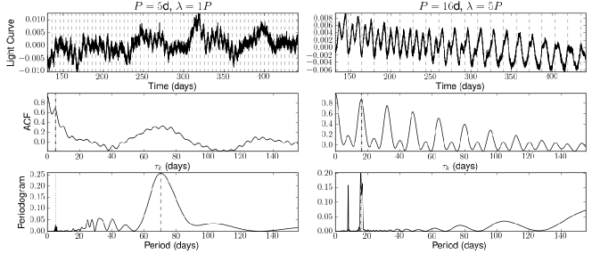
Figure 4: Examples of synthetic light curves and corresponding ACFs and periodograms for different input parameters, indicated in the plot titles. In the left panel the spot distribution was selected to give a double-dip light curve. The dashed lines on the light curve plots indicate intervals at the period detected by the ACF. On the ACF and periodogram plots, the input period is marked by a dotted line and the detected period is marked by a dashed line.

To generate synthetic light curves we used a simple spot model code, described in Aigrain et al. (2012), which takes the following input parameters: number of spots, light curve amplitude, characteristic spot half-life ($\lambda$), light curve duration, fractional differential rotation, inclination and time sampling.

The observations of Jackson & Jeffries (2012) show that activity is better explained by a large number of small spots, than a small number of large spots. They suggest a spot number of 2500-5000, however, since they observe younger stars we opt for a smaller spot number of 200. This also increases the speed of synthetic light curve generation. We selected an amplitude of 1% and an inclination angle of $75^{\circ}$. The time sampling and duration match that of the Kepler Q1-4 data.

Since the effects of the noise and residual systematics of the Kepler data are an important factor when analysing the ACF, we introduce these into the synthetic light curves. A random selection of the Kepler M-dwarf light curves were visually examined and 10 were selected which appeared to contain only noise and systematic effects, with negligible intrinsic stellar signal. For each synthetic output, we created 10 light curves with realistic noise and systematics by adding each of the selected quiet Kepler light curves.

The two synthetic examples in Fig. 4 demonstrate the ability of the ACF to recover the input period from quite difficult cases, where the periodogram failed to identify the right period.

The many synthetic cases we tried led us to believe that the ACF method and the periodogram are less reliable for light curves with very fast spot evolution ($\lambda\,\textless\,1$ period), short periods ($\textless\,7$ days) and strong systematics. This is caused by the steep initial slope in the ACF, combined with the smoothing algorithm, which masks the peaks. Similarly for fast evolution, strong systematics and long periods ($\textgreater\,35$ days), the ACF peaks are too strongly affected by underlying trends. The periodogram suffers mainly from spurious peaks at long periods.

As the spot half-life is increased to 1 period, the periodic signal strength increases, and by $\lambda$ = 5 periods, the majority of periods are correctly detected, across the range of input values. It should be noted that these synthetic examples were designed to test the limits of the ACF and therefore all have a low signal to noise. A recent study of a sample of Sun-like stars observed by CoRoT (Mosser et al., 2009) found that spot lifetime of the order of the rotation period are not atypical for Sun-like stars. On the other hand, the spot lifetime is also known to increase with increased activity level (Hall & Henry, 1994).

2.3 Amplitude of variability

To estimate the average amplitude of the periodic signal, we use a modified version of the range statistic $R_{\rm var}$ defined by Basri et al. (2010, 2011) and McQuillan et al. (2012), which is the interval between the $5^{\rm{th}}$ and $95^{\rm{th}}$ percentiles of the light curve. This rank-order approach enables us to quantify the amplitude of the variability without specifying a particular model for it, and excluding the extreme values minimises the sensitivity to outliers and high-frequency noise. We divide the light curve into segments, whose duration is equal to the detected period, measure $R_{\rm var}$ separately in each of them, and define $R_{\rm per}$ as the average of the $R_{\rm var}$ measurements obtained in this way. In most cases, $R_{\rm per}$  is very similar to the $R_{\rm{var}}$ value for the whole light curve.

3 Application to Kepler Data M-Dwarfs

3.1 Target Selection

Following Ciardi et al. (2011), we selected M-dwarfs among the Kepler targets based on the effective temperature $T_{\rm eff}$ and surface gravity $\log g$ reported in the Kepler Input Catalog, or KIC (Brown et al., 2011). These parameters were estimated using Bayesian posterior probability maximisation (Brown et al., 2011), matching observed colours, estimated from Sloan $g$, $r$, $i$, $z$ filters, 2MASS $JHK$, and D51 (510 nm), to the stellar atmosphere models of Castelli & Kurucz (2004), resulting in typical uncertainties of $200\,$K for $T_{\rm eff}$ and $0.5$ dex for $\log g$, respectively. These are the typical errors for each parameter, but the actual errors may vary by a small amount between stars of different magnitude and spectral type. For a more detailed discussion of the KIC parameters, see Brown et al. (2011), Batalha et al. (2010) and Verner et al. (2011). There is increasing evidence that the KIC values for the radii and $T_{\rm eff}$ are overestimated (e.g. Mann et al., 2012; Verner et al., 2011; Muirhead et al., 2012), which means the values of $T_{\rm eff}$ should be interpreted with care.

This study focusses on M-dwarfs stars, which were selected following Ciardi et al. (2011) as having $T_{\rm eff}\leq 4000$ K and $\log g\geq 4.0$ dex, manually adding 25 known M-dwarfs (Ciardi et al., 2011) with missing KIC parameters. Table 1 summarises the number of stars considered at each stage of the study.

Table 1: Number of objects included at each stage of the study. The column labelled ‘All dM’ includes both M-dwarfs selected from the KIC parameters and the previously known M-dwarfs without KIC parameters. The totals in the second column include the known EBs and planet candidate host stars, which are also listed separately in the last two columns. The possible giants and double-period stars were removed from the final results reported in Tables 2 & 5. Note: removed 4 contact EBs from Q1-4 EB selection.

Stage	All dM	EBs	Pl. host
KIC selection	2937	15	57
Q1-4 light curves	2483	9	51
Period detected	1730	7	42
Possible giants	121	0	0
Double-period	39	0	0
Binaries or pulsators	112	-	0
Final periodic total	1570	7	42

3.2 Obtaining and pre-processing the light curves

This study is based on public release 14, which was available when the present analysis was performed. The release included data from Quarter 1 (Q1) to Quarter 4 (Q4) of Kepler observations, which took place over $\sim 310$ days between May $13^{\rm th}$ 2009 and March $19^{\rm th}$ 2010. Approximately $156\,000$ targets were observed during this time, most with a cadence of $29.42$ minutes. These data are publicly available and were downloaded from the Kepler mission archive (http://archive.stsci.edu/kepler) at the Space Telescope Science Institute (STScI).

Public release 14 included a re-processing of Q1– Q4 with a new version of the presearch data conditioning (PDC) pipeline known as PDCMAP. The purpose of the PDC is to remove the majority of instrumental glitches and systematic trends. In contrast with earlier versions, the new PDC-MAP uses a Bayesian approach to do so while retaining most real (astrophysical) variability (Smith et al., 2012; Stumpe et al., 2012). It works very well for Q3 and Q4, but some artefacts remain in some light curves in Q1 and Q2. Improving the correction of instrumental effects further remains an important goal to enable the full exploitation of Kepler’s potential in terms of stellar astrophysics. However, in the vast majority of the cases we have examined, the residual artefacts in the PDC-MAP data do not prevent the detection of rotational modulation, so we consider it suitable for the present work.

An additional 5 quarters of PDC-MAP data were made publicly available a few weeks before the submission of this manuscript. We are planning to analyse these in the near future, in the hope that it will improve our sensitivity to long periods, but we do not expect it to affect the main conclusions of this paper.

The ACF calculation requires the light curves to be regularly sampled and normalised to zero. We divided the flux in each quarter by its median and subtracted unity. Gaps in the light curve longer than the Kepler long cadence were filled using linear interpolation with added white Gaussian noise. This noise level was estimated using the variance of the residuals following subtraction of a smoothed version of the flux. To smooth the flux we applied an iterative nonlinear filter which consists of a median filter followed by a boxcar filter, both with 11-point windows, with iterative 3-sigma clipping of outliers.

This method of gap filling and quarter stitching was only found to introduce spurious jumps in light curves for which the systematics correction had failed, and were therefore already problematic. In the vast majority of cases, the amplitude of M-dwarf activity mean that any quarter stitching effects have a negligible impact on the period detection.

Our sample also includes a number of previously identified eclipsing binaries and planetary transit candidates (Prša et al., 2011; Batalha et al., 2012). In those cases we cut out and interpolated over the eclipses/transits before performing the rotation period search.

3.3 Establishing confidence in the period detection

Given the scientific importance and manageable size of the sample under study here, we opted to perform a visual examination of all the light curves in order to verify the period detected by the ACF. The light curves were compared to dashed vertical lines at intervals of the detected period (see e.g. Fig. 5). In order to classify the detection as valid, features in the light curve must be present at intervals matching the dashed lines, across several periods, preferably in more than 1 quarter.

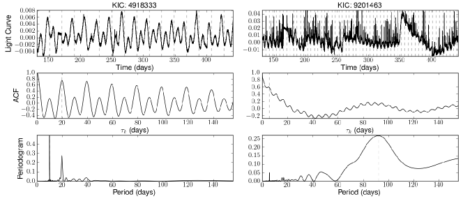
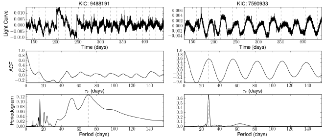
Figure 5: Examples of Kepler light curves and corresponding ACFs. The dashed lines on the light curve plots indicate intervals at the period detected by the ACF (dashed line on ACF plot). KIC 4918333 shows two active regions, creating a double dip effect. The correct period was automatically detected by selecting the second (higher) ACF peak. KIC 9201463 shows that the ACF is robust against flares and significant systematics. KIC 9488191 contains significant residual systematics and the effect on the ACF is apparent, however, the correct period is still detected. KIC 7590933 shows an example which has been marked as ’possible harmonic’ or ‘HM’ in Table 2, since it is not clear whether the rotation period corresponds to the first or second ACF peak, even though the ACF peak height indicates it should be the first (see text for further discussion).

We paid particular attention to the question of whether the detected period was clearly the rotation period, or could be $P/2$, as described in Section 2.1. In 73% of light curves we identified features which could be ‘tracked’ visually, i.e. a particular shape of spot crossing that repeats throughout the light curve. When there are more than one such sets of features, and they evolve gradually relative to each other, as shown for example in the top left panel of Fig. 5, the rotation period is very clear. When only one such set is visible and the first ACF peak is not higher than the second (e.g. the bottom right panel of Fig. 5), we cannot be so certain, but the simplest explanation is nonetheless that the detected period is correct. In around 1% of the cases where we report a period, there is very tentative evidence in the light curve that the detected period is a harmonic (i.e. $P/2$), but we could not be certain, so we simply flagged the corresponding objects as ‘possible harmonics’. Such cases may be resolved once additional quarters of Kepler data are incorporated into the analysis. We note that these cases are not numerous enough to explain the two sequences seen in the period-temperature diagram (Fig. 10), and are spread across the entire period range.

In 3.6% (57) of the periodic cases an incorrect peak was identified. This was most frequently a result of noise introducing extra peaks, or very large residual systematics changing the relative peak heights. These cases were manually corrected to select peaks corresponding to the period identified by eye.

In the future, we plan to apply the same analysis to a much larger sample of Kepler targets (including F, G and K dwarfs), for which an automated detection method must be developed. The present, visually inspected subset will then prove valuable, to validate any threshold to be applied automatically to a larger sample. Here we merely note that, in the present study using 10 months of data, it is possible to recover 91% of our detections, at the cost of a false alarm rate of 10%, by selecting objects with

$$h_{\rm P}>{\rm MAX}\left(0.15,\frac{\sigma_{\rm P}}{51\,{\rm days}}\right).$$ (4)

3.4 Results

Table 2: M-dwarfs with detected rotation periods. This table is available in its entirety, in a machine-readable form in the online supplementary material, or at http://www.physics.ox.ac.uk/StellarRotation. A portion is shown here for guidance regarding its form and content. $T_{\rm eff}$ and $\log g$ are from the KIC and $M$ was derived from $T_{\rm eff}$ using the 600 Myr isochrone of Baraffe et al. (1998). The average amplitude of variability per period bin of the light curve, $R_{\rm per}$, is included. The meaning of the flags are: ‘EB’: known eclipsing binary (Prša et al., 2011); ‘PL’: planet host candidate (Batalha et al., 2012); ‘PB’: ultra-stable periodic behaviour, indicating possible binary, pulsator or young object; ‘HM’: the reported period may be a harmonic of the true period; ‘NF’: no flag.

KIC	$T_{\rm eff}$	$\log g$	$M$	$P_{\rm rot}$	$\sigma_{\rm P}$	$R_{\rm per}$	Flag
	(K)	(g/cm3)	($M_{\odot}$)	(days)	(days)	(mmag)
1162635	3899	4.62	0.5037	15.509	0.064	10.7	NF
1430893	3956	4.41	0.5260	17.144	0.046	10.4	NF
1572802	3990	4.48	0.5394	0.368	0.000	74.8	PB
1721911	3833	4.58	0.4781	28.403	0.394	3.9	NF
1866535	3878	4.50	0.4955	25.052	0.136	4.0	NF

We applied the ACF method and visual inspection steps described in the previous section to the Kepler light curves of the objects selected as likely M-dwarfs. The results are reported in Tables 2 to 5. The full machine-readable tables are available in the online supplementary material, or with plots of every light curve, its ACF, and sine-fitting periodogram at the URL http://www.physics.ox.ac.uk/StellarRotation. Table 2 reports all our period measurements, except for two groups of objects, listed separately in Tables 3 and 4, which were excluded from the sample for reasons detailed below. Table 5 lists all the objects which passed our target selection criteria, but for which no period was detected. The final number of likely M-dwarfs with detected rotation periods is 1570 (out of the 2483 light curves we analysed, or 2362 if we discount objects later found to be giants).

3.5 Excluding non-rotators

Rotational modulation of star spots is not the only cause of periodic, or quasi-periodic, variability in stellar light curves. The visual examination stage was therefore important in identifying groups of stars whose variability did not appear to be caused by rotation, or by rotation alone.

The Kepler light curves have already been searched extensively for planetary transits (Borucki et al., 2011; Batalha et al., 2012) and stellar eclipses (Prša et al., 2011). We included these objects in our sample, after removing the transits and eclipses, as described earlier. Measuring the photometric rotation periods of known binaries is useful to check for differences between the rotational properties of close binaries and of apparently single stars. The rotation of planet-host stars is an important topic in itself, which is beyond the scope of the present paper and will be investigated in detail in a forthcoming publication.

Table 3: Objects identified as likely giants from their light curves. This table is available in its entirety, in a machine-readable form in the online supplementary material, or at http://www.physics.ox.ac.uk/StellarRotation. A portion is shown here for guidance regarding its form and content.

KIC	$M$	$\log g$	$T_{\rm eff}$	$R_{\rm var}$
	($M_{\odot}$)	(g/cm3)	(K)	(mmag)
1026895	0.5343	4.53	3977	8.99
1160867	0.4474	4.57	3753	8.29
1431599	0.5068	4.5	3907	12.68
1576043	0.4889	4.52	3861	7.76
2010137	0.4881	4.48	3859	7.01

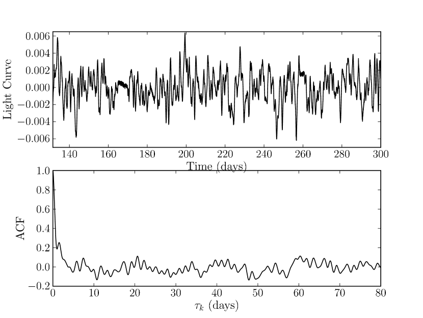
Figure 6: KIC 2010137 is an example of a star which we identified as a likely giant based on its light curve, which shows stochastic variability with a clear, dominant time-scale, but no repeatability, and does not resemble the signal expected from rotation.

One distinct group of 121 stars show a clear ACF peak at relatively short $\tau_{k}$ ($\sim 1$–$12$ days), but there are few additional peaks at integer multiples of the first, and the light curve appears stochastic rather than truly periodic. Such an example is shown in Fig. 6. We initially thought that these objects may be rapid rotators with very rapidly evolving active regions, or a hitherto unidentified type of pulsating star. We examined their KIC parameters, and noted that they appear redder, and have lower proper motions, than the rest of the sample. We therefore concluded that they are likely to be giants contaminating our sample. Indeed, if we apply the $J-H<0.75$ cut advocated by Ciardi et al. (2011), it removes 117 stars from the M-dwarf sample, of which 103 belong to this group of objects displaying stochastic behaviour. We therefore concluded that these objects are likely giants, removed them from the M-dwarf sample and list them separately in Table 3.

A further 39 objects display evidence for two, very distinct periods in their light curves, with one period several times longer than the other. This could potentially result from the light of two different variable stars being included in a single photometric aperture, which may be revealed by examination of the pixel level data. Since the nature of the periodicity is unknown, and the determination of the KIC parameters used to select these objects as M-dwarfs could be affected by the presence of a close companion, we exclude these objects from our sample, and list them separately in Table 4. Note we do not report periods for them, because the presence of two distinct signals in their light curves makes the identification of either period more challenging.

Figure 7: Examples of the objects classified as ‘PB’. KIC 5516671 (top) shows a very stable light curve and KIC 3103752 (bottom) shows the ‘beat pattern’ discussed in the text.

Table 4: Objects with two distinct periods in their light curves. This table is available in its entirety, in a machine-readable form in the online supplementary material, or at http://www.physics.ox.ac.uk/StellarRotation. A portion is shown here for guidance regarding its form and content.

KIC	$M$	$\log g$	$T_{\rm eff}$	$R_{\rm var}$
	($M_{\odot}$)	(g/cm3)	(K)	(mmag)
892376	0.4704	4.47	3813	13.84
1569863	0.4688	4.45	3809	33.94
2557669	0.4585	4.36	3782	37.7
3646734	0.4372	4.47	3726	25.89
3735772	0.4414	4.48	3737	85.71

Finally, 109 stars show unusually stable periodic behaviour, with periods typically $<7$ days, and very little or no evidence of any evolution over the full Q1–Q4 duration. Some of these also show a beat pattern characteristic of the light curves containing two, mutually similar periodicities. See Fig. 7 for examples. These objects could be members of close binary systems, where the active region pattern is stabilised over long timescales because of the presence of a companion. Their rotation periods and amplitudes are certainly similar to those of the known eclipsing binaries in the sample. If they are binaries, the beat patterns may indicate differential rotation on one of the stars, or two slightly different rotation periods for the two components of the binary. We are not aware of any type of main-sequence M-dwarf that would be expected to pulsate in this period range, but we cannot rule out binarity or pulsation without spectroscopy. We therefore kept these objects in Table 2, but flagged them as ‘binaries or pulsators’, indicating their period may result from a phenomenon other than rotation.

Table 5: Objects with no rotation period detection. This table is available in its entirety, in a machine-readable form in the online supplementary material, or at http://www.physics.ox.ac.uk/StellarRotation. A portion is shown here for guidance regarding its form and content.

KIC	$M$	$\log g$	$T_{\rm eff}$	$R_{\rm var}$
	($M_{\odot}$)	(g/cm3)	(K)	(mmag)
1160684	0.5244	4.48	3952	3.35
1292688	0.5146	4.86	3927	7.48
1569682	0.5154	4.69	3929	4.99
1718059	0.526	4.49	3956	3.13
1718071	0.5225	4.54	3947	5.77

3.6 Comparison of the AFC and sine-fitting periodogram

We computed sine-fitting periodograms for the sample of Kepler M-dwarfs using 1000 logarithmically-spaced periods between 0.1 and 155 days.

In general, similar results are obtained from the ACF or periodogram methods, however, we consider the ACF clearer and more reliable. A useful feature of the ACF method is that it enables automatic identification of cases where the detected period is a half the mean rotation period. An example of this is shown for KIC 4918333 in Fig. 5, which clearly shows that the mean rotation period corresponds to the second ACF peak, whereas the first periodogram peak is the highest.

Similarly, for KIC 9488191 in Fig. 5, one can determine easily from the ACF that the rotation period corresponds to the first peak at $\sim 15$ days and not the highest peak in the periodogram at $\sim 70$ days. Although long period peaks could be excluded from the periodogram to allow the correct peak to be selected, this would require prior knowledge of the possible range of rotation periods to avoid removal of genuine long period signatures.

A more systematic comparison between the ACF and periodogram results is shown in Fig. 8. Here we make a one-to-one comparison of the periods detected using the ACF and the sine-fitting periodogram, for all the cases where the light curves were determined to show periodic variations from visual examination.

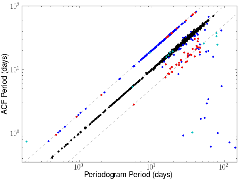
Figure 8: Comparison of the periods detected using the ACF and the periodogram, for all stars with a visually confirmed periodicity and ACF detection. The correct ACF detections where the periodogram detections are within 10% of the ACF period are shown in black (1298), the cases where the periodogram period is not within 10% of the ACF period are shown in dark blue (215). Cases where the ACF initially selected the wrong period but the periodogram selected the correct one are marked by red points (45). Cases where both the ACF and periodogram detected the wrong period are marked as cyan points (12). The grey dashed lines show where $P_{\rm ACF}=P_{\rm LS}$, $P_{\rm ACF}=2\times P_{\rm LS}$ and $P_{\rm ACF}=0.5\times P_{\rm LS}$.

In 222 (14%) of the periodic cases, the periodogram does not detect the correct period (to within 10%). The most common discrepancy arises from cases where the periodogram has detected half the period of the ACF (170 cases). We stress that there is no obvious way of identifying these cases automatically using the periodogram alone (for example, we tried to use the relative heights of the periodogram peaks, without success). In 11 cases the periodogram selects erroneous long period peaks and the ACF selects the correct shorter period peak.

On the other hand, the ACF yielded 57 incorrect ACF period detections (3.6%), 45 cases occur where the ACF method selects the wrong period, and the periodogram selects the correct period. These cases are marked as red points in the Figure 8. For the remaining 12, both the ACF and periodogram detect the wrong period (cyan points).

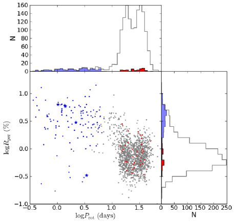
Figure 9: Period versus amplitude for the rotating Kepler field M-dwarfs. Blue dots represent objects with $P_{\rm rot}<10$ days, which also display unusually stable modulation patterns in their light curves, and blue stars known, short-period eclipsing binaries (Prša et al., 2011). Red dots represent the host stars of candidate transiting planets (Batalha et al., 2012). All the other M-dwarfs with detected rotation periods are shown as grey dots. The histograms of each parameter are shown along the corresponding axis, with matching colours. Two long-period binaries are not shown as blue stars in the plot.

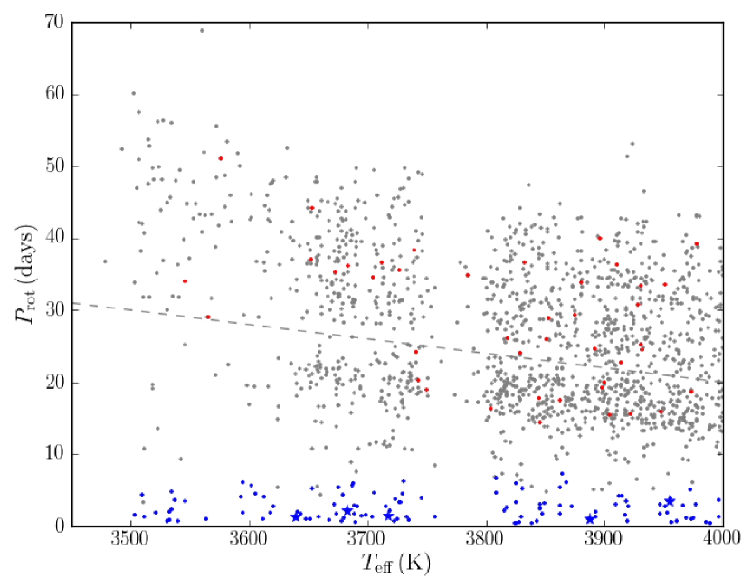
Figure 10: Period versus effective temperature for the rotating Kepler field M-dwarfs. The symbols and colours as the same as in Fig. 9.  The apparent dearth of objects around $T_{\rm eff}=3775$ K is not apparent in any of the KIC colours, and is therefore thought to be a result of the KIC stellar parameter estimation procedure, rather than a real effect. The dashed line marks the location of the cut made by eye between the fast and slow rotators.

In one case (KIC 10553513, not included in the periodic sample), the large residual systematics prevent either the ACF or the periodogram from detecting the rotation period which is visible in the light curve. The only case for which the periodogram is able to detect the period and the ACF is not (even with manual correction) is KIC 5480340 (not included in the periodic sample). This is due to the extremely short period (0.25 days). The steep gradient in this region of the ACF prevents peak detection, which we plan to resolve in a future version of the algorithm.

We conclude that the periodogram remains a valuable technique for period detection, however the clarity and robustness of the ACF method makes it our tool of choice for the measurement of stellar rotation in light curves. The ACF method works independently of periodogram based methods and is ideal for determining rotation period statistics for large datasets.

4 Discussion

4.1 Period, amplitude and temperature

We now examine the period distribution of our sample as a function of amplitude (Fig. 9) and effective temperature (Fig. 10). A number of interesting features are immediately apparent.

First, the period distribution is clearly bimodal for $P_{\rm rot}>10$ days, with peaks of approximately equal height at $\sim 19$ and $\sim 33$ days. This bimodality appears statistically significant in log period space, with a Hartigan’s dip test $p$-value of 0.0003 (Hartigan & Hartigan, 1985). The two peaks of the rotation period distribution form two distinct sequences in period-temperature space (Fig. 10). The period decreases with increasing temperature, in much the same way, for both sequences. This variation as a function of temperature implies the gap between the sequences is not a result of systematics in the Kepler light curves leading to missed detections in a particular period range. We define the short and long period samples based on the line, plotted somewhat arbitrarily, shown in Fig. 10.

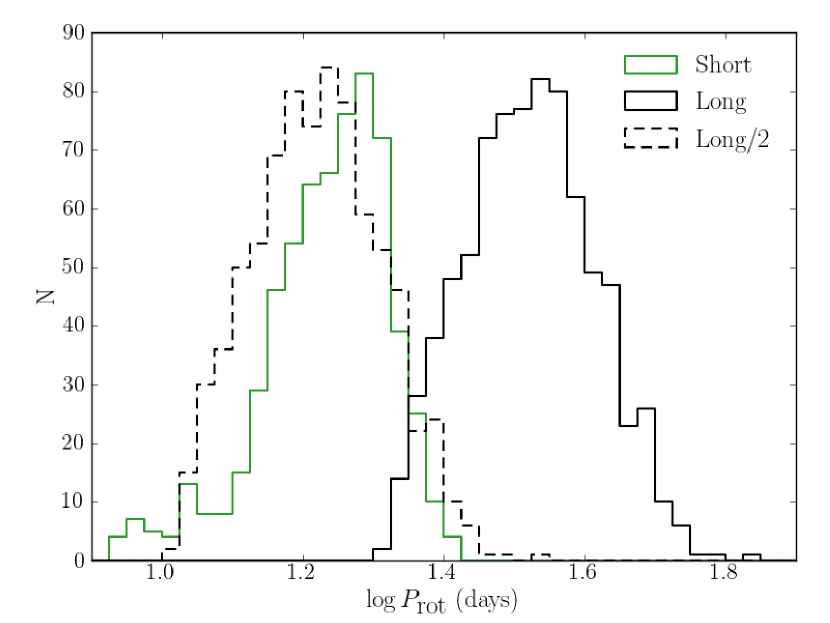
Figure 11: Histogram of the short and long period M-dwarfs, as defined by the cut marked with the dashed line in Fig. 10. The dashed histogram marks the long periods divided by 2, and provides further evidence that the short period set are unlikely to be erroneous half-period measurements of the long period population.

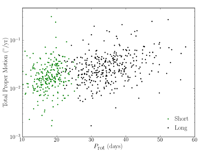
Figure 12: Total proper motion against Period for the short period (green) and long period (black) M-dwarfs, as defined by the cut marked with the dashed line in Fig. 10.

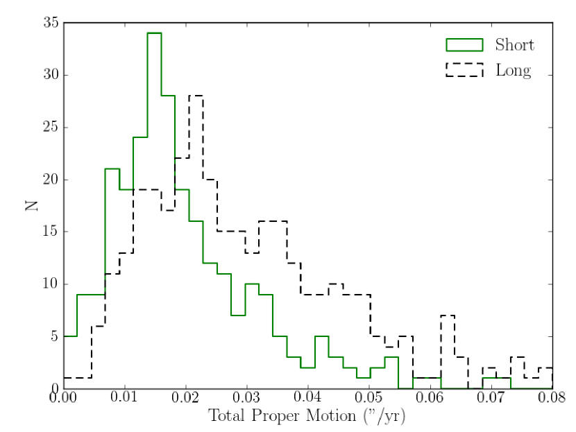
Figure 13: Histogram of the total proper motion for the short period and long period M-dwarfs, as defined by the cut marked with the dashed line in Fig. 10. The uncertainty on the proper motion values is 0.02”/year but given the high numbers in each sample these results are still significant. The known and ‘possible’ binaries have been removed from this sample (blue points and stars in Fig. 10).

Before interpreting this result, we must address the possibility that the bimodal distribution is spurious: an error of a factor of two in the periods of about half the objects could give rise to the observed distribution. Such errors are not uncommon in rotational studies based on ground-based data (see e.g. Collier Cameron et al., 2009). However, they are less likely to be prevalent in the present study, for the following reasons. We can exclude a scenario where we measured twice the true period for the objects belonging to the longer period peak, because of the continuous sampling of our data. The alternative scenario is that we measured half the true period for the objects belonging to the shorter period peak. This kind of problem arises when the brightness distribution of the stellar surface is bimodal, due to concentrations of active regions on opposite hemispheres, resulting in ‘double-dip’ light curves. However, our ACF peak selection routine was specifically designed to address this problem – this is one of the strengths of the method. In fact, for 210 of the objects belonging to the shorter period peak, a ‘double-dip’ light curve lead to the second ACF peak being automatically selected as the rotation period. Unless these stars have quadrupolar surface brightnesses, it is very unlikely that we underestimated their periods by a factor of two.

The case for genuine bimodality is further strengthened by comparing the detected distribution to that which would arise if either set were wrong by a factor of 2. Fig. 11 shows that division of the long period set by 2 does not reproduce the short period set (and equivalently neither does multiplication of the short period group). A quantitative two-sample Kolmogorov-Smirnov (KS) test of the short period sample and the long period sample divided by 2 gives a p-value $9\times 10^{-14}$, confirming they are very unlikely to be drawn from the same distribution.

Fig. 12 shows a weak correlation between period and total proper motion for the two samples. We also see tentative evidence of a difference in the proper motion distributions of the short and long period samples. Fig. 13 shows the histograms for stars in the short and long period samples with non-zero proper motion KIC measurements (266 short, 345 long). The proper motion values from the KIC are taken from a selection of catalogs where available. Total proper motion is listed on NStED as having accuracy of 20 milliarcseconds per year, but the large number of objects in each sample support the difference between them.

We also checked for differences in the galactic latitude and Kepler magnitude distributions of the two samples but did not see any clear differences. By using the galactic latitude measurements and an approximate distance estimate from average apparent and observed M-dwarf magnitudes, we conclude that the observed population lies within a small fraction of the scale height of the thin disk, and therefore a variation of properties with Galactic latitude is not expected.

For the remainder of this study, we therefore assume our sample contains two distinct stellar populations. The gap between the two sequences in Fig. 10 is reminiscent of the Vaughan-Preston gap (hereafter, V-P gap) found by (Vaughan & Preston, 1980, hereafter, VP80) when studying the chromospheric activity levels of a relatively small sample of F and G stars as a function of $B-V$ colour. As chromospheric activity, like stellar rotation, declines with age, both observed gaps suggest two waves of star formation in the Solar neighbourhood, as discussed by VP80 themselves and by numerous authors subsequently (see, for example, Barry 1988, Pace & Pasquini 2004 and references therein). Alternative explanations for the V-P gap include a discontinuity in the chromospheric activity level or of the rotation period at a particular point in the star’s evolution. Noyes et al. (1984) found no evidence for a difference in the relationship between chromospheric activity, rotation period and colour for stars on either side of the V-P gap, which led them to dismiss the first of these alternatives. Our results also suggest the gap does not result from a discontinuity in the chromospheric activity level, as we see no obvious difference in the amplitude of photometric variability of the slow and fast rotators. Of the two remaining hypotheses, that of two waves of star formation seems more plausible, and is supported by the tentative differences we observe between the proper motion distributions of the two groups, but more kinematic data would be needed to confirm different epochs of star formation.

The fact that these have different median periods and different proper motion characteristics suggests that they may result from two distinct waves of star formation: as already discussed, low-mass main-sequence stars spin down as they age, and older populations tend to have larger velocity dispersions than younger populations, due to dynamical heating of the Galactic disk over long timescales (see Freeman & Bland-Hawthorn, 2002, and references therein). The ratio of the two peaks in the period distribution corresponds to an age ratio of $\sim 3$, if one assumes that M-dwarfs spin down as $t^{0.5}$, as observed for Sun-like stars (Skumanich, 1972). Recent rotational studies of low-mass stars in open-clusters suggest that the index of the spin-down low might be closer to $0.6$ (see e.g. Meibom et al., 2009), which would imply an age ratio of $\sim 2.5$. We note that an interpretation in terms of thin and thick disk populations is unlikely because there should be many fewer thick disk than thick objects in the Kepler sample, which is essentially magnitude-limited.

Further kinematic and distance information is required to draw stronger conclusions about the nature of the two populations. The Kepler mission itself may, in the medium term, provide this information: the pixel-level data can be used to monitor the centroid of each star over the full lifetime of the mission, which should enable the measurement of proper motions and parallaxes for some targets. Monet et al. (2010) shows that astrometric precision for a single 30 minute measure is $\textless\ 4$ milliarcseconds. In the longer term, the GAIA mission (de Bruijne, 2012) will provide this information with greater precision and for more objects.

While the bulk of the objects (89%) have periods in the range 10–50 days, a small fraction ($8\%$) of the periods are $<7$ days. Almost all these rapid rotators display unusually stable light curves over the full 10 month dataset (blue points in Figs. 9 and 10, label ‘PB’ in Table 2). Most of them also have relatively large amplitudes ($>2\%$, compared to 0.2–2% for the bulk of the sample). Two possible explanations spring to mind for these rapid rotators: they may be significantly younger than the rest of the sample (for example members of the young disk population, see Section 4.2), or they may be close binary systems, which have become rotators due to spin-orbit interactions. The 5 known short-period eclipsing binaries in our sample (shown as stars in Fig. 9) all display synchronised rotation signals, suggesting that at least some of the other However, we cannot conclusively distinguish between the two possibilities without spectroscopy.

Figure 14: Period versus mass for low-mass field stars. Based on data from Baliunas et al. (1996) and Kiraga & Stepien (2007) (circles) and MEarth data from Irwin et al. (2011) (stars), with grey and black symbols representing objects with young and old disk kinematics, respectively. Additional M-dwarf periods from the WFCAM Transit Survey (Goulding et al., 2012), for which no kinematic classification is available, are shown as white triangles. The new results from the present study are shown as blue points.

Finally, all the planet-host candidates (Batalha et al. 2012, red points in Figs. 9 and 10) have $P_{\rm rot}>10$ days and amplitude $<2\%$. If the period and amplitude distributions of the planet-host candidates were the same as those of the rest of the sample, we would have expected $\sim 3$ of them to have $P_{\rm rot}<10$ days and/or amplitude $>2\%$ (of all the M-dwarfs with rotation periods, $10\%$ fall outside these limits, and there are 42 candidate planet host stars in the sample). The number of objects concerned is too small to draw firm conclusions, but it does suggest that either the search for transits in Kepler light curves may be less complete around active, rapidly rotating stars, or that there are fewer transiting planets around these stars (which could be the case of the rapid rotators are close binaries). Either way, this should be taken into account when inferring the incidence of planets around different types of stars.

4.2 Period-mass relation

To compare our results with other rotational studies of low-mass stars, we estimated masses for the Kepler M-dwarfs from the KIC effective temperatures. Much of the previous work on rotational evolution (Kawaler, 1989; Barnes, 2003, 2007; Meibom et al., 2009; Collier Cameron et al., 2009) uses a directly observed colour index, such as $B-V$ or $J-K$, instead of model-dependent mass estimates, to confront models with observations. We opted for masses for three reasons. First, angular momentum evolution models generally depend on fundamental parameters rather than colours. Second, neither of the colour indices most frequently used, $B-V$ and $J-K$, is well matched to our targets, which are very faint in $B$, and have almost constant $J-K$ over the mass range of interest (in contrast to G and K-dwarfs, where $J-K$ is a steeper function of mass). Third, stellar parameters based on multi-colour photometry should be less sensitive to reddening than any single colour index.

The masses used in this study were obtained by interpolating the $630$ Myr isochrone of Baraffe et al. (1998). We checked that the results are essentially unchanged if the age is increased by a factor of up to 10. While useful for a general comparison, we stress that these masses are very uncertain and should not be used for individual objects. The $200\,K$ formal uncertainties on $T_{\rm eff}$ alone translate into mass uncertainties ranging from $0.15\,M_{\odot}$ (for $M\sim 0.3\,M_{\odot}$) to $0.1\,M_{\odot}$ (for $M\sim 0.6\,M_{\odot}$). Additionally, any systematic errors in $T_{\rm eff}$, discussed in Section 3.1 are automatically propagated through to the masses.

Fig. 14 shows the period-mass relation for field stars with masses below $1.3\,M_{\odot}$, based on a compilation of literature sources (Baliunas et al., 1996; Kiraga & Stepien, 2007; Irwin et al., 2011; Goulding et al., 2012). Our sample (small blue dots on Fig. 14) ties in smoothly with the existing data at both higher and lower masses (circles, stars and triangles). The tight sequence followed by old F, G and K stars is clearly seen on Fig. 14, as are the younger stars gradually evolving towards that sequence. This evolution is relatively well reproduced by simple models of angular momentum loss via a magnetised wind (Kawaler, 1988, 1989), and forms the basis for rotational age-dating, or gyrochronology (Barnes, 2003, 2007).

The picture is more complex for M-dwarfs, which evolve more slowly, and hence have not converged onto a common sequence, even after several Gyr. However, the new, much larger sample of early M-dwarfs strengthens two interesting features, which were only hinted at by previously published results.

First, we might have expected to see some kind of transition around $0.35\,M_{\odot}$ (Chabrier & Baraffe, 1997; Scholz et al., 2011), which corresponds to the transition between fully convective stars and stars with a radiative core, because the so-called interface dynamo, which powers the magnetic field of Sun-like stars, cannot operate in the absence of a radiative core. No such transition is seen among the slowly rotating stars, which define the upper envelope of the period-mass relation. There does seem to be a transition at $\sim 0.35\,M_{\odot}$ for rapid rotators: below this mass, rapid rotators persist even among kinematically old stars, as the MEarth sample of Irwin et al. (2011) illustrates, but above it, all the fast rotators are kinematically young, as Kiraga & Stepien (2007) pointed out. The Kepler sample as it stands cannot shed much additional light on this point because we currently lack kinematic and distance information.

Second, a transition that was not expected, but is clearly seen, occurs in the upper envelope of the period-mass relation around $0.6$–$0.55\,M_{\odot}$, where the slope of the relation suddenly changes sign. To our knowledge, this intriguing feature has not yet been discussed in the literature, and it will need to be accounted for in future modelling work. In particular, this transition will need to be incorporated into empirical gyrochronological relations, if the latter are to be applied to M-dwarfs.

The moderately slow rotation of field M-dwarfs has been problematic for some time. The latest generation of theoretical models of angular momentum loss via a magnetised wind (Reiners & Mohanty, 2012) naturally explains the wide range of rotation rates observed for M-dwarfs in early main-sequence clusters. However, the behaviour of field M-dwarfs can only be reproduced by assuming that the critical rotation rate (above which the magnetic field saturates) is not universal, but depends on mass and perhaps even on age. With the new results, upper-envelope of the period-mass relation is now much better defined, which should prove valuable in testing and calibrating future refinements of the models.

5 Conclusions

We report rotation periods for 1570 main-sequence M-dwarf stars with masses between 0.3 and 0.55 $M_{\odot}$, measured using a new method based on the autocorrelation function, applied to the first 10 months of data from Kepler. The fraction of objects in which we detected periods, 63.2%, is remarkably high. For comparison, Irwin et al. (2011) detected periods in 15% of their 273-object sample. The contrast can be explained by the unprecedented precision and continuous sampling of the Kepler data, and by the performance of the ACF method.

The bulk of our period detections fall into two distinct groups, with periods in the range 10–25 and 25–80 days with peaks at $\sim 19$ and $\sim 33$ days respectively. We suggest that these correspond to two stellar populations with different median ages. The comparison of available non-zero proper motions for the two main samples further supports the hypothesis that they have different ages. The more slowly rotating group has typically higher proper motion values, as would be expected for an older population. Within each group there is also a weak correlation between period and proper motion. This study shows the potential use of variability statistics as a probe of star formation history, although further data on distance and kinematics are required to draw sound conclusions about the nature of these regions.

In each of the two groups of stars, which form the two peaks of the period distribution, the rotation period tends to increase with decreasing mass. This trend is very clear for the upper envelope of the relation, but we also checked that it applies to the bulk of the stars by examining the median of the rotation periods for each group (slow and fast rotators) in $0.05\,M_{\odot}$ bins. By combining our results existing rotation data from the literature over the mass range $0.1$–$1.3\,M_{\odot}$, we have shown that this relation extends over the whole M-dwarf regime ($0.1$–$0.55\,M_{\odot}$) but is in stark contrast to the behaviour of K-stars, whose period decreases with decreasing mass. To our knowledge, this dichotomy between K and M-dwarfs has not been noticed before, and is not predicted by current models.

A small fraction ($\sim 8$%) of the M-dwarfs display short ($<7$ days), stable periods, and marginally enhanced variability compared to the rest of the sample. The most likely explanations are that these are short-period binaries or very young stars.

When combining the Kepler sample with data from the literature, we see no evidence for a break in the period-mass relation around $0.35\,M_{\odot}$, even though stars below this mass are expected to remain fully convective. Such a break might have been expected if the development of a radiative core played a key role in driving a large-scale magnetic field, as proposed for example by Barnes (2003). We note that the Kepler and MEarth field M-dwarfs lie in the ‘rotational gap’ defined by Barnes (2010). This suggests that the Rossby number, which plays a key role in controlling the rotational evolution of G and K stars, may be less important for low mass stars.

Analysis of additional quarters of Kepler data may reveal long periods for some of the objects without detections in the present sample. We are also working to improve the systematics correction with an alternative to the PDC-MAP (Roberts et al. submitted) , and to enhance the performance of the ACF method. Residual systematics and quarter joins are the limiting factors in the current analysis because they introduce steep variations in the ACF. By optimising the ACF smoothing parameters after initial period detection, and working on methods to separate the periodic signal from the long term ACF trends, we hope reach a higher level of precision and clarity.

This study is the first large-scale investigation of rotation in field M-dwarfs, and provides the first useful constraints on the period-mass relation for these objects after they have settled onto a common rotational sequence. This work also demonstrates the power of Kepler data and of the ACF method for rotation studies, and paves the way for a truly systematic survey of rotation rates on the main sequence, from mid-F to mid-M spectral types, which we plan to examine in future papers. We will also seek to automate the ACF period verification stages for use on larger samples of targets, and run extensive simulations in order to quantify detection efficiency.

References

- Affer et al. (2012) Affer L., Micela G., Favata F., Flaccomio E., 2012, MNRAS, 424, 11
- Aigrain et al. (2012) Aigrain S., Pont F., Zucker S., 2012, MNRAS, 419, 3147
- Baliunas et al. (1996) Baliunas S., Sokoloff D., Soon W., 1996, ApJL, 457, L99
- Baraffe et al. (1998) Baraffe I., Chabrier G., Allard F., Hauschildt P. H., 1998, A&A, 337, 403
- Barnes (2003) Barnes S. A., 2003, ApJ, 586, 464
- Barnes (2007) Barnes S. A., 2007, ApJ, 669, 1167
- Barnes (2010) Barnes S. A., 2010, ApJ, 722, 222
- Barnes & Kim (2010) Barnes S. A., Kim Y.-C., 2010, ApJ, 721, 675
- Barry (1988) Barry D. C., 1988, ApJ, 334, 436
- Basri et al. (2011) Basri G. et al., 2011, AJ, 141, 20
- Basri et al. (2010) Basri G. et al., 2010, ApJL, 713, L155
- Batalha et al. (2010) Batalha N. M. et al., 2010, ApJL, 713, L109
- Batalha et al. (2012) Batalha N. M. et al., 2012, ApJ, submitted, available at arXiv:1202.5852
- Borucki et al. (2010) Borucki W. J. et al., 2010, Science, 327, 977
- Borucki et al. (2011) Borucki W. J. et al., 2011, ApJ, 736, 19
- Bouvier et al. (1997) Bouvier J., Forestini M., Allain S., 1997, A&A, 326, 1023
- Brown et al. (2011) Brown T. M., Latham D. W., Everett M. E., Esquerdo G. A., 2011, AJ, 142, 112
- Castelli & Kurucz (2004) Castelli F., Kurucz R. L., 2004, in IAU Symp., Vol. 210, Modelling of Stellar Atmospheres, available at arXiv:astro-ph/0405087
- Chabrier & Baraffe (1997) Chabrier G., Baraffe I., 1997, A&A, 327, 1039
- Ciardi et al. (2011) Ciardi D. R. et al., 2011, AJ, 141, 108
- Collier Cameron et al. (2009) Collier Cameron A. et al., 2009, MNRAS, 400, 451
- de Bruijne (2012) de Bruijne J. H. J., 2012, Ap&SS, 341, 31
- Freeman & Bland-Hawthorn (2002) Freeman K., Bland-Hawthorn J., 2002, ARA&A, 40, 487
- Goulding et al. (2012) Goulding N. T. et al., 2012, MNRAS, 427, 3358
- Hall & Henry (1994) Hall D. S., Henry G. W., 1994, International Amateur-Professional Photoelectric Photometry Communications, 55, 51
- Harrison et al. (2012) Harrison T. E., Coughlin J. L., Ule N. M., López-Morales M., 2012, AJ, 143, 4
- Hartigan & Hartigan (1985) Hartigan J. A., Hartigan P. M., 1985, The Annals of Statistics, 13, 70
- Irwin et al. (2006) Irwin J., Aigrain S., Hodgkin S., Irwin M., Bouvier J., Clarke C., Hebb L., Moraux E., 2006, MNRAS, 370, 954
- Irwin et al. (2011) Irwin J., Berta Z. K., Burke C. J., Charbonneau D., Nutzman P., West A. A., Falco E. E., 2011, ApJ, 727, 56
- Irwin & Bouvier (2009) Irwin J., Bouvier J., 2009, in IAU Symp., Vol. 258, The Ages of Stars, pp. 363–374
- Jackson & Jeffries (2012) Jackson R. J., Jeffries R. D., 2012, MNRAS, 423, 2966
- Kawaler (1988) Kawaler S. D., 1988, ApJ, 333, 236
- Kawaler (1989) Kawaler S. D., 1989, ApJ, 343, L65
- Kiraga & Stepien (2007) Kiraga M., Stepien K., 2007, ACTAA, 57, 149
- Mann et al. (2012) Mann A. W., Gaidos E., Lépine S., Hilton E. J., 2012, ApJ, 753, 90
- McQuillan et al. (2012) McQuillan A., Aigrain S., Roberts S., 2012, A&A, 539, A137
- Meibom et al. (2011) Meibom S. et al., 2011, ApJL, 733, L9
- Meibom et al. (2009) Meibom S., Mathieu R. D., Stassun K. G., 2009, ApJ, 695, 679
- Monet et al. (2010) Monet D. G., Jenkins J. M., Dunham E. W., Bryson S. T., Gilliland R. L., Latham D. W., Borucki W. J., Koch D. G., 2010, ApJ, submitted, available at arXiv:1203.1383
- Mosser et al. (2009) Mosser B., Baudin F., Lanza A. F., Hulot J. C., Catala C., Baglin A., Auvergne M., 2009, A&A, 506, 245
- Muirhead et al. (2012) Muirhead P. S., Hamren K., Schlawin E., Rojas-Ayala B., Covey K. R., Lloyd J. P., 2012, ApJL, 750, L37
- Noyes et al. (1984) Noyes R. W., Hartmann L. W., Baliunas S. L., Duncan D. K., Vaughan A. H., 1984, ApJ, 279, 763
- Pace & Pasquini (2004) Pace G., Pasquini L., 2004, A&A, 426, 1021
- Prša et al. (2011) Prša A. et al., 2011, AJ, 141, 83
- Reiners & Mohanty (2012) Reiners A., Mohanty S., 2012, ApJ, 746, 43
- Scargle (1982) Scargle J. D., 1982, ApJ, 263, 835
- Scholz et al. (2011) Scholz A., Irwin J., Bouvier J., Sipőcz B. M., Hodgkin S., Eislöffel J., 2011, MNRAS, 413, 2595
- Shumway & Stoffer (2010) Shumway R. H., Stoffer D. S., 2010, Time Series Analysis and Its Applications: With R Examples. Springer
- Skumanich (1972) Skumanich A., 1972, ApJ, 171, 565
- Smith et al. (2012) Smith J. C. et al., 2012, PASP, submitted, available at arXiv:1203.1383
- Stumpe et al. (2012) Stumpe M. C. et al., 2012, PASP, submitted, available at arXiv:1203.1382
- Vaughan & Preston (1980) Vaughan A. H., Preston G. W., 1980, PASP, 92, 385
- Verner et al. (2011) Verner G. A. et al., 2011, APJL, 738, L28
- Zechmeister & Kürster (2009) Zechmeister M., Kürster M., 2009, A&A, 496, 577