Dynamic Provisioning in Next-Generation Data Centers with On-site Power Production

Abstract

The critical need for clean and economical sources of energy is transforming data centers that are primarily energy consumers to also energy producers. We focus on minimizing the operating costs of next-generation data centers that can jointly optimize the energy supply from on-site generators and the power grid, and the energy demand from servers as well as power conditioning and cooling systems. We formulate the cost minimization problem and present an offline optimal algorithm. For “on-grid” data centers that use only the grid, we devise a deterministic online algorithm that achieves the best possible competitive ratio of $2-\alpha_{s}$, where $\alpha_{s}$ is a normalized look-ahead window size. The competitive ratio of an online algorithm is defined as the maximum ratio (over all possible inputs) between the algorithm’s cost (with no or limited look-ahead) and the offline optimal assuming complete future information. We remark that the results hold as long as the overall energy demand (including server, cooling, and power conditioning) is a convex and increasing function in the total number of active servers and also in the total server load. For “hybrid” data centers that have on-site power generation in addition to the grid, we develop an online algorithm that achieves a competitive ratio of at most $\frac{P_{\max}\left(2-\alpha_{s}\right)}{c_{o}+c_{m}/L}\left[1+2\frac{P_{\max}-c_{o}}{P_{\max}(1+\alpha_{g})}\right]$, where $\alpha_{s}$ and $\alpha_{g}$ are normalized look-ahead window sizes, $P_{\max}$ is the maximum grid power price, and $L$, $c_{o}$, and $c_{m}$ are parameters of an on-site generator.

Using extensive workload traces from Akamai with the corresponding grid power prices, we simulate our offline and online algorithms in a realistic setting. Our offline (resp., online) algorithm achieves a cost reduction of 25.8% (resp., 20.7%) for a hybrid data center and 12.3% (resp., 7.3%) for an on-grid data center. The cost reductions are quite significant and make a strong case for a joint optimization of energy supply and energy demand in a data center. A hybrid data center provides about 13% additional cost reduction over an on-grid data center representing the additional cost benefits that on-site power generation provides over using the grid alone.

nline computation onlinear programming nalysis of algorithms cheduling

1 Introduction

Internet-scale cloud services that deploy large distributed systems of servers around the world are revolutionizing all aspects of human activity. The rapid growth of such services has lead to a significant increase in server deployments in data centers around the world. Energy consumption of data centers account for roughly 1.5% of the global energy consumption and is increasing at an alarming rate of about 15% on an annual basis [21]. The surging global energy demand relative to its supply has caused the price of electricity to rise, even while other operating expenses of a data center such as network bandwidth have decreased precipitously. Consequently, the energy costs now represent a large fraction of the operating expenses of a data center today [9], and decreasing the energy expenses has become a central concern for data center operators.

The emergence of energy as a central consideration for enterprises that operate large server farms is drastically altering the traditional boundary between a data center and a power utility (c.f. Figure 1). Traditionally, a data center hosts servers but buys electricity from an utility company through the power grid. However, the criticality of the energy supply is leading data centers to broaden their role to also generate much of the required power on-site, decreasing their dependence on a third-party utility. While data centers have always had generators as a short-term backup for when the grid fails, on-site generators for sustained power supply is a newer trend. For instance, Apple recently announced that it will build a massive data center for its iCloud services with 60% of its energy coming from its on-site generators that use “clean energy” sources such as fuel cells with biogas and solar panels [25]. As another example, eBay recently announced that it will add a 6 MW facility to its existing data center in Utah that will be largely powered by on-site fuel cell generators [17]. The trend for hybrid data centers that generate electricity on-site (c.f. Figure 1) with reduced reliance on the grid is driven by the confluence of several factors. This trend is also mirrored in the broader power industry where the centralized model for power generation with few large power plants is giving way to a more distributed generation model [11] where many smaller on-site generators produce power that is consumed locally over a “micro-grid”.

A key factor favoring on-site generation is the potential for cheaper power than the grid, especially during peak hours. On-site generation also reduces transmission losses that in turn reduce the effective cost, because the power is generated close to where it is consumed. In addition, another factor favoring on-site generation is a requirement for many enterprises to use cleaner renewable energy sources, such as Apple’s mandate to use 100% clean energy in its data centers [6]. Such a mandate is more easily achievable with the enterprise generating all or most of its power on-site, especially since recent advances such as the fuel cell technology of Bloom Energy [7] make on-site generation economical and feasible. Finally, the risk of service outages caused by the failure of the grid, as happened recently when thunderstorms brought down the grid causing a denial-of-service for Amazon’s AWS service for several hours [18], has provided greater impetus for on-site power generation that can sustain the data center for extended periods without the grid.

Our work focuses on the key challenges that arise in the emerging hybrid model for a data center that is able to simultaneously optimize both the generation and consumption of energy (c.f. Figure 1 ). In the traditional scenario, the utility is responsible for energy provisioning (EP) that has the goal of supplying energy as economically as possible to meet the energy demand, albeit the utility has no detailed knowledge and no control over the server workloads within a data center that drive the consumption of power. Optimal energy provisioning by the utility in isolation is characterized by the unit commitment problem [31, 36] that has been studied over the past decades. The energy provisioning problem takes as input the demand for electricity from the consumers and determines which power generators should be used at what time to satisfy the demand in the most economical fashion. Further, in a traditional scenario, a data center is responsible for capacity provisioning (CP) that has the goal of managing its server capacity to serve the incoming workload from end users while reducing the total energy demand of servers, as well as power conditioning and various cooling systems, but without detailed knowledge or control over the power generation. For instance, dynamic provisioning of server capacity by turning off some servers during periods of low workload to reduce the energy demand has been studied in recent years [23, 28, 10, 27].

The convergence of power generation and consumption within a single data center entity and the increasing impact of energy costs requires a new integrated approach to both energy provisioning (EP) and capacity provisioning (CP). A key contribution of our work is formulating and developing algorithms that simultaneously manage on-site power generation, grid power consumption, and server capacity with the goal of minimizing the operating cost of the data center.

Online vs. Offline Algorithms

In designing algorithms for optimizing the operating cost of a hybrid

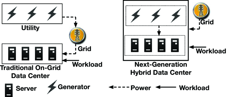
Figure 1: While an “on-grid” data center derives all its power from the grid, next-generation “hybrid” data centers have additional on-site power generation.

data center, there are three time-varying inputs: the server workload $a(t)$ generated by service requests from users and the price of a unit energy from the grid $p(t)$, and the total power consumption function $g_{t}$ for each time $t$ where $1\leq t\leq T$. We begin by investigating offline algorithms that minimize the operating cost with perfect knowledge of the entire input sequence $a(t)$, $p(t)$ and $g_{t}$, for $1\leq t\leq T$. However, in real-life, the time-varying input sequences are not knowable in advance. In particular, the optimization must be performed in an online fashion where decisions at time $t$ are made with the knowledge of inputs $a(\tau)$,$p(\tau)$ and $g_{\tau}$, for $1\leq\tau\leq t+w$, where $w\geq 0$ is a small (possibly zero) look-ahead window. Specifically, an online algorithm has no knowledge of inputs beyond the look-ahead window, i.e., for time $t+w<\tau\leq T$. We assume the inputs within the look-ahead are perfectly known when analyzing the algorithm performance. In practice, short-term demand or grid price can be estimated rather accurately by various techniques including pattern analysis and time series analysis and prediction [19, 14]. As is typical in the study of online algorithms [12], we seek theoretical guarantees for our online algorithms by computing the competitive ratio that is ratio of the cost achieved by the online algorithm for an input to the optimal cost achieved for the same input by an offline algorithm. The competitive ratio is computed under a worst case scenario where an adversary picks the worst possible inputs for the online algorithm. Thus, a small competitive ratio provides a strong guarantee that the online algorithm will achieve a cost close to the offline optimal even for the worst case input.

Our Contributions

A key contribution of our work is to formulate and study data center cost minimization (DCM) that integrates energy procurement from the grid, energy production using on-site generators, and dynamic server capacity management. Our work jointly optimizes the two components of DCM: energy provisioning (EP) from the grid and generators and capacity provisioning (CP) of the servers.

• We theoretically evaluate the benefit of joint optimization by showing that optimizing energy provisioning (EP) and capacity provisioning (CP) separately results in a factor loss of optimality $\rho=LP_{\max}/\left(Lc_{o}+c_{m}\right)$ compared to optimizing them jointly, where $P_{\max}$ is the maximum grid power price, and $L,$ $c_{o,}$ and $c_{m}$ are the capacity, incremental cost, and base cost of an on-site generator respectively. Further, we derive an efficient offline optimal algorithm for hybrid data centers that jointly optimize EP and CP to minimize the data center’s operating cost.

• For on-grid data centers, we devise an online deterministic algorithm that achieves a competitive ratio of $2-\alpha_{s}$, where $\alpha_{s}\in[0,1]$ is the normalized look-ahead window size. Further, we show that our algorithm has the best competitive ratio of any deterministic online algorithm for the problem (c.f. Table 1). For the more complex hybrid data centers, we devise an online deterministic algorithm that achieves a competitive ratio of $\frac{P_{\max}\left(2-\alpha_{s}\right)}{c_{o}+c_{m}/L}\left[1+2\frac{P_{\max}-c_{o}}{P_{\max}(1+\alpha_{g})}\right]$, where $\alpha_{s}$ and $\alpha_{g}$ are normalized look-ahead window sizes. Both online algorithms perform better as the look-ahead window increases, as they are better able to plan their current actions based on knowledge of future inputs. Interestingly, in the on-grid case, we show that there exists fixed threshold value for the look-ahead window for which the online algorithm matches the offline optimal in performance achieving a competitive ratio of 1, i.e., there is no additional benefit gained by the online algorithm if its look-ahead is increased beyond the threshold.

  Competitive	On-grid	Hybrid
  Ratio
  No Look-ahead	2	$\frac{2P_{\max}}{c_{o}+c_{m}/L}\left[1+2\frac{P_{\max}-c_{o}}{P_{\max}}\right]$
  With Look-ahead	$2-\alpha_{s}$	$\frac{P_{\max}\left(2-\alpha_{s}\right)}{c_{o}+c_{m}/L}\left[1+2\frac{P_{\max}-c_{o}}{P_{\max}(1+\alpha_{g})}\right]$

  Table 1: Summary of algorithmic results. The on-grid results are the best possible for any deterministic online algorithm.

• Using extensive workload traces from Akamai and the corresponding grid prices, we simulate our offline and online algorithms in a realistic setting with the goal of empirically evaluating their performance. Our offline optimal (resp., online) algorithm achieves a cost reduction of 25.8% (resp., 20.7%) for a hybrid data center and 12.3% (resp., 7.3%) for an on-grid data center. The cost reduction is computed in comparison with the baseline cost achieved by the current practice of statically provisioning the servers and using only the power grid. The cost reductions are quite significant and make a strong case for utilizing our joint cost optimization framework. Furthermore, our online algorithms obtain almost the same cost reduction as the offline optimal solution even with a small look-ahead of 6 hours, indicating the value of short-term prediction of inputs.

• A hybrid data center provides about 13% additional cost reduction over an on-grid data center representing the additional cost benefits that on-site power generation provides over using the grid alone. Interestingly, it is sufficient to deploy a partial on-site generation capacity that provides 60% of the peak power requirements of the data center to obtain over 95% of the additional cost reduction. This provides strong motivation for a traditional on-grid data center to deploy at least a partial on-site generation capability to save costs.

2 The Data Center Cost Minimization Problem

We consider the scenario where a data center can jointly optimize energy production, procurement, and consumption so as to minimize its operating expenses. We refer to this data center cost minimization problem as DCM. To study DCM, we model how energy is produced using on-site power generators, how it can be procured from the power grid, and how data center capacity can be provisioned dynamically in response to workload. While some of these aspects have been studied independently, our work is unique in optimizing these dimensions simultaneously as next-generation data centers can. Our algorithms minimize cost by use of techniques such as: (i) dynamic capacity provisioning of servers – turning off unnecessary servers when workload is low to reduce the energy consumption (ii) opportunistic energy procurement – opting between the on-site and grid energy sources to exploit price fluctuation, and (iii) dynamic provisioning of generators - orchestrating which generators produce what portion of the energy demand. While prior literature has considered these techniques in isolation, we show how they can be used in coordination to manage both the supply and demand of power to achieve substantial cost reduction.

Notation	Definition
$T$	Number of time slots
$N$	Number of on-site generators
$\beta_{s}$	Switching cost of a server ($)
$\beta_{g}$	Startup cost of an on-site generator ($)
$c_{m}$	Sunk cost of maintaining a generator in its active state per slot ($)
$c_{o}$	Incremental cost for an active generator to output an additional unit of energy ($/Wh)
$L$	The maximum output of a generator (Watt)
$a(t)$	Workload at time $t$
$p(t)$	Price per unit energy drawn from the grid at $t$ ($P_{\min}\leq p(t)\leq P_{\max}$) ($/Wh)
$x(t)$	Number of active servers at $t$
$s(t)$	Total server service capability at $t$
$v(t)$	Grid power used at $t$ (Watt)
$y(t)$	Number of active on-site generators at $t$
$u(t)$	Total power output from active generators at $t$ (Watt)
$g_{t}(x(t),a(t))$	Total power consumption as a function of $x(t)$ and $a(t)$ at $t$ (Watt)

Note: we use bold symbols to denote vectors, e.g., $\boldsymbol{x}=\langle x(t)\rangle$. Brackets indicate the unit.

Table 2: Key notation.

2.1 Model Assumptions

We adopt a discrete-time model whose time slot matches the timescale at which the scheduling decisions can be updated. Without loss of generality, we assume there are totally $T$ slots, and each has a unit length.

Workload model. Similar to existing work [13, 34, 16], we consider a “mice” type of workload for the data center where each job has a small transaction size and short duration. Jobs arriving in a slot get served in the same slot. Workload can be split among active servers at arbitrary granularity like a fluid. These assumptions model a “request-response” type of workload that characterizes serving web content or hosted application services that entail short but real-time interactions between the user and the server. The workload to be served at time $t$ is represented by $a(t)$. Note that we do not rely on any specific stochastic model of $a(t)$.

Server model. We assume that the data center consists of a sufficient number of homogeneous servers, and each has unit service capacity, i.e., it can serve at most one unit workload per slot, and the same power consumption model. Let $x(t)$ be the number of active servers and $s(t)\in[0,x(t)]$ be the total server service capability at time $t$. It is clear that $s(t)$ should be larger than $a(t)$ to get the workload served in the same slot. We model the aggregate server power consumption as $b(t)\triangleq f_{s}\left(x(t),s(t)\right)$, an increasing and convex function of $x(t)$ and $s(t)$. That is, the first and second order partial derivatives in $x(t)$ and $s(t)$ are all non-negative. Since $f_{s}\left(x(t),s(t)\right)$ is increasing in $s(t)$, it is optimal to always set $s(t)=a(t)$. Thus, we have $b(t)=f_{s}\left(x(t),a(t)\right)$ and $x(t)\geq a(t)$.

This power consumption model is quite general and captures many common server models. One example is the commonly adopted standard linear model [9]:

$$f_{s}\left(x(t),a(t)\right)=c_{idle}x(t)+(c_{peak}-c_{idle})a(t),$$

where $c_{idle}$ and $c_{peak}$ are the power consumed by an server at idle and fully utilized state, respectively. Most servers today consume significant amounts of power even when idle. A holy grail for server design is to make them “power proportional” by making $c_{idle}$ zero [32].

Besides, turning a server on entails switching cost [28], denoted as $\beta_{s}$, including the amortized service interruption cost, wear-and-tear cost, e.g., component procurement, replacement cost (hard-disks in particular) and risk associated with server switching. It is comparable to the energy cost of running a server for several hours [23].

In addition to servers, power conditioning and cooling systems also consume a significant portion of power. The three contribute about 94% of overall power consumption and their power draw vary drastically with server utilization [33]. Thus, it is important to model the power consumed by power conditioning and cooling systems.

Power conditioning system model. Power conditioning system usually includes power distribution units (PDUs) and uninterruptible power supplies (UPSs). PDUs transform the high voltage power distributed throughout the data center to voltage levels appropriate for servers. UPSs provides temporary power during outage. We model the power consumption of this system as $f_{p}(b(t))$, an increasing and convex function of the aggregate server power consumption $b(t)$.

This model is general and one example is a quadratic function adopted in a comprehensive study on the data center power consumption [33]: $f_{p}(b(t))=C_{1}+\pi_{1}b^{2}(t)$, where $C_{1}>0$ and $\pi_{1}>0$ are constants depending on specific PDUs and UPSs.

Cooling system model. We model the power consumed by the cooling system as $f_{c}^{t}(b(t))$, a time-dependent (e.g., depends on ambient weather conditions) increasing and convex function of $b(t)$.

This cooling model captures many common cooling systems. According to [24], the power consumption of an outside air cooling system can be modelled as a time-dependent cubic function of $b(t)$: $f_{c}^{t}(b(t))=K_{t}b^{3}(t),$ where $K_{t}>0$ depends on ambient weather conditions, such as air temperature, at time $t$. According to [33], the power draw of a water chiller cooling system can be modelled as a time-dependent quadratic function of $b(t)$: $f_{c}^{t}(b(t))=Q_{t}b^{2}(t)+L_{t}b(t)+C_{t},$ where $Q_{t},L_{t},C_{t}\geq 0$ depend on outside air and chilled water temperature at time $t$. Note that all we need is $f_{c}^{t}(b(t))$ is increasing and convex in $b(t)$.

On-site generator model. We assume that the data center has $N$ units of homogeneous on-site generators, each having an power output capacity $L$. Similar to generator models studied in the unit commitment problem [20], we define a generator startup cost $\beta_{g}$, which typically involves heating up cost, additional maintenance cost due to each startup (e.g., fatigue and possible permanent damage resulted by stresses during startups), $c_{m}$ as the sunk cost of maintaining a generator in its active state for a slot, and $c_{o}$ as the incremental cost for an active generator to output an additional unit of energy. Thus, the total cost for $y(t)$ active generators that output $u(t)$ units of energy at time $t$ is $c_{m}y(t)+c_{o}u(t)$.

Grid model. The grid supplies energy to the data center in an “on-demand” fashion, with time-varying price $p(t)$ per unit energy at time $t$. Thus, the cost of drawing $v(t)$ units of energy from the grid at time $t$ is $p(t)v(t)$. Without loss of generality, we assume $0\leq P_{\min}\leq p(t)\leq P_{\max}$.

To keep the study interesting and practically relevant, we make the following assumptions: (i) the server and generator turning-on cost are strictly positive, i.e., $\beta_{s}>0$ and $\beta_{g}>0$. (ii) $c_{o}+c_{m}/L<P_{\max}.$ This ensures that the minimum on-site energy price is cheaper than the maximum grid energy price. Otherwise, it should be clear that it is optimal to always buy energy from the grid, because in that case the grid energy is cheaper and incurs no startup costs.

2.2 Problem Formulation

Based on the above models, the data center total power consumption is the sum of the server, power conditioning system and the cooling system power draw, which can be expressed as a time-dependent function of $b(t)$ ($b(t)=f_{s}(x(t),a(t))$ ):

$$b(t)+f_{p}(b(t))+f_{c}^{t}(b(t))\triangleq g_{t}(x(t),a(t)).$$

We remark that $g_{t}(x(t),a(t))$ is increasing and convex in $x(t)$ and $a(t)$. This is because it is the sum of three increasing and convex functions. Note that all results we derive in this paper apply to any $g_{t}(x,a)$ as long as it is increasing and convex in $x$ and $a$.

Our objective is to minimize the data center total cost in entire horizon $[1,T]$, which is given by

$$\mbox{Cost}(x,y,u,v)\triangleq\sum_{t=1}^{T}\left\{v(t)p(t)+c_{o}u(t)+c_{m}y(t)\right.$$ (1)

$$\qquad\left.+\beta_{s}[x(t)-x(t-1)]^{+}+\beta_{g}[y(t)-y(t-1)]^{+}\right\},$$

which includes the cost of grid electricity, the running cost of on-site generators, and the switching cost of servers and on-site generators in the entire horizon $[1,T]$. Throughout this paper, we set initial condition $x(0)=y(0)=0.$

We formally define the data center cost minimization problem as a non-linear mixed-integer program, given the workload $a(t)$, the grid price $p(t)$ and the time-dependent function $g_{t}(x,a),$ for $1\leq t\leq T$, as time-varying inputs.

$$\min_{x,y,u,v} \mbox{Cost}(x,y,u,v)$$ (2)

s.t. $$u(t)+v(t)\geq g_{t}(x(t),a(t)),$$ (7)

$$u(t)\leq Ly(t),$$

$$x(t)\geq a(t),$$

$$y(t)\leq N,$$

$$x(0)=y(0)=0,$$

var $$x(t),y(t)\in\mathbb{N}^{0},u(t),v(t)\in\mathbb{R}_{0}^{+},\,t\in[1,T],$$

where $\left[\cdot\right]^{+}=\max(0,\cdot)$, $\mathbb{N}^{0}$ and $\mathbb{R}_{0}^{+}$ represent the set of non-negative integers and real numbers, respectively.

Constraint (7) ensures the total power consumed by the data center is jointly supplied by the generators and the grid. Constraint (7) captures the maximal output of the on-site generator. Constraint (7) specifies that there are enough active servers to serve the workload. Constraint (7) is generator number constraint. Constraint (7) is the boundary condition.

Note that this problem is challenging to solve. First, it is a non-linear mixed-integer optimization problem. Further, the objective function values across different slots are correlated via the switching costs $\beta_{s}[x(t)-x(t-1)]^{+}$ and $\beta_{g}[y(t)-y(t-1)]^{+}$, and thus cannot be decomposed. Finally, to obtain an online solution we do not even know the inputs beyond current slot.

Next, we introduce a proposition to simplify the structure of the problem. Note that if $\left(x(t)\right)_{t=1}^{T}$ and $\left(y(t)\right)_{t=1}^{T}$ are given, the problem in (2)-(7) reduces to a linear program and can be solved independently for each slot. We then obtain the following.

Proposition 1

Given any $x(t)$ and $y(t)$, the $u(t)$ and $v(t)$ that minimize the cost in (2) with any $g_{t}(x,a)$ that is increasing in x and a, are given by: $\forall t\in[1,T]$,

$$u(t)=\begin{cases}0,&\mbox{if }p(t)\leq c_{o},\\ \min\left(Ly(t),g_{t}(x(t),a(t))\right),&\mbox{otherwise,}\end{cases}$$

and

$$v(t)=g_{t}(x(t),a(t))-u(t).$$

Note that $u(t),v(t)$ can be computed using only $x(t),y(t)$ at current time $t$, thus can be determined in an online fashion.

Intuitively, the above proposition says if the on-site energy price $c_{o}$ is higher than the grid price $p(t)$, we should buy energy from the grid; otherwise, it is the best to buy the cheap on-site energy up to its maximum supply $L\cdot y(t)$ and the rest (if any) from the more expensive grid. With the above proposition, we can reduce the non-linear mixed-integer program in (2)-(7) with variables $\boldsymbol{x}$, $\boldsymbol{y}$, $\boldsymbol{u}$, and $\boldsymbol{v}$ to the following integer program with only variables $\boldsymbol{x}$ and $\boldsymbol{y}$:

$$\mathbf{DCM}:$$

$$\min \sum_{t=1}^{T}\left\{\psi\left(y(t),p(t),d_{t}(x(t))\right)+\beta_{s}[x(t)-x(t-1)]^{+}\right.$$

$$\;\left.+\beta_{g}[y(t)-y(t-1)]^{+}\right\}$$

s.t. $$x(t)\geq a(t),$$

$$\eqref{eq:MP-generator-number-constraint},\eqref{eq:MP-boundary-conditions},$$

var $$x(t),y(t)\in\mathbb{N}^{0},\,t\in[1,T],$$

where $d_{t}(x(t))\triangleq g_{t}(x(t),a(t))$, for the ease of presentation in later sections, is increasing and convex in $x(t)$ and $\psi\left(y(t),p(t),d_{t}(x(t))\right)$ replaces the term $v(t)p(t)+c_{o}u(t)+c_{m}y(t)$ in the original cost function in (2) and is defined as

$$\psi\left(y(t),p(t),d_{t}(x(t))\right)$$

$$\triangleq \begin{cases}c_{m}y(t)+p(t)d_{t}(x(t)),&\mbox{if }p(t)\leq c_{o},\\ c_{m}y(t)+c_{o}Ly(t)+&\mbox{if }p(t)>c_{o}\mbox{ and }\\ p(t)\left(d_{t}(x(t))-Ly(t)\right),&d_{t}(x(t))>Ly(t),\\ c_{m}y(t)+c_{o}d_{t}(x(t)),&\mbox{else.}\end{cases}$$

As a result of the analysis above, it suffices to solve the above formulation of DCM with only variables $\boldsymbol{x}$ and $\boldsymbol{y}$, in order to minimize the data center operating cost.

2.3 An Offline Optimal Algorithm

We present an offline optimal algorithm for solving problem DCM using Dijkstra’s shortest path algorithm [15]. We construct a graph $G=(V,E),$ where each vertex denoted by the tuple $\langle x,y,t\rangle$ represents a state of the data center where there are $x$ active servers, and $y$ active generators at time $t$. We draw a directed edge from each vertex $\langle x(t-1),y(t-1),t-1\rangle$ to each possible vertex $\langle x(t),y(t),t\rangle$ to represent the fact that the data center can transit from the first state to the second state. Further, we associate the cost of that transition shown below as the weight of the edge:

$$\psi\left(y(t),p(t),d_{t}(x(t))\right)+\beta_{s}[x(t)-x(t-1)]^{+}$$

$$+\beta_{g}[y(t)-y(t-1)]^{+}.$$

Next, we find the minimum weighted path from the initial state represented by vertex $\langle 0,0,0\rangle$ to the final state represented by vertex $\langle 0,0,T+1\rangle$ by running Dijkstra’s algorithm on graph $G$. Since the weights represent the transition costs, it is clear that finding the minimum weighted path in $G$ is equivalent to minimizing the total transitional costs. Thus, our offline algorithm provides an optimal solution for problem DCM.

Theorem 1.

The algorithm described above finds an optimal solution to problem DCM in time $O\left(M^{2}N^{2}T\log\left(MNT\right)\right)$, where $T$ is the number of slots, $N$ the number of generators and $M=\max_{1\leq t\leq T}\left\lceil a(t)\right\rceil$.

Proof.

Since the numbers of active servers and generators are at most $M$ and $N$, respectively, and there are $T+2$ time slots, graph $G$ has $O(MNT)$ vertices and $O(M^{2}N^{2}T)$ edges. Thus, the run time of Dijkstra’s algorithm on graph $G$ is $O\left(M^{2}N^{2}T\log\left(MNT\right)\right)$.∎

Remark: In practice, the time-varying input sequences ($p(t)$, $a(t)$ and $g_{t}$) may not be available in advance and hence it may be difficult to apply the above offline algorithm. However, an offline optimal algorithm can serve as a benchmark, using which we can evaluate the performance of online algorithms.

3 The Benefit of Joint Optimization

Data center cost minimization (DCM) entails the joint optimization of both server capacity that determines the energy demand and on-site power generation that determines the energy supply. Now consider the situation where the data center optimizes the energy demand and supply separately.

First, the data center dynamically provisions the server capacity according to the grid power price $p(t)$. More formally, it solves the capacity provisioning problem which we refer to as CP below.

$$\textbf{CP}: \min \sum_{t=1}^{T}\left\{p(t)\cdot d_{t}(x(t))+\beta_{s}[x(t)-x(t-1)]^{+}\right\}$$

s.t. $$x(t)\geq a(t),$$

$$x(0)=0,$$

var $$x(t)\in\mathbb{N}^{0},\,t\in[1,T].$$

Solving problem CP yields $\boldsymbol{\bar{x}}$. Thus, the total power demand at time $t$ given $\bar{x}(t)$ is $d_{t}(\bar{x}(t))$. Note that $d_{t}(\bar{x}(t))$ is not just server power consumption, but also includes consumption of power conditioning and cooling systems, as described in Sec. 2.2.

Second, the data center minimizes the cost of satisfying the power demand due to $d_{t}(\bar{x}(t))$, using both the grid and the on-site generators. Specifically, it solves the energy provisioning problem which we refer to as EP below.

$$\textbf{EP}:$$

$$\min \sum_{t=1}^{T}\left\{\psi\left(y(t),p(t),d_{t}(\bar{x}(t))\right)+\beta_{g}[y(t)-y(t-1)]^{+}\right\}$$

$$y(0)=0,$$

var $$y(t)\in\mathbb{N}^{0},\,t\in[1,T].$$

Let $(\boldsymbol{\bar{x}},\boldsymbol{\bar{y}})$ be the solution obtained by solving CP and EP separately in sequence and $\left(\boldsymbol{x}^{*},\boldsymbol{y}^{*}\right)$ be the solution obtained by solving the joint-optimization DCM. Further, let ${\rm C_{DCM}}(\boldsymbol{x},\boldsymbol{y})$ be the value of the data center’s total cost for solution $(\boldsymbol{x},\boldsymbol{y})$, including both generator and server costs as represented by the objective function (2.2) of problem DCM. The additional benefit of joint optimization over optimizing independently is simply the relationship between ${\rm C_{DCM}}(\boldsymbol{\bar{x}},\boldsymbol{\bar{y}})$ and ${\rm C_{DCM}}\left(\boldsymbol{x}^{*},\boldsymbol{y}^{*}\right)$. It is clear that $(\boldsymbol{\bar{x}},\boldsymbol{\bar{y}})$ obeys all the constraints of DCM and hence is a feasible solution of DCM. Thus, ${\rm C_{DCM}}\left(\boldsymbol{x}^{*},\boldsymbol{y}^{*}\right)\leq{\rm C_{DCM}}(\boldsymbol{\bar{x}},\boldsymbol{\bar{y}}).$ We can measure the factor loss in optimality $\rho$ due to optimizing separately as opposed to optimizing jointly on the worst-case input as follows:

$$\rho\triangleq\max_{\mbox{all inputs}}\frac{{\rm C_{DCM}}(\boldsymbol{\bar{x}},\boldsymbol{\bar{y}})}{{\rm C_{DCM}}\left(\boldsymbol{x}^{*},\boldsymbol{y}^{*}\right)}.$$

The following theorem characterizes the benefit of joint optimization over optimizing independently.

Theorem 2.

The factor loss in optimality $\rho$ by solving the problem CP and EP in sequence as opposed to optimizing jointly is given by $\rho=LP_{\max}/\left(Lc_{o}+c_{m}\right)$ and it is tight.

Proof.

Refer to Appendix F. ∎

The above theorem guarantees that for any time duration $T$, any workload $\boldsymbol{a}$, any grid price $\boldsymbol{p}$ and any function $g_{t}(x,a)$ as long as it is increasing and convex in $x$ and $a$, solving problem DCM by first solving CP then solving EP in sequence yields a solution that is within a factor $LP_{\max}/\left(Lc_{o}+c_{m}\right)$ of solving DCM directly. Further, the ratio is tight in that there exists an input to DCM where the ratio ${\rm C_{DCM}}(\boldsymbol{\bar{x}},\boldsymbol{\bar{y}})/{\rm C_{DCM}}\left(\boldsymbol{x}^{*},\boldsymbol{y}^{*}\right)$ equals $LP_{\max}/\left(Lc_{o}+c_{m}\right).$

The theorem shows in a quantitative way that a larger price discrepancy between the maximum grid price and the on-site power yields a larger gain by optimizing the energy provisioning and capacity provisioning jointly. Over the past decade, utilities have been exposing a greater level of grid price variation to their customers with mechanisms such as time-of-use pricing where grid prices are much more expensive during peak hours than during the off-peak periods. This likely leads to larger price discrepancy between the grid and the on-site power. In that case, our result implies that a joint optimization of power and server resources is likely to yield more benefits to a hybrid data center.

Besides characterizing the benefit of jointly optimizing power and server resources, the decomposition of problem DCM into problems CP and EP provides a key approach for our online algorithm design. Problem DCM has an objective function with mutually-dependent coupled variables $\boldsymbol{x}$ and $\boldsymbol{y}$ indicating the server and generator states, respectively. This coupling (specifically through the function $\psi\left(y(t),p(t),d_{t}(x(t))\right)$ ) makes it difficult to design provably good online algorithms. However, instead of solving problem DCM directly, we devise online algorithms to solve problems CP that involves only server variable $\boldsymbol{x}$ and EP that involves only the generator variables $\boldsymbol{y}$. Combining the online algorithms for CP and EP respectively yields the desired online algorithm for DCM.

4 Online Algorithms for On-Grid Data Centers

We first develop an online algorithm for DCM for an on-grid data center, where there is no on-site power generation, a scenario that captures most data centers today. Since on-grid data center has no on-site power generation, solving DCM for it reduces to solving problem CP described in Sec. 3.

Problems of this kind have been studied in the literature (see e.g., [23, 27]). The difference of our work from [23, 27] is as follows (also summarized in Table 3). From the modelling aspect, we explicitly take into account power consumption of both cooling and power conditioning systems, in addition to servers. From the formulation aspect, we are solving a different optimization problem, i.e., an integer program with convex and increasing objective function. From the theoretical result aspects, we achieve a small competitive ratio of $2-\alpha_{s}$, which quickly decreases to $1$ as look-ahead window $w$ increase.

	Cooling &	Optimization	Competitive
	Power	Type	Ratio
	Conditioning
LCP	No	obj: convex	3
[23]		var: continuous
CSR	No	obj: linear	$2-\alpha_{s}$
[27]		var: integer
GCSR		obj: convex
this	Yes	and increasing	$2-\alpha_{s}$
work		var: integer

Note that $\alpha_{s}$ is the normalized look-ahead window size, whose representations are different under the different settings of [27] and our work.

Table 3: Comparison of the algorithm GCSR proposed in this paper, CSR in [27], and LCP in [23].

Recall that CP takes as input the workload $\boldsymbol{a}$, the grid price $\boldsymbol{p}$ and the time-dependent function $g_{t},\ \forall t$ and outputs the number of active servers $\boldsymbol{x}$. We construct solutions to CP in a divide-and-conquer fashion. We will first decompose the demand $\boldsymbol{a}$ into sub-demands and define corresponding sub-problem for each server, and then solve capacity provisioning separately for each sub-problem. Note that the key is to correctly decompose the demand and define the subproblems so that the combined solution is still optimal. More specifically, we slice the demand as follows: for $1\leq i\leq M=\max_{1\leq t\leq T}\left\lceil a(t)\right\rceil$, $1\leq t\leq T,$

$$a_{i}(t)\triangleq\min\left\{1,\max\left\{0,a(t)-(i-1)\right\}\right\}.$$

And the corresponding sub-problem $\textbf{CP}_{{\rm i}}$ is defined as follows.

$$\textbf{CP}_{{\rm i}}: \min \sum_{t=1}^{T}\left\{p(t)\cdot d_{t}^{i}\cdot x_{i}(t)+\beta_{s}[x_{i}(t)-x_{i}(t-1)]^{+}\right\}$$

s.t. $$x_{i}(t)\geq a_{i}(t),$$

$$x_{i}(0)=0,$$

var $$x_{i}(t)\in\{0,1\},\,t\in[1,T],$$

where $x_{i}(t)$ indicates whether the $i$-th server is on at time $t$ and $d_{t}^{i}\triangleq d_{t}(i)-d_{t}(i-1).$ $d_{t}^{i}$ can be interpreted as the power consumption due to the $i$-th server at $t$.

Problem $\textbf{CP}_{{\rm i}}$ solves the capacity provisioning problem with inputs workload $\boldsymbol{a_{i}}$, grid price $\boldsymbol{p}$ and $d_{t}^{i}$. The key reason for our decomposition is that $\textbf{CP}_{{\rm i}}$ is easier to solve, since $\boldsymbol{a_{i}}$ take values in $[0,1]$ and exactly one server is required to serve each $\boldsymbol{a_{i}}$. Generally speaking, a divide-and-conquer manner may suffer from optimality loss. Surprisingly, as the following theorem states, the individual optimal solutions for problems $\textbf{CP}_{{\rm i}}$ can be put together to form an optimal solution to the original problem CP. Denote ${\rm C_{CP_{i}}}(\boldsymbol{x_{i}})$ as the cost of solution $\boldsymbol{x_{i}}$ for problem $\textbf{CP}_{{\rm i}}$ and ${\rm C_{CP}}(\boldsymbol{x})$ the cost of solution $\boldsymbol{x}$ for problem CP.

Theorem 3.

Consider problem $\mathbf{CP}$ with any $d_{t}(x(t))=g_{t}(x(t),a(t)))$ that is convex in x(t). Let $\bar{\boldsymbol{x}}_{i}$ be an optimal solution and $\boldsymbol{x}_{i}^{on}$ an online solution for problem $\mathbf{CP_{i}}$ with workload $\boldsymbol{a}_{i}$, then $\sum_{i=1}^{M}\bar{\boldsymbol{x}}_{i}$ is an optimal solution for $\mathbf{CP}$ with workload $\boldsymbol{a}$. Furthermore, if $\forall\boldsymbol{a}_{i},i$, we have ${\rm C_{CP_{i}}}(\boldsymbol{x}_{i}^{on})\\ \leq\gamma\cdot{\rm C_{CP_{i}}}(\bar{\boldsymbol{x}}_{i})$ for a constant $\gamma\geq 1$, then ${\rm C_{CP}}(\sum_{i=1}^{M}\boldsymbol{x}_{i}^{on})\leq\gamma\cdot{\rm C_{CP}}(\sum_{i=1}^{M}\bar{\boldsymbol{x}}_{i}),\>\forall\boldsymbol{a}$.

Proof.

Refer to Appendix A. ∎

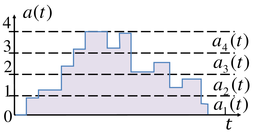
Figure 2: An example of how workload $\boldsymbol{a}$ is decomposed into $4$ sub-demands.

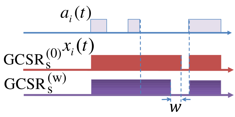
Figure 3: An example of $a_{i}(t)$ and corresponding solution obtained by $\mathbf{GCSR_{s}^{(w)}}$.

Thus, it remains to design algorithms for each $\textbf{CP}_{{\rm i}}$. To solve $\textbf{CP}_{{\rm i}}$ in an online fashion one need only orchestrate one server to satisfy the workload $\boldsymbol{a}_{i}$ and minimize the total cost. When $a_{i}(t)>0$, we must keep the server active to satisfy the workload. The challenging part is what we should do if the server is already active but $a_{i}(t)=0$. Should we turn off the server immediately or keep it idling for some time? Should we distinguish the scenarios when the grid price is high versus low?

Inspired by “ski-rental” [12] and [27], we solve $\textbf{CP}_{{\rm i}}$ by the following “break-even” idea. During the idle period, i.e., $a_{i}(t)=0$, we accumulate an “idling cost” and when it reaches $\beta_{s}$, we turn off the server; otherwise, we keep the server idling. Specifically, our online algorithm $\mathbf{GCSR_{s}^{(w)}}$ (Generalized Collective Server Rental) for $\textbf{CP}_{{\rm i}}$ has a look-ahead window $w$. At time $t$, if there exist $\tau^{\prime}\in[t,t+w]$ such that the idling cost till $\tau^{\prime}$ is at least $\beta_{s}$, we turn off the server; otherwise, we keep it idling. More formally, we have Algorithm 1 and its competitive analysis in Theorem 4. A simple example of $\mathbf{GCSR_{s}^{(w)}}$ is shown in Fig. 3.

Our online algorithm for CP, denoted as $\mathbf{GCSR^{(w)}}$, first employs $\mathbf{GCSR_{s}^{(w)}}$ to solve each $\textbf{CP}_{{\rm i}}$ on workload $\boldsymbol{a}_{i}$, $1\leq i\leq M$, in an online fashion to produce output $\boldsymbol{x}_{i}^{on}$ and then simply outputs $\sum_{i=1}^{M}\boldsymbol{x}_{i}^{on}=\boldsymbol{x}^{on}$ as the output for the original problem CP.

Algorithm 1 $\mathbf{GCSR_{s}^{(w)}}$ for problem $\textbf{CP}_{{\rm i}}$

1:  $C_{i}=0$,$x_{i}(0)=0$

2:  at current time $t,$ do

3:  Set $\tau^{\prime}\leftarrow\min\{t^{\prime}\in[t,t+w]\>|\>C_{i}+\sum_{\tau=t}^{t^{\prime}}p(\tau)d_{\tau}^{i}\geq\beta_{s}\}$

4:  if $a_{i}(t)>0$ then

5:     $x_{i}(t)=1$ and $C_{i}=0$

6:  else if $\tau^{\prime}=\mbox{NULL}$ or $\exists\tau\in[t,\tau^{\prime}]$, $a_{i}(\tau)>0$ then

7:     $x_{i}(t)=x_{i}(t-1)$ and $C_{i}=C_{i}+p(t)d_{t}^{i}x_{i}(t)$

8:  else

9:     $x_{i}(t)=0$ and $C_{i}=0$

10:  end if

Theorem 4.

$\mathbf{GCSR_{s}^{(w)}}$ achieves a competitive ratio of $2-\alpha_{s}$ for $\mathbf{CP_{i}}$, where $\alpha_{s}\triangleq\min\left(1,wd_{\min}P_{\min}/\beta_{s}\right)\in[0,1]$ is a “normalized” look-ahead window size and $d_{\min}\triangleq\min_{t}\{d_{t}(1)\\ -d_{t}(0)\}$. Hence, according to Theorem 3, $\mathbf{GCSR^{(w)}}$ achieves the same competitive ratio for $\mathbf{CP}$. Further, no deterministic online algorithm with a look-ahead window w can achieve a smaller competitive ratio.

Proof.

Refer to Appendix C. ∎

A consequence of Theorem 4 is that when the look-ahead window size $w$ reaches a break-even interval $\Delta_{s}\triangleq\beta_{s}/(d_{\min}P_{\min})$, our online algorithm has a competitive ratio of $1.$ That is, having a look-ahead window larger than $\Delta_{s}$ will not decrease the cost any further.

5 Online Algorithms for Hybrid Data Centers

Unlike on-grid data centers, hybrid data centers have on-site power generation and therefore have to solve both capacity provisioning (CP) and energy provisioning (EP) to solve the data center cost minimization (DCM) problem. We design an online algorithm that we call $\mathbf{DCMON}$ solving DCM as follows.

1. Run algorithm $\mathbf{GCSR}$ from Sec. 4 to solve CP that takes workload $\boldsymbol{a}$, grid price $\boldsymbol{p}$ and time-dependent function $g_{t},\ \forall t$ as input and produces the number of active servers $\boldsymbol{x}^{on}$.

2. Run algorithm $\mathbf{CHASE}$ described in Section 5.2 below to solve EP that takes the energy demand $d_{t}(x^{on}(t))=g_{t}(x^{on}(t),a(t))$ and grid price $p(t),\ \forall t$ as input and decides when to turn on/off on-site generators and how much power to draw from the generators and the grid. Note that a similar problem has been studied in the microgrid scenarios for energy generation scheduling in our previous work [26]. In this paper, we adapt algorithm $\mathbf{CHASE}$ developed in [26] to our data center scenarios to solve EP in an online fashion.

For the sake of completeness, we first briefly present the design behind $\mathbf{CHASE}$ in Sec. 5.1 and the algorithm and its intuitions in Sec. 5.2. Then we present the combined algorithm $\mathbf{DCMON}$ in Sec. 5.3.

5.1 A useful structure of an offline optimal solution of EP

We first reveal an elegant structure of an offline optimal solution and then exploit this structure in the design of our online algorithm $\mathbf{CHASE}$.

5.1.1 Decompose EP into sub-problems ${EP}_{i}$s

For the ease of presentation, we denote $e(t)=d_{t}(x^{on}(t))$. Similar as the decomposition of workload when solving CP, we decompose the energy demand $\boldsymbol{e}$ into $N$ sub-demands and define sub-problem for each generator, then solve energy provisioning separately for each sub-problem, where $N$ is the number of on-site generators. Specifically, for $1\leq i\leq N,\ 1\leq t\leq T$,

$$e_{i}(t)\triangleq\min\left\{L,\max\left\{0,e(t)-(i-1)L\right\}\right\}.$$

The corresponding sub-problem $\textbf{EP}_{{\rm i}}$ is in the same form as EP except that $d_{t}(\bar{x}(t))$ is replaced by $e_{i}(t)$ and $y(t)$ is replaced by $y_{i}(t)\in\{0,1\}$. Using this decomposition, we can solve EP on input $\boldsymbol{e}$ by simultaneously solving simpler problems $\textbf{EP}_{{\rm i}}$ on input $\boldsymbol{e}_{i}$ that only involve a single generator. Theorem 5 shows that the decomposition incurs no optimality loss. Denote ${\rm C_{EP_{i}}}(\boldsymbol{y_{i}})$ as the cost of solution $\boldsymbol{y_{i}}$ for problem $\textbf{EP}_{{\rm i}}$ and ${\rm C_{EP}}(\boldsymbol{y})$ the cost of solution $\boldsymbol{y}$ for problem EP.

Theorem 5.

Let $\boldsymbol{\bar{y}}_{i}$ be an optimal solution and $\boldsymbol{y}_{i}^{on}$ an online solution for $\mathbf{EP_{i}}$ with energy demand $\boldsymbol{e}_{i}$, then $\sum_{i=1}^{N}\boldsymbol{\bar{y}}_{i}$ is an optimal solution for $\mathbf{EP}$ with energy demand $\boldsymbol{e}$. Furthermore, if $\forall\boldsymbol{e}_{i},i$, we have ${\rm C_{EP_{i}}}(\boldsymbol{y}_{i}^{on})\leq\gamma\cdot{\rm C_{EP_{i}}}(\boldsymbol{\bar{y}}_{i})$ for a constant $\gamma\geq 1$, then ${\rm C_{EP}}(\sum_{i=1}^{N}\boldsymbol{y}_{i}^{on})\leq\gamma\cdot{\rm C_{EP}}(\sum_{i=1}^{N}\boldsymbol{\bar{y}}_{i}),\>\forall\boldsymbol{e}$.

Proof.

Refer to Appendix B. ∎

5.1.2 Solve each sub-problem ${EP}_{i}$

Based on Theorem 5, it remains to design algorithms for each $\textbf{EP}_{{\rm i}}$. Define

$$r_{i}(t)=\psi\left(0,p(t),e_{i}(t)\right)-\psi\left(1,p(t),e_{i}(t)\right).$$ (10)

$r_{i}(t)$ can be interpreted as the one-slot cost difference between not using and using on-site generation. Intuitively, if $r_{i}(t)>0$ (resp. $r_{i}(t)<0$), it will be desirable to turn on (resp. off) the generator. However, due to the startup cost, we should not turn on and off the generator too frequently. Instead, we should evaluate whether the cumulative gain or loss in the future can offset the startup cost. This intuition motivates us to define the following cumulative cost difference $R_{i}(t)$. We set initial values as $R_{i}(0)=-\beta_{g}$ and define $R_{i}(t)$ inductively:

$$R_{i}(t)\triangleq\min\left\{0,\max\left\{-\beta_{g},R_{i}(t-1)+r_{i}(t)\right\}\right\},$$ (11)

Note that $R_{i}(t)$ is only within the range $[-\beta_{g},0]$. An important feature of $R_{i}(t)$ useful later in online algorithm design is that it can be computed given the past and current inputs. An illustrating example of $R_{i}(t)$ is shown in Fig. 5.

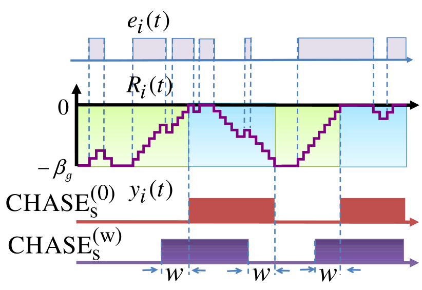
Figure 4: An example of $e_{i}(t)$, $R_{i}(t)$ and the corresponding solution obtained by $\mathbf{CHASE_{s}^{(w)}}$ for $\textbf{EP}_{{\rm i}}$.

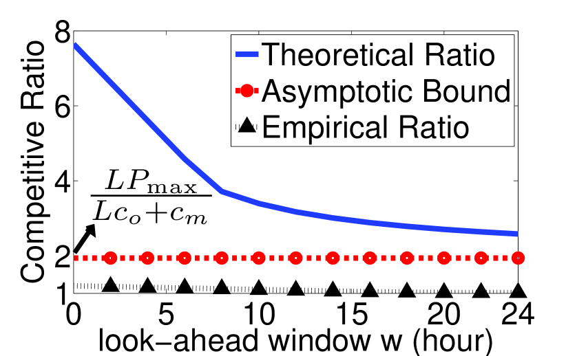
Figure 5: Theoretical and empirical ratios of algorithm $\mathbf{DCMON^{(w)}}$ vs. look-ahead window size w.

Intuitively, when $R_{i}(t)$ hits its boundary $0$, the cost difference between not using and using on-site generation within a certain period is at least $\beta_{g}$, which can offset the startup cost. Thus, it makes sense to turn on the generator. Similarly, when $R_{i}(t)$ hits $-\beta_{g}$, it may be better to turn off the generator and use the grid. The following theorem formalizes this intuition, and shows an optimal solution $\bar{y}_{i}(t)$ for problem $\textbf{EP}_{{\rm i}}$ at the time epoch when $R_{i}(t)$ hits its boundary values $-\beta_{g}$ or $0$.

Theorem 6.

There exists an offline optimal solution for problem $\mathbf{EP_{i}}$ , denoted by $\bar{y}_{i}(t)$, $1\leq t\leq T$, so that:

• if $R_{i}(t)=-\beta_{g}$, then $\bar{y}_{i}(t)=0;$

• if $R_{i}(t)=0$, then $\bar{y}_{i}(t)=1.$

Proof.

Refer to Appendix D. ∎

5.2 Online algorithm CHASE

Our online algorithm $\mathbf{CHASE_{s}^{(w)}}$ with look-ahead window $w$ exploits the insights revealed in Theorem 6 to solve $\textbf{EP}_{{\rm i}}$. The idea behind $\mathbf{CHASE_{s}^{(w)}}$ is to track the offline optimal in an online fashion. In particular, at time $0$, $R_{i}(0)=-\beta_{g}$ and we set $y_{i}(t)=0$. We keep tracking the value of $R_{i}(t)$ at every time slot within the look-ahead window. Once we observe that $R_{i}(t)$ hits values $-\beta_{g}$ or $0$, we set the $y_{i}(t)$ to the optimal solution as Theorem 6 reveals; otherwise, keep $y_{i}(t)=y_{i}(t-1)$ unchanged. More formally, we have Algorithm 2 and its competitive analysis in Theorem 7. An example of $\mathbf{CHASE_{s}^{(w)}}$ is shown in Fig. 5.

The online algorithm for EP, denoted as $\mathbf{CHASE^{(w)}}$, first employs $\mathbf{CHASE_{s}^{(w)}}$ to solve each $\textbf{EP}_{{\rm i}}$ on energy demand $\boldsymbol{e}_{i}$, $1\leq i\leq N$, in an online fashion to produce output $\boldsymbol{y}_{i}^{on}$ and then simply outputs $\sum_{i=1}^{N}\boldsymbol{y}_{i}^{on}$ as the output for the original problem EP.

Algorithm 2 $\mathbf{CHASE_{s}^{(w)}}$ for problem $\textbf{EP}_{{\rm i}}$

1:  at current time $t,$ do

2:  Obtain $\left(R_{i}(\tau)\right)_{\tau=t}^{t+w}$

3:  Set $\tau^{\prime}\leftarrow\min\{\tau\in[t,t+w]\>|\>R_{i}(\tau)=0\ \mbox{or}\ -\beta_{g}\}$

4:  if $\tau^{\prime}=\mbox{NULL}$ then

5:     $y_{i}(t)=y_{i}(t-1)$

6:  else if $R_{i}(\tau^{\prime})=0$ then

7:     $y_{i}(t)=1$

8:  else

9:     $y_{i}(t)=0$

10:  end if

Theorem 7.

$\mathbf{CHASE_{s}^{(w)}}$ for problem $\mathbf{EP_{i}}$ with a look-ahead window $w$ has a competitive ratio of

$$1+\frac{2\beta_{g}\left(LP{}_{\max}-Lc_{o}-c_{m}\right)}{\beta_{g}LP{}_{\max}+wc_{m}P{}_{\max}\left(L-\frac{c_{m}}{P{}_{\max}-c_{o}}\right)}.$$

Hence, according to Theorem 5, $\mathbf{CHASE^{(w)}}$ achieves the same competitive ratio for problem $\mathbf{EP}$.

Proof.

Refer to Appendix E. ∎

5.3 Combining GCSR and CHASE

Our algorithm $\mathbf{DCMON^{(w)}}$ for solving problem DCM with a look-ahead window of $w\geq 0$, i.e., knowing grid prices $p(\tau)$, workload $a(\tau)$ and the function $g_{\tau},1\leq\tau\leq t+w,$ at time $t$, first uses $\mathbf{GCSR}$ from Sec. 4 to solve problem CP and then uses $\mathbf{CHASE}$ in Sec. 5.2 to solve problem EP. An important observation is that the available look-ahead window size for $\mathbf{GCSR}$ to solve CP is $w$, i.e., knows $p(\tau)$, $a(\tau)$ and $g_{\tau}$, $1\leq\tau\leq t+w,$ at time $t$; however, the available look-ahead window size for $\mathbf{CHASE}$ to solve EP is only $\left[w-\Delta_{s}\right]^{+}$, i.e., knows $p(\tau)$ and $e(\tau)=d_{\tau}(x^{on}(\tau))$, $1\leq\tau\leq t+\left[w-\Delta_{s}\right]^{+},$ at time $t$ ($\Delta_{s}$ is the break-even interval defined in Sec. 4).

This is because at time $t,$ $\mathbf{CHASE^{(w)}}$ knows grid prices $p(\tau)$, workload $a(\tau)$ and the function $g_{\tau},1\leq\tau\leq t+w.$ However, not all the energy demands $\left(e(\tau)\right)_{\tau=1}^{t+w}$ are known by $\mathbf{CHASE^{(w)}}$. Because we derive the server state $\boldsymbol{x^{on}}$ by solving problem CP using our online algorithm $\mathbf{GCSR^{(w)}}$ using $p(\tau),\ a(\tau),\ g_{\tau},\ 1\leq\tau\leq t+w.$ A key observation is that at time $t$ it is not possible to compute $\boldsymbol{x^{on}}$ for the full look-ahead window of $t+w,$ since $x^{on}(t+1),\ldots,x^{on}(t+w)$ may depend on inputs $p(\tau),\ a(\tau),\ g_{\tau},\tau>t+w$ that our algorithm does not yet know. Fortunately, for $w\geq\Delta_{s}$ we can determine all $x^{on}(\tau),1\leq\tau\leq t+\left[w-\Delta_{s}\right]^{+}$ given inputs within the full look-ahead window. That is, while we knows the grid prices $p$, the workload $a$ and the function $g_{t}$ for the full look-ahead window $w$, the server state $x^{on}$ is known only for a smaller window of $\left[w-\Delta_{s}\right]^{+}$. Thus, the energy demand $e(\tau)=d_{\tau}(x^{on}(\tau))=g_{\tau}(x^{on}(\tau),a(\tau)),\ 1\leq\tau\leq t+\left[w-\Delta_{s}\right]^{+}$ is available for $\mathbf{CHASE^{(w)}}$ at time $t$.

Thus, a bound on the competitive ratio of $\mathbf{DCMON^{(w)}}$ is the product of competitive ratios for $\mathbf{GCSR^{(w)}}$ and
$\mathbf{CHASE^{(\left[w-\Delta_{s}\right]^{+})}}$ from Theorems 4 and 7, respectively, and the optimality loss ratio $LP_{\max}/\left(Lc_{o}+c_{m}\right)$ due to the offline-decomposition stated in Sec. 3, which is given in the following Theorem.

Theorem 8.

$\mathbf{DCMON^{(w)}}$ for problem DCM has a competitive ratio of

$$\frac{P_{\max}\left(2-\alpha_{s}\right)}{c_{o}+c_{m}/L}\left[1+\frac{2\left(LP{}_{\max}-Lc_{o}-c_{m}\right)}{LP{}_{\max}+\alpha_{g}P{}_{\max}\left(L-\frac{c_{m}}{P{}_{\max}-c_{o}}\right)}\right].$$ (12)

The ratio is also upper-bounded by

$$\frac{P_{\max}\left(2-\alpha_{s}\right)}{c_{o}+c_{m}/L}\left[1+2\frac{P_{\max}-c_{o}}{P_{\max}}\cdot\frac{1}{1+\alpha_{g}}\right],$$

where $\alpha_{s}=\min\left(1,w/\Delta_{s}\right)\in[0,1]$ and $\alpha_{g}\triangleq\frac{c_{m}}{\beta_{g}}\left[w-\Delta_{s}\right]^{+}\\ \in[0,+\infty)$ are “normalized” look-ahead window sizes.

Proof.

Refer to Appendix G. ∎

As the look-ahead window size $w$ increases, the competitive ratio in Theorem 8 decreases to $LP_{\max}/\left(Lc_{o}+c_{m}\right)$ (c.f. Fig. 5), the inherent approximation ratio introduced by our offline decomposition approach discussed in Section 3. However, the real trace based empirical performance of $\mathbf{DCMON^{(w)}}$ without look-ahead is already close to the offline optimal, i.e., ratio close to 1 (c.f. Fig. 5).

6 Empirical Evaluation

We evaluate the performance of our algorithms by simulations based on real-world traces with the aim of (i) corroborating the empirical performance of our online algorithms under various realistic settings and the impact of having look-ahead information, (ii) understanding the benefit of opportunistically procuring energy from both on-site generators and the grid, as compared to the current practice of purchasing from the grid alone, (iii) studying how much on-site energy is needed for substantial cost benefits.

6.1 Parameters and Settings

Workload trace: We use the workload traces from the Akamai network [1, 30] that is the currently the world’s largest content delivery network. The traces measure the workload of Akamai servers serving web content to actual end-users. Note that our workload is of the “request-and-response” type that we model in our paper. We use traces from the Akamai servers deployed in the New York and San Jose data centers that record the hourly average load served by each deployed server over 22 days from Dec. 21, 2008 to Jan. 11, 2009. The New York trace represents 2.5K servers that served about $1.4\times 10^{10}$ requests and $1.7\times 10^{13}$ bytes of content to end-users during our measurement period. The San Jose trace represents 1.5K servers that served about $5.5\times 10^{9}$ requests and $8\times 10^{12}$ bytes of content. We show the workload in Fig. 6, in which we normalize the load by the server’s service capacity. The workload is quite characteristic in that it shows daily variations (peak versus off-peak) and weekly variations (weekday versus weekend).

Grid price: We use traces of hourly grid power prices in New York [2] and San Jose [3] for the same time period, so that it can be matched up with the workload traces (c.f. Fig. 6). Both workload and grid price traces show strong diurnal properties: in the daytime, the workload and the grid price are relatively high; at night, on the contrary, both are low. This indicates the feasibility of reducing the data center cost by using the energy from the on-site generators during the daytime and use the grid at night.

Server model: As mentioned in Sec. 2, we assume the data center has a sufficient number of homogeneous servers to serve the incoming workload at any given time. Similar to a typical setting in [32], we use the standard linear server power consumption model. We assume that each server consumes 0.25KWh power per hour at full capacity and has a power proportional factor (PPF=$(c_{peak}-c_{idle})/c_{peak}$) of 0.6, which gives us $c_{idle}=0.1KW$, $c_{peak}=0.25KW$. In addition, we assume the server switching cost equals the energy cost of running a server for 3 hours. If we assume an average grid price as the price of energy, we get about $\beta_{s}=\$0.08$.

Cooling and power conditioning system model: We consider a water chiller cooling system. According to [5], during this 22-day winter period the average high and low temperatures of New York are $41^{\circ}F$ and $29^{\circ}F$, respectively. Those of San Jose are $58^{\circ}F$ and $41^{\circ}F$, respectively. Without loss of generality, we take the high temperature as the daytime temperature and the low temperature as the nighttime temperature. Thus, according to [33], the power consumed by water chiller cooling systems of the New York and San Jose data centers are about

$$f_{c,NY}^{t}(b)=\begin{cases}(0.041b^{2}+0.144b+0.047)b_{\max},&\mbox{at daytime},\\ (0.03b^{2}+0.136b+0.042)b_{\max},&\mbox{at nighttime},\end{cases}$$

and

$$f_{c,SJ}^{t}(b)=\begin{cases}(0.06b^{2}+0.16b+0.054)b_{\max},&\mbox{at daytime},\\ (0.041b^{2}+0.144b+0.047)b_{\max},&\mbox{at nighttime},\end{cases}$$

where $b_{\max}$ is the maximum server power consumption and $b$ is the server power consumption normalized by $b_{\max}$. The maximum server power consumption of the New York and San Jose data centers are $b_{\max}^{NY}=2500\times 0.25=625KW$ and $b_{\max}^{SJ}=1500\times 0.25=375KW$. Besides, the power consumed by the power conditioning system, including PDUs and UPSs, is $f_{p}(b)=(0.012b^{2}+0.046b+0.056)b_{\max}$ [33].

Generator model: We adopt generators with specifications the same as the one in [4]. The maximum output of the generator is 60KW, i.e., $L=60KW$. The incremental cost to generate an additional unit of energy $c_{o}$ is set to be $0.08/KWh, which is calculated according to the gas price [2] and the generator efficiency [4]. Similar to [37], we set the sunk cost of running the generator for unit time $c_{m}=\$1.2$ and the startup cost $\beta_{g}$ equivalent to the amortized capital cost, which gives $\beta_{g}=\$24$. Besides, we assume the number of generators $N=10$, which is enough to satisfy all the energy demand for this trace and model we use.

Cost benchmark: Current data centers usually do not use dynamic capacity provisioning and on-site generators. Thus, we use the cost incurred by static capacity provisioning with grid power as the benchmark using which we evaluate the cost reduction due to our algorithms. Static capacity provisioning runs a fixed number of servers at all times to serve the workload, without dynamically turning on/off the servers. For our benchmark, we assume that the data center has complete workload information ahead of time and provisions exactly to satisfy the peak workload and uses only grid power. Using such a benchmark gives us a conservative evaluation of the cost saving from our algorithms.

Comparisons of Algorithms: We compare four algorithms: our online and offline optimal algorithms in on-grid scenarios, i.e., $\mathbf{GCSR}$ and $\mathbf{CPOFF}$, and hybrid scenarios, i.e., $\mathbf{DCMON}$ and $\mathbf{DCMOFF}$.

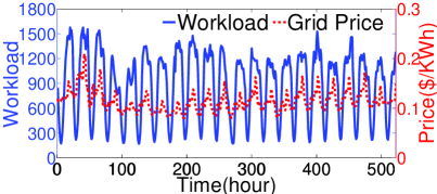
(a) New York

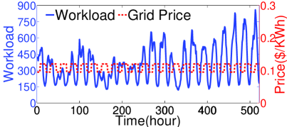
(b) San Jose

Figure 6: Real-world workload from Akamai and the grid power price.

6.2 Impact of Model Parameters on Cost Reduction

We study the cost reduction provided by our offline and online algorithms for both on-grid and hybrid data centers using the New York trace unless specified otherwise. We assume no look-ahead information is available when running the online algorithms. We compute the cost reduction (in percentage) as compared to the cost benchmark which we described earlier. When all parameters take their default values, our offline (resp. online) algorithms provide up to 12.3% (resp., 7.3%) cost reduction for on-grid and 25.8% (resp., 20.7%) cost reduction for hybrid data centers (c.f. Fig. 7. The default value of $c_{o}$ is $0.08/KWh.). Note that the online algorithms provide cost reduction that are 5% smaller than offline algorithms on account of their lack of knowledge of future inputs. Further, note that cost reduction of a hybrid data center is larger than that of a on-grid data center, since hybrid data center has the ability to generate energy on-site to avoid higher grid prices. Nevertheless, the extent of cost reduction in all cases is high providing strong evidence for the need to perform energy and server capacity optimizations.

Data centers may deploy different types of servers and generators with different model parameters. It is then important to understand the impact on cost reduction due to these parameters. We first study the impact of varying $c_{o}$ (c.f. Fig. 7). For a hybrid data center, as $c_{o}$ increases the cost of on-site generation increases making it less effective for cost reduction (c.f Fig. 7a). For the same reason, the cost reduction of a hybrid data center tends to that of the on-grid data center with increasing $c_{o}$ as on-site generation becomes less economical.

We then study the impact of power proportional factor (PPF). More specifically, we fix $c_{peak}=0.25KW$, and vary PPF from 0 to 1 (c.f. Fig. 7b). As PPF increases, the server idle power decreases, thus dynamic provisioning has lesser impact on the cost reduction. This explains why CP achieves no cost reduction when PPF=1. Since DCM also solves CP problem, its performance degrades with increasing PPF as well.

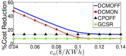
(a) Cost Reduction vs. $c_{o}$

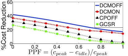
(b) Cost Reduction vs. PPF

Figure 7: Variation of cost reduction with model parameters.

6.3 The Relative Value of Energy versus Capacity Provisioning

In this subsection, we use both New York and San Jose traces. For a hybrid data center, we ask which optimization provides a larger cost reduction: energy provisioning (EP) or server capacity provisioning (CP) in comparison with the joint optimization of doing both (DCM). The cost reductions of different optimization are shown in Fig. 8.

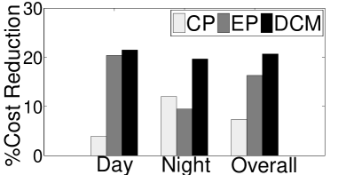
(a) New York

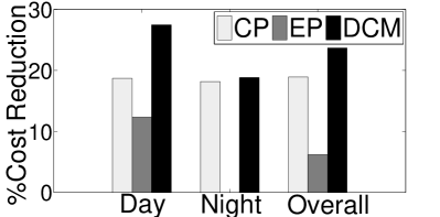
(b) San Jose

Figure 8: Relative values of CP, EP, and DCM.

For the New York scenario in Fig. 8a, overall, we see that EP, CP, and DCM provide cost reductions of 16.3%, 7.3%, and 20.7%, respectively. However, note that during the day doing EP alone provides almost as much cost reduction as the joint optimization DCM. The reason is that during the high traffic hours in the day, solving EP to avoid higher grid prices provides a larger benefit than optimizing the energy consumption by server shutdown. The opposite is true during the night where CP is more critical than EP, since minimizing the energy consumption by shutting down idle servers yields more benefit.

For the San Jose scenario in Fig. 8b, overall, EP, CP, and DCM provide cost reductions of 6.1%, 19%, and 23.7%, respectively. Compared to the New York scenario, the reason why EP achieves so little cost reduction is that the grid power is cheaper and thus on-site generation is not that economical. Meanwhile, CP performs closer to DCM, which is because the workload curve is highly skew (shown in Fig. 6b) and dynamic provisioning for the server capacity saves a lot of server idling cost as well as cooling and power conditioning cost.

In a nutshell, EP favors high grid power price while workload with less regular pattern makes CP more competitive.

6.4 Benefit of Looking Ahead

We evaluate the cost reduction benefit of increasing the look-ahead window. From Fig. 9a, we observe that while the performance of our online algorithms are already good when there is no look-ahead information, they quickly improve to the offline optimal when a small amount of look-ahead, e.g., 6 hours, is available, indicating the value of short-term prediction of inputs. Note that while the competitive ratio analysis in Theorem 8 is for the worst case inputs, our online algorithms perform much closer to the offline optimal for realistic inputs.

6.5 How Much On-site Power Production is Enough

Thus far, in our experiments, we assumed that a hybrid data center had the ability to supply all its energy from on-site power generation ($N=10$). However, an important question is how much investment should a data center operator make in installing on-site generator capacity to obtain largest cost reduction.

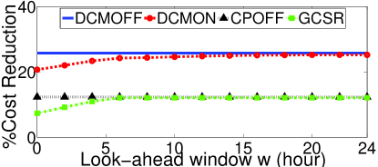
(a) Cost Reduction vs. look-ahead window size w

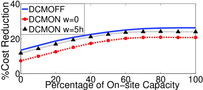
(b) Cost Reduction vs. percentage of on-site power production capacity

Figure 9: Variation of cost reduction with look-ahead and on-site capacity.

More specifically, we vary the number of on-site generators $N$ from 0 to 10 and show the corresponding performances of our algorithms. Interestingly, in Fig. 9b, our results show that provisioning on-site generators to produce 80% of the peak power demand of the data center is sufficient to obtain all of the cost reduction benefits. Further, with just 60% on-site power generation capacity we can achieve 95% of the maximum cost reduction. The intuitive reason is that most of time the demands of the data center are significantly lower than their peaks.

7 Related Work

Our study is among a series of work on dynamic provisioning in data centers and power systems [38, 22, 35].

In particular, for the capacity provisioning problem, [23] and [27] propose online algorithms with performance guarantee to reduce servers operating cost under convex and linear mixed integer optimization scenarios, respectively. Different from these two, our work designs online algorithm under non-linear mixed integer optimization scenario and we take into account the operating cost of servers as well as power conditioning and cooling systems. [24, 39] also model cooling systems, but focus on offline optimization of the operating cost.

Energy provisioning for power systems is characterized by unit-commitment problem (UC) [8, 31], including a mixed-integer programming approach [29] approach and a stochastic control approach [36]. All these approaches assume the demand (or its distribution) in the entire horizon is known a priori, thus they are applicable only when future input information can be predicted with certain level of accuracy. In contrast, in this paper we consider an online setting where the algorithms may utilize only information in the current time slot.

In addition to the difference of our work and existing works in the two problems (i.e., capacity provisioning and energy provisioning), our work is also unique in that we jointly optimize both problems while existing works focus on only one of them.

8 Conclusions

Our work focuses on the cost minimization of data centers achieved by jointly optimizing both the supply of energy from on-site power generators and the grid, and the demand for energy from its deployed servers as well as power conditioning and cooling systems. We show that such an integrated approach is not only possible in next-generation data centers but also desirable for achieving significant cost reductions. Our offline optimal algorithm and our online algorithms with provably good competitive ratios provide key ideas on how to coordinate energy procurement and production with the energy consumption. Our empirical work answers several of the important questions relevant to data center operators focusing on minimizing their operating costs. We show that a hybrid (resp., on-grid) data center can achieve a cost reduction between 20.7% to 25.8% (resp., 7.3% to 12.3%) by employing our joint optimization framework. We also show that on-site power generation can provide an additional cost reduction of about 13%, and that most of the additional benefit is obtained by a partial on-site generation capacity of 60% of the peak power requirement of the data center.

This work can be extended in several directions. First, it is interesting to study how energy storage devices can be used to further reduce the data center operating cost. Second, another interesting direction is to generalize our analysis to take into account deferable workloads. Third, extension from homogeneous servers and generators to heterogeneous setting is also of great interest.

9 Acknowledgments

The work described in this paper was partially supported by China National 973 projects (No. 2012CB315904 and 2013CB336700), several grants from the University Grants Committee of the Hong Kong Special Administrative Region, China (Area of Excellence Project No. AoE/E-02/08 and General Research Fund Project No. 411010 and 411011), and two gift grants from Microsoft and Cisco.

Appendix A Proof of Theorem 3

First, we show that the combined solution $\sum_{i=1}^{M}\bar{\boldsymbol{x}}_{i}$ is optimal to CP.

Denote ${\rm C_{CP}}(\boldsymbol{x})$ to be cost of CP of solution $\boldsymbol{x}$. Suppose that $\tilde{\boldsymbol{x}}$ is an optimal solution for CP. We will show that we can construct a new feasible solution $\sum_{i=1}^{M}\boldsymbol{\hat{x}}_{i}$ for CP, and a new feasible solution $\boldsymbol{\hat{x}}_{i}$ for each $\textbf{CP}_{{\rm i}}$, such that

$${\rm C_{CP}}(\tilde{\boldsymbol{x}})={\rm C_{CP}}(\sum_{i=1}^{M}\boldsymbol{\hat{x}}_{i})=\sum_{i=1}^{M}{\rm C_{CP_{i}}}(\boldsymbol{\hat{x}}_{i})+\sum_{t=1}^{T}p(t)d_{t}(0).$$ (13)

$\bar{\boldsymbol{x}}_{i}$ is an optimal solution for each $\textbf{CP}_{{\rm i}}$. Hence, ${\rm C_{CP_{i}}}(\boldsymbol{\hat{x}}_{i})\geq{\rm C_{CP_{i}}}(\bar{\boldsymbol{x}}_{i})$ for each $i$. Thus,

$${\rm C_{CP}}(\tilde{\boldsymbol{x}}) = \sum_{i=1}^{M}{\rm C_{CP_{i}}}(\boldsymbol{\hat{x}}_{i})+\sum_{t=1}^{T}p(t)d_{t}(0)$$ (14)

$$\geq \sum_{i=1}^{M}{\rm{\rm C_{CP_{i}}}}(\bar{\boldsymbol{x}}_{i})+\sum_{t=1}^{T}p(t)d_{t}(0).$$

Besides, we also can prove that

$$\sum_{i=1}^{M}{\rm{\rm C_{CP_{i}}}}(\bar{\boldsymbol{x}}_{i})+\sum_{t=1}^{T}p(t)d_{t}(0) \geq {\rm C_{CP}}(\sum_{i=1}^{M}\bar{\boldsymbol{x}}_{i}).$$ (15)

Hence, ${\rm C_{CP}}(\tilde{\boldsymbol{x}})={\rm C_{CP}}(\sum_{i=1}^{M}\bar{\boldsymbol{x}}_{i})$, i.e., $\sum_{i=1}^{M}\bar{\boldsymbol{x}}_{i}$ is an optimal solution for CP.

Then, we show ${\rm C_{CP}}(\sum_{i=1}^{M}\boldsymbol{x}_{i}^{on})\leq\gamma\cdot{\rm C_{CP}}(\sum_{i=1}^{M}\bar{\boldsymbol{x}}_{i})$.

Because ${\rm C_{CP_{i}}}(\boldsymbol{x}_{i}^{on})\leq\gamma\cdot{\rm C_{CP_{i}}}(\bar{\boldsymbol{x}}_{i})$ and $\bar{\boldsymbol{x}}_{i}$ is for $\textbf{CP}_{{\rm i}}$, we have $\gamma\geq 1$. According to Eqn. (14), we obtain

$$\gamma\cdot{\rm C_{CP}}(\tilde{\boldsymbol{x}}) \geq \sum_{i=1}^{M}{\rm C_{CP_{i}}}(\boldsymbol{x}_{i}^{on})+\sum_{t=1}^{T}p(t)d_{t}(0).$$

Besides, we also can prove that

$$\sum_{i=1}^{M}{\rm{\rm C_{CP_{i}}}}(\boldsymbol{x}_{i}^{on})+\sum_{t=1}^{T}p(t)d_{t}(0) \geq {\rm C_{CP}}(\sum_{i=1}^{M}\boldsymbol{x}_{i}^{on}).$$ (16)

Hence, ${\rm C_{CP}}(\sum_{i=1}^{M}\boldsymbol{x}_{i}^{on})\leq\gamma\cdot{\rm C_{CP}}(\sum_{i=1}^{M}\bar{\boldsymbol{x}}_{i})$.

It remains to prove Eqns. (13), (15) and (16), which we show in Lemmas 1 and 2.

Lemma 1

${\rm C_{CP}}(\tilde{\boldsymbol{x}})={\rm C_{CP}}(\sum_{i=1}^{M}\boldsymbol{\hat{x}}_{i})=\sum_{i=1}^{M}{\rm C_{CP_{i}}}(\boldsymbol{\hat{x}}_{i})+\sum_{t=1}^{T}p(t)d_{t}(0).$

Proof.

Define $\boldsymbol{\hat{x}}_{i}$ based on $\tilde{\boldsymbol{x}}$ by:

$$\widehat{x}_{i}(t)=\begin{cases}1,&\mbox{if\ }i\leq\tilde{x}(t)\\ 0,&\mbox{otherwise.}\end{cases}$$

It is straightforward to see that

$$\tilde{x}(t)=\sum_{i=1}^{M}\hat{x}_{i}(t)$$

and $\boldsymbol{\hat{x}}_{i}$ is a feasible solution for $\textbf{CP}_{{\rm i}}$, i.e., $\boldsymbol{\hat{x}}_{i}\geq\boldsymbol{a}_{i}$.

So we have ${\rm C_{CP}}(\tilde{\boldsymbol{x}})={\rm C_{CP}}(\sum_{i=1}^{M}\boldsymbol{\hat{x}}_{i}).$

Note that $\widehat{x}_{1}(t)\geq...\geq\widehat{x}_{M}(t)$ is a decreasing sequence. Because $\widehat{x}_{i}(t)\in\{0,1\},\ \forall i,t$, we obtain

$$\sum_{i=1}^{M}[\hat{x}_{i}(t)-\hat{x}_{i}(t-1)]^{+}$$ (17)

$$= \begin{cases}0,\mbox{\qquad\quad if\ }\sum_{i=1}^{M}\hat{x}_{i}(t)\leq\sum_{i=1}^{M}\hat{x}_{i}(t-1)\\ \sum_{i=1}^{M}\hat{x}_{i}(t)-\sum_{i=1}^{M}\hat{x}_{i}(t-1),\mbox{\ \ \ otherwise }\end{cases}$$

$$= \Big{[}\sum_{i=1}^{M}\hat{x}_{i}(t)-\sum_{i=1}^{M}\hat{x}_{i}(t-1)\Big{]}^{+},$$

and

$$\sum_{i=1}^{M}d_{t}^{i}\cdot\hat{x}_{i}(t)+d_{t}(0) = \sum_{i=1}^{\tilde{x}(t)}d_{t}^{i}\cdot 1+d_{t}(0)$$ (18)

$$= \sum_{i=1}^{\tilde{x}(t)}\left[d_{t}(i)-d_{t}(i-1)\right]+d_{t}(0)$$

$$= d_{t}(\tilde{x}(t))-d_{t}(0)+d_{t}(0)$$

$$= d_{t}(\tilde{x}(t))=d_{t}(\sum_{i=1}^{M}\hat{x}_{i}(t)).$$

By Eqns. (17) and (18),

$${\rm C_{CP}}(\sum_{i=1}^{M}\boldsymbol{\hat{x}}_{i})=\sum_{i=1}^{M}{\rm C_{CP_{i}}}(\boldsymbol{\hat{x}}_{i})+\sum_{t=1}^{T}p(t)d_{t}(0).$$

This completes the proof of this lemma.∎

Lemma 2

$\sum_{i=1}^{M}{\rm{\rm C_{CP_{i}}}}(\boldsymbol{x}_{i})+\sum_{t=1}^{T}p(t)d_{t}(0)\geq{\rm C_{CP}}(\sum_{i=1}^{M}\boldsymbol{x}_{i})$, where $\boldsymbol{x}_{i}$ is any feasible solution for problem $\textbf{CP}_{{\rm i}}$.

Proof.

First, it is straightforward that

$$\sum_{i=1}^{M}[x_{i}(t)-x_{i}(t-1)]^{+}\geq\Big{[}\sum_{i=1}^{M}x_{i}(t)-\sum_{i=1}^{M}x_{i}(t-1)\Big{]}^{+}.$$ (19)

Denote $x(t)=\sum_{i=1}^{M}x_{i}(t)$. Then, $\forall t$,

$$\sum_{i=1}^{M}d_{t}^{i}\cdot x_{i}(t)+d_{t}(0) \geq \sum_{i=1}^{x(t)}d_{t}^{i}+d_{t}(0)$$ (20)

$$= d_{t}(x(t))-d_{t}(0)+d_{t}(0)$$

$$= d_{t}(x(t))=d_{t}(\sum_{i=1}^{M}x_{i}(t)),$$

where the first inequality comes from $x_{i}(t)\in\{0,1\}$ and $d_{t}^{1}\leq d_{t}^{2}\leq\cdots\leq d_{t}^{M}$. This is because $d_{t}^{i}=d_{t}(i)-d_{t}(i-1)$ and $d_{t}(x)$ is convex in $x$.

This lemma follows from Eqns. (19) and (20). ∎

Appendix B Proof of Theorem 5

First, we show that the combined solution $\sum_{i=1}^{N}\bar{\boldsymbol{y}}_{i}$ is optimal to EP.

Denote ${\rm C_{EP}}(\boldsymbol{y})$ to be cost of EP of solution $\boldsymbol{y}$. Suppose that $\tilde{\boldsymbol{y}}$ is an optimal solution for EP. We will show that we can construct a new feasible solution $\sum_{i=1}^{N}\boldsymbol{\hat{y}}_{i}$ for EP, and a new feasible solution $\boldsymbol{\hat{y}}_{i}$ for each $\textbf{EP}_{{\rm i}}$, such that

$${\rm C_{EP}}(\tilde{\boldsymbol{y}})={\rm C_{EP}}(\sum_{i=1}^{N}\boldsymbol{\hat{y}}_{i})=\sum_{i=1}^{N}{\rm C_{EP_{i}}}(\boldsymbol{\hat{y}}_{i})+\sum_{t=1}^{T}p(t)\left[e(t)-NL\right]^{+}.$$ (21)

$\boldsymbol{\bar{y}}_{i}$ is an optimal solution for each $\textbf{EP}_{{\rm i}}$. Hence, ${\rm C_{EP_{i}}}(\boldsymbol{\hat{y}}_{i})\geq{\rm C_{EP_{i}}}(\boldsymbol{\bar{y}}_{i})$ for each $i$. Thus,

$${\rm C_{EP}}(\tilde{\boldsymbol{y}}) = \sum_{i=1}^{N}{\rm C_{EP_{i}}}(\boldsymbol{\hat{y}}_{i})+\sum_{t=1}^{T}p(t)\left[e(t)-NL\right]^{+}$$ (22)

$$\geq \sum_{i=1}^{N}{\rm{\rm C_{EP_{i}}}}(\boldsymbol{\bar{y}}_{i})+\sum_{t=1}^{T}p(t)\left[e(t)-NL\right]^{+}.$$

Besides, we also can prove that

$$\sum_{i=1}^{N}{\rm{\rm C_{EP_{i}}}}(\boldsymbol{\bar{y}}_{i})+\sum_{t=1}^{T}p(t)\left[e(t)-NL\right]^{+}\geq{\rm C_{EP}}(\sum_{i=1}^{N}\boldsymbol{\bar{y}}_{i}).$$ (23)

Hence, ${\rm C_{EP}}(\tilde{\boldsymbol{y}})={\rm C_{EP}}(\sum_{i=1}^{N}\boldsymbol{\bar{y}}_{i})$, i.e., $\sum_{i=1}^{N}\boldsymbol{\bar{y}}_{i}$ is an optimal solution for EP.

Then, we show ${\rm C_{EP}}(\sum_{i=1}^{N}\boldsymbol{y}_{i}^{on})\leq\gamma\cdot{\rm C_{EP}}(\sum_{i=1}^{N}\bar{\boldsymbol{y}}_{i})$.

Because ${\rm C_{EP_{i}}}(\boldsymbol{y}_{i}^{on})\leq\gamma\cdot{\rm C_{EP_{i}}}(\bar{\boldsymbol{y}}_{i})$ and $\bar{\boldsymbol{y}}_{i}$ is optimal for $\textbf{EP}_{{\rm i}}$, we have $\gamma\geq 1$. According to Eqn. (22), we have

$$\gamma\cdot{\rm C_{EP}}(\tilde{\boldsymbol{y}}) \geq \sum_{i=1}^{N}{\rm{\rm C_{EP_{i}}}}(\boldsymbol{y}_{i}^{on})+\sum_{t=1}^{T}p(t)\left[e(t)-NL\right]^{+}.$$

Besides, we also can prove that

$$\sum_{i=1}^{N}{\rm{\rm C_{EP_{i}}}}(\boldsymbol{y}_{i}^{on})+\sum_{t=1}^{T}p(t)\left[e(t)-NL\right]^{+}\geq{\rm C_{EP}}(\sum_{i=1}^{N}\boldsymbol{y}_{i}^{on}).$$ (24)

Hence, ${\rm C_{EP}}(\sum_{i=1}^{N}\boldsymbol{y}_{i}^{on})\leq\gamma\cdot{\rm C_{EP}}(\sum_{i=1}^{N}\bar{\boldsymbol{y}}_{i})$.

It remains to prove Eqn. (21), (23) and (24), which we show in Lemmas 3 and 4.

Lemma 3

${\rm C_{EP}}(\tilde{\boldsymbol{y}})={\rm C_{EP}}(\sum_{i=1}^{N}\boldsymbol{\hat{y}}_{i})=\sum_{i=1}^{N}{\rm C_{EP_{i}}}(\boldsymbol{\hat{y}}_{i})+\sum_{t=1}^{T}p(t)\left[e(t)-NL\right]^{+}$.

Proof.

Define $\boldsymbol{\hat{y}}_{i}$ based on $\tilde{\boldsymbol{y}}$ by:

$$\widehat{y}_{i}(t)=\begin{cases}1,&\mbox{if\ }i\leq\tilde{y}(t)\\ 0,&\mbox{otherwise.}\end{cases}$$ (25)

It is straightforward to see that

$$\tilde{y}(t)=\sum_{i=1}^{N}\hat{y}_{i}(t).$$ (26)

So we have ${\rm C_{EP}}(\tilde{\boldsymbol{y}})={\rm C_{EP}}(\sum_{i=1}^{N}\boldsymbol{\hat{y}}_{i}).$

According to EP,

$${\rm C_{EP}}(\sum_{i=1}^{N}\boldsymbol{\hat{y}}_{i}) = \sum_{t=1}^{T}\left\{\psi\left(\sum_{i=1}^{N}\hat{y}_{i}(t),p(t),e(t)\right)\right.$$

$$\;\ \left.+\beta_{g}[\sum_{i=1}^{N}\hat{y}_{i}(t)-\sum_{i=1}^{N}\hat{y}_{i}(t-1)]^{+}\right\},$$

and

$$\sum_{i=1}^{N}{\rm C_{EP_{i}}}(\boldsymbol{\hat{y}}_{i}) = \sum_{t=1}^{T}\left\{\sum_{i=1}^{N}\psi\left(\hat{y}_{i}(t),p(t),e_{i}(t)\right)\right.$$

$$\;\ \left.+\beta_{g}\sum_{i=1}^{N}[\hat{y}_{i}(t)-\hat{y}_{i}(t-1)]^{+}\right\}.$$

Note that $\widehat{y}_{1}(t)\geq...\geq\widehat{y}_{N}(t)$ is a decreasing sequence. Because $\widehat{y}_{i}(t)\in\{0,1\},\ \forall i,t$, we obtain

$$\sum_{i=1}^{N}[\hat{y}_{i}(t)-\hat{y}_{i}(t-1)]^{+}$$ (27)

$$= \begin{cases}0,\mbox{\qquad\quad if\ }\sum_{i=1}^{N}\hat{y}_{i}(t)\leq\sum_{i=1}^{N}\hat{y}_{i}(t-1)\\ \sum_{i=1}^{N}\hat{y}_{i}(t)-\sum_{i=1}^{N}\hat{y}_{i}(t-1),\mbox{\ \ \ otherwise }\end{cases}$$

$$= \Big{[}\sum_{i=1}^{N}\hat{y}_{i}(t)-\sum_{i=1}^{N}\hat{y}_{i}(t-1)\Big{]}^{+}.$$

Also, according to Eqn. (2.2), $\psi\left(y(t),p(t),e(t)\right)$ can be rewritten as:

$$\psi\left(y(t),p(t),e(t)\right)$$ (28)

$$\triangleq \begin{cases}c_{m}y(t)+p(t)e(t),&\mbox{if }p(t)\leq c_{o},\\ c_{m}y(t)+p(t)e(t)+&\mbox{else.}\\ \left[c_{o}-p(t)\right]\min\{e(t),Ly(t)\}\end{cases}$$

Next, we distinguish two cases:

Case 1: $e(t)<NL$. In this case, $\sum_{i=1}^{N}e_{i}(t)=e(t)$ and
$\left[e(t)-NL\right]^{+}=0$. According to the definition of $e_{i}(t)$, denoting $\bar{N}=\left\lfloor e(t)/L\right\rfloor<N$, we have

$$e_{i}(t)=\begin{cases}L,&\mbox{if }i\leq\bar{N},\\ e(t)-\bar{N}L,&\mbox{if }i=\bar{N}+1,\\ 0,&\mbox{else. }\end{cases}$$

Because $\widehat{y}_{1}(t)\geq...\geq\widehat{y}_{N}(t)$ is a decreasing sequence and $\widehat{y}_{i}(t)\in\{0,1\},\ \forall t$, we have

$$\sum_{i=1}^{N}\min\{e_{i}(t),L\hat{y}_{i}(t)\} = \begin{cases}L\sum_{i=1}^{N}\hat{y}_{i}(t),&\mbox{if }\sum_{i=1}^{N}\hat{y}_{i}(t)\leq\bar{N},\\ e(t)&\mbox{else. }\end{cases}$$

$$= \min\{e(t),L\sum_{i=1}^{N}\hat{y}_{i}(t)\}.$$

Thus, by Eqn. (28), we have

$$\psi\left(\sum_{i=1}^{N}\hat{y}_{i}(t),p(t),e(t)\right) = \sum_{i=1}^{N}\psi\left(\hat{y}_{i}(t),p(t),e_{i}(t)\right)$$ (29)

$$+p(t)\left[e(t)-NL\right]^{+}.$$

Case 2: $e(t)\geq NL$. In this case, $e_{i}(t)=L,\>\forall i\in[1,N]$, we have

$$\sum_{i=1}^{N}\min\{e_{i}(t),L\hat{y}_{i}(t)\}=L\sum_{i=1}^{N}\hat{y}_{i}(t)=\min\{e(t),L\sum_{i=1}^{N}\hat{y}_{i}(t)\}.$$

Thus, by Eqn. (28), we have

$$\psi\left(\sum_{i=1}^{N}\hat{y}_{i}(t),p(t),e(t)\right) = \sum_{i=1}^{N}\psi\left(\hat{y}_{i}(t),p(t),e_{i}(t)\right)$$ (30)

$$+p(t)\left[e(t)-NL\right]^{+}.$$

By Eqns. (27), (29) and (30), we have ${\rm C_{EP}}(\sum_{i=1}^{N}\boldsymbol{\hat{y}}_{i})=\sum_{i=1}^{N}{\rm C_{EP_{i}}}(\boldsymbol{\hat{y}}_{i})+\sum_{t=1}^{T}p(t)\left[e(t)-NL\right]^{+}.$

This completes the proof of this lemma.∎

Lemma 4

$\sum_{i=1}^{N}{\rm{\rm C_{EP_{i}}}}(\boldsymbol{y}_{i})+\sum_{t=1}^{T}p(t)\left[e(t)-NL\right]^{+}\geq\\ {\rm C_{EP}}(\sum_{i=1}^{N}\boldsymbol{y}_{i}),$ where $\boldsymbol{y}_{i}$ is any feasible solution for problem $\textbf{EP}_{{\rm i}}$

Proof.

First, it is straightforward that

$$\sum_{i=1}^{N}[y_{i}(t)-y_{i}(t-1)]^{+}\geq\Big{[}\sum_{i=1}^{N}y_{i}(t)-\sum_{i=1}^{N}y_{i}(t-1)\Big{]}^{+}.$$ (31)

Then by Eqn. (28) and the fact that $\sum_{i=1}^{N}e_{i}(t)=\min\{e(t),NL\}$ and

$$\sum_{i=1}^{N}\min\{e_{i}(t),Ly_{i}(t)\} \leq \min\{\sum_{i=1}^{N}e_{i}(t),L\sum_{i=1}^{N}y_{i}(t)\}$$

$$\leq \min\{e(t),L\sum_{i=1}^{N}y_{i}(t)\},$$

we have

$$\psi\left(\sum_{i=1}^{N}\bar{y}_{i}(t),p(t),e(t)\right) \leq \sum_{i=1}^{N}\psi\left(\bar{y}_{i}(t),p(t),e_{i}(t)\right)$$ (32)

$$+p(t)\left[e(t)-NL\right]^{+}.$$

This lemma follows from Eqns. (31) and (32).∎

Appendix C Proof of Theorem 4

First, we will characterize an offline optimal algorithm for $\textbf{CP}_{{\rm i}}$.

Then, based on the optimal algorithm, we prove the competitive ratio of our future-aware online algorithm $\mathbf{GCSR_{s}^{(w)}}$.

Finally, we prove the lower bound of competitive ratio of any deterministic online algorithm.

In $\textbf{CP}_{{\rm i}}$, the workload input $\boldsymbol{a_{i}}$ takes value in $[0,1]$ and exactly one server is required to serve each $\boldsymbol{a_{i}}$. When $a_{i}(t)>0$, we must keep $x_{i}(t)=1$ to satisfy the feasibility condition. The problem is what we should do if the server is already active but there is no workload, i.e., $a_{i}(t)=0$.

To illustrate the problem better, we define idling interval $I_{1}$ as follows: $I_{1}\triangleq[t_{1},t_{2}]$, such that (i) $a_{i}(t_{1}-1)>0$; (ii) $a_{i}(t_{2}+1)>0$; (iii) $\forall\tau\in[t_{1},t_{2}]$, $a_{i}(\tau)=0$. Similarly, define the working interval $I_{2}$: $I_{2}\triangleq[t_{1},t_{2}]$, such that (i) $a_{i}(t_{1}-1)=0$; (ii) $a_{i}(t_{2}+1)=0$; (iii) $\forall\tau\in[t_{1},t_{2}]$, $a_{i}(\tau)>0$. Define the starting interval $Is$: $I_{s}\triangleq[0,t_{2}]$, such that (i) $a_{i}(t_{2}+1)>0$; (ii) $\forall\tau\in[0,t_{2}]$, $a_{i}(\tau)=0$. Define the ending interval $I_{e}$: $I_{e}\triangleq[t_{1},T+1]$, such that (i) $a_{i}(t_{1}-1)>0$; (ii) $\forall\tau\in[t_{1},T+1]$, $a_{i}(\tau)=0$.

Based on the above definitions, we have the following offline optimal algorithm $\mathbf{CPOFF_{s}}$ for problem $\textbf{CP}_{{\rm i}}$.

Algorithm 3 An offline optimal Algorithm $\mathbf{CPOFF_{s}}$ for $\textbf{CP}_{{\rm i}}$

1:  According to $\boldsymbol{a_{i}}$, find $I_{s}$, $I_{e}$ and all the $I_{1}$ and $I_{2}$.

2:  During $I_{s}$ and $I_{e}$ , set $x_{i}=0$.

3:  During each $I_{2}$, set $x_{i}=1$.

4:  During each $I_{1}$,

5:  if $\sum_{t\in I_{1}}p(t)d_{t}^{i}\geq\beta_{s}$ then

6:     set $x_{i}(\tau)=0,\forall\tau\in I_{1}$.

7:  else

8:     set $x_{i}(\tau)=1,\forall\tau\in I_{1}$.

9:  end if

Lemma 5

$\mathbf{CPOFF_{s}}$ is an offline optimal algorithm to problem $\textbf{CP}_{{\rm i}}$.

Proof.

It is easy to see that it is optimal to set $x_{i}=0$ during $I_{s}$ and $I_{e}$ and set $x_{i}=1$ during each $I_{2}$.

During an $I_{1}$, an offline optimal solution must set either $x_{i}(\tau)=0$ or $x_{i}(\tau)=1,\forall\tau\in I_{1}$; otherwise, it will incur unnecessary switching cost and can not be optimal. The cost of setting $x_{i}=1$ during an $I_{1}$ is $\sum_{t\in I_{1}}d_{t}^{i}p(t)$. The cost of setting $x_{i}=0$ during $I_{1}$ is $\beta_{s}$, because we must pay a turn-on cost $\beta_{s}$ after this $I_{1}$. Thus the above algorithm $\mathbf{CPOFF_{s}}$ is an offline optimal algorithm to $\textbf{CP}_{{\rm i}}$.∎

Lemma 6

$\mathbf{GCSR_{s}^{(w)}}$ is $\left(2-a_{s}\right)$-competitive for problem $\textbf{CP}_{{\rm i}}$, where $\alpha_{s}\triangleq\min\left(1,wd_{\min}P_{\min}/\beta_{s}\right)\in[0,1]$ and $d_{\min}\triangleq\min_{t}\{d_{t}(1)-d_{t}(0)\}\geq 0$.

Proof.

We compare our online algorithm $\mathbf{GCSR_{s}^{(w)}}$ and the offline optimal algorithm $\mathbf{CPOFF_{s}}$ described above for problem $\textbf{CP}_{{\rm i}}$ and prove the competitive ratio. Let $\boldsymbol{x_{i}^{on}}$ and $\bar{\boldsymbol{x}}_{i}$ be the solutions obtained by $\mathbf{GCSR_{s}^{(w)}}$ and $\mathbf{CPOFF_{s}}$ for problem $\textbf{CP}_{{\rm i}}$, respectively.

Since $d_{t}(x(t))$ is increasing and convex in $x(t)$ , we have

$$d_{t}^{i} = d_{t}(i)-d_{t}(i-1)$$ (33)

$$\geq d_{t}(i-1)-d_{t}(i-2)$$

$$\vdots$$

$$\geq d_{t}(1)-d_{t}(0)$$

$$\geq \min_{t}\{d_{t}(1)-d_{t}(0)\}=d_{\min}\geq 0.$$

It is easy to see that during $I_{s}$ and $I_{2}$, $\mathbf{GCSR_{s}^{(w)}}$ and $\mathbf{CPOFF_{s}}$ have the same actions. Since the adversary can choose the $T$ to be large enough, we can omit the cost incurred during $I_{e}$ when doing competitive analysis. Thus, we only need to consider the cost incurred by the $\mathbf{GCSR_{s}^{(w)}}$ and $\mathbf{CPOFF_{s}}$ during each $I_{1}$. Notice that at the beginning of an $I_{2}$, both algorithm may incur switching cost. However, there must be an $I_{1}$ before an $I_{2}$. So this switching cost will be taken into account when we analyze the cost incurred during $I_{1}$. More formally, for a certain $I_{1}$,denoted as $[t_{1},t_{2}]$,

$$Cost_{I_{1}}(\boldsymbol{x_{i}})$$ (34)

$$= \sum_{t=t_{1}}^{t_{2}}p(t)d_{t}^{i}\left(x_{i}(t)-\left\lceil a_{i}(t)\right\rceil\right)+\beta_{s}\sum_{t=t_{1}}^{t_{2}+1}\left[x_{i}(t)-x_{i}(t-1)\right]^{+}$$

$$= \sum_{t=t_{1}}^{t_{2}}p(t)d_{t}^{i}x_{i}(t)+\beta_{s}\sum_{t=t_{1}}^{t_{2}+1}\left[x_{i}(t)-x_{i}(t-1)\right]^{+}.$$

$\mathbf{GCSR_{s}^{(w)}}$ performs as follows: it accumulates an “idling cost” and when it reaches $\beta_{s}$, it turns off the server; otherwise, it keeps the server idle. Specifically, at time $t$, if there exists $\tau\in[t,t+w]$ such that the idling cost till $\tau$ is at least $\beta_{s}$, it turns off the server; otherwise, it keeps it idle. We distinguish two cases:

Case 1: $w\geq\beta_{s}/(d_{\min}P_{\min})$. In this case, $\mathbf{GCSR_{s}^{(w)}}$ performs the same as $\mathbf{CPOFF_{s}}$ . Because

If $\sum_{t\in I_{1}}d_{t}^{i}p(t)\geq\beta_{s}$, $\mathbf{CPOFF_{s}}$ turns off the server at the beginning of the $I_{1}$, i.e., at $t_{1}$. Since $w\geq\beta_{s}/(d_{\min}P_{\min})$ and $d_{t}^{i}\geq d_{\min}$ according to Eqn. (33), at $t_{1}$ $\mathbf{GCSR_{s}^{(w)}}$ can find a $\tau\in[t_{1},t_{1}+w]$ such that the idling cost till $\tau$ is at least $\beta_{s}$, as a consequence of which it also turns off the server at the beginning of the $I_{1}$. Both algorithms turn on the server at the beginning of the following $I_{2}$. Thus, we obtain

$$Cost_{I_{1}}(\boldsymbol{x_{i}^{on}})=Cost_{I_{1}}(\bar{\boldsymbol{x}}_{i})=\beta_{s}.$$ (35)

If $\sum_{t\in I_{1}}d_{t}^{i}p(t)<\beta_{s}$,$\mathbf{CPOFF_{s}}$ keeps the server idling during the whole $I_{1}$. $\mathbf{GCSR_{s}^{(w)}}$ finds that the accumulate idling cost till the end of the $I_{1}$ will not reach $\beta_{s}$, so it also keeps the server idling during the whole $I_{1}$. Thus, we have

$$Cost_{I_{1}}(\boldsymbol{x_{i}^{on}})=Cost_{I_{1}}(\bar{\boldsymbol{x}}_{i})=\sum_{t\in I_{1}}d_{t}^{i}p(t).$$

Case 2: $w<\beta_{s}/(d_{\min}P_{\min})$. In this case, to beat $\mathbf{GCSR_{s}^{(w)}}$, the adversary will choose $p(t)$, $a_{i}(t)$ and $d_{t}^{i}$ so that $\mathbf{GCSR_{s}^{(w)}}$ will keep the server idling for some time and then turn it off, but $\mathbf{CPOFF_{s}}$ will turn off the server at the beginning of the $I_{1}$. Suppose $\mathbf{GCSR_{s}^{(w)}}$ keeps the server idling for $\delta$ slots given no workload within the look-ahead window and then turn it off. Then according to Algorithm 1, we must have $\sum_{\delta+w}d_{t}^{i}p(t)<\beta_{s}$ and $\sum_{\delta+w+1}d_{t}^{i}p(t)\geq\beta_{s}$. In this case, $Cost_{I_{1}}(\bar{\boldsymbol{x}}_{i})=\beta_{s}$ and

$$Cost_{I_{1}}(\boldsymbol{x_{i}^{on}}) = \sum_{\delta}d_{t}^{i}p(t)+\beta_{s}$$

$$= \sum_{\delta+w}d_{t}^{i}p(t)-\sum_{w}d_{t}^{i}p(t)+\beta_{s}$$

$$\leq \beta_{s}-d_{\min}P_{\min}w+\beta_{s}$$

$$= \beta_{s}(2-\frac{d_{\min}P_{\min}}{\beta_{s}}w).$$

So

$$\frac{{\rm C_{CP_{i}}}(\boldsymbol{x_{i}^{on}})}{{\rm C_{CP_{i}}}(\bar{\boldsymbol{x}}_{i})} \leq \frac{Cost_{I_{1}}(\boldsymbol{x_{i}^{on}})}{Cost_{I_{1}}(\bar{\boldsymbol{x}}_{i})}$$

$$\leq 2-\frac{d_{\min}P_{\min}}{\beta_{s}}w.$$

Combining the above two cases establishes this lemma.

Furthermore, we have some important observations on $\boldsymbol{x_{i}^{on}}$ and $\bar{\boldsymbol{x}}_{i}$, which will be used in later proofs.

$$\sum_{t=1}^{T}\left[x_{i}^{on}(t)-x_{i}^{on}(t-1)\right]^{+}=\sum_{t=1}^{T}\left[\bar{x}_{i}(t)-\bar{x}_{i}(t-1)\right]^{+}.$$ (36)

This is because during an $I_{1}$ with $\sum_{t\in I_{1}}d_{t}^{i}p(t)\geq\beta_{s}$, $\boldsymbol{x_{i}^{on}}$ keeps the server idling for some time and then turn it off. $\bar{\boldsymbol{x}}_{i}$ turns off the server at the beginning of the $I_{1}$. Both $\boldsymbol{x_{i}^{on}}$ and $\bar{\boldsymbol{x}}_{i}$ turn on the server at the beginning of the following $I_{2}$. During an $I_{1}$ with $\sum_{t\in I_{1}}d_{t}^{i}p(t)<\beta_{s}$, both $\boldsymbol{x_{i}^{on}}$ and $\bar{\boldsymbol{x}}_{i}$ keep the server idling till the following $I_{2}$. Thus, $\boldsymbol{x_{i}^{on}}$ and $\bar{\boldsymbol{x}}_{i}$ incur the same server switching cost. Besides, in both above cases, $x_{i}^{on}(t)$ is no less than $\bar{x}_{i}(t)$, we have

$$\boldsymbol{x_{i}^{on}}\geq\bar{\boldsymbol{x}}_{i}.$$ (37)

We also observe that

$$\sum_{t=1}^{T}d_{t}^{i}p(t)\left(x_{i}^{on}(t)-\left\lceil a_{i}(t)\right\rceil\right)$$ (38)

$$\leq \sum_{t=1}^{T}d_{t}^{i}p(t)\left(\bar{x}_{i}(t)-\left\lceil a_{i}(t)\right\rceil\right)+$$

$$(1-\alpha_{s})\sum_{t=1}^{T}\left[\bar{x}_{i}(t)-\bar{x}_{i}(t-1)\right]^{+}.$$

By rearranging the terms, we obtain

$$\sum_{t=1}^{T}d_{t}^{i}p(t)\left(x_{i}^{on}(t)-\bar{x}_{i}(t)\right)\leq(1-\alpha_{s})\sum_{t=1}^{T}\left[\bar{x}_{i}(t)-\bar{x}_{i}(t-1)\right]^{+}.$$ (39)

Notice that $\sum_{t=1}^{T}d_{t}^{i}p(t)\left(x_{i}(t)-\left\lceil a_{i}(t)\right\rceil\right)$ can be seen as the total server idling cost incurred by solution $\boldsymbol{x}_{i}$. Since idling only happens in $I_{1}$, Eqn. (38) follows from the cases discussed above.∎

Lemma 7

$\left(2-a_{s}\right)$ is the lower bound of competitive ratio of any deterministic online algorithm for problem $\textbf{CP}_{{\rm i}}$ and also CP, where $\alpha_{s}\triangleq\min\left(1,wd_{\min}P_{\min}/\beta_{s}\right)\in[0,1]$.

Proof.

First, we show this lemma holds for problem $\textbf{CP}_{{\rm i}}$. We distinguish two cases:

Case 1: $w\geq\beta_{s}/(d_{\min}P_{\min})$. In this case,$\left(2-a_{s}\right)=1$, which is clearly the lower bound of competitive ratio of any online algorithm.

Case 2: $w<\beta_{s}/(d_{\min}P_{\min})$. Similar as the proof of Lemma 6, we only need to analyze behaviors of online and offline algorithms during an idle interval $I_{1}$.

Consider the input: $d_{t}^{i}=d_{\min}$ and $p(t)=P_{\min}$,$\forall t\in[1,T]$. Under this input, during an $I_{1}$, we only need to consider a set of deterministic online algorithms with the following behavior: either keep the server idling for the whole $I_{1}$ or keep it idling for some slots and then turn if off until the end of the $I_{1}$. The reason is that any deterministic online algorithm not belonging to this set will turn off the server at some time and turn on the server before the end of $I_{1}$, and thus there must be an online algorithm incurring less cost by turning off the server at the same time but turning on the server at the end of $I_{1}$.

We characterize an algorithm $\mathbf{ALG}$ belonging to this set by a parameter $\delta$, denoting the time it keeps the server idling for given $a_{i}\equiv 0$ within the lookahead window. Denote the solutions of algorithms $\mathbf{ALG}$ and $\mathbf{CPOFF_{s}}$ for problem $\textbf{CP}_{{\rm i}}$ to be $\boldsymbol{x_{i}^{alg}}$ and $\bar{\boldsymbol{x}}_{i}$, respectively.

If $\delta$ is infinite, the competitive ratio is apparently infinite due to the fact that the adversary can construct an $I_{1}$ whose duration is infinite. Thus we only consider those algorithms with finite $\delta$. The adversary will construct inputs as follows:

If $\delta+w\geq\beta_{s}/(d_{\min}P_{\min})$, the adversary will construct an $I_{1}$ whose duration is longer than $\delta+w$. In this case, $\mathbf{ALG}$ will keep server idling for $\delta$ slots and then turn if off while $\mathbf{CPOFF_{s}}$ turns off the server at the beginning of the $I_{1}$ (c.f. Fig. 10a). Then the ratio is

$$\frac{{\rm C_{CP_{i}}}(\boldsymbol{x_{i}^{alg}})}{{\rm C_{CP_{i}}}(\bar{\boldsymbol{x}}_{i})} = \frac{\sum_{\delta}d_{\min}P_{\min}+\beta_{s}+d_{\min}P_{\min}}{\beta_{s}+d_{\min}P_{\min}}$$

$$> 1+\frac{\left[\beta_{s}/(d_{\min}P_{\min})-w\right]d_{\min}P_{\min}}{\beta_{s}+d_{\min}P_{\min}}$$

$$= 2-\frac{d_{\min}P_{\min}(w+1)}{\beta_{s}+d_{\min}P_{\min}}.$$

If $\delta+w<\beta_{s}/(d_{\min}P_{\min})$, the adversary will construct an $I_{1}$ whose duration is exactly $\delta+w$. In this case, $\mathbf{ALG}$ will keep server idling for $\delta$ slots and then turn if off while $\mathbf{CPOFF_{s}}$ keeps the server idling during the whole $I_{1}$ (c.f. Fig. 10b). Then the ratio is

$$\frac{{\rm C_{CP_{i}}}(\boldsymbol{x_{i}^{alg}})}{{\rm C_{CP_{i}}}(\bar{\boldsymbol{x}}_{i})} = \frac{\sum_{\delta}d_{\min}P_{\min}+\beta_{s}+d_{\min}P_{\min}}{d_{\min}P_{\min}(\delta+w)+d_{\min}P_{\min}}$$

$$= \frac{d_{\min}P_{\min}(\delta+w+1)+\beta_{s}-wd_{\min}P_{\min}}{d_{\min}P_{\min}(\delta+w+1)}$$

$$\geq 1+\frac{\beta_{s}-wd_{\min}P_{\min}}{\beta_{s}+d_{\min}P_{\min}}$$

$$= 2-\frac{d_{\min}P_{\min}(w+1)}{\beta_{s}+d_{\min}P_{\min}}.$$

When $d_{\min}\rightarrow 0$ or $\beta_{s}\rightarrow\infty$, we have

$$2-\frac{d_{\min}P_{\min}(w+1)}{\beta_{s}+d_{\min}P_{\min}}\rightarrow 2-\frac{d_{\min}P_{\min}w}{\beta_{s}}.$$

Combining the above two cases establishes the lower bound for problem $\textbf{CP}_{{\rm i}}$.

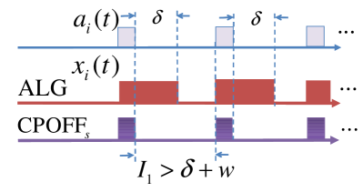
(a) $\delta+w\geq\beta_{s}/(d_{\min}P_{\min})$

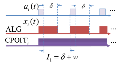
(b) $\delta+w<\beta_{s}/(d_{\min}P_{\min})$

Figure 10: Worst case examples.

For problem CP, consider the case that $d_{t}(0)=0$ and $a(t)\in[0,1],\ \forall t$. In this case, it is straightforward that $\textbf{CP}_{{\rm 1}}$ is equivalent to CP. Thus, the lower bound for $\textbf{CP}_{{\rm i}}$ is also a lower bound for CP. ∎

Theorem 4 follows from lemmas 6 and 7.

Appendix D Proof of Theorem 6

Instead of proving this theorem directly, we prove a stronger theorem that fully characterizes an offline optimal solution. Then Theorem 6 follows naturally. An very important structure of an offline optimal solution is “critical segments”, which are constructed according to $R_{i}(t)$.

Definition 1.

We divide all time intervals in $[1,T]$ into disjoint parts called critical segments:

$$[1,T_{1}^{c}],[T_{1}^{c}+1,T_{2}^{c}],[T_{2}^{c}+1,T_{3}^{c}],...,[T_{k}^{c}+1,T]$$

The critical segments are characterized by a set of critical points: $T_{1}^{c}<T_{2}^{c}<...<T_{k}^{c}$. We define each critical point $T_{j}^{c}$ along with an auxiliary point $\tilde{T_{j}^{c}}$, such that the pair $(T_{j}^{c},\tilde{T_{j}^{c}})$ satisfy the following conditions:

(Boundary): Either ($R_{i}(T_{j}^{c})=0$ and $R_{i}(\tilde{T_{j}^{c}})=-\beta_{g}$)
or ($R_{i}(T_{j}^{c})=-\beta_{g}$ and $R_{i}(\tilde{T_{j}^{c}})=0$).

(Interior): $-\beta<R_{i}(\tau)<0$ for all $T_{j}^{c}<\tau<\tilde{T_{j}^{c}}$.

In other words, each pair of $(T_{j}^{c},\tilde{T_{j}^{c}})$ corresponds to an interval where $R_{i}(t)$ goes from -$\beta_{g}$ to $0$ or $0$ to -$\beta_{g}$, without reaching the two extreme values inside the interval. For example, $(T_{1}^{c},\tilde{T_{1}^{c}})$ and $(T_{2}^{c},\tilde{T_{2}^{c}})$ in Fig. 11 are two such pairs, while the corresponding critical segments are $(T_{1}^{c},T_{2}^{c})$ and $(T_{2}^{c},T_{3}^{c})$. It is straightforward to see that all $(T_{j}^{c},\tilde{T_{j}^{c}})$ are uniquely defined, and hence critical segments are well-defined. See Fig. 11 for an example.

Figure 11: An example of critical segments.

Once the time horizon $[1,T]$ is divided into critical segments, we can now characterize the optimal solution.

Definition 2.

We classify the type of a critical segment by:

Type-start (also call type-0): $[1,T_{1}^{c}]$

Type-1: $[T_{j}^{c}+1,T_{j+1}^{c}]$, if $R_{i}(T_{j}^{c})=-\beta_{g}$ and $R_{i}(T_{j+1}^{c})=0$

Type-2: $[T_{j}^{c}+1,T_{j+1}^{c}]$, if $R_{i}(T_{j}^{c})=0$ and $R_{i}(T_{j+1}^{c})=-\beta_{g}$

Type-end (also call type-3): $[T_{k}^{c}+1,T]$

For completeness, we also let $T_{0}^{c}=0$ and $T_{k+1}^{c}=T$.

Then the following theorem characterizes an offline optimal solution.

Theorem 9.

An optimal solution for $\boldsymbol{EP_{i}}$ is given by

$$y_{{\rm OFA}}(t)\triangleq\begin{cases}0,&\mbox{if\ }t\in[T_{j}^{c}+1,T_{j+1}^{c}]\mbox{\ is type-start/-2/-end},\\ 1,&\mbox{if\ }t\in[T_{j}^{c}+1,T_{j+1}^{c}]\mbox{\ is type-1}.\end{cases}$$ (40)

Theorem 6 follows from Theorem 9 and Definition 2. Thus, it remains to prove Theorem 9.

D.1 Proof of Theorem 9

Before we prove the theorem, we introduce a lemma.

We define the cost with regard to a segment $j$ by:

$$\begin{array}[]{@{}r@{}l@{\ }l}&&{\rm C_{EP_{i}^{sg-j}}}(y)\\ &\triangleq&{\displaystyle\sum_{t=T_{j}^{c}+1}^{T_{j+1}^{c}}\psi\left(y(t),p(t),e_{i}(t)\right)}+{\displaystyle\sum_{t=T_{j}^{c}+1}^{T_{j+1}^{c}+1}\beta_{g}\cdot[y(t)-y(t-1)]^{+}}\end{array}$$

and define a subproblem for critical segment $j$ by:

$$\mathbf{EP_{i}}^{{\rm sg\mbox{-}j}}({\rm y}_{j}^{l},{\rm y}_{j}^{r}):\min\; {\rm C_{EP_{i}^{sg-j}}}(y)$$

s.t. $$y(T_{j}^{c})={\rm y}_{j}^{l},\;y(T_{j+1}^{c}+1)={\rm y}_{j}^{r},$$

var $$y(t)\in\{0,1\},t\in[T_{j}^{c}+1,T_{j+1}^{c}].$$

Note that due to the startup cost across segment boundaries, in general ${\rm C_{EP_{i}}}\neq\sum{\rm C_{EP_{i}^{sg-j}}}(y)$. In other words, we should not expect that putting together the solutions to each segment will lead to an overall offline optimal solution. However, the following lemma shows an important structure property that one optimal solution of $\mathbf{EP_{i}^{sg-j}}(y_{j}^{l},y_{j}^{r})$ is independent of boundary conditions $(y_{j}^{l},y_{j}^{r})$ although the optimal value depends on boundary conditions.

Lemma 8

$(y_{{\rm OFA}}(t))_{t=T_{j}^{c}+1}^{T_{j+1}^{c}}$ in (40) is an optimal solution for $\mathbf{EP_{i}^{sg-j}}(y_{j}^{l},y_{j}^{r})$, despite any boundary conditions $({\rm y}_{j}^{l},{\rm y}_{j}^{r})$.

We first use this lemma to prove Theorem 9 and then we prove this lemma. Suppose $(y^{\ast}(t))_{t=1}^{T}$ is an optimal solution for $\textbf{EP}_{{\rm i}}$. For completeness, we let $y^{\ast}(0)=0$ and $y^{\ast}(T+1)=0$. We define a sequence $(y_{0}(t))_{t=1}^{T},(y_{1}(t))_{t=1}^{T}$, $...,(y_{k+1}(t))_{t=1}^{T}$ as follows:

1. $y_{0}(t)=y^{\ast}(t)$ for all $t\in[1,T]$.

2. For all $t\in[1,T]$ and $j=1,...,k$

   $$y_{j}(t)=\begin{cases}y_{{\rm OFA}}(t),&\mbox{if\ }t\in[1,T_{j}^{c}]\\ y^{\ast}(t),&\mbox{otherwise\ }\end{cases}$$ (41)

3. $y_{k+1}(t)=y_{{\rm OFA}}(t)$ for all $t\in[1,T]$.

We next set the boundary conditions for each $\mathbf{EP_{i}^{sg-j}}$ by

$${\rm y}_{j}^{l}=y_{{\rm OFA}}(T_{j}^{c})\mbox{\ and\ }{\rm y}_{j}^{r}=y^{\ast}(T_{j+1}^{c}+1)$$ (42)

It follows that

$${\rm C_{EP_{i}}}(y_{j})-{\rm C_{EP_{i}}}(y_{j+1})={\rm C_{EP_{i}^{sg-j}}}(y^{\ast})-{\rm C_{EP_{i}^{sg-j}}}(y_{{\rm OFA}})$$ (43)

By Lemma 8, we obtain ${\rm C_{EP_{i}^{sg-j}}}(y^{\ast})\geq{\rm C_{EP_{i}^{sg-j}}}(y_{{\rm OFA}})$ for all $j$. Hence,

$${\rm C_{EP_{i}}}(y^{\ast})={\rm C_{EP_{i}}}(y_{0})\geq...\geq{\rm C_{EP_{i}}}(y_{k+1})={\rm C_{EP_{i}}}(y_{{\rm OFA}})$$ (44)

This completes the proof of Theorem 9.

Proof of Lemma 8: Consider given any boundary condition $({\rm y}_{j}^{l},{\rm y}_{j}^{r})$ for $\mathbf{EP_{i}^{sg-j}}$. Suppose $(\widehat{y}(t))_{t=T_{j}^{c}+1}^{T_{j+1}^{c}}$ is an optimal solution for $\mathbf{EP_{i}^{sg-j}}$ w.r.t. $({\rm y}_{j}^{l},{\rm y}_{j}^{r})$, and $\widehat{y}\neq y_{{\rm OFA}}$. We aim to show ${\rm C_{EP_{i}^{sg-j}}}(\widehat{y})\geq{\rm C_{EP_{i}^{sg-j}}}(y_{{\rm OFA}})$, by considering the types of critical segment.

(type-1): First, suppose that critical segment $[T_{j}^{c}+1,T_{j+1}^{c}]$ is type-1. Hence, $y_{{\rm OFA}}(t)=1$ for all $t\in[T_{j}^{c}+1,T_{j+1}^{c}]$. Hence,

$${\rm C_{EP_{i}^{sg-j}}}(y_{{\rm OFA}})=\beta_{g}\cdot(1-{\rm y}_{j}^{l})+\sum_{t=T_{j}^{c}+1}^{T_{j+1}^{c}}\psi\big{(}1,p(t),e_{i}(t)\big{)}$$ (45)

Case 1: Suppose $\widehat{y}(t)=0$ for all $t\in[T_{j}^{c}+1,T_{j+1}^{c}]$. Hence,

$${\rm C_{EP_{i}^{sg-j}}}(\widehat{y})=\beta_{g}\cdot{\rm y}_{j}^{r}+\sum_{t=T_{j}^{c}+1}^{T_{j+1}^{c}}\psi\big{(}0,p(t),e_{i}(t)\big{)}$$ (46)

We obtain:

$${\rm C_{EP_{i}^{sg-j}}}(\widehat{y})-{\rm C_{EP_{i}^{sg-j}}}(y_{{\rm OFA}})$$ (47)

$$= \beta_{g}\cdot{\rm y}_{j}^{r}+\sum_{t=T_{j}^{c}+1}^{T_{j+1}^{c}}r_{i}(t)-\beta_{g}(1-{\rm y}_{j}^{l})$$

$$\geq \beta_{g}\cdot{\rm y}_{j}^{r}+R_{i}(T_{j+1}^{c})-R_{i}(T_{j}^{c})-\beta_{g}(1-{\rm y}_{j}^{l})$$ (48)

$$= \beta_{g}\cdot{\rm y}_{j}^{r}+\beta_{g}-\beta_{g}+\beta_{g}{\rm y}_{j}^{l}\geq 0$$ (49)

where Eqn. (47) follows from the definition of $r_{i}(t)$ (see Eqn. (11)) and Eqn. (48) follows from Lemma 9. This completes the proof for Case 1.

(Case 2): Suppose $\widehat{y}(t)=1$ for some $t\in[T_{j}^{c}+1,T_{j+1}^{c}]$. This implies that ${\rm C_{EP_{i}^{sg-j}}}(\widehat{y})$ has to involve the startup cost $\beta_{g}$.

Next, we denote the minimal set of segments within $[T_{j}^{c}+1,T_{j+1}^{c}]$ by

$$[\tau_{1}^{b},\tau_{1}^{e}],[\tau_{2}^{b},\tau_{2}^{e}],[\tau_{3}^{b},\tau_{3}^{e}],...,[\tau_{p}^{b},\tau_{p}^{e}]$$

such that $\widehat{y}(t)\neq y_{{\rm OFA}}(t)$ for all $t\in[\tau_{l}^{b},\tau_{l}^{e}]$, $l\in\{1,...,p\}$, where $\tau_{l}^{e}<\tau_{l+1}^{b}$.

Since $\widehat{y}\neq y_{{\rm OFA}}$, then there exists at least one $t\in[T_{j}^{c}+1,T_{j+1}^{c}]$ such that $\widehat{y}(t)=0$. Hence, $\tau_{1}^{b}$ is well-defined.

Note that upon exiting each segment $[\tau_{l}^{b},\tau_{l}^{e}]$, $\widehat{y}$ switches from 0 to 1. Hence, it incurs the startup cost $\beta_{g}$. However, when $\tau_{p}^{e}=T_{j+1}^{c}$ and ${\rm y}_{j}^{r}=0$, the startup cost is not for critical segment $[T_{j}^{c}+1,T_{j+1}^{c}]$.

Therefore, we obtain:

$${\rm C_{EP_{i}^{sg-j}}}(\widehat{y})-{\rm C_{EP_{i}^{sg-j}}}(y_{{\rm OFA}})$$ (50)

$$= \sum_{t=\tau_{1}^{b}}^{\tau_{1}^{e}}r_{i}(t)+\beta_{g}\cdot\boldsymbol{1}[\tau_{1}^{b}\neq T_{j}^{c}+1]$$ (53)

$$+\sum_{l=2}^{p-1}\Big{(}\sum_{t=\tau_{l}^{b}}^{\tau_{l}^{e}}r_{i}(t)+\beta_{g}\Big{)}$$

$$+\sum_{t=\tau_{p}^{b}}^{\tau_{p}^{e}}r_{i}(t)+\beta_{g}{\rm y}_{j}^{r}\cdot\boldsymbol{1}[\tau_{p}^{e}=T_{j+1}^{c}]+\beta_{g}\cdot\boldsymbol{1}[\tau_{p}^{e}\neq T_{j+1}^{c}].$$

Now we prove the terms (53) (53) and (53) are all no less than $0.$

First, if $\tau_{1}^{b}=T_{j}^{c}+1,$ then

$$\sum_{t=\tau_{1}^{b}}^{\tau_{1}^{e}}r_{i}(t)+\beta_{g}\cdot\boldsymbol{1}[\tau_{1}^{b}\neq T_{j}^{c}+1] = \sum_{t=T_{j}^{c}+1}^{\tau_{1}^{e}}r_{i}(t)$$

$$\geq R_{i}(\tau_{1}^{e})-R_{i}(T_{j}^{c})$$

$$\geq R_{i}(\tau_{1}^{e})+\beta_{g}\geq 0.$$

else then

$$\sum_{t=\tau_{1}^{b}}^{\tau_{1}^{e}}r_{i}(t)+\beta_{g}\cdot\boldsymbol{1}[\tau_{1}^{b}\neq T_{j}^{c}+1] = \sum_{t=\tau_{1}^{b}}^{\tau_{1}^{e}}r_{i}(t)+\beta_{g}$$

$$\geq R_{i}(\tau_{1}^{e})-R_{i}(\tau_{1}^{b}-1)+\beta_{g}$$

$$\geq R_{i}(\tau_{1}^{e})+\beta_{g}\geq 0.$$

Thus, we proved (53)$\geq 0.$

Second,

$$\sum_{t=\tau_{l}^{b}}^{\tau_{l}^{e}}r_{i}(t)+\beta_{g} \geq R_{i}(\tau_{l}^{e})-R_{i}(\tau_{l}^{b}-1)+\beta_{g}$$

$$\geq R_{i}(\tau_{l}^{e})+\beta_{g}\geq 0.$$

Thus, we proved (53)$\geq 0.$

Last, if $\tau_{p}^{e}=T_{j+1}^{c},$ then

$$\sum_{t=\tau_{p}^{b}}^{\tau_{p}^{e}}r_{i}(t)+\beta_{g}{\rm y}_{i}^{r}\cdot\boldsymbol{1}[\tau_{p}^{e}=T_{j+1}^{c}]+\beta_{g}\cdot\boldsymbol{1}[\tau_{p}^{e}\neq T_{j+1}^{c}]$$

$$\geq \sum_{t=\tau_{p}^{b}}^{T_{j+1}^{c}}r_{i}(t)\geq R_{i}(T_{j+1}^{c})-R_{i}(\tau_{p}^{b}-1)$$

$$= -R_{i}(\tau_{p}^{b}-1)\geq 0.$$

else then

$$\sum_{t=\tau_{p}^{b}}^{\tau_{p}^{e}}r_{i}(t)+\beta_{g}{\rm y}_{i}^{r}\cdot\boldsymbol{1}[\tau_{p}^{e}=T_{j+1}^{c}]+\beta_{g}\cdot\boldsymbol{1}[\tau_{p}^{e}\neq T_{j+1}^{c}]$$

$$= \sum_{t=\tau_{p}^{b}}^{\tau_{p}^{e}}r_{i}(t)+\beta_{g}\geq R_{i}(\tau_{p}^{e})-R_{i}(\tau_{p}^{b}-1)+\beta_{g}$$

$$\geq 0.$$

Thus, we proved (53)$\geq 0.$

So we obtain

$${\rm C_{EP_{i}^{sg-j}}}(\widehat{y})-{\rm C_{EP_{i}^{sg-j}}}(y_{{\rm OFA}})\geq 0.$$

(type-2): Next, suppose that critical segment $[T_{j}^{c}+1,T_{j+1}^{c}]$ is type-2. Hence, $y_{{\rm OFA}}(t)=0$ for all $t\in[T_{j}^{c}+1,T_{j+1}^{c}]$. Note that the above argument applies similarly to type-2 setting, when we consider (Case 1): $\widehat{y}(t)=1$ for all $t\in[T_{j}^{c}+1,T_{j+1}^{c}]$ and (Case 2): $\widehat{y}(t)=0$ for some $t\in[T_{j}^{c}+1,T_{j+1}^{c}]$.

(type-start and type-end): We note that the argument of type-2 applies similarly to type-start and type-end settings.

Therefore, we complete the proof by showing ${\rm C_{EP_{i}^{sg-j}}}(\widehat{y})\geq{\rm C_{EP_{i}^{sg-j}}}(y_{{\rm OFA}})$ for all $j\in[0,k]$.

Lemma 9

Suppose $\tau_{1},\tau_{2}\in[T_{j}^{c}+1,T_{j+1}^{c}]$ and $\tau_{1}<\tau_{2}$. Then,

$$R_{i}(\tau_{2})-R_{i}(\tau_{1})\begin{cases}\leq\sum_{t=\tau_{1}+1}^{\tau_{2}}r_{i}(t),&\mbox{if\ }[T_{j}^{c}+1,T_{j+1}^{c}]\mbox{\ is type-1}\\ \geq\sum_{t=\tau_{1}+1}^{\tau_{2}}r_{i}(t),&\mbox{if\ }[T_{j}^{c}+1,T_{j+1}^{c}]\mbox{\ is type-2}\end{cases}$$ (54)

Proof.

We recall that

$$R_{i}(t)\triangleq\min\Big{\{}0,\max\{-\beta_{g},R_{i}(t-1)+r_{i}(t)\}\Big{\}}$$ (55)

First, we consider $[T_{j}^{c}+1,T_{j+1}^{c}]$ as type-1. This implies that only $R_{i}(T_{j}^{c})=-\beta_{g}$, whereas $R_{i}(t)>-\beta_{g}$ for $t\in[T_{j}^{c}+1,T_{j+1}^{c}]$. Hence,

$$R_{i}(t)=\min\{0,R_{i}(t-1)+r_{i}(t)\}\leq R_{i}(t-1)+r_{i}(t)$$ (56)

Iteratively, we obtain

$$R_{i}(\tau_{2})\leq R_{i}(\tau_{1})+\sum_{t=\tau_{1}+1}^{\tau_{2}}r_{i}(t)$$ (57)

When $[T_{j}^{c}+1,T_{j+1}^{c}]$ is type-2, we proceed with a similar proof, except

$$R_{i}(t)=\max\{-\beta_{g},R_{i}(t-1)+r_{i}(t)\}\geq R_{i}(t-1)+r_{i}(t)$$ (58)

Therefore,

$$R_{i}(\tau_{2})\geq R_{i}(\tau_{1})+\sum_{t=\tau_{1}+1}^{\tau_{2}}r_{i}(t).$$ (59)

∎

Appendix E Proof of Theorem 7

First, we denote the set of indexes of critical segments for type-$h$ by ${\cal T}_{h}\subseteq\{0,..,k\}$. Note that we also refer to type-start and type-end by type-0 and type-3 respectively.

Define the sub-cost for type-$h$ by

$${\rm C_{EP_{i}}^{{\rm ty\mbox{-}}h}}(y) \triangleq \sum_{j\in{\cal T}_{h}}\sum_{t=T_{j}^{c}+1}^{T_{j+1}^{c}}\psi\left(y(t),p(t),e_{i}(t)\right)$$

$$+\beta_{g}\cdot[y(t)-y(t-1)]^{+}.$$

Hence, ${\rm{\rm C_{EP_{i}}}}(y)=\sum_{h=0}^{3}{\rm C_{EP_{i}}^{{\rm ty\mbox{-}}h}}(y)$. We prove by comparing the sub-cost for each type-$h$. We denote the outcome of $\mathbf{CHASE_{s}^{(w)}}$ by $\big{(}y_{{\rm CHASE(w)}}(t)\big{)}_{t=1}^{T}.$

(type-0): Note that both $y_{{\rm OFA}}(t)=y_{{\rm CHASE(w)}}(t)=0$ for all $t\in[1,T_{1}^{c}]$. Hence,

$${\rm C_{EP_{i}}^{{\rm ty\mbox{-}}0}}(y_{{\rm OFA}})={\rm C_{EP_{i}}^{{\rm ty\mbox{-}}0}}(y_{{\rm CHASE(w)}}).$$

(type-1): Based on the definition of critical segment (Definition 1), we recall that there is an auxiliary point $\tilde{T_{j}^{c}}$, such that either ($R_{i}(T_{j}^{c})=0$ and $R_{i}(\tilde{T_{j}^{c}})=-\beta_{g}$) or ($R_{i}(T_{j}^{c})=-\beta_{g}$ and $R_{i}(\tilde{T_{j}^{c}})=0$). We focus on the segment $T_{j}^{c}+1+w<\tilde{T}_{j}^{c}$. We observe

$$y_{{\rm CHASE(w)}}(t)=\begin{cases}0,&\mbox{for all\ }t\in[T_{j}^{c}+1,\tilde{T}_{j}^{c}-w),\\ 1,&\mbox{for all\ }t\in[\tilde{T}_{j}^{c}-w,T_{j+1}^{c}].\end{cases}$$

We consider a particular type-1 critical segment, i.e., $k$-th type-1 critical segment: $[T_{j}^{c}+1,T_{j+1}^{c}]$. Note that by the definition of type-1, $y_{{\rm OFA}}(T_{j}^{c})=y_{{\rm CHASE(w)}}(T_{j}^{c})=0$. $y_{{\rm OFA}}(t)$ switches from $0$ to $1$ at time $T_{j}^{c}+1$, while $y_{{\rm CHASE(w)}}$ switches at time $\tilde{T}_{j}^{c}-w$, both incurring startup cost $\beta_{g}$. The cost difference between $y_{{\rm CHASE(w)}}$ and $y_{{\rm OFA}}$ within $[T_{j}^{c}+1,T_{j+1}^{c}]$ is

$$\sum_{t=T_{j}^{c}+1}^{\tilde{T}_{j}^{c}-w-1}\Big{(}\psi\left(0,p(t),e_{i}(t)\right)-\psi\Big{(}1,\sigma(t),e_{i}(t)\Big{)}\Big{)}+\beta_{g}-\beta_{g}$$

$$= \sum_{t=T_{j}^{c}+1}^{\tilde{T}_{j}^{c}-w-1}r_{i}(t)=R_{i}(\tilde{T}_{j}^{c}-w-1)-R_{i}(T_{j}^{c})=q_{k}^{1}+\beta_{g},$$

where $q_{k}^{1}\triangleq R_{i}(\tilde{T}_{j}^{c}-w-1)$.

Recall the number of type-$h$ critical segments $m_{h}\triangleq|{\cal T}_{h}|$.

$${\rm C_{EP_{i}}^{{\rm ty\mbox{-}}1}}(y_{{\rm CHASE(w)}})\leq{\rm C_{EP_{i}}^{{\rm ty\mbox{-}}1}}(y_{{\rm OFA}})+m_{1}\cdot\beta_{g}+\sum_{k=1}^{m_{1}}q_{k}^{1}.$$

(type-2) and (type-3): We derive similarly for $h=2$ or $3$ as

$${\rm C_{EP_{i}}^{{\rm ty\mbox{-}}h}}(y_{{\rm CHASE(w)}}) \leq {\rm C_{EP_{i}}^{{\rm ty\mbox{-}}h}}(y_{{\rm OFA}})-\sum_{k=1}^{m_{h}}q_{k}^{h}$$

$$\leq {\rm C_{EP_{i}}^{{\rm ty\mbox{-}}h}}(y_{{\rm OFA}})+\beta_{g}m_{h}.$$

The last inequality comes from that $q_{k}^{h}\geq-\beta_{g}$ for all $h,k$.

Furthermore, we note $m_{1}=m_{2}+m_{3}$. Overall, we obtain

$$\begin{array}[]{@{}r@{}l@{\ }l}&&{\displaystyle\frac{{\rm C_{EP_{i}}}(y_{{\rm CHASE(w)}})}{{\rm C_{EP_{i}}}(y_{{\rm OFA}})}}={\displaystyle\frac{\sum_{h=0}^{3}{\rm C_{EP_{i}}^{{\rm ty\mbox{-}}h}}(y_{{\rm CHASE(w)}})}{\sum_{h=0}^{3}{\rm C_{EP_{i}}^{{\rm ty\mbox{-}}h}}(y_{{\rm OFA}})}}\\ &\leq&{\displaystyle\frac{m_{1}\beta_{g}+\sum_{k=1}^{m_{1}}q_{k}^{1}+(m_{2}+m_{3})\beta_{g}+\sum_{h=0}^{3}{\rm C_{EP_{i}}^{{\rm ty\mbox{-}}h}}(y_{{\rm OFA}})}{\sum_{h=0}^{3}{\rm C_{EP_{i}}^{{\rm ty\mbox{-}}h}}(y_{{\rm OFA}})}}\\ &=&{\displaystyle 1+\frac{2m_{1}\beta_{g}+\sum_{k=1}^{m_{1}}q_{k}^{1}}{\sum_{h=0}^{3}{\rm C_{EP_{i}}^{{\rm ty\mbox{-}}h}}(y_{{\rm OFA}})}}\\ &\leq&1+\begin{cases}0&\mbox{if\ }m_{1}=0,\\ {\displaystyle\frac{2m_{1}\beta_{g}+\sum_{k=1}^{m_{1}}q_{k}^{1}}{{\rm C_{EP_{i}}^{{\rm ty\mbox{-}}1}}(y_{{\rm OFA}})}}&\mbox{otherwise}.\end{cases}\end{array}$$

By Lemma 10 and simplifications, we obtain

$${\displaystyle\frac{{\rm C_{EP_{i}}}(y_{{\rm CHASE(w)}})}{{\rm C_{EP_{i}}}(y_{{\rm OFA}})}}$$ (60)

$$\leq 1+\frac{2\beta_{g}\big{(}LP_{\max}-Lc_{o}-c_{m}\big{)}}{\beta_{g}LP_{\max}+w\cdot c_{m}P_{\max}\big{(}L-\frac{c_{m}}{P_{\max}-c_{o}}\big{)}\big{)}}$$

$$\leq 1+\frac{2\big{(}P_{\max}-c_{o}\big{)}}{P_{\max}(1+wc_{m}/\beta_{g})}.$$

Lemma 10

$${\rm C_{EP_{i}}^{{\rm ty\mbox{-}}1}}(y_{{\rm OFA}}) \geq m_{1}\beta_{g}+\sum_{k=1}^{m_{1}}\Big{(}\frac{(q_{k}^{1}+\beta_{g})(Lc_{o}+c_{m})}{LP_{\max}-Lc_{o}-c_{m}}$$

$$\quad+w\cdot c_{m}+\frac{c_{o}(-q_{k}^{1}+w\cdot c_{m})}{P_{\max}-c_{o}}\Big{)}$$

$$\geq \frac{m_{1}P_{\max}(\beta_{g}+wc_{m})}{P_{\max}-c_{o}}.$$

Proof.

Consider a particular type-1 segment $[T_{j}^{c}+1,T_{j+1}^{c}]$. Denote the costs of $\mathrm{y_{OFA}}$ during $[T_{j}^{c}+1,\tilde{T}_{j}^{c}-w-1]$ and $[\tilde{T}_{j}^{c}-w,T_{j+1}^{c}]$ by $\mathrm{Cost^{{\rm up}}}$ and $\mathrm{Cost^{{\rm pt}}}$ respectively.

Step 1: We bound $\mathrm{Cost^{{\rm up}}}$ as follows:

$$\mathrm{Cost^{{\rm up}}}$$ (61)

$$= \beta_{g}+\sum_{t=T_{j}^{c}+1}^{\tilde{T}_{j}^{c}-w-1}\psi\left(1,p(t),e_{i}(t)\right)$$

$$= \beta_{g}+(\tilde{T}_{j}^{c}-w-1-T_{j}^{c})c_{m}+\sum_{t=T_{j}^{c}+1}^{\tilde{T}_{j}^{c}-w-1}\big{(}\psi\left(1,p(t),e_{i}(t)\right)-c_{m}\big{)}.$$

On the other hand, we obtain

$$\sum_{t=T_{j}^{c}+1}^{\tilde{T}_{j}^{c}-w-1}\big{(}\psi\left(1,p(t),e_{i}(t)\right)-c_{m}\big{)}$$

$$= \frac{\sum_{t=T_{j}^{c}+1}^{\tilde{T}_{j}^{c}-w-1}\big{(}\psi\left(1,p(t),e_{i}(t)\right)-c_{m}\big{)}}{\sum_{t=T_{j}^{c}+1}^{\tilde{T}_{j}^{c}-w-1}\big{(}\psi\left(0,p(t),e_{i}(t)\right)-\psi\left(1,p(t),e_{i}(t)\right)+c_{m}\big{)}}$$

$$\times\sum_{t=T_{j}^{c}+1}^{\tilde{T}_{j}^{c}-w-1}\big{(}\psi\left(0,p(t),e_{i}(t)\right)-\psi\left(1,p(t),e_{i}(t)\right)+c_{m}\big{)}$$

$$\geq \min_{\tau\in[T_{j}^{c}+1,\tilde{T}_{j}^{c}-w-1]}\frac{\psi\left(1,p(\tau),e_{i}(\tau)\right)-c_{m}}{\psi\left(0,p(\tau),e_{i}(\tau)\right)-\psi\left(1,p(\tau),e_{i}(\tau)\right)+c_{m}}$$

$$\times\sum_{t=T_{j}^{c}+1}^{\tilde{T}_{j}^{c}-w-1}\big{(}\psi\left(0,p(t),e_{i}(t)\right)-\psi\left(1,p(t),e_{i}(t)\right)+c_{m}\big{)}$$

$$\geq \frac{c_{o}}{P_{\max}-c_{o}}$$

$$\times\sum_{t=T_{j}^{c}+1}^{\tilde{T}_{j}^{c}-w-1}\big{(}\psi\left(0,p(t),e_{i}(t)\right)-\psi\left(1,p(t),e_{i}(t)\right)+c_{m}\big{)}.$$

The last inequality follows from Lemma 11.

Next, we bound the second term by

$$\sum_{t=T_{j}^{c}+1}^{\tilde{T}_{j}^{c}-w-1}\big{(}\psi\left(0,p(t),e_{i}(t)\right)-\psi\left(1,p(t),e_{i}(t)\right)+c_{m}\big{)}$$

$$\geq \sum_{t=T_{j}^{c}+1}^{\tilde{T}_{j}^{c}-w-1}\big{(}r_{i}(t)+c_{m}\big{)}$$

$$\geq R_{i}\big{(}\tilde{T}_{j}^{c}-w-1\big{)}-R_{i}\big{(}T_{j}^{c}\big{)}+(\tilde{T}_{j}^{c}-w-1-T_{j}^{c})c_{m}$$

$$= q_{k}^{1}+\beta_{g}+(\tilde{T}_{j}^{c}-w-1-T_{j}^{c})c_{m}.$$

Together, we obtain

$$\mathrm{Cost^{{\rm up}}}$$ (63)

$$\geq \beta_{g}+(\tilde{T}_{j}^{c}-w-1-T_{j}^{c})c_{m}+$$

$$\frac{c_{o}}{P_{\max}-c_{o}}\Big{(}q_{k}^{1}+\beta_{g}+(\tilde{T}_{j}^{c}-w-1-T_{j}^{c})c_{m}\Big{)}$$

$$= \beta_{g}+\frac{(q_{k}^{1}+\beta_{g})c_{o}+(\tilde{T}_{j}^{c}-w-1-T_{j}^{c})P_{\max}c_{m}}{P_{\max}-c_{o}}.$$

Furthermore, we note that $\big{(}\tilde{T}_{j}^{c}-w-1-T_{j}^{c}\big{)}$ is lower bounded by the steepest descend when $p(t)=P_{\max}$ and $e_{i}(t)=L$,

$$\tilde{T}_{j}^{c}-w-1-T_{j}^{c}\geq\frac{q_{k}^{1}+\beta_{g}}{L\big{(}P_{\max}-c_{o}\big{)}-c_{m}}$$ (64)

By Eqns. (63)-(64), we obtain

$$\mathrm{Cost^{{\rm up}}}$$ (65)

$$\geq \beta_{g}+\frac{(q_{k}^{1}+\beta_{g})c_{o}+(\tilde{T}_{j}^{c}-w-1-T_{j}^{c})P_{\max}c_{m}}{P_{\max}-c_{o}}$$

$$\geq \beta_{g}+\frac{(q_{k}^{1}+\beta_{g})(Lc_{o}+c_{m})}{L\big{(}P_{\max}-c_{o}\big{)}-c_{m}}.$$

Step 2: We bound $\mathrm{Cost^{{\rm pt}}}$ as follows.

$$\mathrm{Cost^{{\rm pt}}}=\sum_{t=\tilde{T}_{j}^{c}-w}^{T_{j+1}^{c}}\psi\left(1,p(t),e_{i}(t)\right)$$

$$= (T_{j+1}^{c}-\tilde{T}_{j}^{c}+w+1)c_{m}+\sum_{t=\tilde{T}_{j}^{c}-w}^{T_{j+1}^{c}}\big{(}\psi\left(1,p(t),e_{i}(t)\right)-c_{m}\big{)}$$

$$\geq w\cdot c_{m}+$$

$$\frac{c_{o}}{P_{\max}-c_{o}}\sum_{t=\tilde{T}_{j}^{c}-w}^{T_{j+1}^{c}}\big{(}\psi\left(0,p(t),e_{i}(t)\right)-\psi\left(1,p(t),e_{i}(t)\right)+c_{m}\big{)}.$$

On the other hand, we obtain

$$\sum_{t=\tilde{T}_{j}^{c}-w}^{T_{j+1}^{c}}\big{(}\psi\left(0,p(t),e_{i}(t)\right)-\psi\left(1,p(t),e_{i}(t)\right)+c_{m}$$

$$= \sum_{t=\tilde{T}_{j}^{c}-w}^{T_{j+1}^{c}}r_{i}(t)+(T_{j+1}^{c}-\tilde{T}_{j}^{c}+w+1)c_{m}$$

$$\geq R_{i}(T_{j+1}^{c})-R_{i}(\tilde{T}_{j}^{c}-w-1)+w\cdot c_{m}=w\cdot c_{m}-q_{k}^{1}.$$

Therefore,

$$\mathrm{Cost^{{\rm pt}}} \geq w\cdot c_{m}+\frac{c_{o}(w\cdot c_{m}-q_{k}^{1})}{P_{\max}-c_{o}}.$$ (66)

Since there are $m_{1}$ type-1 critical segments, according to Eqns. (65)-(66), we obtain

$${\rm Cost}^{{\rm ty\mbox{-}}1}(y_{{\rm OFA}})$$

$$\geq m_{1}\beta_{g}+\sum_{k=1}^{m_{1}}\Big{(}\frac{(q_{k}^{1}+\beta_{g})(Lc_{o}+c_{m})}{L\big{(}P_{\max}-c_{o}\big{)}-c_{m}}$$

$$\qquad+w\cdot c_{m}+\frac{c_{o}(-q_{k}^{1}+w\cdot c_{m})}{P_{\max}-c_{o}}\Big{)}$$

$$\geq m_{1}\beta_{g}+\sum_{k=1}^{m_{1}}\Big{(}\frac{(q_{k}^{1}+\beta_{g})c_{o}}{\big{(}P_{\max}-c_{o}\big{)}}$$

$$\qquad+w\cdot c_{m}+\frac{c_{o}(-q_{k}^{1}+w\cdot c_{m})}{P_{\max}-c_{o}}\Big{)}$$

$$= m_{1}\beta_{g}+\frac{m_{1}(\beta_{g}c_{o}+P_{\max}wc_{m})}{P_{\max}-c_{o}}$$

$$= \frac{m_{1}P_{\max}(\beta_{g}+wc_{m})}{P_{\max}-c_{o}}.$$

∎

Lemma 11

$$\frac{\psi\left(1,p(\tau),e_{i}(\tau)\right)-c_{m}}{\psi\left(0,p(\tau),e_{i}(\tau)\right)-\psi\left(1,p(\tau),e_{i}(\tau)\right)+c_{m}}\geq\frac{c_{o}}{P_{\max}-c_{o}}.$$

Proof.

We expand $\psi\left(y(\tau),p(\tau),e_{i}(\tau)\right)$ for each case:

Case 1: $c_{o}\geq p(\tau)$. By Eqn. (2.2) and $e_{i}(\tau)\leq L,\forall i,\tau$,

$$\psi\left(1,p(\tau),e_{i}(\tau)\right) = p(\tau)e_{i}(\tau)+c_{m},$$

$$\psi\left(0,p(\tau),e_{i}(\tau)\right) = p(\tau)e_{i}(\tau).$$

Therefore,

$$\frac{\psi\left(1,p(t),e_{i}(t)\right)-c_{m}}{\psi\left(0,p(t),e_{i}(t)\right)-\psi\left(1,p(t),e_{i}(t)\right)+c_{m}}=\infty.$$

Case 2: $c_{o}<p(\tau)$. By Eqn. (2.2) and $e_{i}(\tau)\leq L,\forall i,\tau$,

Thus,

$$\psi\left(1,p(\tau),e_{i}(\tau)\right) = c_{o}e_{i}(\tau)+c_{m},$$

$$\psi\left(0,p(\tau),e_{i}(\tau)\right) = p(\tau)e_{i}(\tau).$$

Therefore,

$$\frac{\psi\left(1,p(\tau),e_{i}(\tau)\right)-c_{m}}{\psi\left(0,p(\tau),e_{i}(\tau)\right)-\psi\left(1,p(\tau),e_{i}(\tau)\right)+c_{m}}$$

$$\geq \frac{c_{o}e_{i}(\tau)}{p(\tau)e_{i}(\tau)-c_{o}e_{i}(\tau)}$$

$$\geq \frac{c_{o}}{P_{\max}-c_{o}}.$$

Combining both cases, we complete the proof of this lemma.∎

Appendix F Proof of Theorem 2

First, we prove that the factor loss in optimality is at most $LP_{\max}/\left(Lc_{o}+c_{m}\right)$.

Then, we prove that the factor loss is tight.

Let $(\boldsymbol{\bar{x}},\boldsymbol{\bar{y}})$ be the solution obtained by solving CP and EP separately in sequence and $\left(\boldsymbol{x}^{*},\boldsymbol{y}^{*}\right)$ be the solution obtained by solving the joint-optimization DCM. Denote ${\rm C_{DCM}}(\boldsymbol{x},\boldsymbol{y})$ to be cost of DCM of solution $(\boldsymbol{x},\boldsymbol{y})$ and ${\rm C_{CP}}(\boldsymbol{x})$ to be cost of CP of solution $\boldsymbol{x}$.

It is straightforward that

$${\rm C_{DCM}}(\boldsymbol{\bar{x}},\boldsymbol{\bar{y}})\leq{\rm C_{DCM}}(\boldsymbol{\bar{x}},\boldsymbol{0}).$$ (67)

Because ${\rm C_{DCM}}(\boldsymbol{x},0)={\rm C_{CP}}(\boldsymbol{x}),$ we have

$${\rm C_{DCM}}(\boldsymbol{\bar{x}},\boldsymbol{0})={\rm C_{CP}}(\boldsymbol{\bar{x}})\leq{\rm C_{CP}}(\boldsymbol{x}^{*})={\rm C_{DCM}}(\boldsymbol{x}^{*},\boldsymbol{0}).$$ (68)

By Eqns. (67) and (68), we obtain

$$\frac{{\rm C_{DCM}}(\boldsymbol{\bar{x}},\boldsymbol{\bar{y}})}{{\rm C_{DCM}}(\boldsymbol{x}^{*},\boldsymbol{y}^{*})}\leq\frac{{\rm C_{DCM}}(\boldsymbol{x}^{*},\boldsymbol{0})}{{\rm C_{DCM}}(\boldsymbol{x}^{*},\boldsymbol{y}^{*})}.$$ (69)

Then, according to the following lemma, we get

$$\rho=\frac{{\rm C_{DCM}}(\boldsymbol{\bar{x}},\boldsymbol{\bar{y}})}{{\rm C_{DCM}}(\boldsymbol{x}^{*},\boldsymbol{y}^{*})}\leq\frac{LP_{\max}}{Lc_{o}+c_{m}}.$$

Lemma 12

${\rm C_{DCM}}(\boldsymbol{x}^{*},\boldsymbol{0})/{\rm C_{DCM}}(\boldsymbol{x}^{*},\boldsymbol{y}^{*})\leq LP_{\max}/\left(Lc_{o}+c_{m}\right).$

Proof.

By plugging solutions $(\boldsymbol{x}^{*},\boldsymbol{0})$ and $(\boldsymbol{x}^{*},\boldsymbol{y}^{*})$ into DCM separately, we have

$${\rm C_{DCM}}(\boldsymbol{x}^{*},\boldsymbol{0}) = \sum_{t=1}^{T}\left\{p(t)d_{t}\left(x^{*}(t)\right)\right.$$ (70)

$$\left.+\beta_{s}[x^{*}(t)-x^{*}(t-1)]^{+}\right\}$$

and

$${\rm C_{DCM}}(\boldsymbol{x}^{*},\boldsymbol{y}^{*}) = \sum_{t=1}^{T}\left\{\psi\left(y^{*}(t),p(t),d_{t}\left(x^{*}(t)\right)\right)\right.$$ (71)

$$+\beta_{s}[x^{*}(t)-x^{*}(t-1)]^{+}$$

$$\left.+\beta_{g}[y^{*}(t)-y^{*}(t-1)]^{+}\right\}$$

$$\geq \sum_{t=1}^{T}\left\{\psi\left(y^{*}(t),p(t),d_{t}\left(x^{*}(t)\right)\right)\right.$$

$$\left.+\beta_{s}[x^{*}(t)-x^{*}(t-1)]^{+}\right\}.$$

By Eqns. (70), (71) and (2.2), we obtain

$$\frac{{\rm C_{DCM}}(\boldsymbol{x}^{*},\boldsymbol{0})}{{\rm C_{DCM}}(\boldsymbol{x}^{*},\boldsymbol{y}^{*})}$$

$$\leq \frac{\sum_{t=1}^{T}p(t)d_{t}\left(x^{*}(t)\right)}{\sum_{t=1}^{T}\psi\left(y^{*}(t),p(t),d_{t}\left(x^{*}(t)\right)\right)}$$

$$\leq \max_{t\in\{1,..,T\}}\frac{p(t)d_{t}\left(x^{*}(t)\right)}{\psi\left(y^{*}(t),p(t),d_{t}\left(x^{*}(t)\right)\right)}$$

$$\leq \begin{cases}1,&\mbox{if }p(t)\leq c_{o},\\ \frac{P_{\max}d_{t}\left(x^{*}(t)\right)}{c_{o}d_{t}\left(x^{*}(t)\right)+c_{m}\left\lceil d_{t}\left(x^{*}(t)\right)/L\right\rceil},&\mbox{otherwise}\end{cases}$$

$$\leq \frac{P_{\max}d_{t}\left(x^{*}(t)\right)}{c_{o}d_{t}\left(x^{*}(t)\right)+c_{m}d_{t}\left(x^{*}(t)\right)/L}$$

$$= \frac{P_{\max}}{c_{o}+c_{m}/L}.$$

∎

Next, we prove that the factor loss is tight.

Lemma 13

There exist an input such that
${\rm C_{DCM}}(\boldsymbol{\bar{x}},\boldsymbol{\bar{y}})/{\rm C_{DCM}}(\boldsymbol{x}^{*},\boldsymbol{y}^{*})=LP_{\max}/\left(Lc_{o}+c_{m}\right).$

Proof.

Consider the following input:

$$d_{t}(x(t))=e_{m}x(t),\ p(t)=P_{\max},\ \forall t,$$

and

$$a(t)=\begin{cases}\frac{L}{e_{m}},&\mbox{if }t=1+k(1+\frac{\beta_{s}}{e_{m}P_{\max}}),\ k\in\mathbb{N}^{0},\\ 0,&\mbox{otherwise,}\end{cases}$$

where $e_{m}>0$ is a constant such that $L/e_{m}$ is an integer.

Then for the above input, according to algorithm 3, it is easy to see that

$$\bar{x}(t)=\begin{cases}\frac{L}{e_{m}},&\mbox{if }t=1+k(1+\frac{\beta_{s}}{e_{m}P_{\max}}),\ k\in\mathbb{N}^{0},\\ 0,&\mbox{otherwise.}\end{cases}$$

Besides, according to algorithm 3, the following $\boldsymbol{x}^{*}$ must be an optimal solution whatever $y^{*}$ is.

$$x^{*}(t)=\frac{L}{e_{m}},\ \forall t.$$

Without loss of generality, consider the following parameter setting:

$$L(P_{\max}-c_{o})-c_{m}<\beta_{g},$$

$$L(P_{\max}-c_{o})-c_{m}-\frac{\beta_{s}}{e_{m}P_{\max}}c_{m}<0,$$

and

$$L(P_{\max}-c_{o})-c_{m}-\frac{\beta_{s}}{e_{m}P_{\max}}c_{m}+\frac{\beta_{s}L}{e_{m}P_{\max}}(P_{\max}-c_{o})>0.$$

Since $\bar{\boldsymbol{x}}$ and $\boldsymbol{x}^{*}$ have been determined by us, we can apply Theorem 9 to obtain the corresponding $\boldsymbol{\bar{y}}$ and $\boldsymbol{y}^{*}$. According to Eqn. (11) and the above parameter setting, given $\bar{\boldsymbol{x}}$ and $\boldsymbol{a}$, the corresponding $R_{i}(t)$ never reaches 0. However, given $\boldsymbol{x}^{*}$ and $\boldsymbol{a}$, the corresponding $R_{i}(t)$ will soon reach 0 and never fall back to $-\beta_{g}$. So we have

$$\bar{y}(t)=0,\ \forall t$$

and

$$y^{*}(t)=1,\ \forall t.$$

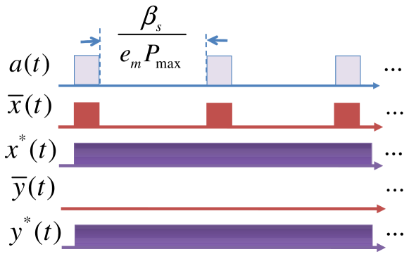
Figure 12: Example of $a(t)$, $\bar{x}(t)$, $x^{*}(t)$, $\bar{y}(t)$ and $y^{*}(t)$.

See Fig. 12 as an example. By plugging the above $(\boldsymbol{\bar{x}},\boldsymbol{\bar{y}})$ and $\left(\boldsymbol{x}^{*},\boldsymbol{y}^{*}\right)$ into DCM, we have

$$\frac{{\rm C_{DCM}}(\boldsymbol{\bar{x}},\boldsymbol{\bar{y}})}{{\rm C_{DCM}}(\boldsymbol{x}^{*},\boldsymbol{y}^{*})} = \frac{LP_{\max}+\beta_{s}L/e_{m}}{Lc_{o}+c_{m}+(Lc_{o}+c_{m})\beta_{s}/(e_{m}P_{\max})}$$

$$= \frac{LP_{\max}\left[1+\beta_{s}/(e_{m}P_{\max})\right]}{(Lc_{o}+c_{m})\left[1+\beta_{s}/(e_{m}P_{\max})\right]}$$

$$= \frac{LP_{\max}}{Lc_{o}+c_{m}}.$$

∎

Theorem 2 follows from Eqn. (69), lemmas 12 and 13.

Appendix G Proof of Theorem 8

Let $(\boldsymbol{\bar{x}},\boldsymbol{\bar{y}})$ be an offline optimal solution obtained by solving CP and EP separately in sequence and $\left(\boldsymbol{x}^{*},\boldsymbol{y}^{*}\right)$ be an offline optimal solution obtained by solving the joint-optimization DCM. Let $\boldsymbol{x^{on}}$ be the solution obtained by $\mathbf{GCSR^{(w)}}$ and $\boldsymbol{y^{off}}$ be an offline optimal solution of EP given input $\boldsymbol{x^{on}}$. Let $\left(\boldsymbol{x^{on}},\boldsymbol{y^{on}}\right)$ be the solution obtained by $\mathbf{DCMON^{(w)}}$. Denote ${\rm C_{DCM}}(\boldsymbol{x},\boldsymbol{y})$ to be cost of DCM of solution $(\boldsymbol{x},\boldsymbol{y})$ and ${\rm C_{CP}}(\boldsymbol{x})$ to be cost of CP of solution $\boldsymbol{x}$.

According to Theorem 7, equation (60) and the fact that the available look-ahead window size is only $\left[w-\Delta_{s}\right]^{+}$ for $\mathbf{DCMON^{(w)}}$ to solve EP (discussed in Sec. 5.3), we have

$$\frac{{\rm C_{DCM}}(\boldsymbol{x^{on}},\boldsymbol{y^{on}})}{{\rm C_{DCM}}(\boldsymbol{x^{on}},\boldsymbol{y^{off}})}$$ (72)

$$\leq 1+\frac{2\beta_{g}\left(LP{}_{\max}-Lc_{o}-c_{m}\right)}{\beta_{g}LP{}_{\max}+\left[w-\Delta_{s}\right]^{+}c_{m}P{}_{\max}\left(L-\frac{c_{m}}{P{}_{\max}-c_{o}}\right)}$$

$$\leq 1+\frac{2\left(LP{}_{\max}-Lc_{o}-c_{m}\right)}{LP{}_{\max}+\alpha_{g}P{}_{\max}\left(L-\frac{c_{m}}{P{}_{\max}-c_{o}}\right)}$$

$$\leq 1+2\frac{P_{\max}-c_{o}}{P_{\max}}\cdot\frac{1}{1+\alpha_{g}},$$

where $\triangle_{s}\triangleq\beta_{s}/(d_{\min}P_{\min})$ and $\alpha_{g}\triangleq\frac{c_{m}}{\beta_{g}}\left[w-\Delta_{s}\right]^{+}$ is a “normalized” look-ahead window size that takes values in $[0,+\infty)$.

According to Theorem 2, we have

$$\frac{{\rm C_{DCM}}(\boldsymbol{\bar{x}},\boldsymbol{\bar{y}})}{{\rm C_{DCM}}\left(\boldsymbol{x}^{*},\boldsymbol{y}^{*}\right)}\leq\frac{LP_{\max}}{Lc_{o}+c_{m}}.$$ (73)

Then if we can bound ${\rm C_{DCM}}(\boldsymbol{x^{on}},\boldsymbol{y^{off}})/{\rm C_{DCM}}(\boldsymbol{\bar{x}},\boldsymbol{\bar{y}})$, we obtain the competitive ratio upper bound of $\mathbf{DCMON^{(w)}}$. The following lemma gives us such a bound.

Lemma 14

${\rm C_{DCM}}(\boldsymbol{x^{on}},\boldsymbol{y^{off}})/{\rm C_{DCM}}(\boldsymbol{\bar{x}},\boldsymbol{\bar{y}})\leq 2-\alpha_{s}$, where $\alpha_{s}\triangleq\min\left(1,w/\triangle_{s}\right)$ and $\triangle_{s}\triangleq\beta_{s}/(d_{\min}P_{\min})$.

Proof.

It is straightforward that

$${\rm C_{DCM}}(\boldsymbol{x^{on}},\boldsymbol{y^{off}})\leq{\rm C_{DCM}}(\boldsymbol{x^{on}},\boldsymbol{\bar{y}}).$$ (74)

So we seeks to bound ${\rm C_{DCM}}(\boldsymbol{x^{on}},\boldsymbol{\bar{y}})/{\rm C_{DCM}}(\boldsymbol{\bar{x}},\boldsymbol{\bar{y}})$.

For solution $\boldsymbol{x^{on}}$ and $\boldsymbol{\bar{x}}$, denote

$$CW(\boldsymbol{x})=\beta_{s}\sum_{t=1}^{T}\left[x(t)-x(t-1)\right]^{+},$$ (75)

and

$$CI(\boldsymbol{x^{on}},\boldsymbol{\bar{x}})=\sum_{t=1}^{T}p(t)\left(d_{t}(x^{on}(t))-d_{t}(\bar{x}(t))\right).$$ (76)

According to Eqn. (36), we have

$$CW(\boldsymbol{x_{i}^{on}})=CW(\boldsymbol{\bar{x}}_{i}).$$ (77)

According to lemma 15 and the fact that $x_{i}^{on}(t),\bar{x}_{i}(t)\in\{0,1\},\ \forall t,i$, we have

$$CW(\boldsymbol{x^{on}}) = CW(\sum_{i=1}^{M}\boldsymbol{x_{i}^{on}})=\sum_{i=1}^{M}CW(\boldsymbol{x_{i}^{on}})$$ (78)

$$= \sum_{i=1}^{M}CW(\boldsymbol{\bar{x}}_{i})=CW(\sum_{i=1}^{M}\boldsymbol{\bar{x}}_{i})$$

$$= CW(\boldsymbol{\bar{x}}),$$

and

$$CI(\boldsymbol{x^{on}},\boldsymbol{\bar{x}}) = \sum_{t=1}^{T}p(t)\left(d_{t}(x^{on}(t))-d_{t}(\bar{x}(t))\right)$$ (79)

$$= \sum_{t=1}^{T}p(t)\left(\sum_{i=1}^{x^{on}(t)}d_{t}^{i}-\sum_{i=1}^{\bar{x}(t)}d_{t}^{i}\right)$$

$$= \sum_{i=1}^{M}\sum_{t=1}^{T}p(t)d_{t}^{i}(x_{i}^{on}(t)-\bar{x}_{i}(t))$$

$$\leq (1-\alpha_{s})\sum_{i=1}^{M}CW(\boldsymbol{\bar{x}_{i}})$$

$$= (1-\alpha_{s})CW(\boldsymbol{\bar{x}}),$$

where the last and second last inequalities come from Eqns. (78) and (39), respectively.

According to Eqn. (2.2), we have $\forall b\in[0,x^{on}(t)]$,

$$\psi\left(\bar{y}(t),p(t),d_{t}\left(x^{on}(t)\right)\right)-\psi\left(\bar{y}(t),p(t),d_{t}\left(b\right)\right)$$ (80)

$$\leq p(t)\left(d_{t}\left(x^{on}(t)\right)-d_{t}\left(b\right)\right).$$

By the definition of DCM, Eqns. (37), (75), (76) and (80),

$${\rm C_{DCM}}(\boldsymbol{x^{on}},\boldsymbol{\bar{y}})$$ (81)

$$= \sum_{t=1}^{T}\left\{\psi\left(\bar{y}(t),p(t),d_{t}\left(x^{on}(t)\right)\right)\right.$$

$$\left.+\beta_{s}[x^{on}(t)-x^{on}(t-1)]^{+}+\beta_{g}[\bar{y}(t)-\bar{y}(t-1)]^{+}\right\}$$

$$\leq \sum_{t=1}^{T}\left\{\psi\left(\bar{y}(t),p(t),d_{t}\left(\bar{x}(t)\right)\right)+p(t)\left(d_{t}\left(x^{on}(t)\right)-d_{t}\left(\bar{x}(t)\right)\right)\right.$$

$$\left.+\beta_{s}[x^{on}(t)-x^{on}(t-1)]^{+}+\beta_{g}[\bar{y}(t)-\bar{y}(t-1)]^{+}\right\}$$

$$= \sum_{t=1}^{T}\left\{\psi\left(\bar{y}(t),p(t),d_{t}\left(\bar{x}(t)\right)\right)+\beta_{g}[\bar{y}(t)-\bar{y}(t-1)]^{+}\right\}$$

$$+CW(\boldsymbol{x_{on}})+CI(\boldsymbol{x_{on}},\boldsymbol{\bar{x}}).$$

Then, by Eqns. (78), (79) and (81), we have

$$\frac{{\rm C_{DCM}}(\boldsymbol{x_{on}},\boldsymbol{\bar{y}})}{{\rm C_{DCM}}\left(\boldsymbol{\bar{x}},\boldsymbol{\bar{y}}\right)}$$ (82)

$$\leq \frac{\sum_{t=1}^{T}\psi\left(\bar{y}(t),p(t),d_{t}\left(\bar{x}(t)\right)\right)+CI(\boldsymbol{x_{on}},\boldsymbol{\bar{x}})+CW(\boldsymbol{x_{on}})}{\sum_{t=1}^{T}\psi\left(\bar{y}(t),p(t),d_{t}\left(\bar{x}(t)\right)\right)+CW(\boldsymbol{\bar{x}})}$$

$$\leq \frac{(1-\alpha_{s})CW(\boldsymbol{\bar{x}})+CW(\boldsymbol{x_{on}})}{CW(\boldsymbol{\bar{x}})}$$

$$= \frac{(1-\alpha_{s})CW(\boldsymbol{\bar{x}})+CW(\boldsymbol{\bar{x}})}{CW(\boldsymbol{\bar{x}})}$$

$$= 2-\alpha_{s}.$$

This lemma follows from Eqns. (74) and (82). ∎

Theorem 8 follows from Eqns. (72), (73) and lemma 14.

Lemma 15

$\boldsymbol{\bar{x}_{1}},\boldsymbol{\bar{x}_{2}},\ldots\boldsymbol{\bar{x}_{M}}$ and $\boldsymbol{x_{1}^{on}},\boldsymbol{x_{2}^{on}},\ldots\boldsymbol{x_{M}^{on}}$ are decreasing sequences, i.e., $\forall t,\ \bar{x}_{1}(t)\geq...\geq\bar{x}_{M}(t)\ \mbox{and}\ x_{1}^{on}(t)\geq...\geq x_{M}^{on}(t).$

Proof.

Recall that $\boldsymbol{\bar{x}_{i}}$ and $\boldsymbol{x_{i}^{on}}$ are offline and online solutions obtained by $\mathbf{CPOFF_{s}}$ and $\mathbf{GCSR_{s}^{(w)}}$ for problem $\textbf{CP}_{{\rm i}}$, respectively. According to the definition of $\textbf{CP}_{{\rm i}}$, $a_{1}(t)\geq a_{2}(t)\geq...\geq a_{M}(t)$ is a decreasing sequence and $d_{t}^{1}\leq d_{t}^{2}\leq...\leq d_{t}^{M}$ is an increasing sequence. Thus, for problem $\textbf{CP}_{{\rm i}}$, the larger the index $i$ is, the more sparse workload tends to be and the higher power consumption tends to be. Hence, for a larger index $i$, there are more “idling intervals”, meanwhile both $\mathbf{CPOFF_{s}}$ and $\mathbf{GCSR_{s}^{(w)}}$ tends to keep servers idling less during idling intervals (because idling cost is higher). So, $\boldsymbol{\bar{x}_{1}},\boldsymbol{\bar{x}_{2}},\ldots\boldsymbol{\bar{x}_{M}}$ and $\boldsymbol{x_{1}^{on}},\boldsymbol{x_{2}^{on}},\ldots\boldsymbol{x_{M}^{on}}$ are decreasing sequences, i.e., $\forall t,\ \bar{x}_{1}(t)\geq...\geq\bar{x}_{M}(t)\ \mbox{and}\ x_{1}^{on}(t)\\ \geq...\geq x_{M}^{on}(t).$∎

References

- [1] Akamai tech. http://www.akamai.com.
- [2] Nationalgrid. https://www.nationalgridus.com/.
- [3] Pacific gas and electric company. http://www.pge.com/nots/rates/tariffs/rateinfo.shtml.
- [4] Tecogen. http://www.tecogen.com.
- [5] The weather channal. http://www.weather.com/.
- [6] Apple’s onsite renewable energy, 2012. http://www.apple.com/environment/renewable-energy/.
- [7] Distributed generation, 2012. http://www.bloomenergy.com/fuel-cell/distributed-generation/.
- [8] C. Baldwin, K. Dale, and R. Dittrich. A study of the economic shutdown of generating units in daily dispatch. IEEE Trans. Power Apparatus and Systems, 1959.
- [9] L. Barroso and U. Holzle. The case for energy-proportional computing. IEEE Computer, 2007.
- [10] A. Beloglazov, R. Buyya, Y. Lee, and A. Zomaya. A taxonomy and survey of energy-efficient data centers and cloud computing systems. Advances in Computers, 2011.
- [11] A. Borbely and J. Kreider. Distributed generation: the power paradigm for the new millennium. CRC Press, 2001.
- [12] A. Borodin and R. El-Yaniv. Online computation and competitive analysis. Cambridge University Press, 1998.
- [13] J. Chase, D. Anderson, P. Thakar, A. Vahdat, and R. Doyle. Managing energy and server resources in hosting centers. In Proc. ACM SIGOPS, 2001.
- [14] A.J. Conejo, M.A. Plazas, R. Espinola, and A.B. Molina. Day-ahead electricity price forecasting using the wavelet transform and arima models. Power Systems, IEEE Transactions on, 2005.
- [15] E. Dijkstra. A note on two problems in connexion with graphs. Numerische mathematik, 1959.
- [16] R. Doyle, J. Chase, O. Asad, W. Jin, and A. Vahdat. Model-based resource provisioning in a web service utility. In Proc. USITS, 2003.
- [17] K. Fehrenbacher. ebay to build huge bloom energy fuel cell farm at data center. 2012. http://gigaom.com/cleantech/ebay-to-build-huge-bloom-energy-fuel-cell-farm-at-data-center/.
- [18] K. Fehrenbacher. Is it time for more off-grid options for data centers. 2012. http://gigaom.com/cleantech/is-it-time-for-more-off-grid-options-for-data-centers/.
- [19] Daniel Gmach, Jerry Rolia, Ludmila Cherkasova, and Alfons Kemper. Workload analysis and demand prediction of enterprise data center applications. In Workload Characterization, 2007. IISWC 2007. IEEE 10th International Symposium on, 2007.
- [20] S. Kazarlis, A. Bakirtzis, and V. Petridis. A genetic algorithm solution to the unit commitment problem. IEEE Trans. Power Systems, 1996.
- [21] J. Koomey. Growth in data center electricity use 2005 to 2010. Analytics Press, 2010.
- [22] M. Lin, Z. Liu, A. Wierman, and L. Andrew. Online algorithms for geographical load balancing. In Proc. IEEE IGCC, 2012.
- [23] M. Lin, A. Wierman, L. Andrew, and E. Thereska. Dynamic right-sizing for power-proportional data centers. In Proc. IEEE INFOCOM, 2011.
- [24] Z. Liu, Y. Chen, C. Bash, A. Wierman, D. Gmach, Z. Wang, M. Marwah, and C. Hyser. Renewable and cooling aware workload management for sustainable data centers. In Proc. ACM SIGMETRICS, 2012.
- [25] J. Lowesohn. Apple’s main data center to go fully renewable this year. 2012. http://news.cnet.com/8301-13579_3-57436553-37/apples-main-data-center-to-go-fully-renewable-this-year/.
- [26] L. Lu, J. Tu, C. Chau, M. Chen, and X. Lin. Online energy generation scheduling for microgrids with intermittent energy sources and co-generation. In Proc. ACM SIGMETRICS, 2013.
- [27] T. Lu and Chen M. Simple and effective dynamic provisioning for power-proportional data centers. In Proc. IEEE CISS, 2012.
- [28] V. Mathew, R. Sitaraman, and P. Shenoy. Energy-aware load balancing in content delivery networks. In Proc. IEEE INFOCOM, 2012.
- [29] J. Muckstadt and R. Wilson. An application of mixed-integer programming duality to scheduling thermal generating systems. IEEE Trans. Power Apparatus and Systems, 1968.
- [30] E. Nygren, R. Sitaraman, and J. Sun. The Akamai Network: A platform for high-performance Internet applications. 2010.
- [31] N. Padhy. Unit commitment-a bibliographical survey. IEEE Trans. Power Systems, 2004.
- [32] D. Palasamudram, R. Sitaraman, B. Urgaonkar, and R. Urgaonkar. Using batteries to reduce the power costs of internet-scale distributed networks. In Proc. ACM Symposium on Cloud Computing, 2012.
- [33] S. Pelley, D. Meisner, T. Wenisch, and J. VanGilder. Understanding and abstracting total data center power. In Workshop on Energy-Efficient Design, 2009.
- [34] E. Pinheiro, R. Bianchini, E. Carrera, and T. Heath. Load balancing and unbalancing for power and performance in cluster-based systems. In Workshop on compilers and operating systems for low power, 2001.
- [35] A. Qureshi, R. Weber, H. Balakrishnan, J. Guttag, and B. Maggs. Cutting the electric bill for internet-scale systems. In Proc. ACM SIGCOMM, 2009.
- [36] T. Shiina and J. Birge. Stochastic unit commitment problem. International Trans. Operational Research, 2004.
- [37] M. Stadler, H. Aki, R. Lai, C. Marnay, and A. Siddiqui. Distributed energy resources on-site optimization for commercial buildings with electric and thermal storage technologies. Lawrence Berkeley National Laboratory, 2008.
- [38] R. Stanojevic and R. Shorten. Distributed dynamic speed scaling. In Proc. IEEE INFOCOM, 2010.
- [39] H. Xu, C. Feng, and B. Li. Temperature aware workload management in geo-distributed datacenters. In Proc. ACM SIGMETRICS, extended abstract, 2013.