A second note on the discrete Gaussian Free Field
with disordered pinning on $\mathbb{Z}^{d}$, $d\geq 2$

Loren Coquille, Piotr MiΕ‚oΕ›
Abstract

We study the discrete massless Gaussian Free Field on $\mathbb{Z}^{d}$, $d\geq 2$, in the presence of a disordered square-well potential supported on a finite strip around zero. The disorder is introduced by reward/penalty interaction coefficients, which are given by i.i.d. random variables.

In the previous note [4], we proved under minimal assumptions on the law of the environment, that the quenched free energy associated to this model exists in $\mathbb{R}^{+}$, is deterministic, and strictly smaller than the annealed free energy whenever the latter is strictly positive.

Here we consider Bernoulli reward/penalty coefficientsΒ bβ‹…ex+h⋅𝑏subscript𝑒π‘₯β„Žb\cdot e_{x}+h with $e_{x}\sim\text{Bernoulli}_{1/2}(-1,+1)$ for all $x\in\mathbb{Z}^{d}$, and $b>0$, $h\in\mathbb{R}$. We prove that in the plane $(b,h)$, the quenched critical line (separating the phases of positive and zero free energy) lies strictly below the line $h=0$, showing in particular that there exists a non trivial region where the field is localized though repulsed on average by the environment.

Keywords : Random interfaces, random surfaces, pinning, disordered systems, Gaussian free field.
MSC2010 : 60K35, 82B44, 82B41.

1 The model

We study the discrete Gaussian Free Field with a disordered square-well potential. For $\Lambda$ a finite subset of $\mathbb{Z}^{d}$, denoted by $\Lambda\Subset\mathbb{Z}^{d}$, let $\varphi=(\varphi_{x})_{x\in\Lambda}$ represent the heights over sites of $\Lambda$. The values of $\varphi_{x}$ can also be seen as continuous unbounded (spin) variables, we will refer to $\varphi$ as β€œthe interface” or β€œthe field”.

Let $\Omega=\mathbb{R}^{\mathbb{Z}^{d}}$ be the set of configurations. The finite volume Gibbs measure in $\Lambda$ for the discrete Gaussian Free Field with disordered square-well potential, and 00 boundary conditions, is the probability measure on $\Omega$ defined by :

$\displaystyle\mu_{\Lambda}^{\mathbf{e},0}(d\varphi)=\frac{1}{Z_{\Lambda}^{\mathbf{e},0}}\exp\left({-\beta\mathcal{H}_{\Lambda}(\varphi)+\beta\sum_{x\in\Lambda}(b\cdot e_{x}+h)\mathbbm{1}_{\left[{\varphi_{x}\in[-a,a]}\right]}}\right)\prod_{x\in\Lambda}d\varphi_{x}\prod_{y\in\Lambda^{c}}\delta_{0}(d\varphi_{y}).$ (1)

where $a,\beta,b>0$, $h\in\mathbb{R}$ and $\mathcal{H}_{\Lambda}(\varphi)$ is given by

ℋΛ​(Ο†)=14​dβ€‹βˆ‘{x,y}βˆ©Ξ›β‰ βˆ…x∼y(Ο†xβˆ’Ο†y)2,subscriptβ„‹Ξ›πœ‘14𝑑subscriptπ‘₯𝑦Λsimilar-toπ‘₯𝑦superscriptsubscriptπœ‘π‘₯subscriptπœ‘π‘¦2\mathcal{H}_{\Lambda}(\varphi)=\frac{1}{4d}\sum_{\begin{subarray}{c}\{x,y\}\cap\Lambda\neq\varnothing\\ x\sim y\end{subarray}}(\varphi_{x}-\varphi_{y})^{2}, (2)

where $x\sim y$ denotes an edge of the graph $\mathbb{Z}^{d}$ and $\mathbbm{1}_{\left[{A}\right]}$ denotes the indicator function of $A$. An environment is denoted as $\mathbf{e}:=(e_{x})_{x\in\Lambda}$. We consider here $\mathbf{e}$ given by i.i.d.Β random variables

$$e_{x}\sim\text{Bernoulli}_{1/2}(-1,+1).$$

The parameter $b$ is usually called the β€œintensity of the disorder”, while $h$ is its average. The disordered potential attracts or repulses the field at heights belonging to $[-a,a]$. $Z_{\Lambda}^{\mathbf{e},0}$ is the partition function, i.e.Β it normalizes $\mu_{\Lambda}^{\mathbf{e},0}$ so it is a probability measure. The superscipt 00 reminds the boundary condition, it is added to the notation compared to [4] because it will be useful below. We stress that our model contains two levels of randomness. The first one is $\mathbf{e}$ which we refer to as β€œthe environment”. The second one is the actual interface model whose low depends on the realization of $\mathbf{e}$.

The inverse temperature parameter $\beta$ enters only in a trivial way. Indeed, if we replace the field $(\varphi_{x})_{x\in\Lambda}$ by $(\sqrt{\beta}\phi_{x})_{x\in\Lambda}$, $a$ by $\sqrt{\beta}a$, and $(b\cdot e_{x}+h)_{x\in\Lambda}$ by $({\beta}(b\cdot e_{x}+h))_{x\in\Lambda}$ we have transformed the model to temperature parameter $\beta=1$. In the sequel, we will therefore work with $\beta=1$.

The dimensions 1 and 2 are physically relevant as interface models. In this paper we focus on $d\geq 2$ since 1-dimensional models have been well-studied in the last decade (see [4] for a historical introduction).

The questions we are addressing in this framework are the usual ones concerning statistical mechanics models in random environment : Is the quenched free energy non-random ? Does it differ from the annealed one ? Can we give a physical meaning to the strict positivity (resp. vanishing) of the free energy ? What can be said concerning the quenched and annealed critical lines (surfaces) in the space of the relevant parameters of the system ?

In the previous note [4], we proved under minimal assumptions on the law of the environment, that the quenched free energy associated to this model exists in $\mathbb{R}^{+}$, is deterministic, and strictly smaller than the annealed free energy whenever the latter is strictly positive.

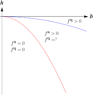
Here we investigate the phase diagram of the model : in the plane $(b,h)$, we prove that the quenched critical line (separating the phases of positive and zero free energy) lies strictly below the line $h=0$. Thus there exists a non trivial region where the field is localized though repulsed on average by the environment.

2 Results

We define the quenched (resp. annealed) free energy per site in $\Lambda\Subset\mathbb{Z}^{d}$ by :

$$f^{\mathbf{q}}_{\Lambda}(\mathbf{e})=|\Lambda|^{-1}\log\left(\frac{Z_{\Lambda}^{\mathbf{e},0}}{Z_{\Lambda}^{0,0}}\right),\quad f_{{\Lambda}}^{\mathbf{a}}(\mathbf{e})=|\Lambda|^{-1}\log\left(\frac{\mathbb{E}Z_{\Lambda}^{\mathbf{e},0}}{Z_{\Lambda}^{0,0}}\right),$$ (3)

where $Z_{\Lambda}^{0,0}$ denotes the partition function of the model with no potential, $e_{x}\equiv 0$ (i.e. of the Gaussian free field). In the case when $\Lambda=\Lambda_{n}=\{0,...,n-1\}^{d}$ we will use short forms $f^{\mathbf{q}}_{n}(\mathbf{e})$ and $f^{\mathbf{a}}_{n}(\mathbf{e})$. By the Jensen inequality, we have $f^{\mathbf{q}}(\mathbf{e})\leq f^{\mathbf{a}}(\mathbf{e})$. Moreover, it is not difficult to see that the annealed model corresponds to the model with constant (we will also say homogenous) pinning with the strength

$$\ell(\mathbf{e}):=\log(\mathbb{E}(e^{b\cdot e_{x}+h})).$$ (4)

for all $x\in\Lambda$. In other words $\mathbb{E}Z^{\mathbf{e},0}_{\Lambda}=Z^{\ell(\mathbf{e}),0}_{\Lambda}$.

In [4, Fact 2.3] we proved that for any environment $\mathbf{e}$ such that the annealed model exists, i.e. $\mathbb{E}(e^{b\cdot e_{x}+h})<\infty$, both the quenched and annealed free energies are non-negative. This motivates the following notions. We introduce the quenched (resp. annealed) critical lines, which are delimiting the region where $f^{\mathbf{q}}(\mathbf{e})=0$ (resp. $f^{\mathbf{a}}(\mathbf{e})=0$) from the region $f^{\mathbf{q}}(\mathbf{e})>0$ (resp. $f^{\mathbf{a}}(\mathbf{e})>0$).

$$h_{c}^{\mathbf{q}}(b):=\sup\{h\in\mathbb{R}:f^{\mathbf{q}}(\mathbf{e})=0\}\quad\mbox{ and }\quad{h}_{c}^{\mathbf{a}}(b):=\sup\{h\in\mathbb{R}:f^{\mathbf{a}}(\mathbf{e})=0\}$$

We are interested in describing the behavior of these quantities in the phase diagram described by the plane $(b,h)$. Knowing the behavior of the homogenous model for positive pinning [3], we easily deduce that the annealed critical line is given by the equation $\ell(\mathbf{e})=0$.
Note that $f^{\mathbf{q}}(\mathbf{e})\leq f^{\mathbf{a}}(\mathbf{e})$ implies that $h_{c}^{\mathbf{q}}(b)\geq{h}_{c}^{\mathbf{a}}(b).$ In Theorem 2.1 we show that the quenched critical line lies strictly below the axis $h=0$ in the neighborhood of $b=0$ for all $d\geq 2$. Our result shows in particular that there exists a non trivial region where $h<0$, $b>0$ and $f^{\mathbf{q}}(\mathbf{e})>0$, i.e.Β where the field is localized though it is repulsed on average by the environment.

Note that we don’t have any estimate on the behavior of $h_{c}^{\mathbf{q}}(b)-{h}_{c}^{\mathbf{a}}(b)$.

Theorem 2.1.

Let $\mathbf{e}\sim\otimes_{x\in\mathbb{Z}^{d}}\text{Bernoulli}_{1/2}(-1,+1)$. Then,

For $d\geq 2$, the quenched critical line is located in the quadrant $\{(b,h):b\geq 0,h<0\}$.

More precisely, there exists some $C,C^{\prime}>0$ depending on $d,a$ only and $\epsilon\in(0,1)$ such that for any environment $\mathbf{e}$ which fulfills $b+h>0$, $-\epsilon<-b+h<0$ and

$$\begin{cases}h>\frac{C^{\prime}(-b+h)^{2}}{\log(b-h)}&\mbox{ for }d=2\\ h>-C\cdot(-b+h)^{2}&\mbox{ for }d\geq 3,\end{cases}$$

we have $f^{\mathbf{q}}(\mathbf{e})>0$.

Remark 2.2.
  1. 1.

    A sketch of these bounds in the plane ($b,h$) can be seen on FigureΒ 1. Moreover, the bound for $d\geq 3$ can be rewritten as $h>-C^{\prime\prime}(d,a)\cdot b^{2}$.

  2. 2.

    Jensen’s inequality gives us an upper bound on $C,C^{\prime}$. Indeed, as $f^{\mathbf{a}}(\mathbf{e})\geq f^{\mathbf{q}}(\mathbf{e})$, if $f^{\mathbf{a}}(\mathbf{e})=0$ then $f^{\mathbf{q}}(\mathbf{e})=0$. In particular, we must have $-C\leq\frac{\partial^{2}}{\partial b^{2}}{h_{c}|}_{b=0}<0$. Our result gives thus an upper-bound on the behavior of the quenched critical line near $b=0$.

Refer to caption
Figure 1: (Color online) Phase diagram of the model. The red curve is the annealed critical line; the blue one is our bound on the quenched critical line.

2.1 Related results

The same type of result has been proven for (1$d$) polymer models in great generality in [1], where Alexander and Sidoravicius consider a polymer, with monomer locations modeled by the trajectory of a Markov chain $(X_{i})_{i\in\mathbb{Z}}$, in the presence of a potential (usually called a β€œdefect line”) that interacts with the polymer when it visits 0. Formally, the model is given by weighting the realization of the chain with the Boltzmann term

$$\exp\left(\beta\sum_{i=1}^{n}(u+V_{i})\mathbbm{1}_{\left[{X_{i}=0}\right]}\right).$$

with $(V_{i})_{i\in\mathbb{Z}}$ an i.i.d.Β sequence of 00-mean random variables. They studied the localization transition in this model. We say that the polymer is pinned, if a positive fraction of monomers is at 0. In the plane $(\beta,u)$ critical lines are defined as above: for $\beta$ fixed, $u_{c}^{\mathbf{q}}(\beta)$ (resp. $u_{c}^{\mathbf{a}}(\beta)$) is the value of $u$ above which the polymer is pinned with probability 1 (for the quenched (resp. annealed) measure). They showed that the quenched free energy and critical point are non-random, calculated the critical point for a deterministic interaction (i.e.Β Vi≑0subscript𝑉𝑖0V_{i}\equiv 0) and proved that the critical point in the quenched case is strictly smaller.

When the underlying chain is a symmetric simple random walk on $\mathbb{Z}$, the deterministic critical point is 00, so having the quenched critical point $u_{c}(\beta)$ strictly negative means that, even when the disorder is repulsive on average, the chain is pinned. This result was obtained by Galluccio and Graber in [7] for a periodic potential, which is frequently used in the physics literature as a β€œtoy model” for random environments.

A much shorter proof with explicit bounds can be found in [8], in less generality, but [6] contains a revisited proof with explicit estimates and weakening the assumptions on the underlying model.

Note that for polymers, or discrete height interfaces, one need a coarse graining procedure to achieve the proof. In our case, as we will see in the next section, we can shift the continuous interface where the environment is unfavorable, and this has a small cost in dimension $d\geq 3$. The procedure is a bit more complicated in dimension 2 and we have to localize the field before by introducing a small mass.

2.2 Proof of Theorem 2.1

2.2.1 Case $d\geq 3$

We assume $-b+h<0<b+h$ i.e.Β the environment is repulsive if $e_{x}=-1$ while it is attractive if $e_{x}=+1$.

The idea is to tilt the measure such that the field $\varphi$ is shifted up of an amount $s$ on the sites $x$ for which $b\cdot e_{x}+h<0$. In this way the shift of the field follows the environment. For some technical reasons, we need to work with the measure with boundary condition $a$, so perform two changes of measure (first one changing boundary condition and the second one to following the environment). Let $s>0$ (to be fixed later).

fΞ›nπͺ​(𝐞)=nβˆ’d​log⁑μΛn,𝐞,s0,a​(d​μΛn0,ad​μΛn,𝐞,s0,a​d​μΛn0,0d​μΛn0,a​exp⁑(βˆ‘xβˆˆΞ›n(bβ‹…ex+h)β€‹πŸ™[Ο†x∈[βˆ’a,a]])),subscriptsuperscript𝑓πͺsubscriptΞ›π‘›πžsuperscript𝑛𝑑subscriptsuperscriptπœ‡0π‘ŽsubscriptΞ›π‘›πžπ‘ dsuperscriptsubscriptπœ‡subscriptΛ𝑛0π‘Ždsubscriptsuperscriptπœ‡0π‘ŽsubscriptΞ›π‘›πžπ‘ dsuperscriptsubscriptπœ‡subscriptΛ𝑛00dsubscriptsuperscriptπœ‡0π‘ŽsubscriptΛ𝑛subscriptπ‘₯subscriptΛ𝑛⋅𝑏subscript𝑒π‘₯β„Žsubscript1delimited-[]subscriptπœ‘π‘₯π‘Žπ‘Žf^{\mathbf{q}}_{\Lambda_{n}}(\mathbf{e})=n^{-d}\log\mu^{0,a}_{\Lambda_{n},\mathbf{e},s}\left(\frac{\mathrm{d}{\mu_{\Lambda_{n}}^{0,a}}}{\mathrm{d}{\mu^{0,a}_{\Lambda_{n},\mathbf{e},s}}}\frac{\mathrm{d}{\mu_{\Lambda_{n}}^{0,0}}}{\mathrm{d}{\mu^{0,a}_{\Lambda_{n}}}}\exp\left(\sum_{x\in\Lambda_{n}}(b\cdot e_{x}+h)\mathbbm{1}_{\left[{\varphi_{x}\in[-a,a]}\right]}\right)\right),

where $\left({\varphi_{x}}\right)_{x\in\Lambda_{n}}$ under ΞΌΞ›n,𝐞,s0,asubscriptsuperscriptπœ‡0π‘ŽsubscriptΞ›π‘›πžπ‘ \mu^{0,a}_{\Lambda_{n},\mathbf{e},s} is distributed as $\left({\varphi_{x}+s\mathbbm{1}_{\left[{{(b\cdot e_{x}+h)<0}}\right]}}\right)_{x\in\Lambda_{n}}$ under $\mu^{0,a}_{\Lambda_{n}}$. More formally, introducing T𝐞,s:((Ο†x)xβˆˆΞ›n)↦(Ο†x+sβ€‹πŸ™[(bβ‹…ex+h)<0])xβˆˆΞ›n:subscriptπ‘‡πžπ‘ maps-tosubscriptsubscriptπœ‘π‘₯π‘₯subscriptΛ𝑛subscriptsubscriptπœ‘π‘₯𝑠subscript1delimited-[]⋅𝑏subscript𝑒π‘₯β„Ž0π‘₯subscriptΛ𝑛T_{\mathbf{e},s}:(\left({\varphi_{x}}\right)_{x\in\Lambda_{n}})\mapsto\left({\varphi_{x}+s\mathbbm{1}_{\left[{{(b\cdot e_{x}+h)<0}}\right]}}\right)_{x\in\Lambda_{n}}, we define ΞΌΞ›n,𝐞,s0,asubscriptsuperscriptπœ‡0π‘ŽsubscriptΞ›π‘›πžπ‘ \mu^{0,a}_{\Lambda_{n},\mathbf{e},s} as ΞΌΞ›n0,a∘T𝐞,sβˆ’1subscriptsuperscriptπœ‡0π‘ŽsubscriptΛ𝑛superscriptsubscriptπ‘‡πžπ‘ 1\mu^{0,a}_{\Lambda_{n}}\circ T_{\mathbf{e},s}^{-1}.
Using Jensen’s inequality, we get

$\displaystyle f_{\Lambda_{n}}^{\mathbf{q}}(\mathbf{e})$ $\displaystyle=$ nβˆ’d​log⁑[ΞΌΞ›n,𝐞,s0,a​exp⁑(βˆ‘xβˆˆΞ›n(bβ‹…ex+h)β€‹πŸ™[Ο†x∈[βˆ’a,a]]+log⁑d​μΛn0,ad​μΛn,𝐞,s0,a+log⁑d​μΛn0,0d​μΛn0,a)]superscript𝑛𝑑subscriptsuperscriptπœ‡0π‘ŽsubscriptΞ›π‘›πžπ‘ subscriptπ‘₯subscriptΛ𝑛⋅𝑏subscript𝑒π‘₯β„Žsubscript1delimited-[]subscriptπœ‘π‘₯π‘Žπ‘Ždsubscriptsuperscriptπœ‡0π‘ŽsubscriptΛ𝑛dsubscriptsuperscriptπœ‡0π‘ŽsubscriptΞ›π‘›πžπ‘ dsubscriptsuperscriptπœ‡00subscriptΛ𝑛dsubscriptsuperscriptπœ‡0π‘ŽsubscriptΛ𝑛\displaystyle n^{-d}\log\left[\mu^{0,a}_{\Lambda_{n},\mathbf{e},s}\exp\left(\sum_{x\in\Lambda_{n}}(b\cdot e_{x}+h)\mathbbm{1}_{\left[{\varphi_{x}\in[-a,a]}\right]}+\log\frac{\mathrm{d}{\mu^{0,a}_{\Lambda_{n}}}}{\mathrm{d}{\mu^{0,a}_{\Lambda_{n},\mathbf{e},s}}}+\log\frac{\mathrm{d}{\mu^{0,0}_{\Lambda_{n}}}}{\mathrm{d}{\mu^{0,a}_{\Lambda_{n}}}}\right)\right]
$\displaystyle\geq$ nβˆ’d​μΛn,𝐞,s0,a​(βˆ‘xβˆˆΞ›n(bβ‹…ex+h)β€‹πŸ™[Ο†x∈[βˆ’a,a]]+log⁑d​μΛn0,ad​μΛn,𝐞,s0,a⏟(1)+log⁑d​μΛn0,0d​μΛn0,a⏟(2))superscript𝑛𝑑subscriptsuperscriptπœ‡0π‘ŽsubscriptΞ›π‘›πžπ‘ subscriptπ‘₯subscriptΛ𝑛⋅𝑏subscript𝑒π‘₯β„Žsubscript1delimited-[]subscriptπœ‘π‘₯π‘Žπ‘Žsubscript⏟dsubscriptsuperscriptπœ‡0π‘ŽsubscriptΛ𝑛dsubscriptsuperscriptπœ‡0π‘ŽsubscriptΞ›π‘›πžπ‘ 1subscript⏟dsubscriptsuperscriptπœ‡00subscriptΛ𝑛dsubscriptsuperscriptπœ‡0π‘ŽsubscriptΛ𝑛2\displaystyle n^{-d}\mu^{0,a}_{\Lambda_{n},\mathbf{e},s}\left(\sum_{x\in\Lambda_{n}}(b\cdot e_{x}+h)\mathbbm{1}_{\left[{\varphi_{x}\in[-a,a]}\right]}+\underbrace{\log\frac{\mathrm{d}{\mu^{0,a}_{\Lambda_{n}}}}{\mathrm{d}{\mu^{0,a}_{\Lambda_{n},\mathbf{e},s}}}}_{(1)}+\underbrace{\log\frac{\mathrm{d}{\mu^{0,0}_{\Lambda_{n}}}}{\mathrm{d}{\mu^{0,a}_{\Lambda_{n}}}}}_{(2)}\right)

As ZΞ›n,𝐞,s0,0=ZΞ›n0,0subscriptsuperscript𝑍00subscriptΞ›π‘›πžπ‘ subscriptsuperscript𝑍00subscriptΛ𝑛Z^{0,0}_{\Lambda_{n},\mathbf{e},s}=Z^{0,0}_{\Lambda_{n}} (which follows by change of variables in the Gaussian integral), the first term can be written as

(1)=βˆ’14​dβ€‹βˆ‘{x,y}βˆ©Ξ›nβ‰ βˆ…x∼y(Ο†xβˆ’Ο†y)2βˆ’(Ο†^xβˆ’Ο†^y)2114𝑑subscriptπ‘₯𝑦subscriptΛ𝑛similar-toπ‘₯𝑦superscriptsubscriptπœ‘π‘₯subscriptπœ‘π‘¦2superscriptsubscript^πœ‘π‘₯subscript^πœ‘π‘¦2(1)=-\frac{1}{4d}\sum_{\begin{subarray}{c}\{x,y\}\cap\Lambda_{n}\neq\varnothing\\ x\sim y\end{subarray}}(\varphi_{x}-\varphi_{y})^{2}-(\hat{\varphi}_{x}-\hat{\varphi}_{y})^{2}

where $\hat{\varphi}_{x}:=\varphi_{x}+s\mathbbm{1}_{\left[{b\cdot e_{x}+h<0}\right]}$. Hence, using the definition of ΞΌΞ›n,𝐞,s0,asubscriptsuperscriptπœ‡0π‘ŽsubscriptΞ›π‘›πžπ‘ \mu^{0,a}_{\Lambda_{n},\mathbf{e},s},

nβˆ’d​μΛn,𝐞,s0,a​((1))superscript𝑛𝑑subscriptsuperscriptπœ‡0π‘ŽsubscriptΞ›π‘›πžπ‘ 1\displaystyle n^{-d}\mu^{0,a}_{\Lambda_{n},\mathbf{e},s}((1)) $\displaystyle=$ βˆ’nβˆ’d4​d​μΛn0,a​(βˆ‘{x,y}βˆ©Ξ›nβ‰ βˆ…x∼y(Ο†^xβˆ’Ο†^y)2βˆ’(Ο†xβˆ’Ο†y)2)superscript𝑛𝑑4𝑑subscriptsuperscriptπœ‡0π‘ŽsubscriptΛ𝑛subscriptπ‘₯𝑦subscriptΛ𝑛similar-toπ‘₯𝑦superscriptsubscript^πœ‘π‘₯subscript^πœ‘π‘¦2superscriptsubscriptπœ‘π‘₯subscriptπœ‘π‘¦2\displaystyle-\frac{n^{-d}}{4d}\mu^{0,a}_{\Lambda_{n}}\left(\sum_{\begin{subarray}{c}\{x,y\}\cap\Lambda_{n}\neq\varnothing\\ x\sim y\end{subarray}}(\hat{\varphi}_{x}-\hat{\varphi}_{y})^{2}-(\varphi_{x}-\varphi_{y})^{2}\right)
$\displaystyle=$ βˆ’s2​nβˆ’d4​dβ€‹βˆ‘{x,y}βˆ©Ξ›nβ‰ βˆ…x∼y(πŸ™[bβ‹…ex+h<0]βˆ’πŸ™[bβ‹…ey+h<0])2superscript𝑠2superscript𝑛𝑑4𝑑subscriptπ‘₯𝑦subscriptΛ𝑛similar-toπ‘₯𝑦superscriptsubscript1delimited-[]⋅𝑏subscript𝑒π‘₯β„Ž0subscript1delimited-[]⋅𝑏subscriptπ‘’π‘¦β„Ž02\displaystyle-\frac{s^{2}n^{-d}}{4d}\sum_{\begin{subarray}{c}\{x,y\}\cap\Lambda_{n}\neq\varnothing\\ x\sim y\end{subarray}}(\mathbbm{1}_{\left[{b\cdot e_{x}+h<0}\right]}-\mathbbm{1}_{\left[{b\cdot e_{y}+h<0}\right]})^{2}

The second term contains only boundary contribution of order $n^{d-1}$. Indeed,

$$(2)=\left(2a\sum_{x\in\partial\Lambda_{n}}\varphi_{x}-a^{2}|\partial\Lambda_{n}|\right)+\log\left(\frac{Z^{0,a}_{\Lambda_{n}}}{Z^{0,0}_{\Lambda_{n}}}\right)\geq\left(2a\sum_{x\in\partial\Lambda_{n}}\varphi_{x}-a^{2}|\partial\Lambda_{n}|\right)-Cn^{d-1}$$

Hence,

nβˆ’d​μΛn,𝐞,s0,a​((2))β‰₯2​aβ‹…nβˆ’dβ€‹βˆ‘xβˆˆβˆ‚Ξ›nΞΌΞ›n0,a​(Ο†^x)βˆ’C​nβˆ’1β‰₯sβ€‹βˆ‘xβˆˆβˆ‚Ξ›nπŸ™[bβ‹…ex+h<0]βˆ’C​nβˆ’1β‰₯βˆ’C​nβˆ’1superscript𝑛𝑑subscriptsuperscriptπœ‡0π‘ŽsubscriptΞ›π‘›πžπ‘ 2β‹…2π‘Žsuperscript𝑛𝑑subscriptπ‘₯subscriptΛ𝑛subscriptsuperscriptπœ‡0π‘ŽsubscriptΛ𝑛subscript^πœ‘π‘₯𝐢superscript𝑛1𝑠subscriptπ‘₯subscriptΛ𝑛subscript1delimited-[]⋅𝑏subscript𝑒π‘₯β„Ž0𝐢superscript𝑛1𝐢superscript𝑛1n^{-d}\mu^{0,a}_{\Lambda_{n},\mathbf{e},s}((2))\geq{2a}\cdot{n^{-d}}\sum_{x\in\partial\Lambda_{n}}\mu^{0,a}_{\Lambda_{n}}(\hat{\varphi}_{x})-Cn^{-1}\geq s\sum_{x\in\partial\Lambda_{n}}\mathbbm{1}_{\left[{b\cdot e_{x}+h<0}\right]}-Cn^{-1}\geq-Cn^{-1}

We get

$\displaystyle f_{\Lambda_{n}}^{\mathbf{q}}(\mathbf{e})$ $\displaystyle\geq$ nβˆ’dβ€‹βˆ‘xβˆˆΞ›n(bβ‹…ex+h)​μΛn0,a​(Ο†^x∈[βˆ’a,a])βˆ’s2​nβˆ’d4​dβ€‹βˆ‘{x,y}βˆ©Ξ›nβ‰ βˆ…x∼y(πŸ™[bβ‹…ex+h<0]βˆ’πŸ™[bβ‹…ey+h<0])2βˆ’C​nβˆ’1superscript𝑛𝑑subscriptπ‘₯subscriptΛ𝑛⋅𝑏subscript𝑒π‘₯β„Žsubscriptsuperscriptπœ‡0π‘ŽsubscriptΛ𝑛subscript^πœ‘π‘₯π‘Žπ‘Žsuperscript𝑠2superscript𝑛𝑑4𝑑subscriptπ‘₯𝑦subscriptΛ𝑛similar-toπ‘₯𝑦superscriptsubscript1delimited-[]⋅𝑏subscript𝑒π‘₯β„Ž0subscript1delimited-[]⋅𝑏subscriptπ‘’π‘¦β„Ž02𝐢superscript𝑛1\displaystyle n^{-d}\sum_{x\in\Lambda_{n}}(b\cdot e_{x}+h)\mu^{0,a}_{{\Lambda_{n}}}(\hat{\varphi}_{x}\in[-a,a])-\frac{s^{2}n^{-d}}{4d}\sum_{\begin{subarray}{c}\{x,y\}\cap\Lambda_{n}\neq\varnothing\\ x\sim y\end{subarray}}(\mathbbm{1}_{\left[{b\cdot e_{x}+h<0}\right]}-\mathbbm{1}_{\left[{b\cdot e_{y}+h<0}\right]})^{2}-Cn^{-1}

Now we use the fact that the marginal laws of all $\varphi_{x}$, $x\in\Lambda_{n}$ under $\mu^{0,a}_{{\Lambda_{n}}}$ are Gaussian variables centered at $a$, i.e.Β Ο†xβˆΌπ’©β€‹(a,Οƒnx)similar-tosubscriptπœ‘π‘₯π’©π‘ŽsuperscriptsubscriptπœŽπ‘›π‘₯\varphi_{x}\sim\mathcal{N}(a,\sigma_{n}^{x}) where $\sigma_{n}^{x}=\mbox{Var}^{0,a}_{\Lambda_{n}}(\varphi_{x})\leq\mbox{Var}^{0,a}_{\infty}(\varphi_{x})\leq c(d)<\infty$ for $d\geq 3$. Therefore,

ΞΌΞ›n0,a​(Ο†x∈[βˆ’a,a])βˆ’ΞΌΞ›n0,a​(Ο†x+s∈[βˆ’a,a])subscriptsuperscriptπœ‡0π‘ŽsubscriptΛ𝑛subscriptπœ‘π‘₯π‘Žπ‘Žsubscriptsuperscriptπœ‡0π‘ŽsubscriptΛ𝑛subscriptπœ‘π‘₯π‘ π‘Žπ‘Ž\displaystyle\mu^{0,a}_{{\Lambda_{n}}}({\varphi_{x}\in[-a,a]})-\mu^{0,a}_{{\Lambda_{n}}}({\varphi_{x}+s\in[-a,a]}) $\displaystyle=$ ΞΌΞ›n0,0​(Ο†x∈[βˆ’2​a,0])βˆ’ΞΌΞ›n0,0​(Ο†x∈[βˆ’2​aβˆ’s,βˆ’s])subscriptsuperscriptπœ‡00subscriptΛ𝑛subscriptπœ‘π‘₯2π‘Ž0subscriptsuperscriptπœ‡00subscriptΛ𝑛subscriptπœ‘π‘₯2π‘Žπ‘ π‘ \displaystyle\mu^{0,0}_{{\Lambda_{n}}}({\varphi_{x}\in[-2a,0]})-\mu^{0,0}_{{\Lambda_{n}}}({\varphi_{x}\in[-2a-s,-s]}) (5)
$\displaystyle=$ C​(βˆ«βˆ’s0βˆ’βˆ«βˆ’2​aβˆ’sβˆ’2​a)​eβˆ’y2/2​σnx2​d​y𝐢superscriptsubscript𝑠0superscriptsubscript2π‘Žπ‘ 2π‘Žsuperscript𝑒superscript𝑦22superscriptsuperscriptsubscriptπœŽπ‘›π‘₯2𝑑𝑦\displaystyle C\left(\int_{-s}^{0}-\int_{-2a-s}^{-2a}\right)e^{-y^{2}/2{\sigma_{n}^{x}}^{2}}dy
$\displaystyle\asymp$ $\displaystyle s\quad\mbox{ as }n\to\infty,$

for $c(d)>>s$. In particular we will use that :

ΞΌΞ›n0,a​(Ο†x∈[βˆ’a,a])βˆ’ΞΌΞ›n0,a​(Ο†x+s∈[βˆ’a,a])subscriptsuperscriptπœ‡0π‘ŽsubscriptΛ𝑛subscriptπœ‘π‘₯π‘Žπ‘Žsubscriptsuperscriptπœ‡0π‘ŽsubscriptΛ𝑛subscriptπœ‘π‘₯π‘ π‘Žπ‘Ž\displaystyle\mu^{0,a}_{{\Lambda_{n}}}({\varphi_{x}\in[-a,a]})-\mu^{0,a}_{{\Lambda_{n}}}({\varphi_{x}+s\in[-a,a]}) $\displaystyle\geq$ C1​(d,a)β‹…s,β‹…subscript𝐢1π‘‘π‘Žπ‘ \displaystyle C_{1}(d,a)\cdot s,

for some $C_{1}(d,a)>0$.

$\displaystyle f_{n}^{\mathbf{q}}(\mathbf{e})\geq n^{-d}\sum_{x\in\Lambda_{n}}$ (bβ‹…ex+h)​(ΞΌΞ›n0,a​(Ο†x∈[βˆ’a,a])βˆ’C1​(d,a)​sβ€‹πŸ™[bβ‹…ex+h<0])⋅𝑏subscript𝑒π‘₯β„Žsubscriptsuperscriptπœ‡0π‘ŽsubscriptΛ𝑛subscriptπœ‘π‘₯π‘Žπ‘Žsubscript𝐢1π‘‘π‘Žπ‘ subscript1delimited-[]⋅𝑏subscript𝑒π‘₯β„Ž0\displaystyle(b\cdot e_{x}+h)\left(\mu^{0,a}_{\Lambda_{n}}(\varphi_{x}\in[-a,a])-C_{1}(d,a)s\mathbbm{1}_{\left[{b\cdot e_{x}+h<0}\right]}\right)
βˆ’s2​nβˆ’d4​dβ€‹βˆ‘{x,y}βˆ©Ξ›nβ‰ βˆ…x∼y(πŸ™[bβ‹…ex+h<0]βˆ’πŸ™[bβ‹…ey+h<0])2βˆ’C​nβˆ’1superscript𝑠2superscript𝑛𝑑4𝑑subscriptπ‘₯𝑦subscriptΛ𝑛similar-toπ‘₯𝑦superscriptsubscript1delimited-[]⋅𝑏subscript𝑒π‘₯β„Ž0subscript1delimited-[]⋅𝑏subscriptπ‘’π‘¦β„Ž02𝐢superscript𝑛1\displaystyle-\frac{s^{2}n^{-d}}{4d}\sum_{\begin{subarray}{c}\{x,y\}\cap\Lambda_{n}\neq\varnothing\\ x\sim y\end{subarray}}(\mathbbm{1}_{\left[{b\cdot e_{x}+h<0}\right]}-\mathbbm{1}_{\left[{b\cdot e_{y}+h<0}\right]})^{2}-Cn^{-1}

Observe that $\mu^{0,a}_{\Lambda_{n}}(\varphi_{x}\in[-a,a])=\mu^{0,0}_{\Lambda_{n}}(\varphi_{x}\in[-2a,0])\geq\mu^{0,0}_{\infty}(\varphi_{x}\in[-2a,0])\geq C_{2}(d,a)$ for some $C_{2}(d,a)>0$.

By taking the expectation with respect to the environment, using the bounded convergence theorem and the fact that $f^{\mathbf{q}}(\mathbf{e})=\mathbb{E}(f^{\mathbf{q}}(\mathbf{e}))$ (cf.[4, Theorem 2.1]) we get :

$\displaystyle f^{\mathbf{q}}(\mathbf{e})=\lim_{n\to\infty}\mathbb{E}f^{\mathbf{q}}_{\Lambda_{n}}(\mathbf{e})$ $\displaystyle\geq$ h​C2​(d,a)βˆ’s​C1​(d,a)2​(βˆ’b+h)βˆ’s216β„Žsubscript𝐢2π‘‘π‘Žπ‘ subscript𝐢1π‘‘π‘Ž2π‘β„Žsuperscript𝑠216\displaystyle hC_{2}(d,a)-\frac{sC_{1}(d,a)}{2}(-b+h)-\frac{s^{2}}{16} (6)

We may optimize over $s$ as the left hand side does not depend on it. Doing this one checks that $f^{\mathbf{q}}(\mathbf{e})>0$ as soon as

$$h>-\frac{C_{1}(d,a)}{C_{2}(d,a)}\cdot(-b+h)^{2}=:-K(d,a)\cdot(-b+h)^{2}$$

This gives the implicit equation in terms of the variance $b^{2}$ of $b\cdot e_{x}+h$ :

$\displaystyle h>b-\frac{1}{2K}+\frac{1}{2}\sqrt{\frac{1}{K^{2}}-\frac{8b}{K}}=-Kb^{2}+O(b^{3})$

The annealed critical curve as well as this bound are drawn on Figure 1. We recall that (5) is valid under assumption that $s$ is small. The maximum of (6) is realized at $s_{\max}=-4C_{1}\cdot(-b+h)$, thus it is enough to assume that $(-b+h)$ is small. ∎

2.2.2 Case $d=2$

In the case $d=2$, the variance of the Gaussian free field diverges with the size of the box, so we cannot use the previous estimates. To circumvent this problem we introduce the so-called massive free field. Let $m>0$,

$${\boldsymbol{\mu}}^{0,\zeta}_{{\Lambda_{n}},m}(d{\varphi})=\frac{1}{{\mathbf{Z}}_{{\Lambda_{n}},m}^{0,\zeta}}\exp\left(-\mathcal{H}_{\Lambda_{n}}(\varphi)-m^{2}\sum_{x\in\Lambda_{n}}(\varphi_{x}-\zeta)^{2}\right)\prod_{x\in\Lambda_{n}}d{\varphi_{x}}\prod_{x\in\partial\Lambda_{n}}\delta_{0}(d{\varphi_{x}}),$$ (7)

where $\mathcal{H}_{\Lambda}(\varphi)$ is defined in (2). Known facts about this model can be found in [5, Section 3.3]. In particular, the random walk representation for the massless GFF [3, (1.3)] is still true, but for a random walk $Y_{t}$ that is killed with rate $\xi(m)=\frac{m^{2}}{1+m^{2}}$, namely at each time $\ell$, if the walk has not already been killed, it is killed with probability $\xi(m)$, where the killing is independent of the walk. We write its law $P_{x}$ when it starts at $x$.

Lemma 2.3.

Let $d=2$. Then,

  1. 1.

    There exists some $C_{1}>0$ such that for $n$ large enough, $m>0$ small enough and all $x\in\Lambda_{n}$,

    $${\boldsymbol{\mu}}^{0,0}_{{\Lambda_{n}},m}(\varphi^{2}_{x})\leq C_{1}|\log(m)|.$$
  2. 2.

    There exists some $C_{2}>0$ such that for $n$ large enough and $m>0$ small enough, we have

    $$n^{-2}\log\frac{{\mathbf{Z}}^{0,0}_{{\Lambda_{n}},m}}{Z^{0,0}_{{\Lambda_{n}}}}\geq-C_{2}m^{2}|\log(m)|.$$
Proof.

These bounds are rather standard. We give here the main steps of the proofs with some references. For the first claim, we use the random walk representation [5] to write

$${\boldsymbol{\mu}}^{0,0}_{{\Lambda_{n}},m}(\varphi_{x}^{2})=\sum_{\ell=0}^{\infty}P_{x}(Y_{\ell}=x\,,\,\tau_{\Lambda_{n}}\wedge\aleph>\ell)=\sum_{\ell=0}^{\infty}(1-\xi(m))^{\ell}P_{x}(Y_{\ell}=x\,,\,\tau_{\Lambda_{n}}>\ell)$$

where $\tau_{\Lambda_{n}}$ is the first exit time of $\Lambda_{n}$ and $\aleph$ is the killing time of the random walk $Y_{t}$. Hence,

$\displaystyle{\boldsymbol{\mu}}^{0,0}_{{\Lambda_{n}},m}(\varphi_{x}^{2})\leq{\boldsymbol{\mu}}^{0,0}_{{\Lambda_{n}},m}(\varphi_{0}^{2})\leq\sum_{\ell=1}^{\infty}(1-\xi(m))^{\ell}P_{0}(X_{\ell}=0)$ (8)

where $X_{\ell}$ is a simple random walk (without killing). The projections of $X_{\ell}$ onto the two coordinate axis are two independent $1-$dimensional random walks $X_{\ell}^{1}$ and $X_{\ell}^{2}$, then by Stirling formula,

$$P_{0}(X_{2\ell}=0)=(P_{0}(X_{2\ell}^{1}=0))^{2}=\left(\binom{2\ell}{\ell}2^{-2\ell}\right)^{2}=\frac{1}{\pi\ell}(1+o(1))\quad\mbox{ as }\ell\to\infty$$

The asymptotics of (8) for small $m$ gives the desired upper-bound.
To prove the second claim we use the representation of the partition function described in [2, p.542] (it applies to the massive GFF with an obvious modification). We denote by $\tilde{P}$ the coupling of a random walk $X_{n}$ and a killed random walk $Y_{n}$ such that $Y_{n}=X_{n}$ up to its killing time $\aleph$,

$\displaystyle|\Lambda_{n}|^{-1}\log\frac{Z_{{\Lambda_{n}}}^{0,0}}{{\mathbf{Z}}_{{\Lambda_{n}},m}^{0,0}}$ $\displaystyle=$ $\displaystyle|\Lambda_{n}|^{-1}\left(\frac{1}{2}\sum_{x\in\Lambda_{n}}\sum_{\ell=1}^{\infty}\frac{1}{2\ell}\left(\tilde{P}_{x}(X_{2\ell}=x,\tau_{\Lambda_{n}}>2\ell)-\tilde{P}_{x}(Y_{2\ell}=x,\tau_{\Lambda_{n}}\wedge\aleph>2\ell)\right)\right)$ (9)
$\displaystyle\leq$ $\displaystyle\frac{1}{2}\sum_{\ell=1}^{\infty}\frac{1}{2\ell}\left(\tilde{P}_{0}(X_{2\ell}=0,\tau_{\Lambda_{n}}>2\ell)-\tilde{P}_{0}(Y_{2\ell}=0,\tau_{\Lambda_{n}}\wedge\aleph>2\ell)\right)$
$\displaystyle=$ $\displaystyle\frac{1}{2}\sum_{\ell=1}^{\infty}\frac{1}{2\ell}\tilde{P}_{0}(X_{2\ell}=0,\tau_{\Lambda_{n}}>2\ell,\aleph\leq 2\ell)$
$\displaystyle\leq$ $\displaystyle\frac{1}{2}\sum_{\ell=1}^{\infty}\frac{1}{2\ell}\tilde{P}_{0}(X_{2\ell}=0)\left(1-(1-\xi(m))^{2\ell}\right)$

Using the same estimate as in (8), the asymptotics of (9) for small $m$ gives the desired upper-bound. ∎

The idea is to tilt the measure, as in the proof for $d\geq 3$, first to work with the massive measure, and second to follow the environment such that the field $\varphi$ is shifted up of an amount $s$ on the sites $x$ for which $b\cdot e_{x}+h<0$. For some technical reason, we need to work with the measure with boundary condition $a$, so we perform three changes of measure (first one for changing boundary condition, a second one for adding mass, and a third one for following the environment).
Let $s>0$ and $m>0$ to be fixed later.

fΞ›nπͺ​(𝐞)=nβˆ’2​log⁑μΛn0,0​(expβ€‹βˆ‘xβˆˆΞ›n(bβ‹…ex+h)β€‹πŸ™[Ο•x∈[βˆ’a,a]])=nβˆ’2log𝝁Λn,m,𝐞,s0,ΞΆ(exp(βˆ‘xβˆˆΞ›n(bβ‹…ex+h)πŸ™[Ο•x∈[βˆ’a,a]]+logd​μΛn0,0d​μΛn0,ΞΆ+logd​μΛn0,ΞΆd​𝝁Λn,m0,ΞΆ+logd​𝝁Λn,m0,ΞΆd​𝝁Λn,m,𝐞,s0,ΞΆ))subscriptsuperscript𝑓πͺsubscriptΞ›π‘›πžsuperscript𝑛2subscriptsuperscriptπœ‡00subscriptΛ𝑛subscriptπ‘₯subscriptΛ𝑛⋅𝑏subscript𝑒π‘₯β„Žsubscript1delimited-[]subscriptitalic-Ο•π‘₯π‘Žπ‘Žsuperscript𝑛2subscriptsuperscript𝝁0𝜁subscriptΞ›π‘›π‘šπžπ‘ subscriptπ‘₯subscriptΛ𝑛⋅𝑏subscript𝑒π‘₯β„Žsubscript1delimited-[]subscriptitalic-Ο•π‘₯π‘Žπ‘Ždsubscriptsuperscriptπœ‡00subscriptΛ𝑛dsubscriptsuperscriptπœ‡0𝜁subscriptΛ𝑛dsubscriptsuperscriptπœ‡0𝜁subscriptΛ𝑛dsubscriptsuperscript𝝁0𝜁subscriptΞ›π‘›π‘šdsubscriptsuperscript𝝁0𝜁subscriptΞ›π‘›π‘šdsubscriptsuperscript𝝁0𝜁subscriptΞ›π‘›π‘šπžπ‘ f^{\mathbf{q}}_{{\Lambda_{n}}}(\mathbf{e})=n^{-2}\log\mu^{0,0}_{\Lambda_{n}}\left(\exp\sum_{x\in\Lambda_{n}}(b\cdot e_{x}+h)\mathbbm{1}_{\left[{\phi_{x}\in[-a,a]}\right]}\right)\\ =n^{-2}\log{\boldsymbol{\mu}}^{0,\zeta}_{{\Lambda_{n}},m,\mathbf{e},s}\left(\exp\left(\sum_{x\in\Lambda_{n}}(b\cdot e_{x}+h)\mathbbm{1}_{\left[{\phi_{x}\in[-a,a]}\right]}\right.\right.\\ \left.\left.+\log\frac{\mathrm{d}\mu^{0,0}_{{\Lambda_{n}}}}{\mathrm{d}\mu^{0,\zeta}_{{\Lambda_{n}}}}+\log\frac{\mathrm{d}\mu^{0,\zeta}_{{\Lambda_{n}}}}{\mathrm{d}{\boldsymbol{\mu}}^{0,\zeta}_{{\Lambda_{n}},m}}+\log\frac{\mathrm{d}{\boldsymbol{\mu}}^{0,\zeta}_{{\Lambda_{n}},m}}{\mathrm{d}{\boldsymbol{\mu}}^{0,\zeta}_{{\Lambda_{n}},m,\mathbf{e},s}}\right)\right)

where $\left({\varphi_{x}}\right)_{x\in\Lambda_{n}}$ under 𝝁Λn,m,𝐞,s0,ΞΆsubscriptsuperscript𝝁0𝜁subscriptΞ›π‘›π‘šπžπ‘ {\boldsymbol{\mu}}^{0,\zeta}_{{\Lambda_{n}},m,\mathbf{e},s} is distributed as $\left({\varphi_{x}+s\mathbbm{1}_{\left[{{(b\cdot e_{x}+h)<0}}\right]}}\right)_{x\in\Lambda_{n}}$ under ${\boldsymbol{\mu}}^{0,\zeta}_{{\Lambda_{n}},m}$ ; more formally, introducing T𝐞,s:((Ο†x)xβˆˆΞ›n)↦(Ο†x+sβ€‹πŸ™[(bβ‹…ex+h)<0])xβˆˆΞ›n:subscriptπ‘‡πžπ‘ maps-tosubscriptsubscriptπœ‘π‘₯π‘₯subscriptΛ𝑛subscriptsubscriptπœ‘π‘₯𝑠subscript1delimited-[]⋅𝑏subscript𝑒π‘₯β„Ž0π‘₯subscriptΛ𝑛T_{\mathbf{e},s}:(\left({\varphi_{x}}\right)_{x\in\Lambda_{n}})\mapsto\left({\varphi_{x}+s\mathbbm{1}_{\left[{{(b\cdot e_{x}+h)<0}}\right]}}\right)_{x\in\Lambda_{n}}, we define 𝝁Λn,m,𝐞,s0,ΞΆsubscriptsuperscript𝝁0𝜁subscriptΞ›π‘›π‘šπžπ‘ {\boldsymbol{\mu}}^{0,\zeta}_{{\Lambda_{n}},m,\mathbf{e},s} as 𝝁Λn,m0,΢∘T𝐞,sβˆ’1subscriptsuperscript𝝁0𝜁subscriptΞ›π‘›π‘šsuperscriptsubscriptπ‘‡πžπ‘ 1{\boldsymbol{\mu}}^{0,\zeta}_{{\Lambda_{n}},m}\circ T_{\mathbf{e},s}^{-1}. Using Jensen’s inequality we get

$\displaystyle f^{\mathbf{q}}_{{\Lambda_{n}}}(\mathbf{e})$ $\displaystyle\geq$ nβˆ’2​𝝁Λn,m,𝐞,s0,΢​(βˆ‘xβˆˆΞ›n(bβ‹…ex+h)β€‹πŸ™[Ο†x∈[βˆ’a,a]]+log⁑d​μΛn0,0d​μΛn0,΢⏟(1)+log⁑d​μΛn0,ΞΆd​𝝁Λn,m0,΢⏟(2)+log⁑d​𝝁Λn,m0,ΞΆd​𝝁Λn,m,𝐞,s0,΢⏟(3))superscript𝑛2subscriptsuperscript𝝁0𝜁subscriptΞ›π‘›π‘šπžπ‘ subscriptπ‘₯subscriptΛ𝑛⋅𝑏subscript𝑒π‘₯β„Žsubscript1delimited-[]subscriptπœ‘π‘₯π‘Žπ‘Žsubscript⏟dsubscriptsuperscriptπœ‡00subscriptΛ𝑛dsubscriptsuperscriptπœ‡0𝜁subscriptΛ𝑛1subscript⏟dsubscriptsuperscriptπœ‡0𝜁subscriptΛ𝑛dsubscriptsuperscript𝝁0𝜁subscriptΞ›π‘›π‘š2subscript⏟dsubscriptsuperscript𝝁0𝜁subscriptΞ›π‘›π‘šdsubscriptsuperscript𝝁0𝜁subscriptΞ›π‘›π‘šπžπ‘ 3\displaystyle n^{-2}{\boldsymbol{\mu}}^{0,\zeta}_{{\Lambda_{n}},m,\mathbf{e},s}\left(\sum_{x\in\Lambda_{n}}(b\cdot e_{x}+h)\mathbbm{1}_{\left[{\varphi_{x}\in[-a,a]}\right]}+\underbrace{\log\frac{\mathrm{d}\mu^{0,0}_{{\Lambda_{n}}}}{\mathrm{d}\mu^{0,\zeta}_{{\Lambda_{n}}}}}_{(1)}+\underbrace{\log\frac{\mathrm{d}\mu^{0,\zeta}_{{\Lambda_{n}}}}{\mathrm{d}{\boldsymbol{\mu}}^{0,\zeta}_{{\Lambda_{n}},m}}}_{(2)}+\underbrace{\log\frac{\mathrm{d}{\boldsymbol{\mu}}^{0,\zeta}_{{\Lambda_{n}},m}}{\mathrm{d}{\boldsymbol{\mu}}^{0,\zeta}_{{\Lambda_{n}},m,\mathbf{e},s}}}_{(3)}\right)

As in the proof for $d\geq 3$, we have

nβˆ’2​𝝁Λn,m,𝐞,s0,΢​((1))β‰₯βˆ’C​nβˆ’1.superscript𝑛2subscriptsuperscript𝝁0𝜁subscriptΞ›π‘›π‘šπžπ‘ 1𝐢superscript𝑛1n^{-2}{\boldsymbol{\mu}}^{0,\zeta}_{{\Lambda_{n}},m,\mathbf{e},s}((1))\geq-Cn^{-1}.

By Lemma 2.3, we have $\frac{{\mathbf{Z}}^{0,\zeta}_{{\Lambda_{n}},m}}{Z^{0,\zeta}_{{\Lambda_{n}}}}=\frac{{\mathbf{Z}}^{0,\zeta}_{{\Lambda_{n}},m}}{{\mathbf{Z}}^{0,0}_{{\Lambda_{n}},m}}\frac{{\mathbf{Z}}^{0,0}_{{\Lambda_{n}},m}}{Z^{0,0}_{{\Lambda_{n}}}}\frac{Z^{0,0}_{{\Lambda_{n}}}}{Z^{0,\zeta}_{{\Lambda_{n}}}}\geq-Cn-C_{2}n^{2}m^{2}|\log m|$, and then

$$(2)=\log\left(\frac{{\mathbf{Z}}^{0,\zeta}_{{\Lambda_{n}},m}}{Z^{0,\zeta}_{\Lambda_{n}}}\right)+m^{2}\sum_{x\in\Lambda_{n}}\varphi_{x}^{2}\geq-Cn-C_{2}n^{2}m^{2}|\log m|+m^{2}\sum_{x\in\Lambda_{n}}\varphi_{x}^{2}$$

hence,

nβˆ’2​𝝁Λn,m,𝐞,s0,΢​((2))β‰₯βˆ’C​nβˆ’1βˆ’C2​m2​|log⁑m|.superscript𝑛2subscriptsuperscript𝝁0𝜁subscriptΞ›π‘›π‘šπžπ‘ 2𝐢superscript𝑛1subscript𝐢2superscriptπ‘š2π‘šn^{-2}{\boldsymbol{\mu}}^{0,\zeta}_{{\Lambda_{n}},m,\mathbf{e},s}((2))\geq-Cn^{-1}-C_{2}m^{2}|\log m|.

Finally, noticing that 𝐙Λn,m,𝐞,s0,ΞΆ=𝐙Λn,m0,ΞΆsubscriptsuperscript𝐙0𝜁subscriptΞ›π‘›π‘šπžπ‘ subscriptsuperscript𝐙0𝜁subscriptΞ›π‘›π‘š{\mathbf{Z}}^{0,\zeta}_{{\Lambda_{n}},m,\mathbf{e},s}={\mathbf{Z}}^{0,\zeta}_{{\Lambda_{n}},m} (just perform a change of variables in the Gaussian integral), we can compute the third term.

(3)=βˆ’18β€‹βˆ‘{x,y}βˆ©Ξ›nβ‰ βˆ…x∼y(Ο†xβˆ’Ο†y)2βˆ’(Ο†^xβˆ’Ο†^y)2βˆ’m2β€‹βˆ‘xβˆˆΞ›n(Ο†xβˆ’s)2βˆ’(Ο†^xβˆ’s)2318subscriptπ‘₯𝑦subscriptΛ𝑛similar-toπ‘₯𝑦superscriptsubscriptπœ‘π‘₯subscriptπœ‘π‘¦2superscriptsubscript^πœ‘π‘₯subscript^πœ‘π‘¦2superscriptπ‘š2subscriptπ‘₯subscriptΛ𝑛superscriptsubscriptπœ‘π‘₯𝑠2superscriptsubscript^πœ‘π‘₯𝑠2(3)=-\frac{1}{8}\sum_{\begin{subarray}{c}\{x,y\}\cap\Lambda_{n}\neq\varnothing\\ x\sim y\end{subarray}}(\varphi_{x}-\varphi_{y})^{2}-(\hat{\varphi}_{x}-\hat{\varphi}_{y})^{2}-m^{2}\sum_{x\in\Lambda_{n}}(\varphi_{x}-s)^{2}-(\hat{\varphi}_{x}-s)^{2}

where $\hat{\varphi}_{x}:=\varphi_{x}+s\mathbbm{1}_{\left[{b\cdot e_{x}+h<0}\right]}$. Now we will use the fact that the marginal laws of all $\varphi_{x}$, $x\in\Lambda_{n}$ under ${\boldsymbol{\mu}}^{0,\zeta}_{{\Lambda_{n}},m}$ are Gaussian variables, i.e.Β Ο†xβˆΌπ’©β€‹(ΞΌnx,Οƒnx2)similar-tosubscriptπœ‘π‘₯𝒩superscriptsubscriptπœ‡π‘›π‘₯superscriptsuperscriptsubscriptπœŽπ‘›π‘₯2\varphi_{x}\sim\mathcal{N}(\mu_{n}^{x},{\sigma_{n}^{x}}^{2}) where $\mu_{n}^{x}\approx\zeta$ except for $x$ close to the boundary of the box. Indeed, by the random walk representation of the mean, there is $C>0$ such that $|{\boldsymbol{\mu}}^{0,\zeta}_{\Lambda_{n},m}(\varphi_{x})-\zeta|\leq C(1+m^{2})^{-\|x-\partial\Lambda_{n}\|}$. Moreover, ${(\sigma_{n}^{x})}^{2}=\mbox{{V}ar}^{0,\zeta}_{{\Lambda_{n}},m}(\varphi_{x})\leq C_{1}|\log m|$. Using the definition of 𝝁Λn,m,𝐞,s0,ΞΆsubscriptsuperscript𝝁0𝜁subscriptΞ›π‘›π‘šπžπ‘ {\boldsymbol{\mu}}^{0,\zeta}_{{\Lambda_{n}},m,\mathbf{e},s}, and computing the terms as in the proof for $d\geq 3$,

nβˆ’2​𝝁Λn,m,𝐞,s0,΢​((3))superscript𝑛2subscriptsuperscript𝝁0𝜁subscriptΞ›π‘›π‘šπžπ‘ 3\displaystyle n^{-2}{\boldsymbol{\mu}}^{0,\zeta}_{{\Lambda_{n}},m,\mathbf{e},s}((3)) $\displaystyle\geq$ βˆ’s28​n2β€‹βˆ‘{x,y}βˆ©Ξ›nβ‰ βˆ…x∼y(πŸ™[bβ‹…ex+h<0]βˆ’πŸ™[bβ‹…ey+h<0])2βˆ’m2​s2n2β€‹βˆ‘xβˆˆΞ›nπŸ™[bβ‹…ex+h<0]+Cn.superscript𝑠28superscript𝑛2subscriptπ‘₯𝑦subscriptΛ𝑛similar-toπ‘₯𝑦superscriptsubscript1delimited-[]⋅𝑏subscript𝑒π‘₯β„Ž0subscript1delimited-[]⋅𝑏subscriptπ‘’π‘¦β„Ž02superscriptπ‘š2superscript𝑠2superscript𝑛2subscriptπ‘₯subscriptΛ𝑛subscript1delimited-[]⋅𝑏subscript𝑒π‘₯β„Ž0𝐢𝑛\displaystyle-\frac{s^{2}}{8n^{2}}\sum_{\begin{subarray}{c}\{x,y\}\cap\Lambda_{n}\neq\varnothing\\ x\sim y\end{subarray}}(\mathbbm{1}_{\left[{b\cdot e_{x}+h<0}\right]}-\mathbbm{1}_{\left[{b\cdot e_{y}+h<0}\right]})^{2}-\frac{m^{2}s^{2}}{n^{2}}\sum_{x\in\Lambda_{n}}\mathbbm{1}_{\left[{b\cdot e_{x}+h<0}\right]}+\frac{C}{n}.

We get, for $n$ large enough and $m$ small enough

$\displaystyle f_{\Lambda_{n}}^{\mathbf{q}}(\mathbf{e})$ $\displaystyle\geq$ nβˆ’2β€‹βˆ‘xβˆˆΞ›n(bβ‹…ex+h)​𝝁Λn,m0,΢​(Ο†^x∈[βˆ’a,a])βˆ’s28​n2β€‹βˆ‘{x,y}βˆ©Ξ›nβ‰ βˆ…x∼y(πŸ™[bβ‹…ex+h<0]βˆ’πŸ™[bβ‹…ey+h<0])2superscript𝑛2subscriptπ‘₯subscriptΛ𝑛⋅𝑏subscript𝑒π‘₯β„Žsubscriptsuperscript𝝁0𝜁subscriptΞ›π‘›π‘šsubscript^πœ‘π‘₯π‘Žπ‘Žsuperscript𝑠28superscript𝑛2subscriptπ‘₯𝑦subscriptΛ𝑛similar-toπ‘₯𝑦superscriptsubscript1delimited-[]⋅𝑏subscript𝑒π‘₯β„Ž0subscript1delimited-[]⋅𝑏subscriptπ‘’π‘¦β„Ž02\displaystyle n^{-2}\sum_{x\in\Lambda_{n}}(b\cdot e_{x}+h){\boldsymbol{\mu}}^{0,\zeta}_{{\Lambda_{n}},m}(\hat{\varphi}_{x}\in[-a,a])-\frac{s^{2}}{8n^{2}}\sum_{\begin{subarray}{c}\{x,y\}\cap\Lambda_{n}\neq\varnothing\\ x\sim y\end{subarray}}(\mathbbm{1}_{\left[{b\cdot e_{x}+h<0}\right]}-\mathbbm{1}_{\left[{b\cdot e_{y}+h<0}\right]})^{2}
$\displaystyle-\frac{m^{2}s^{2}}{n^{2}}\sum_{x\in\Lambda_{n}}\mathbbm{1}_{\left[{b\cdot e_{x}+h<0}\right]}-C^{\prime}m^{2}|\log m|-Cn^{-1},$

for some $C$ and $C^{\prime}>0$. Note that for $O(n^{2})$ sites $x$, we have

𝝁Λn,m0,΢​(Ο†x∈[βˆ’a,a])βˆ’πΞ›n,m0,΢​(Ο†x+s∈[βˆ’a,a])subscriptsuperscript𝝁0𝜁subscriptΞ›π‘›π‘šsubscriptπœ‘π‘₯π‘Žπ‘Žsubscriptsuperscript𝝁0𝜁subscriptΞ›π‘›π‘šsubscriptπœ‘π‘₯π‘ π‘Žπ‘Ž\displaystyle{\boldsymbol{\mu}}^{0,\zeta}_{{\Lambda_{n}},m}({\varphi_{x}\in[-a,a]})-{\boldsymbol{\mu}}^{0,\zeta}_{{\Lambda_{n}},m}({\varphi_{x}+s\in[-a,a]}) $\displaystyle\asymp$ Φ΢,b′​(a)β‹…sΒ as ​nβ†’βˆž,β†’β‹…subscriptsuperscriptΞ¦β€²πœπ‘π‘Žπ‘ Β as 𝑛\displaystyle\Phi^{\prime}_{\zeta,b}(a)\cdot s\quad\mbox{ as }n\to\infty, (10)

for $s<<a\leq\zeta=C_{1}|\log m|$, and $b=C_{1}|\log m|$. Above $\Phi_{\zeta,b}$ stands for the p.d.f. of the above Gaussian distribution with mean $\zeta$ and variance $b^{2}$. In particular, for a positive fraction of $x$ (close to 1) and $m$ sufficiently small, we have the upper bound :

𝝁Λn,m0,΢​(Ο†x∈[βˆ’a,a])βˆ’πΞ›n,m0,΢​(Ο†x+s∈[βˆ’a,a])subscriptsuperscript𝝁0𝜁subscriptΞ›π‘›π‘šsubscriptπœ‘π‘₯π‘Žπ‘Žsubscriptsuperscript𝝁0𝜁subscriptΞ›π‘›π‘šsubscriptπœ‘π‘₯π‘ π‘Žπ‘Ž\displaystyle{\boldsymbol{\mu}}^{0,\zeta}_{{\Lambda_{n}},m}({\varphi_{x}\in[-a,a]})-{\boldsymbol{\mu}}^{0,\zeta}_{{\Lambda_{n}},m}({\varphi_{x}+s\in[-a,a]}) $\displaystyle\geq$ C1​(a)|log⁑m|β‹…s,β‹…subscript𝐢1π‘Žπ‘šπ‘ \displaystyle\frac{C_{1}(a)}{|\log m|}\cdot s,

for some $C_{1}(a)>0$. Now we can compute :

$\displaystyle f_{\Lambda_{n}}^{\mathbf{q}}(\mathbf{e})$ $\displaystyle\geq$ nβˆ’2β€‹βˆ‘xβˆˆΞ›n(bβ‹…ex+h)​(𝝁Λn,m0,΢​(Ο†x∈[βˆ’a,a])βˆ’C1​(a)|log⁑m|​sβ€‹πŸ™[bβ‹…ex+h<0])superscript𝑛2subscriptπ‘₯subscriptΛ𝑛⋅𝑏subscript𝑒π‘₯β„Žsubscriptsuperscript𝝁0𝜁subscriptΞ›π‘›π‘šsubscriptπœ‘π‘₯π‘Žπ‘Žsubscript𝐢1π‘Žπ‘šπ‘ subscript1delimited-[]⋅𝑏subscript𝑒π‘₯β„Ž0\displaystyle n^{-2}\sum_{x\in\Lambda_{n}}(b\cdot e_{x}+h)({\boldsymbol{\mu}}^{0,\zeta}_{{\Lambda_{n}},m}(\varphi_{x}\in[-a,a])-\frac{C_{1}(a)}{|\log m|}s\mathbbm{1}_{\left[{b\cdot e_{x}+h<0}\right]})
βˆ’s28​n2β€‹βˆ‘{x,y}βˆ©Ξ›nβ‰ βˆ…x∼y(πŸ™[bβ‹…ex+h<0]βˆ’πŸ™[bβ‹…ey+h<0])2βˆ’m2​s2n2β€‹βˆ‘xβˆˆΞ›nπŸ™[bβ‹…ex+h<0]superscript𝑠28superscript𝑛2subscriptπ‘₯𝑦subscriptΛ𝑛similar-toπ‘₯𝑦superscriptsubscript1delimited-[]⋅𝑏subscript𝑒π‘₯β„Ž0subscript1delimited-[]⋅𝑏subscriptπ‘’π‘¦β„Ž02superscriptπ‘š2superscript𝑠2superscript𝑛2subscriptπ‘₯subscriptΛ𝑛subscript1delimited-[]⋅𝑏subscript𝑒π‘₯β„Ž0\displaystyle-\frac{s^{2}}{8n^{2}}\sum_{\begin{subarray}{c}\{x,y\}\cap\Lambda_{n}\neq\varnothing\\ x\sim y\end{subarray}}(\mathbbm{1}_{\left[{b\cdot e_{x}+h<0}\right]}-\mathbbm{1}_{\left[{b\cdot e_{y}+h<0}\right]})^{2}-\frac{m^{2}s^{2}}{n^{2}}\sum_{x\in\Lambda_{n}}\mathbbm{1}_{\left[{b\cdot e_{x}+h<0}\right]}
$\displaystyle-C^{\prime}m^{2}|\log m|-Cn^{-1}$

Observe that ${\boldsymbol{\mu}}^{0,\zeta}_{{\Lambda_{n}},m}(\varphi_{x}\in[-a,a])\geq 2a\cdot\Phi^{\prime}_{\zeta,b^{2}}(-a)=\frac{\tilde{C}_{1}(a)}{|\log m|}$ uniformly in $x\in\Lambda_{n}$. Let us take the expectation with respect to the environment, and use the bounded convergence theorem and [4, Theorem 2.1], we get :

$\displaystyle f^{\mathbf{q}}(\mathbf{e})=\lim_{n\to\infty}\mathbb{E}f^{\mathbf{q}}_{{\Lambda_{n}}}(\mathbf{e})$ $\displaystyle\geq$ h​C~1​(a)|log⁑m|βˆ’sβ‹…C1​(a)​(βˆ’b+h)2​|log⁑m|βˆ’s2​m22βˆ’s216βˆ’C′​m2​|log⁑m|.β„Žsubscript~𝐢1π‘Žπ‘šβ‹…π‘ subscript𝐢1π‘Žπ‘β„Ž2π‘šsuperscript𝑠2superscriptπ‘š22superscript𝑠216superscript𝐢′superscriptπ‘š2π‘š\displaystyle h\frac{\tilde{C}_{1}(a)}{|\log m|}-s\cdot\frac{C_{1}(a)(-b+h)}{2|\log m|}-\frac{s^{2}m^{2}}{2}-\frac{s^{2}}{16}-C^{\prime}m^{2}|\log m|. (11)

Our aim now is to show that the right hand side can be positive even when $h$ is negative. In the above expression s,mπ‘ π‘šs,m are free parameters which we may vary. However, we have to remember that both $s$ and $m$ need to be small enough, which makes standard optimization analysis cumbersome. We are going to show that there exists $C>0$ and $\epsilon>0$ such that for any $b,h$ such that $(-b+h)\in(-\epsilon,0)$ and

$$h:=C\frac{(-b+h)^{2}}{\log(-(-b+h))},$$

there exist small $s$ and $m$ such that the r.h.s.Β of (11) is positive. Notice that the result will imply that for any $h\geq C\frac{(-b+h)^{2}}{\log(-(-b+h))}$ the free energy is positive. Let us choose the value of $s$ which maximizes (11) for fixed $m$, i.e.

$$s=-\frac{C_{1}(a)(-b+h)}{(m^{2}+1/4)|\log(m)|}.$$ (12)

and for $m$ let us take

$$m^{2}=-k/(\log k)^{3},\text{ where }k:=-h\tilde{C}_{1}(a)/C^{\prime}.$$ (13)

One can verify that with the above choice of parameters both $s$ and $m$ are as small as we want. Let us first put (12) into the r.h.s.Β of (11) and obtain

$\displaystyle f^{\mathbf{q}}(\mathbf{e})$ $\displaystyle\geq$ $\displaystyle h\frac{\tilde{C}_{1}(a)}{|\log m|}+\frac{C_{1}(a)^{2}(-b+h)^{2}}{(m^{2}+1/4)(\log m)^{2}}-C^{\prime}m^{2}|\log m|.$

For $k$ and consequently $m$ small enough we have

$\displaystyle f^{\mathbf{q}}(\mathbf{e})$ $\displaystyle\geq$ $\displaystyle h\frac{\tilde{C}_{1}(a)}{|\log m|}+\frac{C_{1}(a)^{2}(-b+h)^{2}}{2(\log m)^{2}}-C^{\prime}m^{2}|\log m|.$

Further let us multiply both sides by $(\log m)^{2}$ and insert (13).

$\displaystyle f^{\mathbf{q}}(\mathbf{e})(\log m)^{2}$ $\displaystyle\geq$ $\displaystyle-h\tilde{C}_{1}(a)\log m+\frac{C_{1}(a)^{2}(-b+h)^{2}}{2}+C^{\prime}m^{2}(\log m)^{3}$
$\displaystyle=$ $\displaystyle-\frac{h\tilde{C}_{1}(a)}{2}(\log k-3\log(|\log k|))+\frac{C_{1}(a)^{2}(-b+h)^{2}}{2}-C^{\prime}\frac{k(\log k-3\log(|\log k|))^{3}}{8(\log k)^{3}}$
$\displaystyle=$ $\displaystyle-h\frac{\tilde{C}_{1}(a)}{2}\log(-h\tilde{C}_{1}(a)/C^{\prime})+\frac{C_{1}(a)^{2}(-b+h)^{2}}{2}+h\frac{\tilde{C}_{1}(a)}{8}+o(h)\quad\mbox{as}\quad|h|\to 0$

From the last claim it is straightforward to conclude existence of $C$ (sufficiently small) and $\epsilon$ with the properties described above.∎

Acknowledgements.

We would like to warmly acknowledge Yvan Velenik for introducing us to the topic. L.C.Β was partially supported by the Swiss National Foundation. P.M.Β was supported by a Sciex Fellowship grant no.Β 10.044.

References

  • [1] K.Β S. Alexander and V.Β Sidoravicius. Pinning of polymers and interfaces by random potentials. Ann. Appl. Probab., 16(2):636–669, 2006.
  • [2] E.Β Bolthausen and D.Β Ioffe. Harmonic crystal on the wall: a microscopic approach. Comm. Math. Phys., 187(3):523–566, 1997.
  • [3] E.Β Bolthausen and Y.Β Velenik. Critical behavior of the massless free field at the depinning transition. Comm. Math. Phys., 223(1):161–203, 2001.
  • [4] L.Β Coquille and P.Β MiΕ‚oΕ›. A note on the Gaussian Free Field with disordered pinning on $\mathbb{Z}^{d}$, $d\geq 2$. preprint, 2013.
  • [5] A.Β Dembo and T.Β Funaki. Lectures on probability theory and statistics, volume 1869 of Lecture Notes in Mathematics. Springer-Verlag, Berlin, 2005. Lectures from the 33rd Probability Summer School held in Saint-Flour, July 6–23, 2003, Edited by Jean Picard.
  • [6] F.Β den Hollander. Random polymers, volume 1974 of Lecture Notes in Mathematics. Springer-Verlag, Berlin, 2009. Lectures from the 37th Probability Summer School held in Saint-Flour, 2007.
  • [7] S.Β Galluccio and R.Β Graber. Depinning transition of a directed polymer by a periodic potential: A $d$-dimensional solution. Phys. Rev. E, 53:R5584–R5587, Jun 1996.
  • [8] G.Β Giacomin. Random polymer models. Imperial College Press, London, 2007.