Solubility of iron in metallic hydrogen and stability of dense cores in giant planets

Abstract

The formation of the giant planets in our solar system, and likely a majority of giant exoplanets, is most commonly explained by the accretion of nebular hydrogen and helium onto a large core of terrestrial-like composition. The fate of this core has important consequences for the evolution of the interior structure of the planet. It has recently been shown that $\mathrm{H}_{2}\mathrm{O}$, MgO and $\mathrm{SiO}_{2}$ dissolve in liquid metallic hydrogen at high temperature and pressure. In this study, we perform ab initio calculations to study the solubility of an innermost metallic core. We find dissolution of iron to be strongly favored above 2000 K over the entire pressure range (0.4-4 TPa) considered. We compare with and summarize the results for solubilities on other probable core constituents. The calculations imply that giant planet cores are in thermodynamic disequilibrium with surrounding layers, promoting erosion and redistribution of heavy elements. Differences in solubility behavior between iron and rock may influence evolution of interiors, particularly for Saturn-mass planets. Understanding the distribution of iron and other heavy elements in gas giants may be relevant in understanding mass-radius relationships, as well as deviations in transport properties from pure hydrogen-helium mixtures.

Despite recent advances in computational methods improving understanding of the hydrogen-helium dominated outer layers (McMahon et al., 2012; French et al., 2012; Militzer, 2013; Wilson & Militzer, 2010), knowledge of the deep interior structure of giant planets is limited. Determining the size of a dense central cores in a giant planet is dependent upon the model and equation of state used. Current observational evidence yields recent estimates for present day core mass of $\sim$0$-$10 (Guillot, 2005) and $\sim$14$-$18 (Militzer et al., 2008) Earth masses for Jupiter, and $\sim$9$-$22 (Guillot, 2005) Earth masses for Saturn. The Juno spacecraft, en route to Jupiter, will improve this constraint with more precise measurements of the giant’s gravitational field (Helled, 2011). Meanwhile, the density profiles of Neptune and Uranus allow non-unique solutions for the compositional structure for much of the interior (Guillot, 1999b, 2005).

It has long been suggested (Stevenson, 1982a, b), that a portion of this dense material might be redistributed in solution with hydrogen. As a result, erosion of a dense core would cause it to shrink over the lifetime of the planet. Possible consequences of this process are only beginning to be enumerated in evolutionary models (Chabrier & Baraffe, 2007; Leconte & Chabrier, 2012; Mirouh, 2012). The establishment of a gradient in concentration of a heavy dissolved component may change the nature of convection in a portion of the planets interior. This ‘double-diffusive’ is hypothesized to reduce the efficiency of heat transfer, thereby altering the thermal evolution of the planet. Comprehensive understanding of the process has been limited by the lack of knowledge of the solubility of various phases in metallic hydrogen, as well as poor understanding of the scaling of convective efficiency in the presence of competing gradients of composition and temperature. In this study, we address the first issue for iron metal.

As a result of continuing discoveries by Kepler (Borucki et al., 2010) and other exoplanet surveys, the number of confirmed planets has climbed to over 800, the majority of which are giants. This presents a growing sampling of planetary mass-radii relationships that will be fundamental to understanding the evolution of giant planet interiors. The range of mass-radius relationships observed for exoplanets exhibit variation beyond those in the solar system. In some cases, such as Corot-20b (Deleuil et al., 2011), the relationships may even defy explanation by simple structural models. Redistribution of dense core material lowers the heavy element content required to explain anomalously high observed densities.

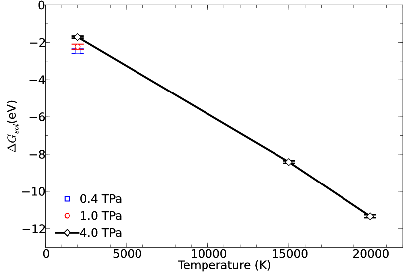
Figure 1: Gibbs free enerby of solvation for solid Fe in liquid metallic hydrogen. Negative values favor dissolution for a solute ratio of 1:256.

The favored model for gas giant formation (Mizuno et al., 1978; Bodenheimer & Pollack, 1986; Pollack et al., 1996) relies on the early formation of a large planetary embryo of critical mass to cause runaway accretion of hydrogen and helium gas. A competing theory involves collapse of a region of the disk under self-gravity, e.g. (Boss, 1997), but may have difficulty explaining significant enrichment of refractory elements (Hubbard et al., 2002; Guillot, 2005). The immediate result of a core-accretion hypothesis is a planet with the ice-rock-metal embryo residing at the center as a dense core, surrounded by an extensive layer of metallic hydrogen and helium. The role of core erosion to the subsequent evolution is a major source of uncertainty, but in principle, can explain shrinking of cores to masses smaller than those necessary to form the planet under the core-accretion hypothesis.

Core erosion in giant planets can be addressed by determining the solubility of analogous phases. Previous studies have considered an icy layer of fluid and superionic $\mathrm{H}_{2}\mathrm{O}$ (Wilson & Militzer, 2012a; Wilson et al., 2013), and a rocky layer consisting of MgO (Wilson & Militzer, 2012b) and $\mathrm{SiO}_{2}$ (Gonzalez et al., 2013), which have been shown to separate at relevant conditions (Umemoto, 2006). Assuming the same gross distribution, elements as terrestrial bodies, the innermost core component would be a dense, metallic alloy composed primarily of iron.

Ab initio random structure searches (Pickard & Needs, 2009) demonstrate that iron remains in a hexagonal close packed (hcp) structure remains stable up to pressures approaching Jupiter’s center, $\sim$2.3 TPa, at which point it undergoes a phase transition to face centered cubic (fcc) structure. (Stixrude, 2012) demonstrated a gradual decrease in this transition pressure with temperature. Simulations of liquid hydrogen (Militzer et al., 2008; Militzer, 2013; McMahon et al., 2012) undergo a gradual transition from molecular to metallic, which is complete by $\sim$ 0.4 TPa at low temperatures.

Table 1: Gibbs free energy of solvation for Fe in liquid H

(G$P$	($T$	Fe Phase	$\Delta G$
(GPa)	(K)	-	(eV)
400	2000	hcp	$-$2.2 $\pm$ 0.14
1000	2000	hcp	$-$2.5 $\pm$ 0.12
1000	2000	fcc	$-$2.3 $\pm$ 0.13
4000	2000	fcc	$-$1.71 $\pm$ 0.056
4000	15000	fcc	$-$8.42 $\pm$ 0.066
4000	20000	fcc	$-$11.34 $\pm$ 0.0780

Compression of materials with modern experimental techniques can reach megabar pressures, however the pressure-temperature conditions near Jupiter’s core ($>$4 TPa) remain inaccessible. Temperatures in shockwave experiments climb rapidly at high pressures in comparison with planetary adiabats, while diamond anvil cell experiments are best suited for low temperatures. As a result, simulations based on ab initio theories are best suited for directly probing the conditions of gas giant interiors.

We performed density functional theory molecular dynamics (DFT-MD) simulations to determine the energetics of a dissolution reaction, in which solid iron dissolves in pure liquid hydrogen. We calculate a Gibbs free energy of solvation:

$$\Delta G_{sol}\left(\mathrm{Fe}:256\mathrm{H}\right) = G\left(\mathrm{H}_{256}\mathrm{Fe}\right)$$

$$- \left[G\left(\mathrm{H}_{256}\right)+\frac{1}{32}G\left(\mathrm{Fe}_{32}\right)\right]\mathrm{,}$$

where $G\left(\mathrm{H}_{256}\right)$ and $G\left(\mathrm{Fe}_{32}\right)$ are the Gibbs free energies of a pure hydrogen liquid and solid or liquid iron. $G\left(\mathrm{H}_{256}\mathrm{Fe}\right)$ is the Gibbs free energy of 1:256 liquid solution of iron in hydrogen. We assume that analysis of a single low-concentration solution is sufficient to determine the onset of core erosion, since the reservoir of metallic hydrogen would be much larger than the core. This does not rule out non-ideal effects of higher concentrations that might exist in a narrow, poorly convecting layer at the top of a core.

Free energy calculations require the determination of a contribution from entropy, which is not determined from the standard DFT-MD formalism. To achieve this, we adopt a two step thermodynamic integration method, as used in previous studies (Morales et al., 2009; Wilson & Militzer, 2010, 2012a, 2012b). The method requires integration of the change in Helmholtz free energy over an unphysical, yet thermodynamically permissible, transformation between two systems governed by potentials $U_{a}\left(\mathbf{r_{i}}\right)$ and $U_{b}\left(\mathbf{r_{i}}\right)$. We define a hybrid potential $U_{\lambda}=\left(1-\lambda\right)U_{a}+\lambda U_{b}$, where $\lambda$ is the fraction of the potential $U_{b}\left(\mathbf{r_{i}}\right)$. The difference is Helmholtz free energy is then given by

$$\Delta F_{b\to a} \equiv F_{b}-F_{a}$$ (2a)

$$= \int_{0}^{1}{d\lambda\,\langle U_{b}\left(\mathbf{r_{i}}\right)-U_{a}\left(\mathbf{r_{i}}\right)\rangle_{\lambda}}$$ (2b)

where the averaging is over configurations generated during simulations of the system governed by the hybrid potential.

To increase the efficiency, we calculated the Helmholtz free energy in two steps each involving an integral of the form of Eq. 2. We first find $\Delta F_{\mathrm{DFT}\to\mathrm{cl}}$, between the systems governed by DFT and classical pair potentials, which are fit via a force-matching method (Izvekov et al., 2004). In the second step $\Delta F_{\mathrm{cl}\to\mathrm{an}}$, between the pair potentials and a reference system with an analytic solution $F_{\mathrm{an}}$. The Helmholtz energy for the DFT systems, $F_{\mathrm{DFT}}=F_{\mathrm{\mathrm{an}}}+\Delta F_{\mathrm{DFT}\to\mathrm{cl}}+\Delta F_{\mathrm{cl}\to\mathrm{an}}$, may then be compared directly. The first step requires DFT-MD simulations for a small number of $\lambda$ values, while the second uses applies a much faster classical Monte Carlo approach at numerous values of $\lambda$ to ensure a smooth integration.

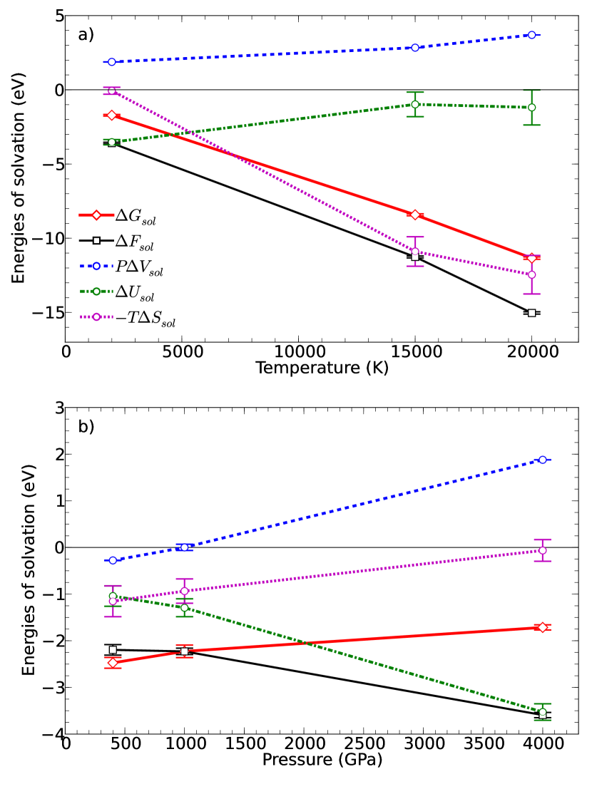
Figure 2: Breakdown of $\Delta G_{sol}$ into contributions from: internal energy, $\Delta U_{sol}$, pressure effects, $P\Delta V_{sol}$, and entropic effects, $-T\Delta S_{sol}$. Plots show variation with (a) temperature at P=4 TPa, and (b) pressure at T=2000 K.

Finding a suitable reference system is essential to the method, as it allows $\Delta F_{\mathrm{cl}\to\mathrm{DFT}}$ to be found with a small number of number of integration steps, and prevents solids from melting or transforming to a new structure. For liquid systems, we integrate to a non-interacting ideal gas, using classical two-body pair potentials as the intermediate step. For solid iron, we integrate to an Einstein solid, a system of non-interacting, 3-d harmonic oscillators. For the intermediate classical solid system we use a 50-50 ’mixture’ of two-body and one-body harmonic oscillator potentials. Spring constants for the Einstein terms are found from the mean-squared displacement of atoms from their ideal lattice sites during a DFT-MD simulation.

All simulations presented here were performed using the Vienna ab initio simulation package (VASP) (Kresse, 1996). VASP uses the DFT formalism utilizing pseudopotentials of the projector augmented wave type (Blochl, 1994) and the exchange-correlation functional of Perdew, Burke and Ernzerhof (Perdew et al., 1996). The iron pseudopotential treats a $[\mathrm{Mg}]\mathrm{3pd}^{6}\mathrm{4s}^{2}$ electron configuration as valence states, and a 2$\times$2$\times$2 grid of k-points is used for all simulations. Simulations on hydrogen and the solution were performed with a 900 eV cutoff energy for the plane wave expansion, while a 300 eV cutoff was used for iron. A time step of 0.2 fs was used for all liquid simulations, a 0.5$-$1.0 fs time step was used for high and low temperature iron simulations respectively. The $\Delta G_{sol}$ results were confirmed to be well-converged with respect to the energy cutoff and time step. Prohibitively long simulation times required that convergence with respect to finer k-point meshes be verified over a subset of configurations generated by a simulation with a 2$\times$2$\times$2 grid.

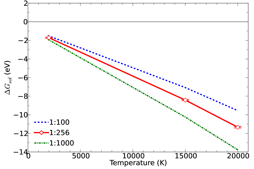
Figure 3: Shift in $\Delta G_{sol}$ from a system with and Fe:H ratio of 1:256 to 1:100 and 1:1000 in the low-concentration limit.

Iron simulations assume an hcp or fcc structure within their respective stability regimes (Pickard & Needs, 2009; Stixrude, 2012). We confirmed Fe to be solid up to 20000 K at 4 TPa, and to be a liquid at temperatures as low as 15000 K at 1 TPa. We also confirmed that the Gibbs free energy favors hcp stability over fcc at 1 TPa, though the difference is negligible for our subsequent analysis of dissolution. We found 32 atom supercells to be sufficient for Fe simulation. Finite size effects required that we use large 256 atom supercells for hydrogen, to which one Fe atom was added for the solution. Cubic supercells are used for fcc and liquid runs. In order to maintain the same number of atoms for the hcp an orthogonal supercell defined the combination of hexagonal unit cell vectors $\mathbf{a}$,$\mathbf{a}+\mathbf{b}$,and $\mathbf{c}$.

Cell volumes at each temperature were determined by fitting a pressure-volume polytrope equation of state to short DFT-MD simulations. The resulting DFT pressures were all within 0.1% of the target value. Gibbs free energies were computed for the three systems, $\mathrm{Fe}_{32}$, $\mathrm{H}_{256}$ and $\mathrm{H}_{256}\mathrm{Fe}_{1}$, using the thermodynamic integration method with simulation times of 1.0 ps for $\mathrm{H}_{256}$ and $\mathrm{H}_{256}\mathrm{Fe}_{1}$ and 2.5$-$5.0 ps for Fe. $\mathrm{H}_{256}$ and $\mathrm{H}_{256}\mathrm{Fe}_{1}$ runs with $\lambda=1$ were extended to 4.0 ns for precise calculations of the internal energy, which allows for determination of the entropic component of the Helmholtz free energy. The calculated energies and entropy are presented in Tab. I, along with the density. The Gibbs free energy of solvation, calculated using Eq. 1, is presented in Tab. II for each pressure-temperature condition. A negative $\Delta G_{sol}$ implies that the Gibbs free energy of the solution is lower than that of the separated phases. Therefore, dissolution is favored at a solute concentration higher than 1:256.

We find dissolution of iron to be strongly favorable at conditions corresponding to the interiors of gas giants. Fig. 1 shows the variation of $\Delta G_{sol}$ with temperature and pressure. $\Delta G_{sol}$ exceeds $-$10 eV per iron atom for plausible temperatures of Jupiter’s core. Dissolution remains favorable even at temperatures far below those predicted by model adiabats (Militzer, 2013; Militzer & Hubbard, 2013). The energetics are only weakly dependent on pressure, and $\Delta G_{sol}$ becomes increasingly negative with decreasing pressure. The solubility increases with a nearly linear trend in T, yielding slope of $\sim$0.53 meV/K. As a result, solubility is favored through the entire range of conditions considered, and likely the entire range for metallic hydrogen regions of giant planets.

Fig. 2 shows a breakdown of the data into contributions by various thermodynamic parameters. Included in the figure are: $\Delta F_{sol}$, $\Delta U_{sol}$, $P\Delta V_{sol}$ and $-T\Delta S_{sol}$, respectively, the Helmholtz free energy, internal energy, volumetric work and entropic contributions contributions to $\Delta G_{sol}$. Note that $\Delta F_{sol}$, $\Delta U_{sol}$ and $P\Delta V_{sol}$ are calculated independently, while $\Delta G_{sol}=\Delta F_{sol}+P\Delta V_{sol}$ and $-T\Delta S_{sol}=\Delta F_{sol}-\Delta U_{sol}$ are derived. The trend of solubility with temperature is dominated by the entropic term. The high solubility at low temperatures is reflected in the negative values of $\Delta U_{sol}$, indicating that the mixed system is energetically favorable independently of the entropy term.

Our calculations neglect any interactions between iron atoms in solution, and thus represent solubility in the low-concentration limit. $\Delta G_{sol}$ can be related to the volume change associated with the insertion of an iron of atom into hydrogen, as other contributions are constant with respect concentration. It can be shown that results for simulations with a 1:n solute ratio can be generalized to a ratio of 1:m using

$$\Delta G_{c} \approx F_{0}(H_{m}Fe)-F_{0}(H_{m})-F_{0}(Fe)$$

$$-\left[F_{0}(H_{m}Fe)-F_{0}(H_{m})-F_{0}(Fe)\right]$$

$$-\frac{\Delta G_{c}}{k_{B}T} \approx \log\left\{\frac{\left[V(\mathrm{H}_{n}\mathrm{Fe})+\frac{m-n}{n}V(\mathrm{H}_{n})\right]^{m+1}}{\left[V(\mathrm{H}_{n})\frac{m}{n}\right]^{m}}\right\}$$ (3b)

$$-\log\left\{\frac{\left[V(\mathrm{H}_{n}\mathrm{Fe})\right]^{n+1}}{\left[V(\mathrm{H}_{n})\right]^{n}}\right\},$$

where $\Delta G_{c}=\Delta G_{sol}(1:m)-\Delta G_{sol}(1:n)$, and $V(\mathrm{H}_{n})$ and $V(\mathrm{H}_{n}\mathrm{Fe})$ are the volumes for the simulations of hydrogen and the solution respectively. Fig. 3 shows the shift of $\Delta G_{sol}$ at 4 TPa at Fe concentrations of 1:100 and 1:1000. $\Delta G_{sol}$ is decreased for higher concentrations, but not to an extent where dissolution would become disfavored. At 20000 K this difference between 1:100 and 1:256 is $<$2 eV per iron atom, and at 2000 K is smaller than uncertainty in calculated values of $\Delta G_{sol}$.

The nature of the Fe-H system poses additional numerical challenges compared to other solutes considered previously (Wilson & Militzer, 2010, 2012a, 2012b; Gonzalez et al., 2013). These can largely be attributed to the comparatively large change in volume and electron density associated with the insertion of an iron atom into metallic hydrogen. We found it more efficient to determine cell volumes by fitting an equation of state to a collection of MD simulations at constant volume, rather than performing extended constant pressure simulations. Finite size effects were also found to be more significant for the Fe-H system, due to iron’s relatively large volume and number of valence electrons. Fig. 4 shows the convergence of a difference in internal energy between H and H-Fe for MD simulations with 128, 256 and 512 hydrogen atoms. We find 256 hydrogen atoms to be necessary in contrast to the previous studies that required only 128. The convergence with k-point grid resolution is also slower than in previous studies, and presents the greatest uncertainty in this study. MD calculations with a 3$\times$3$\times$3 k-point grid are prohibitively expensive. An estimate of this error for the results presented here is obtained by evaluating the internal energy over configurations sampled from a MD trajectory with a 2$\times$2$\times$2 k-point grid.Fig. 5 shows this estimated correction of $\Delta G_{sol}$ for the k-point grid used. The shifts are on the order $\sim$1 eV per iron atom, but are consistently negative for both quantities, leading to dissolution being more favorable.

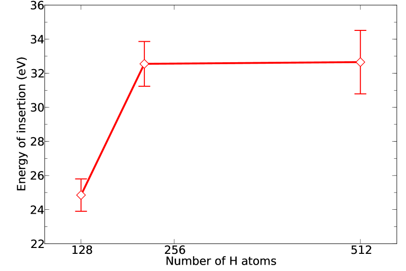
Figure 4: Energy of insertion for a single Fe atom into supercells containing 128, 256, and 512 atoms. Finite size effects are significant for $\mathrm{H}_{128}$, but are negligible within error for $\mathrm{H}_{256}$.

With the results of previous studies (Wilson & Militzer, 2012a, b; Gonzalez et al., 2013), we can now present a comprehensive picture for the solubility of all typical core materials in liquid metallic hydrogen. Dissolution is strongly favored for both iron and water ice. However, for water the high solubility is attributed entirely to the entropy, whereas iron has a favorable internal energy component that favors dissolution at low temperatures. Both phases are found to be soluble throughout the entire metallic hydrogen region of both Jupiter and Saturn. The rocky components, MgO and $\mathrm{SiO}_{2}$, have more moderate solubilities, with $\mathrm{SiO}_{2}$ being slightly higher. The saturation curves are, however, less steep than the adiabats for Jupiter and Saturn. As a result, solubility is favored for Jupiter’s core, but the rocky components of Saturn’s core may be stable given the present uncertainty in the planet’s adiabat.

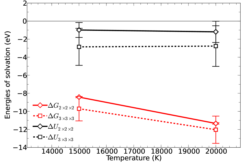
Figure 5: Estimated corrections to $\Delta G_{sol}$ and $\Delta G_{sol}$ coarseness of k-point grid used in DFT-MD runs. DFT calculations with a $3\times 3\times 3$ k-point grid were performed sampling a trajectory generated by an MD simulation with a $2\times 2\times 2$ k-point mesh.

The rocky components are found to be stable at lower pressures, approaching the metallic transition. If Mg and Si were convected upwards with sufficient concentration, they may precipitate, while Fe and $\mathrm{H}_{2}\mathrm{O}$ would remain in solution, at least to the molecular-metallic transition. The presence of a significant dissolved component at shallow depths may have consequences for the density profile and transport properties of hydrogen, which influence thermal structure and magnetic field generation.

Core erosion is thermodynamically favorable in gas giant planets, with the possible exception of smaller, cooler planets, like Saturn. For these planets, the outer icy layers are soluble, but the rocky layers may not be. The innermost iron component, though soluble, would be isolated from reaction with hydrogen. This might allow Saturn to have a larger, less eroded core than Jupiter, a result consistent with current observational constraints. Nevertheless, our results imply that confirmation of a massive core for Jupiter would support the core-accretion model over gravitational collapse. While erosion of such a core may be slow due to inefficient double-diffusive convection (Stevenson, 1982a; Chabrier & Baraffe, 2007; Leconte & Chabrier, 2012; Mirouh, 2012), settling of dispersed refractory material to form a core is inconsistent with our results. Late formation of a core would require a large amount material from captured planetesimals surviving descent to the planet’s center.

It may be possible to attribute some emerging trends in exoplanet mass-radius relationships to the difference in solubilities between rock and ice, or rock and metal. However, as we have shown, such thermodynamic differences are likely to only be significant in smaller, cooler planets, where redistribution of dense material by double-diffuse convection would be least efficient. The energetics of the dissolution reaction should be insignificant compared to the role of density in the redistribution of dense material. The work required to raise an iron of atom to the molecular-metallic transition is on the order of 1000 eV, whereas the contribution from the dissolution reaction is $\sim$1$-$10 eV. We conclude that the process of core erosion is thermodynamically consistent with ab initio simulations of the relevant materials, and its significance warrants close consideration in future models of giant planet evolution.

Table 2: Thermodynamic parameters derived from DFT-MD simulations.

P	T	System	Phase	$\rho$	F	U	G	S
(GPa)	(K)	-	-	($\mathrm{g}/\mathrm{cm}^{3}$)	(eV)	(eV)	(eV)	($\mathrm{k}_{b}/\mathrm{K}$)
400	2000	$\mathrm{Fe}_{32}$	hcp	14.408	$-$190.8(4)	$-$154.4(0)	323.3(4)	211.(4)
.	.	$\mathrm{H}_{256}$	liq	1.2709	$-$415.6(5)	$-$228.(0)	419.37(9)	1088.(2)
.	.	$\mathrm{H}_{256}\mathrm{Fe}$	liq	1.5192	$-$423.8(1)	$-$234.(0)	427.1(8)	1101.(6)
1000	2000	$\mathrm{Fe}_{32}$	hcp	18.279	$-$12.4(0)	18.1(2)	1000.8(5)	177.(1)
.	.	$\mathrm{H}_{256}$	liq	1.8916	23.0(3)	175.9(6)	1425.6(6)	887.(3)
.	.	$\mathrm{H}_{256}\mathrm{Fe}$	liq	2.2534	20.4(1)	175.(2)	1454.7(1)	898.(3)
1000	2000	$\mathrm{Fe}_{32}$	fcc	18.269	$-$10.35(0)	19.8(0)	1003.4(6)	174.(9)
.	.	$\mathrm{H}_{256}$	liq	1.8916	23.0(3)	175.9(6)	1425.6(6)	887.(3)
.	.	$\mathrm{H}_{256}\mathrm{Fe}$	liq	2.2534	20.4(1)	175.2(3)	1454.7(1)	898.(3)
4000	2000	$\mathrm{Fe}_{32}$	fcc	28.374	754.91(4)	777.6(2)	3365.97(1)	131.(8)
.	.	$\mathrm{H}_{256}$	liq	3.6375	1392.3(8)	1487.6(4)	4310.0(0)	552.(7)
.	.	$\mathrm{H}_{256}\mathrm{Fe}$	liq	4.3078	1412.3(8)	1508.(4)	4413.4(7)	55(7).(0)
4000	15000	$\mathrm{Fe}_{32}$	fcc	27.826	382.1(9)	87(5).0(0)	3045.7(0)	38(1).(0)
.	.	$\mathrm{H}_{256}$	liq	3.3618	$-$392.9(3)	1917.(3)	2763.9(8)	1787.(3)
.	.	$\mathrm{H}_{256}\mathrm{Fe}$	liq	3.9865	$-$392.2(5)	194(3).0(0)	2850.7(4)	1807.(2)
4000	20000	$\mathrm{Fe}_{32}$	fcc	27.550	176.(9)00	92(2).0(0)	2866.(8)00	43(2).(0)
.	.	$\mathrm{H}_{256}$	liq	3.2731	$-$1284.5(8)	208(1).0(0)	1957.2(6)	1952.(6)
.	.	$\mathrm{H}_{256}\mathrm{Fe}$	liq	3.8824	$-$1294.0(9)	210(4).0(0)	2035.5(1)	1972.(0)

References

- Blochl (1994) Blochl, P. E. 1994, Phys. Rev. B, 50, 17953.
- Bodenheimer & Pollack (1986) Bodenheimer, P., & Pollack, J. B. 1986, Icarus, 67, 391.
- Borucki et al. (2010) Borucki, W. J., Koch, D., Basri, G., Batalha, N., Brown, T., Caldwell, D., Caldwell, J., et al. 2010, Science, 327, 977.
- Boss (1997) Boss, A. P. 1997, Science, 276, 1836.
- Chabrier & Baraffe (2007) Chabrier, G., & Baraffe, I. 2007, ApJ, 661, L81.
- Deleuil et al. (2011) Deleuil, M., Bonomo, A. S., & Ferraz-Mello, S. 2011, A&A, 538, A145.
- French et al. (2012) French, M., Becker, A., Lorenzen, W., Nettelmann, N., Bethkenhagen, M., Wicht, J., & Redmer, R. 2012, ApJS, 202, 11p.
- Gonzalez et al. (2013) Gonzalez, F., Wilson, H. F., & Militzer, B. 2013, (in preparation).
- Guillot (1999a) Guillot, T. 1999a. Planet. Space Sci., 47, 1183.
- Guillot (1999b) Guillot, T. 1999b. Science, 286, 72.
- Guillot (2005) Guillot, T. 2005. Ann. Rev. Earth Planet. Sci., 33, 493.
- Helled (2011) Helled, R., & Anderson, J. D., Schubert, G., & Stevenson, D. J. 2011. Icarus, 216, 440.
- Hubbard et al. (2002) Hubbard, W. B., Burrows, A., & Lunine, J. I. 2002. ARA&A, 40, 103.
- Izvekov et al. (2004) Izvekov, S., Parrinello, M., Burnham, C. J., & Voth, G. A. 2004, J. Chem. Phys., 120, 10896.
- Kresse (1996) Kresse, G. 1996, Comp. Mater. Sci., 6, 15.
- Leconte & Chabrier (2012) Leconte, J., & Chabrier, G. 2012. A&A, 540, A20.
- McMahon et al. (2012) McMahon, J. M., Morales, M. A., Pierleoni, C., & Ceperley, D. M. 2012. Rev. Mod. Phys., 84, 1607.
- Militzer et al. (2008) Militzer, B., Hubbard, W. B., Vorberger, J., Tamblyn, I., & Bonev, S. A. 2008, ApJ, 688, L45.
- Militzer (2013) Militzer, B. 2013. Phys. Rev. B, 87, 014202.
- Militzer & Hubbard (2013) B. Militzer, & W. B. Hubbard, 2013. ApJ(in review).
- Mirouh (2012) Mirouh, G. M., Garaud, P., Stellmach, S., Traxler, a. L., & Wood, T. S. 2012. ApJ, 750, 18p.
- Mizuno et al. (1978) Mizuno, H., Nakazawa, K., & Hayashi, C. 1978. Prog. Theor. Phys., 60, 699.
- Morales et al. (2009) Morales, M. a, Schwegler, E., Ceperley, D., Pierleoni, C., Hamel, S., & Caspersen, K. 2009, PNAS, 106, 1324.
- Perdew et al. (1996) Perdew, J. P., Burke, K., & Ernzerhof, M. 1996, Phys. Rev. Lett., 77, 3865.
- Pickard & Needs (2009) Pickard, C. J., & Needs, R. J. 2009. J Phys-Condens Mat, 21, 452205.
- Pollack et al. (1996) Pollack, J. B., Hubicky, O., Bodenheimer, P., & Lissauer, J. J. 1996. Icarus, 124, 62.
- Stevenson (1982a) Stevenson, D. J. 1982a. Ann. Rev. Earth Planet. Sci., 10, 257.
- Stevenson (1982b) Stevenson, D. J. 1982b. Planet. Space Sci., 308, 755.
- Stixrude (2012) Stixrude, L. 2012. Phys. Rev. Lett., 108, 5p.
- Umemoto (2006) Umemoto, K., Wentzcovitch, R. M., & Allen, P. B. 2006. Science, 311, 5763, 983.
- Wilson & Militzer (2010) Wilson, Hugh F, & Militzer, B. 2010. Phys. Rev. Lett., 104, 12, 121101.
- Wilson & Militzer (2012a) Wilson, H. F., & Militzer, B. 2012. ApJ, 745, 54.
- Wilson & Militzer (2012b) Wilson, Hugh F., & Militzer, B. 2012. Phys. Rev. Lett., 108, 111101.
- Wilson et al. (2013) Wilson, H. F., Michael L. W, & B. Militzer, 2013. Phys. Rev. Lett.(in press).