Optical spectrum analyzer with quantum limited noise floor

Abstract

Interactions between atoms and lasers provide the potential for unprecedented control of quantum states. Fulfilling this potential requires detailed knowledge of frequency noise in optical oscillators with state-of-the-art stability. We demonstrate a technique that precisely measures the noise spectrum of an ultrastable laser using optical lattice-trapped ⁸⁷Sr atoms as a quantum projection noise-limited reference. We determine the laser noise spectrum from near DC to 100 Hz via the measured fluctuations in atomic excitation, guided by a simple and robust theory model. The noise spectrum yields a 26(4) mHz linewidth at a central frequency of 429 THz, corresponding to an optical quality factor of $1.6\times 10^{16}$. This approach improves upon optical heterodyne beats between two similar laser systems by providing information unique to a single laser, and complements the traditionally used Allan deviation which evaluates laser performance at relatively long time scales. We use this technique to verify the reduction of resonant noise in our ultrastable laser via feedback from an optical heterodyne beat. Finally, we show that knowledge of our laser’s spectrum allows us to accurately predict the laser-limited stability for optical atomic clocks.

The development of ultrastable frequency sources has paved the way for advances in fundamental tests of physics, primary frequency standards, precision spectroscopy, and quantum many-body systems. However, the utility of a precision frequency source is limited by its instabilities. For this reason, many methods to rigourously characterize these instabilities have been developed rutman78 . Ultrastable lasers pose a unique challenge to characterizing frequency instabilities because, until now, measurements of their performance required an optical herterodyne beat between two or more lasers young99 ; stoehr06 ; ludlow07 ; alnis08 ; dube09 ; jiang10 . Single laser performance can be inferred from a three-cornered hat measurement zhao09 ; kessler12 , but valuable information about a laser’s frequency noise power spectral density (PSD) cutler66 is limited in an optical beat by the less stable laser.

Optical lattice-trapped ⁸⁷Sr atoms are uniquely suited for laser noise spectral analysis due to the ultranarrow linewidth and field insensitivity of the ${}^{1}S_{0}$ $(\Ket{g})$ to ${}^{3}P_{0}$ $(\Ket{e})$ clock transition as well as the low quantum projection noise (QPN) achievable with ensembles of many atoms. To accomplish this, we adopt a technique similar to radio-frequency-based dynamical decoupling viola99 to manipulate the frequency noise sensitivity of this transition. Previous implementations of dynamical decoupling manipulated radio-frequency transitions in quantum systems to eliminate biercuk09 ; kotler11 or analyze bylander11 environmental noise. Here, the ⁸⁷Sr clock transition is so insensitive to perturbations that we are able to measure the noise spectrum of the ultrastable laser used to excited it. To guide and interpret our experimental measurements, we develop a simple and robust theoretical framework that combines concepts from rutman78 with a model for atomic sensitivity to frequency fluctuations dick87 ; santarelli98 ; quessada03 ; note1 . We compare experimentally measured fluctuations in atomic population to our theory and accurately determine the PSD of our laser. As laser stability advances, we can continue to leverage the QPN-limited noise floor of this technique to analyze lasers with greater stability.

To model the frequency of our laser, we consider a fixed frequency with a small, time-dependent noise term: $\omega_{L}(t)=\omega_{L_{0}}+\delta\omega(t)$. The instantaneous phase of the laser is given by $\phi_{L}(t)=\int_{0}^{t}dt^{\prime}\omega_{L}(t^{\prime})=\omega_{L_{0}}t+\int_{0}^{t}dt^{\prime}\delta\omega(t^{\prime})\equiv\omega_{L_{0}}t+\delta\phi(t)$. The resulting Hamiltonian for a two level atom, with energy spacing $\hbar\omega_{a}$, driven by this laser is sup

$$\frac{\hat{H}}{\hbar}=-\frac{\Omega(t)}{2}\left(\begin{array}[]{cc}0&e^{i\delta\phi(t)}\\ e^{-i\delta\phi(t)}&0\end{array}\right)-\frac{\overline{\Delta}}{2}\hat{\sigma}_{z},$$ (1)

where $\overline{\Delta}\equiv\omega_{L_{0}}-\omega_{a}$, $\hat{\sigma}_{z}$ is a Pauli spin matrix, and $\Omega(t)$ is the Rabi frequency. The chosen spectroscopy sequence determines the time dependence of $\Omega(t)$. In the absence of other perturbations, the atom-light interaction can be engineered to filter laser noise. For example, random fluctuations that occur on time scales that are fast compared to the atomic state evolution will average to zero.

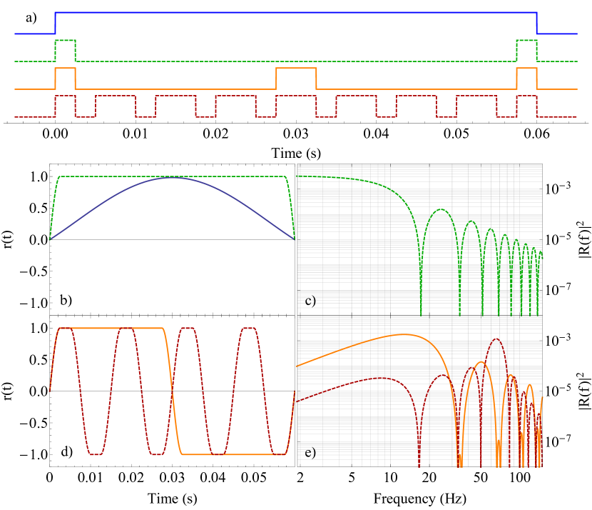
Figure 1: (color online) Schematic diagrams, $r(t)$, and $\left|R(f)\right|^{2}$ for different spectroscopy sequences. An example total spectroscopy time of 60 ms is shown. The schematic diagrams shown in (a) signify when $\Omega(t)$ is nonzero by their “high” value. For Rabi spectroscopy, the nonzero $\Omega$ is selected so the total pulse area is $\pi$ ($\pi$ pulse). For the other spectroscopy sequences, the nonzero value of $\Omega$ is $\pi/(0.005)$ rad/s. The diagrams are offset in height for clarity and are ordered top to bottom: Rabi, Ramsey, one-echo, and seven-echo.. Plots of $\left|R(f)\right|^{2}$ in (c) and (e) are calculated from the corresponding $r(t)$ curves plotted in (b) and (d). In (a), (b) and (c) solid blue (dashed green) lines correspond to Rabi (Ramsey) spectroscopy sequences. In (a), (d) and (e) solid orange (dashed red) lines correspond to one-echo (seven-echo) spectroscopy sequences.

To measure the effect of laser frequency fluctuation on the atoms, we observe fluctuations in the population imbalance between $\Ket{g}$ and $\Ket{e}$. For a general state $\Ket{\psi}=a\Ket{g}+b\Ket{e}$, the population imbalance is defined as $\mathbb{P}\equiv bb^{\ast}-aa^{\ast}$. We can express $\mathbb{P}$ in terms of the time-dependent laser detuning as

$$\mathbb{P}(\tau)=\mathbb{P}_{0}+\int_{0}^{\tau}dt\,r(t)\,\Delta(t),$$ (2)

where $\mathbb{P}_{0}$ is the initial imbalance, $\tau$ is the total spectroscopy time, $\Delta(t)\equiv\overline{\Delta}+\delta\omega(t)$, and $r(t)$ is the impulse response rutman78 , commonly referred to as the sensitivity function santarelli98 ; quessada03 . The sensitivity function, and its Fourier transform $R(f)$, are determined by the chosen spectroscopy sequence. As we apply different spectroscopy sequences, fluctuations in $\mathbb{P}$ correspondingly reveal laser instabilities at different Fourier frequencies, as illustrated by the shifting spectral response of $\left|R(f)\right|^{2}$ in Fig. 1(c) and 1(e).

Equation (2) rigorously connects $\mathbb{P}$ to $\Delta(t)$ and, to quantify fluctuations in $\mathbb{P}$, we consider its variance, $I^{2}\equiv\left\langle\mathbb{P}^{2}\right\rangle-\left\langle\mathbb{P}\right\rangle^{2}$, which can be expressed as sup

$$I^{2}=(2\pi)^{2}\int_{0}^{\infty}df\,S_{\nu}(f)\,\left|R(f)\right|^{2}.$$ (3)

Here, $S_{\nu}(f)$ is the single sided frequency noise PSD of the laser in units of Hz²/Hz. Figure 1 shows a schematic diagram for the spectroscopy sequences we use along with their corresponding sensitivity functions, $r(t)$ and $\left|R(f)\right|^{2}$.

For Rabi and Ramsey spectroscopy, the calculated value for $I$ diverges since thermal noise, a fundamental limit to $S_{\nu}(f)$ at low frequency, has an $f^{-1}$ character. For these measurements, we use the Allan deviation allan66 to characterize fluctuations in $\mathbb{P}$. In particular, we consider the two-sample Allan variance, defined as

$$I_{(2)}^{2}\equiv\frac{1}{2}\left\langle(\mathbb{P}_{i+1}-\mathbb{P}_{i})^{2}\right\rangle,$$ (4)

where the index $i$ signifies the $i$th measurement of $\mathbb{P}$. In the treatment of multiple measurements we consider the sensitivity function as periodic with a period equal to the experimental cycle time $T_{c}$. For this work, $T_{c}$ is approximately $1+\tau$ s. $I_{(2)}^{2}$ can also be expressed in terms of $S_{\nu}(f)$ as follows sup :

$$I_{(2)}^{2}=(2\pi)^{2}\int_{0}^{\infty}df\,S_{\nu}(f)\,2\sin^{2}(\pi fT_{c})\left|R(f)\right|^{2}.$$ (5)

Although the calculated value of $I_{(2)}$ remains finite for all experimental conditions, it does not properly account for coherent vibrational or electronic noise that exists on our laser at frequencies above 20 Hz. This noise is aliased onto our measurements and leads to regular, slow oscillations of the measured $\mathbb{P}$. To capture the effect of coherent noise, we use $I$ to characterize echo pulse sequences. Rabi and Ramsey sequences do not suffer from this aliasing because they do not have significant sensitivity to noise above 20 Hz for the spectroscopy times we use.

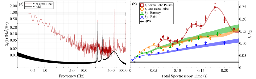
Figure 2: (color online) (a) $S_{\nu}(f)$ measured from a beat between the $\alpha$ and $\beta$ lasers is plotted in red. A model $S_{\nu}(f)$ for the $\alpha$ laser is plotted as a black band (see the text). (b) Measured values of $I$ or $I_{(2)}$ are plotted as a function of total spectroscopy time for the spectroscopy sequences shown in Fig. 1. Colored bands represent calculated values of $I$ or $I_{(2)}$ using the model $S_{\nu}(f)$ in (a) with QPN added in quadrature. A gray band indicates the mean calculated QPN for all experimental data. The black cross represents a measurement of the QPN (see the text).

Our experimental setup follows that of our Sr clock bishof11 ; campbell08 . Between 2000 and 3000 ⁸⁷Sr atoms are cooled to about 2 $\mathrm{\mu}$K in a one-dimensional optical lattice and nuclear spin polarized into the ground ${}^{1}S_{0}$ $m_{F}=9/2$ state. The optical lattice is kept near the magic wavelength ye08 for the $\Ket{g}$ to $\Ket{e}$ clock transition. Lattice-trapped atoms are excited with 698 nm light according to the spectroscopy sequences shown in Fig. 1(a). The clock light propagates along the strongly confined axis of the lattice so that it probes the atoms in the well-resolved sideband regime wineland98 ; blatt09 , free from Doppler and recoil effects. Finally, the numbers of atoms in $\Ket{g}$ and $\Ket{e}$ are measured to determine $\mathbb{P}$.

Using this setup, we have resolved 0.5 Hz spectral features swallows12 ; martin13 and demonstrated the most stable optical clock nicholson12 . These results are enabled by the ultrastable laser that addresses the clock transition (hereafter termed “$\alpha$ laser”). The stability of the $\alpha$ laser is at its thermal noise limit of $1\times 10^{-16}$ fractional frequency units for $\sim$1 to 1000 s. We can look for noise features at higher frequencies using an optical beat with a second laser (hereafter termed “$\beta$ laser”). The $\beta$ laser has demonstrated thermal noise-limited stability at the $10^{-15}$ fractional frequency level ludlow07 . The PSD of the optical beat (Fig. 2(a)) is limited by thermal noise in the $\beta$ laser out to Fourier frequencies of 10 Hz, beyond which it becomes limited by the noise floor of the detector; however, discrete features exist above this floor. Pairs of narrow noise peaks are visible near 22 and 30 Hz. Additionally, noise peaks are consistently measured at 24 and 60 Hz. The 60 Hz peak is dominated by detector noise and the 24 Hz peak is visible in previous beat measurements between two $\beta$ lasers ludlow07 .

Spectroscopy sequences are designed such that the measured $\mathbb{P}$ is sensitive to laser noise. For Rabi spectroscopy, we detune the $\alpha$ laser from resonance by the half width at half maximum (HWHM) of the Rabi line shape and apply a $\pi$ pulse. For Ramsey spectroscopy, we tune the laser exactly on resonance and apply two $\pi/2$ pulses separated in time. We shift the phase of the final $\pi/2$ pulse by $\pi/2$ radians relative to the initial $\pi/2$ pulse, which is equivalent to detuning by the HWHM of the central Ramsey fringe in the absence of phase shifts. The echo pulse sequences add to the Ramsey sequence a number of $\pi$ pulses such that the free evolution times between pulses are equal. We switch the phase of the laser by $\pi$ rad between adjacent echo pulses so that pulse area errors cancel. The echo pulse sequences act as a bandpass filter peaked at $(n+1)/(2\tau)$ Hz, where $n$ is the number of echo pulses. One can intuitively understand this behavior from the sensitivity functions in Fig. 1(d), which are periodic at this frequency. Figure 1(e) explicitly demonstrates this frequency sensitivity.

We use 80 consecutive measurements of $\mathbb{P}$ to estimate the raw standard(pair) deviation and its statistical uncertainty then divide by the measured contrast to get $I$($I_{(2)}$). The contrast is determined by a fit to the measured excitation versus detuning for Rabi spectroscopy or a fit to measured oscillations in excitation as the phase of the final pulse is scanned for other sequences. Figure 2(b) shows measured values of $I$ or $I_{(2)}$ for different spectroscopy sequences as a function of total spectroscopy time. Each data point represents a weighted mean of at least four measurements and error bars are estimated from the variance of the weighted mean. Spectroscopy times are investigated in a random order to avoid systematic drifts. Each data point consists of measurements separated by several hours to ensure consistency of the data.

The spectroscopy sequences we use are chosen to measure different Fourier components of $S_{\nu}(f)$ and demonstrate the utility of dynamical decoupling. The peak frequency sensitivity of the one-echo pulse data ranges between 5 and 50 Hz; however, individual noise components cannot be identified. By increasing the number of echo pulses to seven, we clearly resolve three peaks in the measured values of $I$, centered at 0.070, 0.135, and 0.180 s of total spectroscopy time. The peak centered at 0.135 s originates from alternating current motors in our lab operating near 30 Hz. The peak at 0.180 s corresponds to an acoustic resonance of the lab at 22 Hz. The width of the peak at 0.070 s corresponds to a frequency width that is broader than the resolution of the seven-echo pulse sequence (roughly $\tau^{-1}$). It contains multiple unresolved noise components corresponding to electrical noise at 60 Hz and acoustic noise near 40 and 80 Hz, which was previously observable in the optical heterodyne beat prior to the installation of an acoustic isolation box around the $\alpha$ laser. Lasers are also subject to white noise (no dependence on Fourier frequency) and noise proportional to $1/f$ originating from electronic and thermal noise respectively. At the magnitudes we extract from the experimental data, these noise components have a negligible effect on the calculated values of $I$ for seven-echo pulse sequences. In contrast, calculated values of $I_{(2)}$ for Rabi and Ramsey pulse sequences depend primarily on the magnitudes of white and $1/f$ noise since their $\left|R(f)\right|^{2}$ decreases with increasing $f$. The agreement between these two sequences is used to bound the uncertainty in the magnitudes of white and $1/f$ noise.

To determine $S_{\nu}(f)$ for the $\alpha$ laser we fit measured values of $I$ and $I_{(2)}$ to theoretical calculations using a single model $S_{\nu}(f)$ in Eqs. (3) and (5). The functional form of the model is

$$S_{\nu}(f)=h_{\mathrm{white}}+\frac{h_{\mathrm{thermal}}}{f}+\sum_{i=1}^{N}\frac{h_{i}}{1+\left(\frac{f-f_{i}}{\Gamma_{i}/2}\right)^{2}},$$ (6)

where $h_{i}$, $f_{i}$, and $\Gamma_{i}$ are the magnitude, frequency, and full width at half maximum (FWHM) for the $i^{th}$ noise resonance. All $h_{i}$ are fit to the seven-echo pulse data and the Rabi and Ramsey data are used to simultaneously fit $h_{\mathrm{white}}$ and $h_{\mathrm{thermal}}$. We determine $h_{\mathrm{thermal}}=1.5(4)\times 10^{-3}$ Hz², consistent with predicted thermal noise swallows12 , and $h_{\mathrm{white}}=3.3(3)\times 10^{-3}$ Hz${}^{2}/$Hz. Widths and frequencies of discrete noise peaks are chosen to be consistent with the optical beat. The parameters for these resonances are given in sup . We note that widths and frequencies could be identified without the aid of the optical beat, as demonstrated by the distinct peaks in Fig. 2(b), but the resolution would be limited to $\sim 1/\tau$. Although an exact relationship between $S_{\nu}(f)$ and a FWHM linewidth exists elliott82 , an analytic expression for this relationship does not exist with $1/f$ frequency noise. Here, the observed linewidth depends on the measurement time didomenico10 . By accounting for a finite measurement time, we numerically calculate the minimum observable $\alpha$ laser linewidth to be 26(4) mHz sup .

For each data point, the QPN is calculated for the measured number of atoms and the mean excitation fraction. The mean QPN for each sequence is added in quadrature with the calculated $I$ and $I_{(2)}$ to more accurately represent experimental data. These quantities are plotted as colored bands in Fig. 2(b) where the extent of the band corresponds to the uncertainty of the model $S_{\nu}(f)$. The mean and standard deviations of all calculated QPN values are represented in Fig. 2(b) as a gray band. QPN is experimentally measured by the standard deviation of $\mathbb{P}$ following a 5 ms, resonant, $\pi/2$ pulse. The measured and calculated QPN are consistent.

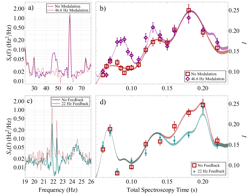
Figure 3: (color online) (a) Measured $S_{\nu}(f)$ of an optical beat between the $\alpha$ and $\beta$ lasers and (b) measured and calculated $I$ for seven-echo pulse sequences with and without modulation at 46.6 Hz. (c) Measured $S_{\nu}(f)$ of an optical beat between the $\alpha$ and $\beta$ lasers and (d) measured and calculated $I$ for seven-echo pulse sequences with and without feedback cancelation of 22 Hz noise. (d) Also demonstrated is the appearance of 60 Hz noise due to a malfunctioning signal generator that increases the measured $I$ at 0.06 and 0.2 s of total spectroscopy time.

To further test our theory we intentionally add noise to the $\alpha$ laser. White noise is passed through a bandpass filter at 46.6 Hz with 2 Hz bandwidth and used to frequency modulate the $\alpha$ laser with an acoustic optical modulator (AOM). Figure 3(a) demonstrates the effect of the modulation on the optical beat between the $\alpha$ and $\beta$ lasers. By adding noise into our model $S_{\nu}(f)$, corresponding to the 1st and 2nd order contributions of the modulation, we can fully account for measured values of $I$ with modulation. Figure 3(b) shows calculated and measured values of $I$ for seven-echo pulse spectroscopy with and without 46.6 Hz modulation.

In addition to using the optical beat to validate atomic measurements, we also harness the information within the beat to reduce discrete noise features in the $\alpha$ laser. We filter the beat with a bandpass at 22 Hz having subhertz bandwidth. This signal is inverted and fed back onto the $\alpha$ laser with an AOM. We can observe the effect of feedback on the beat (Fig. 3(c)), although we truly demonstrate the effectiveness of this technique by observing a reduction in $I$ for $\tau$ between 0.15 and 0.20 s when feedback is active (Fig. 3(d)). To reproduce the measured $I$ with feedback, the magnitude of 22 Hz noise needed to be reduced by 60% in the model $S_{\nu}(f)$ compared to the condition without feedback modulation.

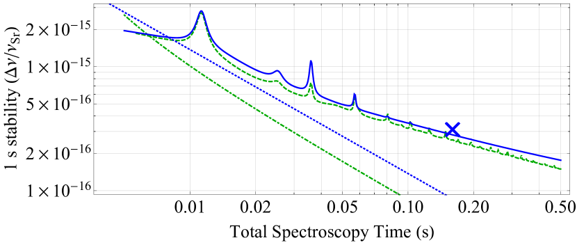
Figure 4: (Color online) The solid blue (dashed green) line represents the 1 s stability limit for an optical clock due to the Dick effect using Rabi (Ramsey) spectroscopy. The blue dotted (green dot-dashed) line represents the QPN stability limit at 1 s for Rabi (Ramsey) spectroscopy assuming a collection of 2000 uncorrelated atoms. Ramsey spectroscopy assumes 2.5 ms $\pi/2$ pulses. The blue “x” denotes the single clock 1 s stability from Ref. nicholson12 .

Having developed an accurate model for the $\alpha$ laser’s $S_{\nu}(f)$, we can predict the stability this laser can achieve when used in an optical atomic clock. Here, the laser’s frequency is slaved to the clock transition by periodic interrogation. The stability is limited by the Dick effect dick87 ; santarelli98 ; quessada03 , whereby periodic interrogation creates sensitivity to laser noise at harmonics of $1/T_{c}$. Figure 4, plots the one second stability limit due to the Dick effect for Rabi and Ramsey spectroscopy as a function of $\tau$, using the lower limit of the model $S_{\nu}(f)$. We assume a typical $T_{c}$ of $857.5+\tau$ ms. We find that for Rabi spectroscopy with $\tau=160$ ms, the Dick effect limits clock stability to $2.8\times 10^{-16}/\sqrt{\tau}$ in fractional frequency units. For a comparison of two uncorrelated clocks, one operating with 1000 atoms and one operating with 2000 atoms, we predict a stability of $4.6\times 10^{-16}/\sqrt{\tau}$ which is within $5\%$ of the achieved stability in Ref. nicholson12 .

We thank R. Ozeri for stimulating discussions on dynamical decoupling and J. K. Thompson and Z. Chen for parallel work and discussions on the treatment of oscillator phase noise in the Bloch vector picture chen12 . We thank T. L. Nicholson, B. J. Bloom, J. R. Williams, W. Zhang and S. L. Campbell for useful discussions. We acknowledge funding support for this work by DARPA QuASAR, NIST, and NSF.  M. B. acknowledges support from NDSEG.

References

- (1) J. Rutman, Proc. IEEE, 66, 1048 (1978).
- (2) B. C. Young, F. C. Cruz, W. M. Itano, and J. C. Bergquist, Phys. Rev. Lett. 82, 3799 (1999).
- (3) H. Stoehr, F. Mensing, J. Helmcke, and U. Sterr, Opt. Lett. 31, 736 (2006).
- (4) A. D. Ludlow et al., Opt. Lett. 32, 641 (2007).
- (5) J. Alnis, A. Matveev, N. Kolachevsky, Th. Udem, and T. W. Hänsch, Phys. Rev. A 77, 053809 (2008).
- (6) P. Dubé, A. A. Madej, J. E. Bernard, L. Marmet, and A. D. Shiner, Appl. Phys. B 95, 43 (2009).
- (7) Y. Y. Jiang et al., Nat. Photon. 5, 158 (2011).
- (8) Y. N. Zhao, J. Zhang, A Stejskal, T. Liu, V. Elman, Z. H. Lu, and L. J. Wang, Opt. Express 17, 8970 (2009).
- (9) T. Kessler et al., Nat. Photon. 6, 687 (2012).
- (10) L. S. Cutler, and C. L. Searle, Proc. IEEE, 54, 136 (1966).
- (11) L. Viola, E. Knill, and S. Lloyd, Phys. Rev. Lett. 82, 2417 (1999).
- (12) M. J. Biercuk, H. Uys, A. P. VanDevender, N Shiga, W. M. Itano, and J. J. Bollinger, Nature (London) 458, 996 (2009).
- (13) S. Kotler, N. Akerman, Y. Glickman, A. Keselman, and R. Ozeri, Nature (London) 473, 61 (2011).
- (14) J. Bylander et al., Nat. Physics 7, 565 (2011).
- (15) G. J. Dick, Proceedings of the 19th PTTI Applications and Planning Meeting, 1987 (U.S. Naval Observatory, Washington, D.C., 1988), p. 133.
- (16) G. Santarelli et al., IEEE Trans. Ultrason., Ferroelectr., Freq. Control 45, 887 (1998).
- (17) A. Quessada, R. P. Kovacich, I. Courtillot, A. Clairon, G. Santarelli, and P. Lemonde, J. Opt. B 5, S150 (2003).
- (18) We note that our treatment is consistent with that in chen12 .
- (19) See supplemental material for detailed derivations, calculations and technical comments.
- (20) D. W. Allan, Proc. IEEE, 54, 221 (1966).
- (21) M. Bishof et al., Phys. Rev. A 84, 052716 (2011).
- (22) G. K. Campbell et al., Metrologia 45, 539 (2008).
- (23) J. Ye, H. J. Kimble, and H. Katori, Science 320, 1734 (2008).
- (24) D. J. Wineland, et al., J. Res. Natl. Inst. Stand. Technol. 103, 259 (1998).
- (25) S. Blatt, et al., Phys. Rev. A 80, 052703 (2009).
- (26) M. D. Swallows et al., IEEE Trans. Ultrason., Ferroelectr., Freq. Control 59, 416 (2012).
- (27) M. J. Martin, M. Bishof, M. D. Swallows, X. Zhang. C. Benko, J. von-Stecher, A. V. Gorshkov, A. M. Rey, and J. Ye, arXiv:1212.6291.
- (28) T. L. Nicholson et al., Phys. Rev. Lett. 109, 230801 (2012).
- (29) D. S. Elliott, R. Roy, and S. J. Smith, Phys. Rev. A 26, 12 (1982).
- (30) G. Di Domenico, S. Schilt, and P. Thomann, Appl. Opt. 49, 4801 (2010).
- (31) Z. Chen, J. G. Bohnet, J. M. Weiner, and J. K. Thompson, Phys. Rev. A 86, 032313 (2012).