A Mechanism of Exciting Planetary Inclination and Eccentricity
through a Residual Gas Disk

Abstract

Accordling to the theory of Kozai resonance, the initial mutual inclination between a small body and a massive planet in an outer circular orbit is as high as $\sim 39.2^{\circ}$ for pumping the eccentricity of the inner small body. Here we show that, with the presence of a residual gas disk outside two planetary orbits, the inclination can be reduced as low as a few degrees. The presence of disk changes the nodal precession rates and directions of the planet orbits. At the place where the two planets achieve the same nodal processing rate, vertical secular resonance would occur so that mutual inclination of the two planets will be excited, which might trigger the Kozai resonance between the two planets further. However, in order to pump an inner Jupiter-like planet, the conditions required for the disk and the outer planet are relatively strict. We develop a set of evolution equations, which can fit the N-body simulation quite well but be integrated within a much shorter time. By scanning the parameter spaces using the evolution equations, we find that, a massive planet ($10M_{J}$) at $30$AU with $6^{o}$ inclined to a massive disk ($50M_{J}$) can finally enter the Kozai resonance with an inner Jupiter around the snowline. And a $20^{\circ}$ inclination of the outer planet is required for flipping the inner one to a retrograde orbit. In multiple planet systems, the mechanism can happen between two nonadjacent planets, or inspire a chain reaction among more than two planets. This mechanism could be the source of the observed giant planets in moderate eccentric and inclined orbits, or hot-Jupiters in close-in, retrograde orbits after tidal damping.

1 Introduction

Kozai mechanism is a kind of secular effect that occurred in hierarchical three-body systems(Lidov, 1962; Kozai, 1962; Naoz et al., 2011b). In the limit of circular restricted three-body model, the test particle in an inner orbit can be pumped to a highly eccentric or inclined orbit as long as its initial inclinations relative to the outer massive perturber is $\geq 39.2^{o}$(Kozai, 1962; Innanen et al., 1997). Further more, Lithwick & Naoz (2011) show that, when the massive perturber is in an eccentric orbit, the effect of octupole terms in the perturbing function will be effective so that the inner test particle may be repelled to retrograde orbits relative to the massive planet orbit.

One of the most prominent applications for Kozai mechanism is on the formation of orbital configurations for hot Jupiters (HJ). Recent observations of Rossiter-McLaughlin (RM) effect (Rossiter, 1924; McLaughlin, 1924) show that most of the HJs might be in orbits misaligned with stellar spins. Actually, for the 53 HJs with RM effect measurements, at least 8 HJs might be in retrograde motions(Winn et al., 2010; Triaud et al., 2010; Brown et al., 2012; Albrecht et al., 2012). As the classical core accretion scenario says that planets were formed in a protoplanetary disk surrounding the protostar, the existence of HJs in highly inclined orbits infers that some dynamical mechanisms to pump their inclinations must be exist after their formation. As the so-called disk migration scenario (Lin & Papaloizou, 1986; Lin et al., 1996) failed to explain the existence of HJs in retrograde orbits, Kozai mechnism was invoked to excite the orbital inclinations(Wu & Murray, 2003; Fabrycky & Tremaine, 2007; Naoz et al., 2011a; Nagasawa et al., 2008).

Wu & Murray (2003); Fabrycky & Tremaine (2007) proposed that a third massive body (either a binary or a brown dwarf companion) with a high orbital inclination($\geq 39.2^{\circ}$) can trigger the Kozai resonance so that the orbital eccentricity of inner planets can be pumped up to near 1, which can be damped at periastron of the orbit, with its excited inclination being preserved. However, the population studies establish that only $10\%$ of HJs can be explained by Kozai migration due to binary companions (Wu et al., 2007), while most of the HJ systems did not find any stellar or substellar companions. An alternative choice is whether the outer perturber can be replaced by a massive planet. Although this is possible, a very high mutual inclination between the two planets is required. E.g., Naoz et al. (2011a) presents a flipping example with a $3M_{J}$ planet as the outer perturber, while the initial mutual inclination of the two planets is up to $71.5^{\circ}$. Lithwick & Naoz (2011) shows that, if the outer perturbers are in more eccentric orbits, the relative inclination can be reduced, but still as high as $\sim 60^{o}$ for retrograde motion to be occurred. Thus, the origin of such high mutual inclination itself merits explanations.

In this paper, we propose a mechanism to efficiently excite planetary eccentricities and inclinations with an outer residual gas disk. After gas giants have formed and swept away the inner part of gas disk, the residual gas disk outside will perturb the architecture of inner planet systems. Due to the gravity of the residual disk, vertical secular resonances would occur between the very massive outer planet and the inner ones at some certain locations. Then the mutual inclination between the planetary orbits would be pumped. At this time, if the outer planet has a non-zero inclination relative to disk midplane, which might result from the previous planetary scattering, the mutual inclination is possible to raise up to the Kozai critical value, then the Kozai effect between planets would be induced. As a result, the eccentricities and inclinations of the inner planets would be excited to very high values.

The effect of gas disk in exciting planetary eccentricities was also studied by Nagasawa et al. (2003); Terquem et al. (2010); Teyssandier et al. (2012), etc. Our present work focus on how, with the aid of a disk, a two planet system will execute secular resonances between them in order to trigger the subsequent Kozai effect. We will also present the parameter studies with a set of evolution equations. The paper is organized as follows: in section 2, we introduce the model and two examples, and the pumping region is displayed by scanning the $a_{1,0}-I_{2,0}$ plane. Then we point out the pumping mechanism is the secular resonances coupled with the following Kozai resonance, and calculate the location of secular resonances in the situation of small eccentricities and inclinations by timescale comparisons in section 3. In section 4, we deduce the changing rates of some crucial parameters in pumping process relative to any inertial plane, and compare them with N-body simulation results. In section 5, influence of planetary parameters are investigated. According to that, we give the critical pumping conditions for a fixed gas disk. Section 6 displays situations in systems with more than two planets. Finally, discussions and conclusions are presented in section 7.

2 Model and Examples

We consider a planet system with two giant planets (denote as $m_{1}$ and $m_{2}$ for inner and outer planet, respectively) orbiting around a central star, with a protoplanetary disk whose inner part had been swept out by giant planets (Zhang et al., 2008; Zhang & Zhou, 2010a, b). The gas disk is assumed to be a two-dimensional circular annulus for simplicity, with its mass distributed on the midplane. As both the mass and the angular momentum of the disk are much larger than those of the planets, we further suppose the gravity of the planets has no influence on the disk, i.e., the disk is invariable. As the disk exerts the gravity onto the planets, the equation of planet motion can be written as follows

$$\frac{d^{2}\textit{{r}}_{i}}{dt^{2}}=-\frac{G(m_{0}+m_{i})}{r_{i}^{2}}\Bigg{(}\frac{\textit{{r}}_{i}}{r_{i}}\Bigg{)}+\sum_{j\neq i}^{N}Gm_{j}\Bigg{[}\frac{\textit{{r}}_{j}-\textit{{r}}_{i}}{|\textit{{r}}_{j}-\textit{{r}}_{i}|^{3}}-\frac{\textit{{r}}_{j}}{r_{j}^{3}}\Bigg{]}-\bigtriangledown\Phi,$$ (1)

where $\textit{{r}}_{i}$ is the position vector of the planets relative to the star, and

$$\Phi=-G\int_{R_{\rm in}}^{R_{\rm out}}\Sigma(r)rdr\int_{0}^{2\pi}\frac{d\phi}{(r^{2}+r_{p}^{2}-2rr_{p}\cos{\phi}\sin{\theta_{p}})^{1/2}}$$ (2)

displays the gravitational potential from the disk (Terquem et al., 2010). $R_{\rm in},R_{\rm out}$ is the inner and outer border of the disk. $(\alpha_{p},\varphi_{p},\theta_{p})$ is the spherical coordinates of a planet in the coordinate system settled by the star and the disk midplane. $\Sigma(r)$ is the mass density of the disk, and we use the most commonly exponential density distribution of the disk radius $r$, $\Sigma(r)=\Sigma_{0}(r/R_{\rm out})^{-\alpha}$. Total mass of the disk is settled by $M_{\rm disk}$ and the expression for $\Sigma_{0}$ is shown in Appendix B.

We apply Runge-Kutta-Fehlberg 7(8) integrator to integrate Equations (1). Figure 1 gives a typical example, whose initial conditions are listed in table 1. We set the star mass $m_{0}=1M_{\odot}$. The inner and outer boundary of the out gas disk are taken arbitrarily within the scope of disk observations. In order to satisfy the assumption that the angular momentum of the disk is overwhelming, we set the mass of the gas disk as $0.05M_{\odot}$. Though it is much larger than the average mass ($0.01M_{\odot}$) estimated by Williams & Cieza (2011), it is still within the reasonable range according to the recent transitional disk observation (such as LkCa 15 (Kraus & Ireland, 2012)). The mass of outer planet is moderately bigger than the inner one for facilitating the excitation procedure, and the particular influence will be discussed in section 5. We take the initial eccentricity and inclination of the inner planet very small just to show the pumping mechanism. Eccentricity of the outer planet is set very small in order to conveniently compare with the results of the evolution equations (section 4), and the non-zero eccentricity situation will be discussed in Section 5.

We can see from Figure 1 that the inclination of the inner planet relative to disk midplane ($I_{1}$) goes up to near $50^{\circ}$ within 0.3Myr. After around 0.4Myr, the eccentricity of the inner planet $e_{1}$ begins to rise, accompanied with the mutual inclination between planets ($I_{\rm tot}$) declining. Ascending nodes of the two planets precess with same rates for most of the first 0.3Myr, which implies that it is the secular resonance that raises $I_{1}$ and hence $I_{\rm tot}$. This triggers the whole excitation procedure. Argument of pericenter of the inner planet $\omega_{1}$ keeps librating during the cause. We also notice that for a while after 0.7Myr, $I_{1}$ becomes larger than $90^{\circ}$ and meanwhile $e_{1}$ is close to 1. It provides a good opportunity for the planet to turn into a retrograde hot-Jupiter after considering tidal damping due to the central star. As comparison, the case with the same initial conditions except for free of gas is shown in the right. Eccentricities from planetary secular perturbations merely are much smaller, and mutual inclination keeps around $30^{\circ}$ all the time.

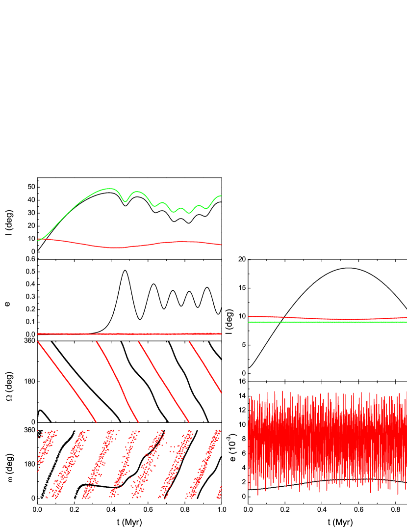
Figure 2: The same as Figure 1 except $a_{1,0}=5.5au,a_{2,0}=35.5au,I_{2,0}=10^{\circ}$.

Figure 2 gives another example with smaller initial inclination of $m_{2}$ ($I_{2,0}=10^{\circ}$)(The subscript 0 means the initial value, and hereafter). And the mutual inclination of two planets could also be stirred up to $40^{\circ}$ companied by the approaching nodes precession rates of the two planets. Then $e_{1}$ is pumped by Kozai effect with the sign of $\omega_{1}$ librating.

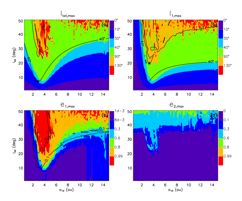
Figure 3: Contours of maximum of the mutual inclination between two planets $I_{\rm tot,max}$(a), maximum of the inclination of the inner planet $I_{\rm 1,max}$(b), maximum of the eccentricity of the inner planet $e_{\rm 1,max}$(c), maximum of the eccentricity of the outer planet $e_{\rm 2,max}$(d) from full N-body simulations during the evolution of 1Myr. Every point has different initial inclination of the outer planet $I_{2,0}$ ($y$ axis) and different initial semi-major axis of the inner planet $a_{1,0}$ ($x$ axis). The black lines in panel a,b and c indicate the results of the evolution equations (8), which are integrated 1 million years or truncated after $e_{1}>0.99$. The black stars in the two upper panels are used to label the positions whose coordinates are contoured in Figure 6.

The initial inclination $I_{2,0}$ and semi-major axes are critical parameters for pumping occurring, so we scanned the phase space of $a_{1,0}-I_{2,0}$, and for every case, extracted the maximum of $I_{\rm tot}$, $I_{1}$, $e_{1}$ and $e_{2}$ (short by $I_{\rm tot,max}$, $I_{\rm 1,max}$, $e_{\rm 1,max}$ and $e_{\rm 2,max}$ hereafter) during the evolutions within 1Myr. Figure 3 in filled color shows those with parameters the same as Figure 1 except the variable $a_{1,0}$ and $I_{2,0}$. Both $I_{\rm 1,max}$ and $I_{\rm tot,max}$ have obvious minimums at around $a_{1,0}=3.5au$ when $I_{2,0}=0^{\circ}$. And the area above the contour line of $I_{\rm tot,max}=40^{\circ}$ coincides with that above the line of $e_{\rm 1,max}=0.1$ (the discrepancy in their upper left corner is due to a longer Kozai timescale than 1Myr, so there is no enough time for $e_{1}$ to rise), which implies that eccentricity pumping is attributed into Kozai effect after inclinations have been excited. In Figure 3d, the eccentricity of $m_{2}$ is also excited in the region that the planetary secular resonances occur (when $I_{2,0}<35^{o}$). Although $e_{\rm 2,max}$ becomes large in some regions either due to the secular resonance or combined with the Kozai oscillations ($I_{2,0}\geq 35^{o}$) from gas disk(Terquem et al., 2010; Teyssandier et al., 2012), it still maintains less than 0.1 in most cases, which is the basis of simplifications in the derivation of the evolution equations in section 4.

These pumping cases represent a possible scenario to excite efficiently the eccentricities and inclinations of planets when planets are far away from each other. And the pumping critical angle is much lower than the Kozai critical angle because of the initial inclination excitation. From the nearly equal rates of change of nodes of two planets we have deduced it is secular resonance that excites the inclinations. And we will further verify that in the next section by frequency and timescale comparisons.

3 Conditions for secular resonances (ESR and VSR)

Secular evolution dominates dynamics of a planetary system when planets are far away from the star and they are not close to any low-order mean-motion resonances. In this context, once the precession frequencies of planets are integer multiples of each other, secular resonance would occur (Lithwick & Wu, 2011; Nagasawa & Ida, 2000).At the place where the timescales of perihelion (nodal) processing rate of two planets are equal due to the disk and mutual planetary perturbations, secular resonance would occur, which are called as eccentric (vertical, respectively) secular resonance, and shorted as ESR (VSR, receptively).

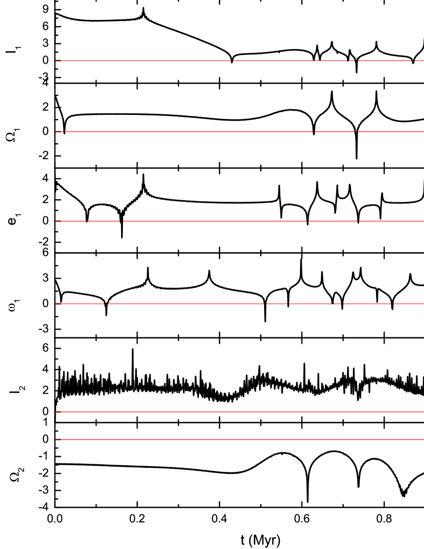
Figure 5: The evolution of $\log[(dx/dt)_{p}/(dx/dt)_{\rm disk}]$ ($x$ represents $I_{1}$, $\Omega_{1}$, $e_{1}$, $\omega_{1}$, $I_{2}$ and $\Omega_{2}$) with time for the case in Figure 1. Red line is the boundary where $(dx/dt)_{p}=(dx/dt)_{\rm disk}$.

In order to obtain the timescales more explicitly, we first assume the initial eccentricities and inclinations of both planets are small before they are effectively excited. We further assume that $m_{2}\geq m_{1}$, and $a_{2}\gg a_{1}$, so the evolution of $m_{2}$ is dominated by perturbations from the disk, and that of $m_{1}$ is mainly affected by perturbations from $m_{2}$ (also see Figure 5).

Under these assumptions, we use Lagrange equations (Murray & Dermott, 1999) to derive the apsidal and nodal precession rate exerted by the disk gravity (see Appendix B for details)

$$\dot{\Omega}_{i,\rm disk}=\frac{3}{2n_{i}}K\cos{I_{i}},$$ (3)

$$\dot{\omega}_{i,\rm disk}=-\frac{2}{n_{i}}K,$$ (4)

where $I_{i}$ and $\Omega_{i}$ are the inclinations and ascending nodes of the two planets ($i=1,2$) with respect to the disk midplane, $\omega_{i}$ is the argument of perihelion, $n_{i}$ is the angular velocity of planetary mean motion, and

$$K=\frac{-\alpha+2}{1-\eta^{-\alpha+2}}\frac{-1+\eta^{-1-\alpha}}{-1-\alpha}\frac{GM_{\rm disk}}{2R_{\rm out}^{3}}$$ (5)

is merely related to the disk parameters, $\eta=R_{\rm in}/R_{\rm out}$, $\alpha$ is the exponential index of disk profile.

In deriving Equations (3)-(4), terms with $e^{2}$ and $\sin^{2}{I}$ have been eliminated to simplify the expressions, which is suitable before the exciting of $e$ and $I$. Meanwhile, under these assumptions, the semi-major axis $a$, eccentricity $e$ and inclination $I$ of each planet have no secular trend from disk gravity (see Appendix B). So the timescales of planet apsidal and nodal precession from disk gravity can be estimated by $2\pi/\dot{\omega}$ and $2\pi/\dot{\Omega}$ separately. Then the timescales of the outer planet are

$$\tau_{\Omega_{2}}=\frac{2\pi}{\dot{\Omega}_{2,\rm disk}},\qquad\qquad\tau_{\omega_{2}}=\frac{2\pi}{\dot{\omega}_{2,\rm disk}}.$$ (6)

Moreover, we apply the secular perturbation theory (Murray & Dermott, 1999) to obtain the precession timescale of the inner planet due to planetary interactions. There are two eigenfrequencies $g_{1}$, $g_{2}$ (where $g_{1}>g_{2}$) for $e-\omega$ solution and one eigenfrequency $f$ for $I-\Omega$ solution in two-planet systems. So

$$\tau_{\Omega_{1}}=\frac{2\pi}{f},\qquad\qquad\tau_{\omega_{1}}=\frac{2\pi}{g_{1}}$$ (7)

can be used to display the precession of $\Omega_{1}$ and $\omega_{1}$ respectively.

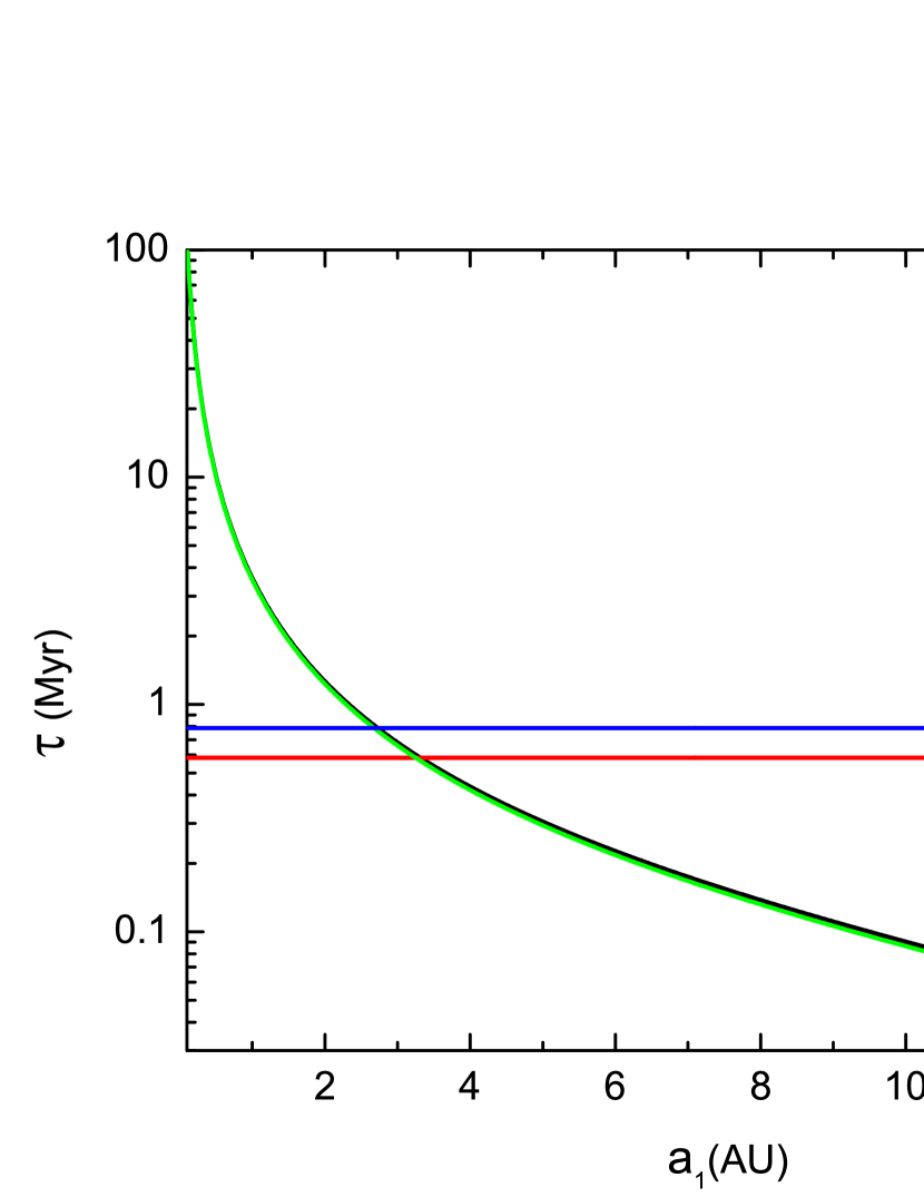
Figure 4: Precession timescales of argument of pericenter $\omega$ and longitude of ascending node $\Omega$ of two planets. Initial parameter is listed in Table 1, except for $I_{2,0}=0$, and $a_{1}$ altering from 0 to 15au. Secular resonance for $e-\omega$ would take place around 3.3au, the place $\tau_{\omega_{1}}=\tau_{\omega_{2}}$, and secular resonance for $I-\Omega$ around 2.7au, the place $\tau_{\Omega_{1}}=\tau_{\Omega_{2}}$.

Figure 4 shows these timescales versus the inner planet’s semi-major axis, with initial condition the same as Figure 3 except $I_{2,0}=0$. $\tau_{\Omega_{1}}$ and $\tau_{\Omega_{2}}$, $\tau_{\omega_{1}}$ and $\tau_{\omega_{2}}$ respectively have one cross point in Figure 4. The x-coordinations of the points display the value of $a_{1,0}$ when VSR and ESR occur, which roughly match the location of pumping at $I_{2,0}=0$ in Figure 3. And the y-coordinations estimate the timescales of secular resonances, which are much less than the average ages of gas disk (Haishch et al., 2001).

When $I_{2,0}>0$, $\tau_{\Omega_{2}}$ becomes larger(Equation (3)), then the cross point of $\tau_{\Omega_{1}}$ and $\tau_{\Omega_{2}}$ would move inward along the $\tau_{\Omega_{1}}$ line. So it only provides the estimation of the inner border of the excitation region in Figure 3. In order to estimate the excitation region more precisely, we will give the evolution equations of the elements in the next section.

4 Evolution equations at arbitrary inclinations

To obtain the quantitative description of planetary orbits when secular resonance happens, we will develop a set of simplified equations to describe the evolutions of $e_{1}$,$\omega_{1}$,$I_{1},\Omega_{1}$, $I_{2},\Omega_{2}$, which are suitable for arbitrary inclinations (but still require for small $e_{2}$). We set the disk midplane as the reference plane, which is assumed to coincide with the equatorial plane of the center star. So our derivations are different with Naoz et al. (2011b) in the context of three-body systems, as their reference plane is the invariable plane of the system.

At first, according to Mardling & Lin (2002), the secular evolution of the elements of $m_{1}$ effected by $m_{2}$ is expressed into the angular momentum vector $\textit{{h}}=\textit{{r}}\bf{\times}\dot{\textit{{r}}}$, the Runge-Lenz vector e and $\hat{\textit{{q}}}=\hat{\textit{{h}}}\bf{\times}\hat{\textit{{e}}}$ (see Equation (A3)-(A6))(The hat indicates the unit vector). And for $m_{2}$, the correspond vectors are $\textit{{H}},\textit{{E}}$ and Q. Then time-averaging is executed, first over the inner orbit for eliminating eccentric anomaly $E_{1}$ then over the outer orbit for removing $E_{2}$ (the results see Equation (A9)-(A14)). Then after, we expand the two groups of unit vectors $(\hat{\textit{{e}}},\hat{\textit{{q}}},\hat{\textit{{h}}})$ and $(\hat{\textit{{E}}},\hat{\textit{{Q}}},\hat{\textit{{H}}})$ into terms with $I_{1}$, $\omega_{1}$, $\Omega_{1}$ and $I_{2}$, $\omega_{2}$, $\Omega_{2}$ separately(see Equation (A)). This is the key step to make the final formulas relative to an arbitrary plane rather than the invariable plane of two orbits. Finally, we obtain the evolutions of the elements due to planetary perturbation up to the quadrupole terms, without any reductions on the eccentricities and inclinations (see Equation (A16)-(A21)). It is worth mentioning that, the evolutions of $e_{1}$ and $\omega_{1}$ has no assumption of $\Delta\Omega=\pi$, so has more terms than the quadrupole parts in formula (C9) and (C5) of Naoz et al. (2011b).

The disturbing from gas disk is been considered independently. Details are in Appendix B. The final evolutions can be acquired by adding the two parts together,

$$\frac{dx}{dt}=(\frac{dx}{dt})_{p}+(\frac{dx}{dt})_{\rm disk}.$$ (8)

$x$ represents the six elements $I_{1}$,$I_{2}$,$\Omega_{1}$,$\Omega_{2}$,$e_{1}$ and $\omega_{1}$. We set $e_{2}=0$ as $e_{2}$ keeps small in most cases (Fig. 3d), then the six equations presented by the above one become closed (we call them “the evolution equations” hereafter).

We made comparisons for the two parts of the evolution equations by drawing $\log[(dx/dt)_{p}/(dx/dt)_{\rm disk}]$ from true N-body simulation in Figure 5. As was expected, for the elements of $m_{1}$, $(dx/dt)_{p}\gg(dx/dt)_{\rm disk}$ in most time, and for $\Omega_{2}$, $(d\Omega_{2}/dt)_{p}\ll(d\Omega_{2}/dt)_{\rm disk}$ all the time. As for $I_{2}$, the influence from disk is much smaller because of the small $e_{2}$ (see Equation (B8)). These can be utilized in the further deductions and simplifications.

Via the evolution equations, we can calculate the evolution of inclination and eccentricity of the inner planet more quickly. The dashed line in Figure 1 displays the integration results from the evolution equations. Except for some delay, both the trend and the amplitude are fitted pretty well. And further, we use the evolution equations to make scanning over $a_{1,0}-I_{2,0}$ (the black contour lines in Figure 3a-c, which is made up of the maximums of the evolutions of 1Myr or before $e_{1}>0.99$ for every case) to compare with the full N-body results. The simplified results agree well qualitatively with the full N-body ones, except some malposition, which mostly results from the quadrupole approximation for disk gravity.

5 Parameter analysis

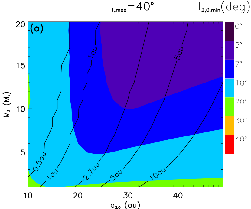
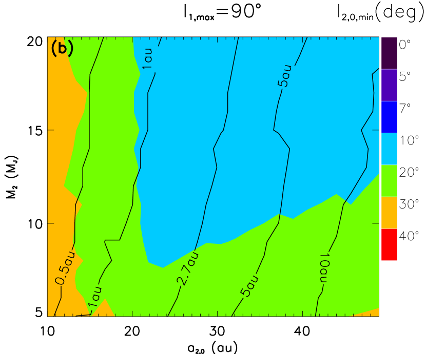
Figure 6: With different $a_{2,0}$ and $m_{2}$, the left panel displays the minimum of initial inclination of the outer planet (filled color contour) for cases in which $I_{\rm tot}$ could reach $40^{\circ}$ during evolution ($y$ coordinations of the star in Figure 3a). The solid line contour is made up of locations of the inner planet when $I_{\rm tot,max}=40^{\circ}$ happens with the smallest $I_{2,0}$ ($x$ coordinations of the star in Figure 3a). The right panel has similar meanings except for $I_{1}$ reaching $90^{\circ}$ during evolution (the coordination of the star in Figure 3b). Every $a_{1,0}-I_{2,0}$ scanning involved is from the same condition as the black line contours in Figure 3.

According to Figure 3, Kozai resonance between planets occurred above the contour line of $I_{\rm tot,max}=40^{\circ}$, and the retrograde motion of $m_{1}$ happened above the line of $I_{\rm 1,max}=90^{\circ}$. As planets were thought to be coplanar at their earliest stage, lower values of extremum of these two contour lines would make the generation of retrograde motion easier. For this purpose, we investigate the dependence of the minimums of $I_{\rm 1,max}=90^{\circ}$ and $I_{\rm tot,max}=40^{\circ}$ on $a_{2,0}$ and $m_{2}$ with the evolution equation (8)(Fig. 6), with the parameters the same as Figure 4 except for the variables $a_{2,0}$, $m_{2}$ and the scanned $I_{2,0}$, $a_{1,0}$. Filled color contour is composed of the values of y-coordinate of the extremum ($I_{2,0,\rm min}$), which means the smallest inclination of $m_{2}$ for the onset of Kozai effect ($I_{\rm tot,max}=40^{\circ}$) or for $m_{1}$ retrograding ($I_{\rm 1,max}=90^{\circ}$). The solid line contour is built up by x-coordinates of the extremum, which signify the locations of $m_{1}$ when VSR between planets will occur.

Considering a Jupiter-mass planet most probably formed outside the snowline (2.7au for a $1M_{\odot}$ star, see Ida & Lin 2004), we constrain the interesting scope beyond 2.7au for solid contour in Figure 6. We can see that with a $0.05M_{\odot}$ gas disk ranging from 50au to 1000au, a Jupiter-mass planet at $\sim 2.7$au will be pumped by Kozai effect with a $5m_{J}$ planet at 25au and inclined $>10^{\circ}$ relative to the disk midplane. Further more, it can be flipped into a retrograde orbit by a giant planet at $\sim 25$ au with mass of $5m_{J}$ and inclination $>30^{\circ}$, or mass of $10m_{J}$ with inclination $>20^{\circ}$. As every $a_{1,0}-I_{2,0}$ scanning involved in Figure 6 is made up of the $\leq 1$ Myr integrations of the evolution equations, a general gas disk aged several million years is enough for the excitation process.

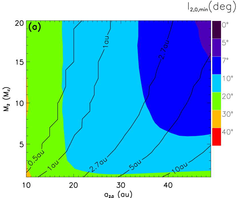
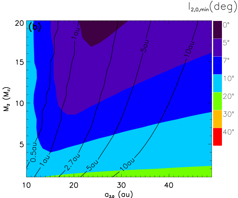
Figure 7: The same as Figure 6a, except for (a) $M_{disk}=20M_{J}$. (b) $M_{disk}=100M_{J}$.

We also investigate the affection of disk mass on the exciting process. Figure 7 gives the scanning results like figure 6a for $M_{\rm disk}=20M_{J}$ and $M_{\rm disk}=100M_{J}$. Other parameters keep the same as in table 1 for simplicity. For the smaller disk mass (Fig.7a), the regions of $I_{2,0,\rm min}$ move toward upper and right relative to the same ones in figure 6a, which causes the zone of lower $I_{2,0,\rm min}$ smaller. And for the bigger disk mass (Fig.7b), the $I_{2,0,\rm min}=5^{\circ}\sim 7^{\circ}$ range extends to the less massive $M_{2}$-region as compared to figure 6a, and the $I_{2,0,\rm min}=0^{\circ}\sim 5^{\circ}$ range appears in the upper. So a more massive disk is in favor of the pumping to some extent.

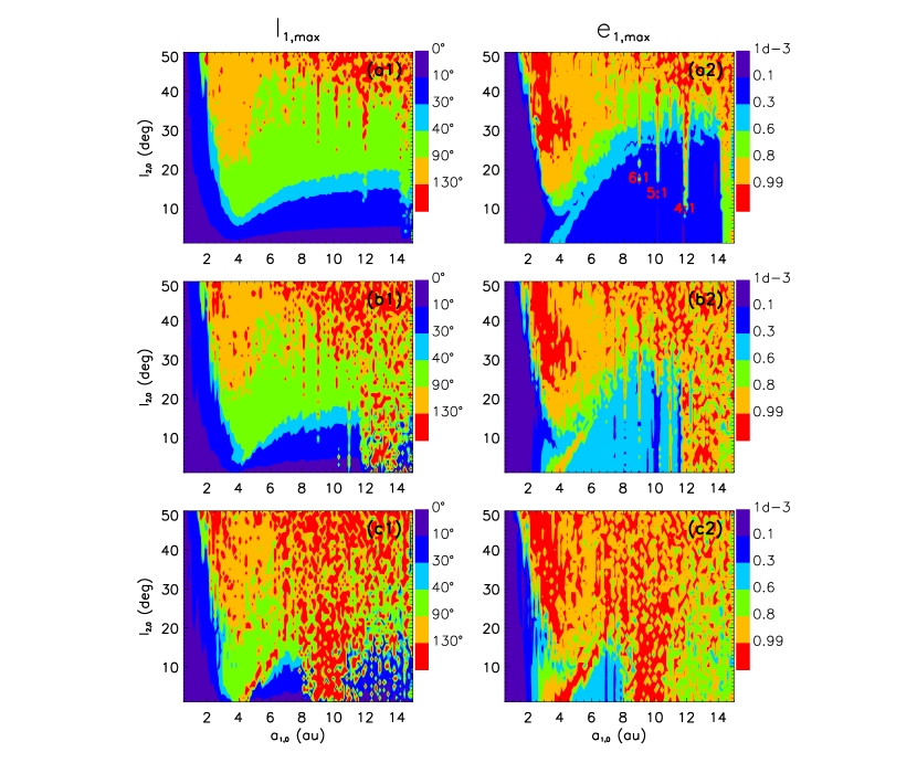
Figure 8: The same as the results of N-body simulation in Figure 3a (the left ones) and 3c (the right ones), except for (a) $e_{2,0}=0.2$. (b) $e_{2,0}=0.35$. (c) $e_{2,0}=0.5$. The red numbers in the panel (a2) mean the period ratios of two planets.

All the above discussions have set $e_{2,0}=0.001$ for concentrating on VSR more conveniently. However, $m_{2}$ is more likely on an eccentric orbit since the planetary scattering have prompted a non-zero inclination. Figure 8 shows the same N-body simulations scanning as those in figure 3b,c with a higher $e_{2,0}$. The remarkable difference in the higher $e_{2,0}$ situation is that the critical value of $I_{2,0}$ for pumping gets smaller. The cases with $I_{1,\rm max}>90^{\circ}$ and $e_{1,\rm max}>0.99$ appear even when $I_{2,0}=0^{\circ}$, which might be due to the strong couplings between ESR and VSR when $e_{2}$ is large. However, the effect is not obvious when $e_{2,0}<0.2$.

In Fig.8, we also notice that at small $e_{2,0}$ (Fig.8a), planetary mean motion resonances (4:1, 5:1,6:1) cause an increase of $I_{1,\rm max}$ and $e_{1,\rm max}$. When $e_{2,0}$ becomes larger, the regions outside 12AU in Fig.8b and 8AU in Fig.8c are full of the cases with $I_{1,\rm max}>130^{\circ}$ and $e_{1,\rm max}>0.99$, this is due to that, as the apohelion of the inner planet is comparable to the perihelion of the outer planet, then planetary scattering dominates. We stop the simulation as long as any planet crosses the inner edge of the disk.

6 Systems with more than two planets

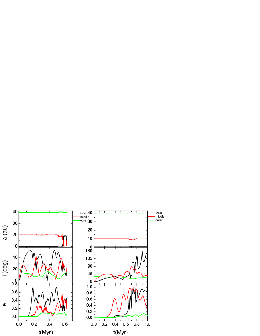
Figure 9: Two cases of evolution of semi-major axis, inclinations and eccentricities of three planets, which orbit the center star with a disk outside. The left plot has three planets with $m_{1}=1m_{J},m_{2}=1m_{J},m_{3}=5m_{J},a_{1}=10{\rm au},a_{2}=20{\rm au},a_{3}=40{\rm au},I_{1}=1^{\circ},I_{2}=1^{\circ},I_{3}=20^{\circ}$, and three planets in the right plot are $m_{1}=0.1m_{J},m_{2}=1m_{J},m_{3}=5m_{J},a_{1}=1{\rm au},a_{2}=10{\rm au},a_{3}=40{\rm au},I_{1}=1^{\circ},I_{2}=1^{\circ},I_{3}=30^{\circ}$, The disk parameters are the same as Table 1.

With the help of the VSR, a mutual inclination between planetary orbits much smaller than the Kozai critical value can induce the pumping of the inner planet’s eccentricity eventually. However, the occurrence of VSR constrains the inner orbit to a narrow trigger range, and the opportunity is small that two adjacent planets happen to be in the VSR configuration. Actually, the above pumping mechanism can be extended to multiple planetary systems so that a wider trigger range can be achieved. Here we give two examples to show that the mechanism can also occur between two nonadjacent planets, as well as inspire a chain reaction among more than two planets. In the left case of Figure 9, the innermost and outermost planets were right in a configuration to be excited in a two-planet situation, and after another planet is added between them, the excitation still turns up. The right case in Figure 9 exhibits a chain reaction. The middle planet is located right in the VSR scope of the outermost planet, so its inclination is pumped at first, which directly leads to the increase of the mutual inclination of the inner two planets. At last, the innermost planet is excited by the VSR with the middle planet. So the influence of excitation of the outer planet can be spread to a more inward scope by a chain reaction. We do not explore the specific conditions or detailed influence of these more complicated operations of the mechanism, and leave them to future works.

7 Conclusions and discussions

In this paper, we proposed a mechanism to excite the eccentricities and inclinations of planets with a residual gas disk outside the planets. The excitation was the results of a coupling of secular resonance and Kozai effect. After several giant planets formed, the inner disk was assumed to have been swept out by gas giants during their accretion, and the outer part of gas disk would coexist with planets as long as million years. If the outermost planet has a moderately inclined orbit relative to the disk midplane, vertical secular resonance would happen between the planets. Then the mutual inclination between two planets increases. Once it reaches up to $\sim 40^{\circ}$, the Kozai effect between the planets would be induced, which can further pump the inner planet’s eccentricity and inclination to high values (Fig. 1). So this kind of mechanism is probably one of origins of hot-Jupiters on misaligned even retrograde orbits.

To describe the evolution of inclinations and longitude of ascending nodes, we derived the evolution Equations, which are closed with the assumption of $e_{2}=0$, and are suitable for arbitrary inclinations. They are used to find out the locations and minimum initial inclinations for the occurrence of vertical secular resonance and Kozai resonance (Fig. 3, 6). The elements here are relative to the disk midplane, and the formulas are different with those of the elements relative to the invariable plane of the two orbits. So they can be utilized to situations with the elements relative to any invariable plane.

From the evolution equations, we showed that, with a mass of $0.05M_{\odot}$ residual gas disk located from 50au to 1000au, a Jupiter-mass planet will be pumped by an outer gas giant with $5m_{J}$ mass and $10^{\circ}$ relative to the disk midplane at least, located out of 25au. And it could be flipped into a retrograde orbit by an outer gas giant with $10m_{J}$ mass and an initial inclination of $20^{\circ}$. Such a mechanism can be also effective for a system with more than two planets, and the critical angles required might be more flexible with the presence of more planets.

We used a simple disk model in order to compare with the results of the evolution equations and fully discuss the effect of planetary parameters. Also the limitation is that the disk mass have to be much bigger than the total mass of planets for satisfying the angular-momentum-advantage assumption(section 2), which restricts the full discussion to the disc parameters. To verify that the pumping process is irrelative to disk model, we made the same simulations using a different disk model (Nagasawa et al., 2000; Zhao et al., 2011). Then we found the pumping still exists with similar structures and even locations of contour lines in Figure 3.

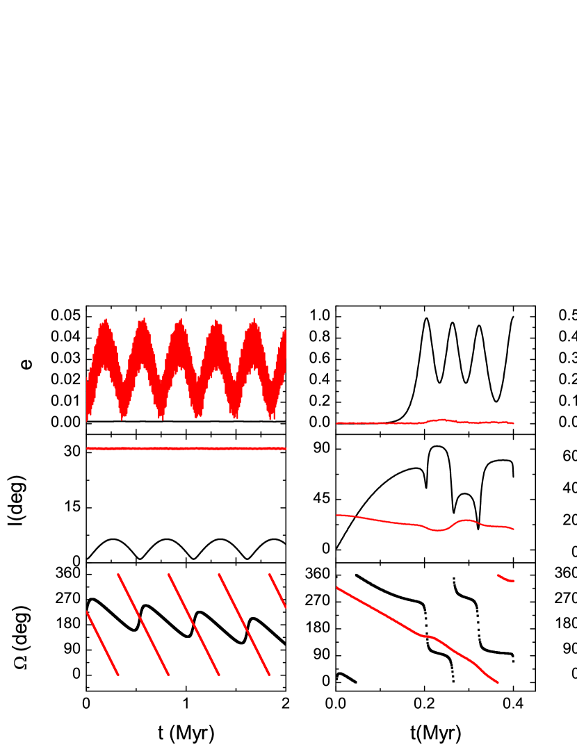
Figure 10: These are three cases representing three different kinds of evolution of the inner planet. The only different initial condition is the semi-major axis of the inner planet $a_{1,0}$, which is 0.56au, 4.33au and 9.4au from left to right. Other parameters are the same, $m_{1}=1m_{J},m_{2}=5m_{J},m_{\rm disk}=50m_{J},a_{2}=20{\rm au},R_{\rm in}=30{\rm au},R_{\rm out}=1000{\rm au},I_{1}=1^{\circ},I_{2}=31^{\circ},e_{1}=e_{2}=0.001,\Omega_{1}=\Omega_{2}$. All arguments are arbitrary. Black lines are for the elements of the inner planet and red lines for these of the outer planet.

The mechanism revealed above has some resemblance with that in binary systems. In a binary system with two planets orbiting one of the stars, Takeda et al. (2008) divided three distinct dynamical classes according to differential nodal precessions of the two planets. The mechanism illustrated in our paper is similar to the so-called “weakly coupled systems”, with the same peculiarity that the planetary mutual inclination is excited by the secular resonance between the planets. That is actually a transitional case between “decoupled systems” and “dynamically rigid systems”. We illustrate this from the three cases in Figure 10, where the semi-axis of the inner planet is the only varying parameter. In the left case, the planetary secular interaction is very weak and suppressed by the perturbation from the disk, so the secular nodal precession of the inner planet is much slower than that of the outer planet. In the right case, the mutual effects between the planets become so strong that their nodal precesses coupled, and the maximum of their mutual inclination is roughly the sum of $I_{1,0}$ and $I_{2,0}$. The middle case is an exciting one, which occurs when planetary interaction is big enough that the secular nodal precessions of the two planets are approaching but not too big that the planets are coupled.

In this respect, a protoplanetary disk has a comparable effect with a stellar companion. Actually, this kind of analogy has been mentioned in Wu & Lithwick (2011). They pointed out that the place of a planet in secular interactions could be replaced by a mass wire made by spreading the planet along its orbit. Since protoplanetary disks are universal in single-star systems, our exciting mechanism induced by secular resonance would not be limited in binary systems but can be extended to single-star systems.

Though in our mechanism, eccentricity pumping can occur with an initial mutual inclination much smaller than the Kozai critical angle, it is still within a rather narrow range of disk and planet configurations for a Jupiter-mass planet can be flipped. The efficiency for the occurrence of this mechanism in different systems will be investigated in future works. Comparing to observations, the narrow range also implies that, firstly, there should be most of systems owing planets with moderate or low eccentricities and inclinations than the systems owing retrograde hot-Jupiters. Secondly, according to our additional simulations, the more massive the inner planet is, the higher the initial outer inclination is demanded to be, meanwhile, the more massive the outer planet needs to be. So we speculate that the proportion of misalignment in Earth-like or Neptune-like planets is probably larger than that in Jupiter-like planet. All these need to be verified by further statistics of simulations as well as observations.

Appendix A Evolution of the orbital elements due to planetary perturbation

We apply Legendre polynomials expansion and Runge-Lenz vector introduced in Mardling & Lin (2002) to deduce the elements’ evolution due to planetary interactions. The quadrupole contribution of the acceleration of the inner orbit produced by the third body is

$$\textit{{f}}_{1,p}=\frac{Gm_{2}}{R^{3}}(3x\hat{\textit{{R}}}-\textit{{r}}),$$ (A1)

and that of the outer planet from the inner one is

$$\textit{{f}}_{2,p}=-\frac{G\mu_{01}}{R^{4}}\frac{m_{012}}{m_{01}}\Bigg{[}\frac{3}{2}(5x^{2}-r^{2})\hat{\textit{{R}}}-3x\textit{{r}}\Bigg{]},$$ (A2)

where r and R are position vectors of the inner and outer planet in Jacobi coordinates, $x=\textit{{r}}\cdot\hat{\textit{{R}}}$, $m_{012}=m_{0}+m_{1}+m_{2}$, $m_{01}=m_{0}+m_{1}$, $\mu_{01}=m_{0}m_{1}/m_{01}$.

The relations between the rates of change of the inner orbital elements and those of Runge-Lenz vectors are given by

$$\frac{de_{1}}{dt}=\dot{\textit{{e}}}\cdot\hat{\textit{{e}}},$$ (A3)

$$\frac{d\omega_{1}}{dt}=-\frac{d\Omega_{1}}{dt}\cos{I_{1}}+\frac{\dot{\textit{{e}}}}{e_{1}}\cdot\hat{\textit{{q}}},$$ (A4)

$$\frac{dI_{1}}{dt}=\frac{-(\sin{\omega_{1}}\hat{\textit{{e}}}+\cos{\omega_{1}}\hat{\textit{{q}}})\cdot\dot{\textit{{h}}}}{h_{1}},$$ (A5)

$$\frac{d\Omega_{1}}{dt}=\frac{(\cos{\omega_{1}}\hat{\textit{{e}}}-\sin{\omega_{1}}\hat{\textit{{q}}})\cdot\dot{\textit{{h}}}}{h_{1}\sin{I_{1}}},$$ (A6)

where

$$\frac{d\textit{{e}}}{dt}=\frac{2(\textit{{f}}\cdot\dot{\textit{{r}}})\textit{{r}}-(\textit{{r}}\cdot\dot{\textit{{r}}})\textit{{f}}-(\textit{{f}}\cdot\textit{{r}})\dot{\textit{{r}}}}{Gm_{01}},$$ (A7)

$$\frac{d\textit{{h}}}{dt}=\textit{{r}}\times\textit{{f}}.$$ (A8)

$\textit{{h}}=\textit{{r}}\bf{\times}\dot{\textit{{r}}}$ is the orbital angular momentum vector of the inner orbit, $\hat{\textit{{e}}}$ is the Runge-Lenz vector and $\hat{\textit{{q}}}=\hat{\textit{{h}}}\bf{\times}\hat{\textit{{e}}}$. $\textit{{r}}=a_{1}(\cos{E_{1}}-e_{1})\hat{\textit{{e}}}+a_{1}\sqrt{1-e_{1}^{2}}\sin{E_{1}}\hat{\textit{{q}}}$, $\dot{\textit{{r}}}=-a_{1}n_{1}\sin{E_{1}}/(1-e_{1}\cos{E_{1}})\hat{\textit{{e}}}+a_{1}n_{1}\sqrt{1-e_{1}^{2}}\cos{E_{1}}/(1-e_{1}\cos{E_{1}})\hat{\textit{{q}}}$. For the outer orbit, r would be replaced by R, and the correspond unit vector is $(\hat{\textit{{E}}},\hat{\textit{{Q}}},\hat{\textit{{H}}})$.

We separately substitute the expressions (A1) and (A2) for f in (A3)-(A6), and average first over the inner orbit then the outer orbit, and simplify the results as follow

$$(\frac{di_{1}}{dt})_{p} = \frac{3Gm_{2}}{4h_{1}}\frac{a_{1}^{2}}{a_{2}^{3}}(1-e_{2}^{2})^{-3/2}\bigg{[}(\cos{\omega_{1}}\hat{\textit{{e}}}-\sin{\omega_{1}}\hat{\textit{{q}}})+e_{1}^{2}(4\cos{\omega_{1}}\hat{\textit{{e}}}+\sin{\omega_{1}}\hat{\textit{{q}}})\bigg{]}$$ (A9)

$$\cdot\bigg{[}(\hat{\textit{{h}}}\cdot\hat{\textit{{E}}})\hat{\textit{{E}}}+(\hat{\textit{{h}}}\cdot\hat{\textit{{Q}}})\hat{\textit{{Q}}}\bigg{]},$$

$$(\frac{d\Omega_{1}}{dt})_{p} = \frac{3Gm_{2}}{4h_{1}\sin{i_{1}}}\frac{a_{1}^{2}}{a_{2}^{3}}(1-e_{2}^{2})^{-3/2}\bigg{[}(\sin{\omega_{1}}\hat{\textit{{e}}}+\cos{\omega_{1}}\hat{\textit{{q}}})+e_{1}^{2}(4\sin{\omega_{1}}\hat{\textit{{e}}}-\cos{\omega_{1}}\hat{\textit{{q}}})\bigg{]}$$ (A10)

$$\cdot\bigg{[}(\hat{\textit{{h}}}\cdot\hat{\textit{{E}}})\hat{\textit{{E}}}+(\hat{\textit{{h}}}\cdot\hat{\textit{{Q}}})\hat{\textit{{Q}}}\bigg{]},$$

$$(\frac{di_{2}}{dt})_{p} = \frac{3G\mu_{01}m_{012}}{4h_{2}m_{01}}\frac{a_{1}^{2}}{a_{2}^{3}}(1-e_{2}^{2})^{-3/2}(\cos{\omega_{2}}\hat{\textit{{E}}}-\sin{\omega_{2}}\hat{\textit{{Q}}})\cdot\bigg{[}(1+4e^{2}_{1})(\hat{\textit{{H}}}\cdot\hat{\textit{{e}}})\hat{\textit{{e}}}$$ (A11)

$$+(1-e^{2}_{1})(\hat{\textit{{H}}}\cdot\hat{\textit{{q}}})\hat{\textit{{q}}}\bigg{]},$$

$$(\frac{d\Omega_{2}}{dt})_{p} = \frac{3G\mu_{01}m_{012}}{4h_{2}m_{01}\sin{i_{1}}}\frac{a_{1}^{2}}{a_{2}^{3}}(1-e_{2}^{2})^{-3/2}(\sin{\omega_{2}}\hat{\textit{{E}}}+\cos{\omega_{2}}\hat{\textit{{Q}}})\cdot\bigg{[}(1+4e^{2}_{1})(\hat{\textit{{H}}}\cdot\hat{\textit{{e}}})\hat{\textit{{e}}}$$ (A12)

$$+(1-e^{2}_{1})(\hat{\textit{{H}}}\cdot\hat{\textit{{q}}})\hat{\textit{{q}}}\bigg{]},$$

$$(\frac{de_{1}}{dt})_{p} = -\frac{15m_{2}a_{1}^{3}}{4m_{01}a_{2}^{3}}n_{1}e_{1}\sqrt{1-e_{1}^{2}}(1-e_{2}^{2})^{-3/2}\bigg{[}(\hat{\textit{{e}}}\cdot\hat{\textit{{E}}})(\hat{\textit{{q}}}\cdot\hat{\textit{{E}}})+(\hat{\textit{{e}}}\cdot\hat{\textit{{Q}}})(\hat{\textit{{q}}}\cdot\hat{\textit{{Q}}})\bigg{]},$$ (A13)

$$(\frac{d\omega_{1}}{dt})_{p} = -(\frac{d\Omega_{2}}{dt})_{p}\cos{I_{1}}+\frac{3m_{2}a_{1}^{3}}{4m_{01}a_{2}^{3}}n_{1}\sqrt{1-e_{1}^{2}}(1-e_{2}^{2})^{-3/2}\Big{\{}4\big{[}(\hat{\textit{{e}}}\cdot\hat{\textit{{E}}})^{2}+(\hat{\textit{{e}}}\cdot\hat{\textit{{Q}}})^{2}\big{]}$$ (A14)

$$-\big{[}(\hat{\textit{{q}}}\cdot\hat{\textit{{E}}})^{2}+(\hat{\textit{{q}}}\cdot\hat{\textit{{Q}}})^{2}\big{]}-2\Big{\}}.$$

The coordinates of the Runge-Lenz vectors relative to an arbitrary inertial plane are

$$\hat{\textit{{e}}}=\left(\begin{array}[]{c}\cos{\Omega_{1}}\cos{\omega_{1}}-\sin{\Omega_{1}}\sin{\omega_{1}}\cos{i_{1}}\\ \sin{\Omega_{1}}\cos{\omega_{1}}+\cos{\Omega_{1}}\sin{\omega_{1}}\cos{i_{1}}\\ \sin{i_{1}}\sin{\omega_{1}}\end{array}\right),$$

$$\hat{\textit{{q}}}=\left(\begin{array}[]{c}-\cos{\Omega_{1}}\sin{\omega_{1}}-\sin{\Omega_{1}}\cos{\omega_{1}}\cos{i_{1}}\\ -\sin{\Omega_{1}}\sin{\omega_{1}}+\cos{\Omega_{1}}\cos{\omega_{1}}\cos{i_{1}}\\ \sin{i_{1}}\cos{\omega_{1}}\end{array}\right),$$

$$\hat{\textit{{h}}}=\left(\begin{array}[]{c}\sin{i_{1}}\sin{\Omega_{1}}\\ -\sin{i_{1}}\cos{\Omega_{1}}\\ \cos{i_{1}}\end{array}\right),$$ (A15)

and for $\hat{\textit{{E}}},\hat{\textit{{Q}}},\hat{\textit{{H}}}$, the formulas are similar except for switching the subscripts from 1 to 2.

Then we derived the final simplified expressions for the rates of change of $I_{1}$,$I_{2}$,$\Omega_{1}$,$\Omega_{2}$,$e_{1}$ and $\omega_{1}$

$$(\frac{dI_{1}}{dt})_{p} = \frac{3m_{2}a_{1}^{3}n_{1}}{4m_{01}a_{2}^{3}}(1-e_{1}^{2})^{-1/2}(1-e_{2}^{2})^{-3/2}\bigg{[}\cos{I_{1}}\cos{I_{2}}+\sin{I_{1}}\sin{I_{2}}\cos(\Omega_{1}-\Omega_{2})\bigg{]}$$ (A16)

$$\times\Bigg{\{}\sin{I_{2}}\sin(\Omega_{1}-\Omega_{2})+\frac{1}{2}e_{1}^{2}\bigg{[}(3+5\cos{2\omega_{1}})\sin{I_{2}}\sin(\Omega_{1}-\Omega_{2})$$

$$+5\sin{2\omega_{1}}(\cos{I_{1}}\sin{I_{2}}\cos(\Omega_{1}-\Omega_{2})-\sin{I_{1}}\cos{I_{2}})\bigg{]}\Bigg{\}},$$

$$(\frac{dI_{2}}{dt})_{p} = \frac{3m_{0}m_{1}a_{1}^{2}n_{2}}{4m_{01}^{2}a_{2}^{2}}(1-e_{2}^{2})^{-2}\Bigg{\{}-\sin{I_{1}}\sin(\Omega_{1}-\Omega_{2})\bigg{[}\cos{I_{1}}\cos{I_{2}}$$ (A17)

$$+\sin{I_{1}}\sin{I_{2}}\cos(\Omega_{1}-\Omega_{2})\bigg{]}+\frac{1}{2}e_{1}^{2}\bigg{[}-3\sin{I_{1}}\sin(\Omega_{1}-\Omega_{2})\big{(}\cos{I_{1}}\cos{I_{2}}$$

$$+\sin{I_{1}}\sin{I_{2}}\cos(\Omega_{1}-\Omega_{2})\big{)}+5\cos{2\omega_{1}}\sin(\Omega_{1}-\Omega_{2})\big{(}\sin{I_{1}}\cos{I_{1}}\cos{I_{2}}$$

$$-(1+\cos^{2}{I_{1}})\sin{I_{2}}\cos(\Omega_{1}-\Omega_{2})\big{)}+5\sin{2\omega_{1}}\big{(}\sin{I_{1}}\cos{I_{2}}\cos(\Omega_{1}-\Omega_{2})$$

$$-\cos{I_{1}}\sin{I_{2}}\cos{2(\Omega_{1}-\Omega_{2})}\big{)}\bigg{]}\Bigg{\}},$$

$$(\frac{d\Omega_{1}}{dt})_{p} = \frac{3m_{2}a_{1}^{3}n_{1}}{4m_{01}a_{2}^{3}\sin{I_{1}}}(1-e_{1}^{2})^{-1/2}(1-e_{2}^{2})^{-3/2}\Bigg{\{}\frac{1}{4}\sin{I_{1}}\cos{I_{1}}\bigg{[}2\cos{2(\Omega_{1}-\Omega_{2})}\sin^{2}{I_{2}}$$ (A18)

$$-3\cos{2I_{2}}-1\bigg{]}+\frac{1}{2}\cos{2I_{1}}\sin{2I_{2}}\cos(\Omega_{1}-\Omega_{2})+\frac{1}{2}e_{1}^{2}\bigg{[}\cos{I_{1}}\cos{I_{2}}$$

$$+\sin{I_{1}}\sin{I_{2}}\cos(\Omega_{1}-\Omega_{2})\bigg{]}\bigg{[}(-3+5\cos{2\omega_{1}})\big{(}\sin{I_{1}}\cos{I_{2}}$$

$$-\cos{I_{1}}\sin{I_{2}}\cos(\Omega_{1}-\Omega_{2})\big{)}+5\sin{I_{2}}\sin{2\omega_{1}}\sin(\Omega_{1}-\Omega_{2})\bigg{]}\Bigg{\}},$$

$$(\frac{d\Omega_{2}}{dt})_{p} = \frac{3m_{0}m_{1}a_{1}^{2}n_{2}}{4m_{01}^{2}a_{2}^{2}\sin{I_{2}}}(1-e_{2}^{2})^{-2}\Bigg{\{}\frac{1}{4}\sin{I_{2}}\cos{I_{2}}\bigg{[}2\cos{2(\Omega_{1}-\Omega_{2})}\sin^{2}{I_{1}}-3\cos{2I_{1}}-1\bigg{]}$$ (A19)

$$+\frac{1}{2}\sin{2I_{1}}\cos{2I_{2}}\cos(\Omega_{1}-\Omega_{2})+\frac{1}{4}e_{1}^{2}\bigg{[}3\sin{2I_{2}}\big{(}-\cos^{2}{I_{1}}+\sin^{2}{I_{1}}\cos^{2}(\Omega_{1}-\Omega_{2})\big{)}$$

$$+3\sin{2I_{1}}\cos{2I_{2}}\cos(\Omega_{1}-\Omega_{2})-5\cos{2\omega_{1}}\sin{2I_{1}}\cos{2I_{2}}\cos(\Omega_{1}-\Omega_{2})$$

$$+5\cos{2\omega_{1}}\sin{2I_{2}}\big{(}\cos^{2}{I_{1}}\cos^{2}(\Omega_{1}-\Omega_{2})-\sin^{2}(\Omega_{1}-\Omega_{2})-\sin^{2}{I_{1}}\big{)}$$

$$+10\sin{2\omega_{1}}\sin(\Omega_{1}-\Omega_{2})\big{(}\sin{I_{1}}\cos{2I_{2}}-\cos{I_{1}}\sin{2I_{2}}\cos(\Omega_{1}-\Omega_{2})\big{)}\bigg{]}\Bigg{\}},$$

$$(\frac{de_{1}}{dt})_{p} = \frac{15m_{2}a_{1}^{3}n_{1}}{8m_{01}a_{2}^{3}}e_{1}\sqrt{1-e_{1}^{2}}(1-e_{2}^{2})^{-3/2}\Bigg{\{}\sin{2\omega_{1}}\bigg{[}\big{(}\sin{I_{1}}\cos{I_{2}}-\cos{I_{1}}\sin{I_{2}}\cos(\Omega_{1}-\Omega_{2})\big{)}^{2}$$ (A20)

$$-\sin^{2}{I_{2}}\sin^{2}(\Omega_{1}-\Omega_{2})\bigg{]}-2\cos{2\omega_{1}}\sin{I_{2}}\sin(\Omega_{1}-\Omega_{2})\bigg{[}\sin{I_{1}}\cos{I_{2}}$$

$$-\cos{I_{1}}\sin{I_{2}}\cos(\Omega_{1}-\Omega_{2})\bigg{]}\Bigg{\}},$$

$$(\frac{d\omega_{1}}{dt})_{p} = -(\frac{d\Omega_{1}}{dt})_{p}\cos{I_{1}}-\frac{3m_{2}a_{1}^{3}n_{1}}{4m_{01}a_{2}^{3}}\sqrt{1-e_{1}^{2}}(1-e_{2}^{2})^{-3/2}\Bigg{\{}\big{(}1-5\sin^{2}{\omega_{1}}\big{)}\bigg{[}\big{(}\sin{I_{1}}\sin{I_{2}}$$ (A21)

$$+\cos{I_{1}}\cos{I_{2}}\cos(\Omega_{1}-\Omega_{2})\big{)}^{2}+\sin^{2}(\Omega_{1}-\Omega_{2})\big{(}\cos^{2}{I_{1}}+\sin^{2}{I_{2}}\big{)}-1\bigg{]}$$

$$-5\sin{2\omega_{1}}\sin(\Omega_{1}-\Omega_{2})\sin{I_{2}}\bigg{[}\sin{I_{1}}\cos{I_{2}}-\cos{I_{1}}\sin{I_{2}}\cos(\Omega_{1}-\Omega_{2})\bigg{]}$$

$$+3\sin^{2}{I_{2}}\sin^{2}(\Omega_{1}-\Omega_{2})-1\Bigg{\}}.$$

When $\Omega_{1}-\Omega_{2}=\pi$, the latter two formula turn to the quadrupole parts of (C9) and (C5) of Naoz et al. (2011b).

Appendix B Evolution of the orbital elements due to disk gravity

As in observation, disk mass is a commonly estimated parameter rather than the radial distribution exponential or mass density, we set disk mass as an independent parament and deduce the mass density from

$$\int_{R_{\rm in}}^{R_{\rm out}}\Sigma_{0}\Bigg{(}\frac{r}{R_{\rm out}}\Bigg{)}^{-\alpha}2\pi rdr=M_{\rm disk},$$ (B1)

then obtain

$$\Sigma_{0}=\frac{(-\alpha+2)M_{\rm disk}}{2(1-\eta^{-\alpha+2})\pi R_{\rm out}^{2}}$$ (B2)

with $\eta=R_{\rm in}/R_{\rm out}$.

We used Lagrange’s equations in Murray & Dermott (1999) to deduce the rates of change of elements due to disk gravity. First, we expanded the gravity potential in $r_{p}/r$ to the quadrupole, like Terquem et al. (2010),

$$\Phi=-\frac{-\alpha+2}{1-\eta^{-\alpha+2}}\frac{GM_{\rm disk}}{R_{\rm out}}\Bigg{[}\frac{1-\eta^{1-\alpha}}{1-\alpha}+\frac{-1+\eta^{-1-\alpha}}{1+\alpha}\frac{r_{p}^{2}}{2R_{\rm out}^{2}}\bigg{(}-1+\frac{3}{2}\sin^{2}{\theta_{p}}\bigg{)}\Bigg{]}.$$ (B3)

The first term in the square brackets has no contribution to derivation, so only the second one is retained. Defining

$$K=\frac{-\alpha+2}{1-\eta^{-\alpha+2}}\frac{-1+\eta^{-1-\alpha}}{-1-\alpha}\frac{GM_{\rm disk}}{2R_{\rm out}^{3}},$$ (B4)

then substituted the expresses with true anomaly $f$ for $r_{p}$ and $\theta_{p}$, we got

$$\Phi=K\frac{a^{2}(1-e^{2})^{2}}{(1+e\cos{f})^{2}}\bigg{[}\frac{1}{2}-\frac{3}{2}\sin^{2}{(\omega+f)}\sin^{2}{I}\bigg{]}.$$ (B5)

We substituted the above one into Lagrange’s Equations (6.148)-(6.150) in Murray & Dermott (1999), then averaged over true anomaly $f$, and got the evolutions finally

$$(\frac{da}{dt})_{\rm disk}=0,$$ (B6)

$$(\frac{de}{dt})_{\rm disk}=-\frac{15Ke\beta}{4n}\sin{2\omega}\sin^{2}{I},$$ (B7)

$$(\frac{dI}{dt})_{\rm disk}=\frac{15Ke^{2}}{8n\beta}\sin{2\omega}\sin{2I},$$ (B8)

$$(\frac{d\Omega}{dt})_{\rm disk}=\frac{3K\cos{I}}{4n\beta}(2+3e^{2}-5e^{2}\cos{2\omega}),$$ (B9)

$$(\frac{d\omega}{dt})_{\rm disk}=\frac{K}{n\beta}\Bigg{\{}-2-\frac{9}{8}e^{2}+\frac{15}{4}e^{2}\cos{2\omega}+\sin^{2}{I}\bigg{[}\frac{9}{4}+\frac{9}{16}e^{2}-\frac{15}{16}(2+e^{2})\cos{2\omega}\bigg{]}\Bigg{\}},$$ (B10)

where $\beta=\sqrt{1-e^{2}}$.

When $i\simeq 0$ and $e=0$, the expressions can be simplified into

$$(\frac{da}{dt})_{\rm disk}=(\frac{de}{dt})_{\rm disk}=(\frac{dI}{dt})_{\rm disk}=0$$ (B11)

$$(\frac{d\Omega}{dt})_{\rm disk}=\frac{3K\cos{I}}{2n}$$ (B12)

$$(\frac{d\omega}{dt})_{\rm disk}=-\frac{2K}{n}$$ (B13)

Table 1: Initial condition for Figure 1.

Planet	Mass	Semimajor Axis	Eccentricity	Inclination
	($M_{J}$)	(au)		(∘)
$m_{1}$	1	3	0.001	1
$m_{2}$	10	30	0.001	30
disk	Mass	$R_{\rm in}$	$R_{\rm out}$	$\alpha$
	($M_{J}$)	(au)	(au)
	50	50	1000	1

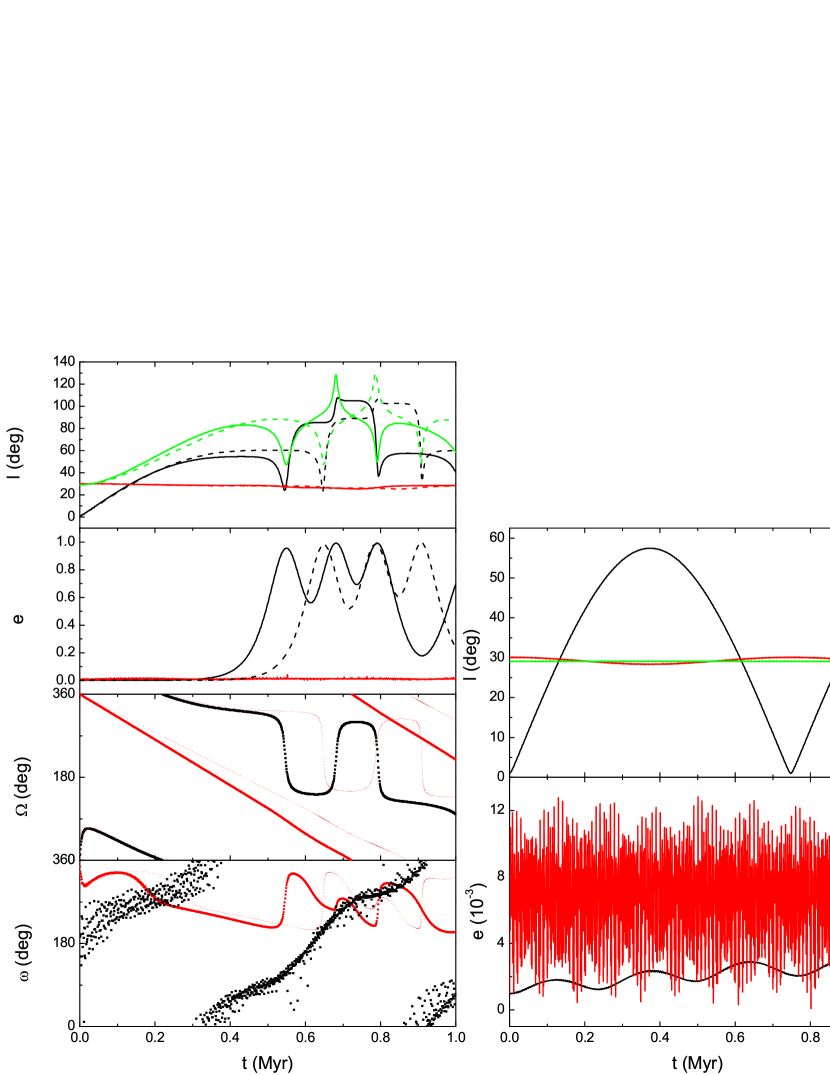
Figure 1: Evolutions of two planets with (left panels) / without (right) an outside disk’s gravity. The initial conditions are listed in Table 1. Black lines are for the inner planet, and red for the outer one. Green lines in the top panels indicate the mutual inclination of two planets. Dash lines in the two left-upper panels and lighter dots in the two left-lower panels are the results of the evolution equations (8).

References

- Albrecht et al. (2012) Albrecht, S.,Winn, J.N.,Johnson, J.A.,et al. 2012, ApJ, 757, 18
- Brown et al. (2012) Brown, D.J.A., Cameron,A.C.,Anderson, D.R.,et al. 2012, MNRAS, 423,1503
- Fabrycky & Tremaine (2007) Fabrycky, D., & Tremaine, S. 2007, ApJ, 669, 1298
- Haishch et al. (2001) Haisch, K.E.J.,Lada, E.A.,& Lada, C.J. 2001,ApJ, 553, L153
- Ida & Lin (2004) Ida, S.,& Lin, D.N.C. 2004, ApJ, 604, 388
- Ida et al. (2008) Ida, S.,& Lin, D.N.C. 2008, ApJ, 673, 487
- Innanen et al. (1997) Innanen, K.A., Zheng, J.Q.,Mikkola,S. Valtonen,M.J, 1997,AJ, 113, 1915
- Kozai (1962) Kozai, Y. 1962, AJ, 67, 591
- Kraus & Ireland (2012) Kraus, A.,L., & Ireland, M.,J. 2012, ApJ, 745, 5
- Lidov (1962) Lidov, M.-L. 1962, Planet. Space Sci., 9, 719
- Lin & Papaloizou (1986) Lin, D.N.C., & Papaloizou, J.C.B. 1986, ApJ, 309, 846L
- Lin et al. (1996) Lin, D.N.C.,Bodenheimer, P., & Richardson, D. C. 1996, Nature, 380, 606L
- Lithwick & Naoz (2011) Lithwick, Y., & Naoz, S.,2011, ApJ, 742,94
- Lithwick & Wu (2011) Lithwick, Y., & Wu, Y. 2011, ApJ, 739,31
- Mardling & Lin (2002) Mardling, R., & Lin, D.N.C. 2002, ApJ, 573, 829
- McLaughlin (1924) McLaughlin, D. B. 1924, ApJ, 60, 22
- Murray & Dermott (1999) Murray, C.D., & Dermott, S.F. 1999, Solar system dynamics (Cambridge Univ. Press)
- Nagasawa et al. (2000) Nagasawa, M.,Tanaka, H., & Ida, S. 2000a, AJ, 119, 1480
- Nagasawa & Ida (2000) Nagasawa, M., & Ida, S. 2000b, AJ, 120, 3311
- Nagasawa et al. (2003) Nagasawa, M., Lin,D.N.C, & Ida, S. 2003,ApJ, 586, 1374
- Nagasawa et al. (2008) Nagasawa, M., Ida, S., & Bessho, T. 2008, ApJ, 678, 498
- Naoz et al. (2011a) Naoz, S.,Farr, W.M.,Lithwick, Y.,Rasio, F.A., & Teyssandier, J. 2011a, Nature, 473, 187
- Naoz et al. (2011b) Naoz, S.,Farr, W.M.,Lithwick, Y.,Rasio, F.A., & Teyssandier, J. 2011b, ApJ, submitted, arXiv: 1107.2414v1
- Rossiter (1924) Rossiter, R. A. 1924, ApJ, 60, 15
- Takeda et al. (2008) Takeda, G.,Kita, R., & Rasio,F. A. 2008, ApJ, 683, 1063
- Terquem et al. (2010) Terquem, C.,& Ajmia, A. 2010, MNRAS, 404, 409
- Teyssandier et al. (2012) Teyssandier, J., Terquem, C., & Papaloizou,J.C.B. 2013, MNRAS, 428, 658
- Triaud et al. (2010) Triaud, A.H.M.J., Cameron,A.C., Queloz, D.,et al. 2010, A&A, 524, A25
- Williams & Cieza (2011) Williams, J.,P., & Cieza, L., A. 2011, ARA&A, 49,67
- Winn et al. (2010) Winn, J.N., Fabrycky, D., Albrecht, S. & Johnson, J.A. 2010, ApJ, 718, L145
- Wu & Murray (2003) Wu, Y., & Murray, N. 2003, ApJ, 589, 605
- Wu et al. (2007) Wu, Y., Murray, N.W., & Ramsahai, J.M. 2007, ApJ, 670,820
- Wu & Lithwick (2011) Wu, Y., & Lithwick, Y. 2011, ApJ, 735, 109
- Zhang et al. (2008) Zhang, H.,Yuan, C., Lin, D.N.C., & Yen, D.C.C. 2008, ApJ, 676, 639
- Zhang & Zhou (2010a) Zhang,H.& Zhou,J.-L. 2010a, ApJ, 714,532
- Zhang & Zhou (2010b) Zhang,H.& Zhou,J.-L. 2010b, ApJ, 719,671
- Zhao et al. (2011) Zhao, G., Xie, J.-W., Zhou,J.-L., & Lin,D.N.C. 2012, ApJ, 749, 172