Steady-state fingering patterns for a periodic Muskat problem

Abstract.

We study global bifurcation branches consisting of stationary solutions of the Muskat problem. It is proved that the steady-state fingering patterns blow up as the surface tension increases: we find a threshold value for the cell height with the property that below this value the fingers will touch the boundaries of the cell when the surface tension approaches a finite value from below; otherwise, the maximal slope of the fingers tends to infinity.

1. Introduction

Proposed in $1934$ by Muskat (cf. [11]), the Muskat problem describes the evolution of the interface between to immiscible fluids in a porous medium. In the recent investigation [6] this problem was studied in a new, periodic, setting incorporating gravity, viscosity, and surface tension effects. The current note aims at an in-depth description of the stationary solutions found in that work.

When a heavier viscous fluid rests upon a lighter one, the interface between them is in general not stable; depending on the different densities, and the surface tension, one expects the upper fluid to, at least partially, sink into the lower one, and vice versa. Due to their resemblance to an outstretched hand reaching into a viscous fluid, the resulting shapes are often referred to as fingering patterns. The investigation of such, in different settings, has brought a lot of attention (see, e.g., the pioneering paper [15] and the later investigations [4, 10, 13, 14].

In [6] smooth branches of stationary, i.e. time-independent, solutions of the Muskat problem were found. They are periodic solutions of the Laplace-Young equation under a volume constrain (see (2.3)). The Laplace-Young equation is also known as the capillarity equation and, subjected to boundary constrains, has been studied by many authors (see [7] and the literature therein).

The solutions we found are all even, but only in a small neighbourhood of the trivial solutions can one via linearisation obtain an approximate picture of the fingering patterns. This is due to the fact that global bifurcation theorems are inherently implicit in nature, and thus have the drawback of not disclosing the behaviour of the bifurcation branches away from the bifurcation point. In our present work, we therefore take advantage of the theory for ordinary differential equations and certain symmetry properties of the solutions to give a precise description of the solutions found in [6]: we show that each global bifurcation branch consists entirely of steady-state solutions of minimal period $2\pi/l$, $l\in{\mathbb{N}}$, and that the symmetric fingers described by the interface i) either approach the bottom and the upper boundary of the cell, or ii) display blow-up in the $C^{1}-$norm, while the surface tension coefficient tends from below to a finite value.

The plan is as follows. In Section 2 we give the necessary mathematical background of the problem, and show that, for stationary solutions, it may be reduced to an ordinary differential equation with an additional non-local constraint. The proof of the main result mentioned above is based on the study of the odd solutions of this equation, and the one-to-one correspondence between the odd and the even solutions thereof. This is done in the Section 3, and there we also show that there exist infinitely many global bifurcation branches consisting of odd solutions of the problem. In addition, we describe the behaviour of the steady fingers away from the set of trivial solutions. Finally, it is interesting to see that the steady-state fingering patterns we obtained correspond to certain solutions of the mathematical pendulum. This correspondence is shown in the Appendix.

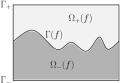
Figure 1. The periodic and vertical Hele-Shaw cell.

2. Preliminaries

Let $h>0$, and consider a periodic medium occupying $\mathbb{S}\times[-h,h]$, with $\mathbb{S}$ denoting the unit circle. The bottom of this cell is assumed to be impermeable, and the pressure on the upper boundary is constantly set to zero. For a function $f$ with $\|f\|_{C(\mathbb{S})}<h$, let

$$\Gamma(f(t)):=\{(x,f(t,x))\,:\,x\in\mathbb{S}\},$$

be the time-dependent interface separating the wetting phases, and $\Gamma_{\pm}:=\mathbb{S}\times\{\pm h\}$ the bottom and the upper boundary of the cell (see Figure 1). We define the fluid domains

$$\Omega_{-}(f(t)) :=\{(x,y)\,:\,-h<y<f(t,x)\},$$

$$\Omega_{+}(f(t)) :=\{(x,y)\,:\,f(t,x)<y<h\},$$

and write

$$\kappa_{\Gamma(f)}:=\frac{f_{xx}}{\left(1+{f_{x}^{2}}\right)^{3/2}}$$

for the signed curvature of the graph $\Gamma(f)$. The mathematical model can then be stated as a two-phase moving-boundary problem,

$$\left\{\begin{array}[]{rlllll}\Delta u_{\pm}&=&0&\text{in}&\Omega_{\pm}(f(t)),\\[8.61108pt] \partial_{\nu}u_{+}&=&g_{1}&\text{on}&\Gamma_{+},\\[8.61108pt] u_{-}&=&g_{2}&\text{on}&\Gamma_{-},\\[8.61108pt] u_{+}-u_{-}&=&\gamma\kappa_{\Gamma(f)}+g(\varrho_{+}-\varrho_{-})f&\text{on}&\Gamma(f(t)),\\[8.61108pt] \partial_{t}f&=&-\displaystyle{\frac{\sqrt{1+f_{x}^{2}}}{\mu_{\pm}}\partial_{\nu}u_{\pm}}&\text{on}&\Gamma(f(t)),\\[8.61108pt] f(0)&=&f_{0},&\end{array}\right.$$ (2.1)

with $t\in[0,T],$ where we use the subscripts $\pm$ to denote the upper and lower fluids, respectively. As conventional, $g$ stands for the gravitational constant of acceleration, $\gamma$ denotes the surface tension at the interface $\Gamma(f)$, and $\varrho_{\pm}$ and $\mu_{\pm}$ are the densities and viscosities of the two fluids, respectively, all of which are supposed to be given positive constants. Physically, the potentials $u_{\pm}$ are defined by the relation

$$u_{\pm}:=p_{\pm}+g\varrho_{\pm}y,$$

where $p$ stands for pressure, and $y$ is the height coordinate. Furthermore, the functions $g_{1}$ and $g_{2}$ are assumed to be known

$$g_{1}\in C([0,T],h^{1+\alpha}(\mathbb{S})) g_{2}\in C([0,T],h^{2+\alpha}(\mathbb{S}))$$ and .

Given $m\in{\mathbb{N}}$ and $\alpha\in(0,1),$ the small Hölder spaces $h^{m+\alpha}(\mathbb{S})$ stand for the completions of the class of smooth functions in the Banach spaces $C^{m+\alpha}(\mathbb{S}).$

The problem consists of finding functions $f$ and $u_{\pm}$ satisfying (2.1), but it can be shown that this may be reduced to a parabolic problem with $f$ as the single unknown [6]. Hence, we shall refer to the function $f$ parametrising the moving interface between the fluids as a solution of (2.1).

Well-posedness results

It is shown in [6] that the Muskat problem is, at least in a neighbourhood of some flat interface, of parabolic type. This observation is true, when considering surface tension effects, independently of the boundary data $g_{1}$ and $g_{2}$. On the other hand, when neglecting surface tension, certain restrictions must be imposed on the boundary data to ensure parabolicity of (2.1). We then have (cf. [6, Theorem 2.1]):

Theorem 2.1 (Well-posedness).

Let $\gamma\in[0,\infty)$, $c_{1},c_{2}\in\mathbb{R}$, and assume that

$$\gamma>0\qquad\text{or}\qquad g(\rho_{+}-\rho_{-})+c_{1}\left(\frac{\mu_{-}}{\mu_{+}}-1\right)<0.$$ (2.2)

Then there exist open neighbourhoods of the zero function $\mathcal{O}_{i}\subset h^{i+\alpha}(\mathbb{S})$, $i\in\{1,2\},$ and $\mathcal{O}\subset h^{2+2\mathop{\rm sign}\nolimits(\gamma)+\alpha}(\mathbb{S})$, such that for all $f_{0}\in\mathcal{O}$ and $g_{i}\in C([0,\infty),c_{i}+\mathcal{O}_{i}),$ $i=1,2,$ there exists $T(f_{0})\leq T$ and a unique maximal Hölder solution $f$ of problem (2.1) on $[0,T(f_{0}))$ which fulfills $f(t)\in\mathcal{O}$ for all $t\in[0,T(f_{0})).$

If $\gamma>0$, then we may choose $\mathcal{O}_{i}=h^{i+\alpha}(\mathbb{S})$, $i\in\{1,2\}.$

Existence of classical solutions of the Muskat problem, and long-time existence for small initial data, can also be found in [8, 16, 17, 18]. The approach in [6] yields structural insight into the character of the Muskat and it is suitable for studying the stability properties of the steady-state solutions of problem (2.1).

Steady-state solutions

In the remainder of this paper we assume that $g_{1}\equiv 0$ and $g_{2}\equiv{\rm const},$ meaning that the mass of both fluids is preserved in time, and that the cell contains equal quantities of both fluids. The steady-state solutions of (2.1) are then solutions of the problem

$$\gamma\frac{f^{\prime\prime}}{(1+f^{\prime 2})^{3/2}}+g(\varrho_{+}-\varrho_{-})f=const,\quad\text{and}\quad\int_{\mathbb{S}}f\,dx=0.$$ (2.3)

Indeed, since $f$ does not depend on time, it follows from uniqueness for the Dirichlet–Neumann problem that the potentials $u_{+}$ and $u_{-}$ are both constants also in the spatial variable, which yields the first equation of (2.3). The second relation reflects the earlier mentioned assumption that the cell contains equal amounts of both fluids. By induction, we obtain

Remark 2.2.

Any classical solution of (2.3) is smooth.

We shall refer to the set

$$\Sigma:=\{(\gamma,0)\,:\,\gamma>0\}$$

as being the trivial branch of solutions of (2.3). Because of the integral constraint in (2.3), the problem (2.3) is in general over-determined. One way to approach this difficulty is to determine solution pairs $(\gamma,f)\in(0,\infty)\times C^{2}(\mathbb{S})$ of (2.3), under the additional, but natural, requirement that $\|f\|_{C(\mathbb{S})}<h$, meaning that the fingers do not touch the lower or upper boundaries of the cell.

In the situation when the less dense fluid lies on the bottom of the cell, i.e. when $\varrho_{+}>\varrho_{-}$, we find—using the theorem on bifurcation from simple eigenvalues due to Crandall and Rabinowitz [3, Theorem 1.7], and the global bifurcation theorem due to Rabinowitz [9, Theorem II.3.3]—global bifurcation branches consisting of even, stationary, finger-shaped solutions of (2.3). More precisely, if $C^{3+\alpha}_{0,e}(\mathbb{S})$ denotes the subspace of $C^{3+\alpha}(\mathbb{S})$ consisting of even functions with integral mean zero, and

$$\mathcal{W}:=\left\{f\in C^{3+\alpha}_{0,e}(\mathbb{S})\,:\,\|f\|_{C(\mathbb{S})}<h\right\},$$

we have (cf. [6, Theorem 6.1 and Theorem 6.3]):

Theorem 2.3 (Bifurcation of stationary solutions).

Let $g_{1}\equiv 0$, $g_{2}\equiv{\rm const},$ and $\varrho_{+}>\varrho_{-}$, $1\leq l\in{\mathbb{N}}$. The point

$$(\overline{\gamma}_{l},0):=(g(\varrho_{+}-\varrho_{-})/l^{2},0)$$ (2.4)

belongs to the closure $\mathcal{S}$ of the set of nontrivial solutions of (2.3) in $(0,\infty)\times\mathcal{W}.$ Denote by $\mathcal{C}_{l}$ the connected component of $\mathcal{S}$ to which $(\overline{\gamma}_{l},0)$ belongs. Then $\mathcal{C}_{l}$ has, in a neighbourhood of $(\overline{\gamma}_{l},0),$ an analytic parametrisation $(\gamma_{l},f_{l}):(-\delta,\delta)\to(0,\infty)\times\mathcal{W}$,

$$\gamma_{l}(\varepsilon) =\overline{\gamma}_{l}+\frac{3g(\varrho_{+}-\varrho_{-})}{8}\varepsilon^{2}+O(\varepsilon^{3}),$$

$$f_{l}(\varepsilon) =\varepsilon\cos(lx)+O(\varepsilon^{2}),$$

as $\varepsilon\to 0.$ Any other pair $(\gamma,0)$, $\gamma>0$, belongs to a neighbourhood in $(0,\infty)\times\mathcal{W}$ with only trivial solutions of (2.3).

Furthermore, if $\varepsilon$ is small and $\gamma=\gamma_{l}(\varepsilon),$ then $f_{l}(\varepsilon)$ is an unstable stationary solutions of (2.1).

Theorem 2.3 is obtained by differentiating the first relation of (2.3) and finding in this way an equation for $f$ only (this is why solutions in $C^{3+\alpha}_{0,e}(\mathbb{S})$ are considered). It is not difficult to show that if $\varrho_{-}\geq\varrho_{+},$ then (2.3) has only the trivial solution $f=0$ (see, e.g., [5]). In the paper at hand we show (cf. Remark 4.3) that this is the case when $\varrho_{-}<\varrho_{+}$ too, as long as the surface tension coefficient is large enough.

3. Odd steady-state fingering solutions

In this section we consider the odd solutions of (2.3). If $f$ is an odd function on $\mathbb{S}$, then $f$ has integral mean $0$ and $f(0)=f^{\prime\prime}(0)=0$. Hence, the odd steady states of the Muskat problem (2.1) are exactly the odd solutions of the equation

$$\frac{f^{\prime\prime}}{(1+f^{\prime 2})^{3/2}}+\lambda f=0,\qquad\lambda>0,$$ (3.1)

within the set

$$\mathcal{U}:=\left\{f\in C^{\infty}(\mathbb{S})\colon\|f\|_{C(\mathbb{S})}<h\right\}.$$

Here, the shorthand

$$\lambda:=\frac{g(\varrho_{+}-\varrho_{-})}{\gamma},$$ (3.2)

indicates the character of (3.1) as an eigenvalue problem. Notice that, throughout this work, we consider the unstable case when $\varrho_{+}>\varrho_{-}$, i.e. when the heavier fluid occupies the upper part of the membrane. Equation (3.1) admits the following scaling property:

Proposition 3.1.

If $(\gamma,f)$ defines a solution of (3.1) through (3.2), then

$$\left(l^{-2}\gamma,l^{-1}f(l\cdot)\right),\qquad l\in{\mathbb{N}},$$ (3.3)

is also a solution of (3.1).

Proof.

Since $\lambda$ is inversely proportional to $\gamma$, the result is immediate. ∎

The main result of this work is the following theorem, which states that a global bifurcation branch consisting of odd functions of minimal period $2\pi$ emanates from the trivial branch of solutions $\Sigma$ at $(\overline{\gamma}_{1},0),$ where $\overline{\gamma}_{1}$ is defined by (2.4). This will later be used to characterise the global bifurcation branches of odd solutions which arise at $(\overline{\gamma}_{l},0),l\geq 2,$ (see Corollary 3.3 below), and in Section 4 to describe the global bifurcation branches $\mathcal{C}_{l}$ obtained in Theorem 2.3.

Recall the definition of the beta function,

$$B(x,y):=\int_{0}^{1}t^{x-1}(1-t)^{y-1}\,dt,\qquad\mathop{\rm Re}\nolimits x,\mathop{\rm Re}\nolimits y>0.$$

Theorem 3.2.

For each $h>0$, there exists

$$\lambda_{h}\geq\lambda_{*}:=\frac{1}{2\pi^{2}}\left(B\left(\textstyle{\frac{3}{4},\frac{1}{2}}\right)\right)^{2},$$ (3.4)

and corresponding $\gamma_{h}\leq\gamma_{*}$ defined by (3.2), with the property that the nontrivial odd solutions of (3.1) of minimal period $2\pi$ within $\mathcal{U}$ coincide with the global bifurcation curve

$$\Sigma_{1}:=\{(\gamma,\pm f_{\gamma})\,:\,\gamma\in(\overline{\gamma}_{1},\gamma_{h})\},$$

where the odd function $f_{\gamma}\in C^{\infty}(\mathbb{S})$ is uniquely determined by the parameter $\gamma\in(\overline{\gamma}_{1},\gamma_{*})$ if we require that $f_{\gamma}^{\prime}(0)\geq 0.$ Let $h_{*}:=\sqrt{2/\lambda_{*}}$, and let $f_{\gamma}$ denote the solution of (3.1) of minimal period $2\pi$ (not necessarily in $\mathcal{U}$). The mapping $(\overline{\gamma}_{1},\gamma_{*})\times\mathbb{S}\ni(\gamma,x)\mapsto f_{\gamma}(x)$ is smooth, and

• if $h<h_{*}$, then $\gamma_{h}<\gamma_{*}$, and

  $$\|f_{\gamma}\|_{C(\mathbb{S})}=f_{\gamma}(\pi/2)\nearrow h\quad\text{ as }\quad\gamma\nearrow\gamma_{h};$$

• if $h=h_{*}$, then $\gamma_{h}=\gamma_{*}$, and

  $$\|f_{\gamma}\|_{C(\mathbb{S})}=f_{\gamma}(\pi/2)\nearrow h,\qquad\|f_{\gamma}^{\prime}\|_{C(\mathbb{S})}=f^{\prime}_{\gamma}(0)\nearrow\infty\quad\text{ as }\quad\gamma\nearrow\gamma_{h};$$

• if $h>h_{*}$, then $\gamma_{h}=\gamma_{*}$, and

  $$\|f_{\gamma}^{\prime}\|_{C(\mathbb{S})}=f^{\prime}_{\gamma}(0)\nearrow\infty\quad\text{ as }\quad\gamma\nearrow\gamma_{h},$$

  while $\sup_{[\overline{\gamma}_{1},\gamma_{*})}\|f_{\gamma}\|_{C(\mathbb{S})}<h$.

Recall that $\overline{\gamma}_{l},$ $1\leq l\in{\mathbb{N}},$ is the constant defined by (2.4). Combining Proposition 3.1 and Theorem 3.2 we conclude:

Corollary 3.3.

Let $2\leq l\in{\mathbb{N}}$. There exists $\gamma_{l,h}\in(\overline{\gamma}_{1},\gamma_{*}]$ with the property that

$$\Sigma_{l}:=\left\{(l^{-2}\gamma,\pm l^{-1}f_{\gamma}(l\cdot))\,:\,\gamma\in(\overline{\gamma}_{1},\gamma_{l,h})\right\}$$

consists exactly of the nontrivial odd solutions of minimal period $2\pi/l$ of (3.1) within $\mathcal{U}.$ The alternatives $(i)-(iii)$ of Theorem 3.2 hold true with the natural modifications. The disjoint union

$$\mathcal{S}_{2\pi}:=\left(\cup_{l=1}^{\infty}\Sigma_{l}\right)\cup\left(\cup_{l=1}^{\infty}\left[\left(\overline{\gamma}_{l+1},\overline{\gamma}_{l}\right)\times\{0\}\right]\right)\cup\left[(\overline{\gamma}_{1},\infty)\times\{0\}\right]$$ (3.5)

constitutes all nontrivial $2\pi-$periodic and odd solutions of (3.1) in $\mathcal{U}$.

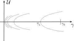
Figure 2. A qualitative picture of the $2\pi$-periodic solutions described in Corollary 3.3.

Remark 3.4.

Put differently, Corollary 3.3 states that global bifurcation branches consisting of odd solutions emanate from $\Sigma$ at $\overline{\gamma}_{l},$ $1\leq l\in{\mathbb{N}}$. Moreover, these bifurcation branches are pairwise disjoint.

Remark 3.5.

It is worth mentioning that, for the same $\gamma$, we may find $2\pi$-periodic odd solutions of (3.1) of different minimal periods (see Figure 2). Since $\gamma_{l,h}=\gamma_{*}>\overline{\gamma}_{1}$, for $l$ large enough, there exists positive integers $l\in{\mathbb{N}},$ such that

$$\overline{\gamma}_{l+1}<\overline{\gamma}_{l}<\frac{\gamma_{*}}{(l+1)^{2}}<\frac{\gamma_{*}}{l^{2}}.$$

Consequently equation (3.1) possesses a solution which belongs to $\Sigma_{l}$ and another one in $\Sigma_{l+1},$ corresponding to the same $\gamma$.

In order to prove Theorem 3.2 we need some preliminary results.

Proposition 3.6.

Let $\lambda>0$ and $\alpha\in{\mathbb{R}}$ be given. The initial-value problem

$$\left\{\begin{array}[]{rllll}\displaystyle\frac{f^{\prime\prime}}{(1+f^{\prime 2})^{3/2}}+\lambda f&=&0&\text{on}&\mathbb{S},\\[4.30554pt] f(0)&=&0,\\[4.30554pt] f^{\prime}(0)&=&\alpha\end{array}\right.$$ (3.6)

possesses a unique classical solution $f_{\lambda,\alpha}$. The solution is odd and periodic in $x$, and smooth as a map

$$(0,\infty)\times{\mathbb{R}}\times{\mathbb{R}}\mapsto f_{\lambda,\alpha}(x).$$

Proof.

Setting $g:=f^{\prime}$, we rewrite (3.6) as an initial value problem for the pair $(f,g),$

$$\left(\begin{array}[]{c}f\\ g\end{array}\right)^{\prime}=F\left(\begin{array}[]{c}f\\ g\end{array}\right),\quad\left(\begin{array}[]{c}f\\ g\end{array}\right)(0)=\left(\begin{array}[]{c}0\\ \alpha\end{array}\right),$$ (3.7)

where $F:{\mathbb{R}}^{2}\to{\mathbb{R}}^{2}$ is defined by

$$F\left(\begin{array}[]{c}f\\ g\end{array}\right)=\left(\begin{array}[]{c}g\\ -\lambda f(1+g^{2})^{3/2}\end{array}\right).$$

Since $F$ is smooth, there is a unique and smooth solution of (3.7), defined on a maximal interval $[0,T)$; if $T<\infty$, then the solution blows up, meaning that $\sup_{[0,T)}|(f,g)|=\infty$ (cf. [1]).

Notice that if $f$ is an odd solution of (3.1) with slope $f^{\prime}(0)=\alpha>0$, then $-f$ is also an odd solution of (3.1) with slope $-\alpha$. Without loss of generality we may therefore restrict our attention to solutions of (3.1) with nonnegative slope at $x=0$. Clearly, the solution of (3.6) with slope $\alpha=0$ is $f\equiv 0$.

Suppose now that $\alpha>0$. We prove that there exists a positive constant $\theta_{\lambda,\alpha}$ such that $f^{\prime}>0$ on $[0,\theta_{\lambda,\alpha})$ and $f^{\prime}(\theta_{\lambda,\alpha})=0.$ Indeed, assuming the contrary, we obtain in view of $f^{\prime}(0)=\alpha>0$, that $f^{\prime}>0$ on $[0,T)$.

On the one hand, if $T=\infty$, we infer from (3.1) that

$$0=f^{\prime\prime}(x)+\lambda f(x)\left(1+(f^{\prime}(x))^{2}\right)^{3/2}\geq f^{\prime\prime}(x)+\lambda f(1),\quad\text{for all }\quad x\geq 1.$$

Integration yields that

$$f^{\prime}(x)\leq f^{\prime}(1)-\lambda f(1)(x-1)\to-\infty\quad\text{ as }\quad x\to\infty,$$

which contradicts our assumption.

On the other hand, if $T<\infty,$ then either $\sup_{[0,T)}f=\infty$ or $\sup_{[0,T)}f^{\prime}=\infty$, the latter case being excluded by the fact that $f^{\prime}$ is decreasing for positive $f$. If $\sup_{[0,T)}f=\infty$, we multiply (3.1) by $-f^{\prime}$ and integrate over $[0,x]$ to obtain that

$$\frac{1}{(1+f^{\prime 2}(x))^{1/2}}=\frac{1}{(1+\alpha^{2})^{1/2}}+\frac{\lambda f^{2}(x)}{2},\qquad 0<x<T.$$ (3.8)

Letting $x\to T$, we obtain the desired contradiction. Consequently, there exists a unique $\theta_{\lambda,\alpha}>0$, such that $f^{\prime}>0$ on $[0,\theta_{\lambda,\alpha})$ and $f^{\prime}(\theta_{\lambda,\alpha})=0.$

It can be easily seen that $f$ extends to an odd function of minimal period $T_{\lambda,\alpha}:=4\theta_{\lambda,\alpha}$. Indeed, we see that

$$f_{\lambda,\alpha}(x):=\left\{\begin{array}[]{rllll}f(x),&&0\leq x\leq\theta_{\lambda,\alpha},\\[4.30554pt] f(2\theta_{\lambda,\alpha}-x),&&\theta_{\lambda,\alpha}\leq x\leq 2\theta_{\lambda,\alpha},\\[4.30554pt] -f(x-2\theta_{\lambda,\alpha}),&&2\theta_{\lambda,\alpha}\leq x\leq 3\theta_{\lambda,\alpha},\\[4.30554pt] -f(4\theta_{\lambda,\alpha}-x),&&3\theta_{\lambda,\alpha}\leq x\leq 4\theta_{\lambda,\alpha},\end{array}\right.$$ (3.9)

has an odd and $T_{\lambda,\alpha}-$periodic extension on the whole of ${\mathbb{R}}$. ∎

We now explicitly determine the minimal period, called $T_{\lambda,\alpha}$, of the solution $f_{\lambda,\alpha}$ of (3.6). In order to simplify calculations, we put

$$\beta:=\frac{1}{\sqrt{1+\alpha^{2}}}.$$

From relation (3.8), we find for $x=\theta_{\lambda,\alpha}$ that the maximum of $f_{\lambda,\alpha}$ is

$$f_{\lambda,\alpha}(\theta_{\lambda,\alpha})=\sqrt{2\lambda^{-1}\left(1-\beta\right)}.$$ (3.10)

We also infer from the same relation that

$$f_{\lambda,\alpha}^{\prime}(x)=\sqrt{\left(\beta+\frac{\lambda f^{2}_{\lambda,\alpha}(x)}{2}\right)^{-2}-1}\quad\text{ for all $x\in[0,\theta_{\gamma,\alpha}]$.}$$

Dividing this equality by its right-hand side, we find that

$$\theta_{\lambda,\alpha}=\int_{0}^{\theta_{\lambda,\alpha}}f_{\lambda,\alpha}^{\prime}(x)\left(\left(\beta+\frac{\lambda f^{2}_{\lambda,\alpha}(x)}{2}\right)^{-2}-1\right)^{-1/2}\,dx,$$

and the variable substitution $f(x)=s$ yields

$$\theta_{\lambda,\alpha}=\int_{0}^{f_{\lambda,\alpha}(\theta_{\lambda,\alpha})}\left(\left(\beta+\frac{\lambda s^{2}}{2}\right)^{-2}-1\right)^{-1/2}\,ds.$$

Finally, setting $\tau:=s/f_{\lambda,\alpha}(\theta_{\lambda,\alpha})$, we obtain in virtue of (3.10) that

$$\theta_{\lambda,\alpha}=\sqrt{\frac{2}{\lambda}}\int_{0}^{1}\frac{(1-\beta)\tau^{2}+\beta}{\sqrt{(1-\tau^{2})\left[1+(1-\beta)\tau^{2}+\beta\right]}}\,d\tau,$$ (3.11)

for all $\alpha,\lambda>0.$ Since $\alpha\mapsto\beta$ is smooth, we may extend $\theta_{\lambda,\alpha}$ continuously to $(0,\infty)\times[0,\infty)$. More precisely, we state:

Lemma 3.7.

The function $\theta_{\lambda,\alpha}$ defined in (3.11),

$$(0,\infty)\times[0,\infty)\ni(\lambda,\alpha)\mapsto\theta_{\lambda,\alpha}\in(0,\infty),$$

is smooth, and strictly decreasing with respect to both $\lambda$ and $\alpha$. Moreover

$$\theta_{\lambda,0}=\frac{\pi}{2\sqrt{\lambda}}\qquad\text{and}\qquad\lim_{\alpha\nearrow\infty}\theta_{\lambda,\alpha}=\frac{1}{2\sqrt{2\lambda}}\,B\left(\frac{3}{4},\frac{1}{2}\right).$$ (3.12)

Proof.

The integral on the right-hand side of (3.11) exists because the singularity behaves like ${(1-\tau)^{-1/2}}$ as $\tau\to 1$. Therefrom, the regularity assertion is clear. Let us now show that $\theta_{\lambda,\alpha}$ is strictly decreasing with respect to $\alpha$. To this aim we fix $\tau\in(0,1)$ and define the function

$$g_{\tau}(\alpha) :=(1-\beta)\tau^{2}+\beta$$

$$=(1-(1+\alpha^{2})^{-1/2})\tau^{2}+(1+\alpha^{2})^{-1/2},\qquad\alpha\geq 0.$$

Since

$$\theta_{\lambda,\alpha}=\sqrt{\frac{2}{\lambda}}\int_{0}^{1}\frac{1}{\sqrt{1-\tau^{2}}}\frac{g_{\tau}(\alpha)}{\sqrt{1+g_{\tau}(\alpha)}}\,d\tau,$$

we see that $\theta_{\lambda,\alpha}$ is strictly decreasing with respect to $\lambda$, and it suffices to show that the mapping $\left[[0,\infty)\ni\alpha\mapsto g_{\tau}(\alpha)(1+g_{\tau}(\alpha))^{-1/2}\right]$ has a negative derivative for all $\tau\in(0,1)$, $\alpha>0$. Indeed, since for such $\alpha$ and $\tau$ we have that

$$\frac{\partial g_{\tau}}{\partial\beta}=1-\tau^{2}>0\quad\text{ and }\quad\frac{\partial\beta}{\partial\alpha}=-\frac{\alpha}{(1+\alpha^{2})^{3/2}}<0,$$

it follows from the chain rule that

$$\frac{d}{d\alpha}\left(\frac{g_{\tau}(\alpha)}{1+g_{\tau}(\alpha)}\right)=\frac{g_{\tau}^{\prime}(\alpha)(2+g_{\tau}(\alpha))}{2(1+g_{\tau}(\alpha))^{3/2}}<0,\quad\text{for all $\tau\in(0,1)$.}$$

In view of that $g_{\tau}(0)=1,$ the first equality in (3.12) follows. Taking into consideration that $\lim_{\alpha\to\infty}g_{\tau}(\alpha)=\tau^{2}$, we obtain that

$$\lim_{\alpha\to\infty}\theta_{\lambda,\alpha} =\sqrt{\frac{2}{\lambda}}\int_{0}^{1}\frac{\tau^{2}}{\sqrt{1-\tau^{4}}}\,d\tau=\frac{1}{2\sqrt{2\lambda}}\int_{0}^{1}s^{-1/4}(1-s)^{-1/2}\,ds$$

$$=\frac{1}{2\sqrt{2\lambda}}\,B\left(\frac{3}{4},\frac{1}{2}\right).$$

This completes the proof. ∎

Recall that we are interested in determining the solutions of (3.1) which are not only odd, but also of minimal period $2\pi$. Thus, we are interested in determining the set of $\lambda$ and $\alpha$ such that $\theta_{\lambda,\alpha}=\pi/2$. The following lemma provides an answer in terms of a function $\lambda\mapsto\alpha$.

Lemma 3.8.

Let $\lambda_{*}$ be the constant defined by the relation (3.4). If $\lambda\not\in(\lambda_{*},1]$ then $\theta_{\lambda,\alpha}\neq\pi/2$, but given $\lambda\in(\lambda_{*},1]$ there exists a unique $\alpha(\lambda)\in[0,\infty)$ such that $\theta_{\lambda,\alpha(\lambda)}=\pi/2.$ The mapping

$$(\lambda_{*},1]\ni\lambda\mapsto\alpha(\lambda)\in[0,\infty)$$

is smooth, bijective, and decreasing.

Proof.

In view of Lemma 3.7, we have that $\theta_{\lambda,\alpha}=\pi/2$ if and only if

$$\frac{1}{2\sqrt{2\lambda}}B\left(\textstyle{\frac{3}{4},\frac{1}{2}}\right)<\frac{\pi}{2}\leq\frac{\pi}{2\sqrt{\lambda}},$$

which is equivalent to that $\lambda\in(\lambda_{*},1]$. Since $[(\lambda,\alpha)\mapsto\theta_{\lambda,\alpha}]$ is smooth and $\partial_{\alpha}\theta_{\lambda,\alpha}<0$ for $\alpha>0$, we infer from the implicit function theorem that $[\lambda\mapsto\alpha(\lambda)]$ is smooth as well. Then

$$0=\frac{d}{d\lambda}\theta_{\lambda,\alpha(\lambda)}=\partial_{\lambda}\theta_{\lambda,\alpha}+\left(\partial_{\alpha}\theta_{\lambda,\alpha}\right)\alpha^{\prime}(\lambda),$$

so that $\alpha^{\prime}(\lambda)<0$ for $\lambda\in(\lambda_{*},1)$ in view of Lemma 3.7. From (3.12) we infer that $\alpha(1)=0$ and $\lim_{\lambda\to\lambda_{*}}\alpha(\lambda)=\infty$. ∎

With these preparations done, we come to the proof of the main result as stated in Theorem 3.2:

Proof of Theorem 3.2.

It follows from Proposition 3.6 and Lemma 3.8 that the odd solutions of (3.1) of minimal period $2\pi$ coincide with the set

$$\{(\lambda,\pm f_{\lambda})\,:\,\lambda\in(\lambda_{*},1]\},$$

where we simply write $f_{\lambda}:=f_{\lambda,\alpha(\lambda)}$. In order for those solutions to be physically realistic, we still have to require that $f_{\lambda}\in\mathcal{U}$, i.e. that $\|f\|_{C(\mathbb{S})}<h$. The maximum of $|f_{\lambda}|$ is achieved at $x=\theta_{\lambda,\alpha(\lambda)}=\pi/2$, and we infer from (3.10) that $\lambda\in(\lambda_{*},1]$ must additionally satisfy

$$f_{\lambda}(\pi/2)=\sqrt{2\lambda^{-1}\left(1-(1+\alpha^{2}(\lambda))^{-1/2}\right)}<h.$$ (3.13)

Let us first assume that $h^{2}<2\lambda_{*}^{-1}$. Since, in view of Lemma 3.8,

$$2\lambda^{-1}\left(1-(1+\alpha^{2}(\lambda))^{-1/2}\right)\;\nearrow_{\lambda\to\lambda_{*}}\;2\lambda_{*}^{-1}$$

we find a unique $\lambda_{h}>\lambda_{*}$ with the property that

$$\max\left|f_{\lambda_{h}}\right|=\sqrt{2\lambda_{h}^{-1}\left(1-(1+\alpha^{2}(\lambda_{h}))^{-1/2}\right)}=h.$$

By recalling that $\lambda=g(\varrho_{+}-\varrho_{-})/\gamma$, we infer the main part of the theorem, including $(i)$.

If instead $h^{2}=2\lambda_{*}^{-1}$, then $f_{\lambda}\in\mathcal{U}$ for all $\lambda\in(\lambda_{*},1]$ and Lemma 3.8 implies that

$$|f_{\lambda}|\nearrow_{\lambda\to\lambda_{*}}\sqrt{2/\lambda_{*}},\quad\text{ while }\quad f_{\lambda}^{\prime}(0)=\alpha(\lambda)\nearrow_{\lambda\to\lambda_{*}}\infty.$$

We have thus shown that $(ii)$ is valid, and assertion $(iii)$ follows similarly. ∎

Remark 3.9.

Differentiating relation (3.8) with respect to $\lambda$ and using a maximum principle argument, shows that $f_{\lambda_{1}}>f_{\lambda_{2}}$ on $(0,\pi)$ provided $\lambda_{*}<\lambda_{1}<\lambda_{2}\leq 1.$ The evolution of the solution $f_{\lambda}$ with respect to $\lambda\in(\lambda_{*},1]$ is pictured in Figure 3.

Figure 3. Steady-states $f_{\lambda}$ on $\Sigma_{1}$, $\lambda_{*}<\lambda_{2}<\lambda_{1}<1.$

Proof of Corollary 3.3.

The constant $\gamma_{l,h}$ is defined similarly to $\gamma_{h}$, and ensures that $l^{-1}f_{\gamma}(l\cdot)$ remain in $\mathcal{U}$ for all $\gamma\in[\overline{\gamma}_{1},\gamma_{l,h})$ (see the proof of Theorem 3.2). If $l$ is large enough relation (3.10) shows that $\gamma_{l,h}=\gamma_{*}.$ The relation (3.5) now follows in view of that the global bifurcation branch $\Sigma_{l}$ consists exactly of functions with minimal period $2\pi/l$. ∎

4. Description of the bifurcation branches $\mathcal{C}_{l}$

Let us return to the setting of Theorem 2.3. Define

$$\widetilde{\Sigma}_{l}:=\{(\gamma,f_{\gamma}(\cdot+\pi/2l))\,:\,(\gamma,f_{\gamma})\in\Sigma_{l}\}\cup\{(\overline{\gamma}_{l},0)\},\qquad 1\leq l\in{\mathbb{N}}.$$

Since the functions $f_{\gamma}$ are odd (cf. (3.9)), the smooth curve $\widetilde{\Sigma}_{l}$ consists of even functions. Hence, it must be a subset of the maximal connected component of $\mathcal{S}$ to which $(\overline{\gamma}_{l},0)$ belongs, i.e. $\widetilde{\Sigma}_{l}\subset\mathcal{C}_{l}$. We shall prove that the converse is also true. This means that the branches $\mathcal{C}_{l}$ consist, with the exception of the trivial solution $(\overline{\gamma}_{l},0)$, exactly of even functions with minimal period $2\pi/l$. Theorem 3.2 may be then used to describe the global bifurcation branches $\mathcal{C}_{l}$.

Theorem 4.1.

Given $l\in{\mathbb{N}},l\geq 1,$ we have that $\mathcal{C}_{l}=\widetilde{\Sigma}_{l}$.

Since the even solutions of (2.3) near $(\overline{\gamma}_{l},0)$ lay either on the trivial curve $\Sigma$ or on $\mathcal{C}_{l},$ we conclude that $\widetilde{\Sigma}_{l}$ and $\mathcal{C}_{l}$ coincide in a small neighbourhood of $(\overline{\gamma}_{l},0)$. Hence, at least in small neighbourhood of $(\overline{\gamma}_{l},0)$, the (seemingly) arbitrary constant in (2.3) is zero. Even more holds:

Lemma 4.2.

Let $(\gamma,f)\in(0,\infty)\times\mathcal{W}$ be a solution of (2.3). We then have

$$\frac{f^{\prime\prime}}{(1+f^{\prime 2})^{3/2}}+\lambda f=0\quad\text{in $\mathbb{S}$}.$$

Moreover, if $2\pi/l,l\geq 1,$ is the minimal period of $f,$ then $f(\cdot-\pi/2l)$ is an odd solution of (2.3).

Proof.

Assume by contradiction that we would find a solution $(\gamma,f)\in(0,\infty)\times\mathcal{W}$ of (2.3) such that

$$\frac{f^{\prime\prime}}{(1+f^{\prime 2})^{3/2}}+\lambda f=c\quad\text{in $\mathbb{S}$},$$

with a constant $c\neq 0.$ Let $g:=f-c/\lambda.$ Then $g$ is an even solution of (3.1), but $g$ has no longer integral mean equal to $0$. Since $g^{\prime}(0)=0$, it must hold $g(0)\neq 0.$ Otherwise, $g=0,$ meaning that $f=c/\lambda,$ which contradicts $f\in\mathcal{W}$.

We may, without loss of generality, assume that $g(0)>0$. There exists a positive time $T_{c}>0$ such that $g>0$ on $[0,T_{c})$ and $g(T_{c})=0.$ Indeed, if this is not the case, we infer from (3.1) that $g^{\prime\prime}<0.$ This is in contradiction with the fact that $g$ is periodic. The function $g$ is a $4T_{c}-$periodic function on ${\mathbb{R}},$ since it must hold that

$$g(x)=\left\{\begin{array}[]{rllll}g(x),&&0\leq x\leq T_{c},\\[4.30554pt] -g(2T_{c}-x),&&T_{c}\leq x\leq 2T_{c},\\[4.30554pt] -g(x-2T_{c}),&&2T_{c}\leq x\leq 3T_{c},\\[4.30554pt] g(4T_{c}-x),&&3T_{c}\leq x\leq 4T_{c}.\end{array}\right.$$ (4.1)

Moreover, $g$ is $2\pi-$periodic, so that $T_{c}=\pi/(2k),$ for some $k\in{\mathbb{N}}.$ We conclude that $g$ has integral mean zero, which is in contradiction with $f\in\mathcal{W}$ and $c\neq 0.$ Thus, $f$ must solve (3.1). The relation (4.1) then holds also for $f$, provided that $T_{c}=\pi/2l$. This completes the proof. ∎

In virtue of Corollary 3.3, Proposition 3.6, and the proof of Lemma 4.2 we conclude:

Remark 4.3.

The solutions of (2.3) are, up to translation, odd. Moreover, problem (2.3) has no solutions $(\gamma,f)\in(0,\infty)\times\mathcal{U}$ if $\gamma>\gamma_{h}.$

With this preparation done, the proof of Theorem 4.1 is immediate.

Proof of Theorem 4.1.

Lemma 4.2 shows that the mapping

$$\cup_{l=1}^{\infty}\left(\Sigma_{l}\cup\{(\overline{\gamma}_{l},0)\}\right)\to\mathcal{S},\qquad\Sigma_{l}\cup\{(\overline{\gamma}_{l},0)\}\ni(\gamma,f)\mapsto(\gamma,f(\cdot+\pi/2l)),$$

is one-to-one and onto. Recall that $\mathcal{S}$ is the closure of the set of nontrivial solutions of (2.3) in $(0,\infty)\times\mathcal{W},$ and the union $\cup_{l=1}^{\infty}\left(\Sigma_{l}\cup\{(\overline{\gamma}_{l},0)\}\right)$ is, in virtue of Corollary 3.3, disjoint. The image of $\Sigma_{l}\cup\{(\overline{\gamma}_{l},0)\}$ under this mapping is $\widetilde{\Sigma}_{l},$ hence $\mathcal{C}_{l}=\widetilde{\Sigma}_{l}$. ∎

Appendix

It is clear form Proposition 3.1 and Corrolary 3.3 that the $T-$periodic solutions of (2.3) are exactly the elements of the set

$$\mathcal{S}_{T}:=\left\{f\left(\frac{2\pi}{T}\cdot\right)\,:\,f\in\mathcal{S}_{2\pi}\right\}.$$

The volume constrain in (2.3) for $T-$periodic solutions reads as $\int_{0}^{T}f\,dx=0.$ In view of Remark 4.3 we show that each $T-$periodic solution $f$ of (2.3) corresponds to a unique function $\theta$ describing the evolution of a mathematical pendulum (or the bending of an elastic rod):

$$\theta^{\prime\prime}+\lambda\sin(\theta)=0,$$ (4.2)

cf. also [12]. We set $\lambda:=g/l$, with $l$ denoting the length of the pendulum. We refer to [1, 2] for the deduction of (4.2). Herein, of interest are only the solutions of (4.2) which satisfy

$$|\theta|<\pi/2 \theta(0)=0$$ and . (4.3)

Particularly, solutions of (4.2)-(4.3) are odd. We now state:

Theorem 4.4.

There exists a one-to-one correspondence between the even solutions $f$ of (2.3) and the odd solutions $\theta$ of (4.2)-(4.3).

Given $s\in{\mathbb{R}},$ $\theta(s)$ is the angle between the tangent to $\Gamma(f)$ at $z(s)$ and the $Ox$-axis, with $z:{\mathbb{R}}\to{\mathbb{R}}$ a parametrisation of $\Gamma(f)$ by the arc length.

Proof.

Take first $f$ to be an even solution of (2.3). We define the function $p:{\mathbb{R}}\to{\mathbb{R}}$ by

$$p(x)=\int_{0}^{x}\sqrt{1+f^{\prime 2}(t)}\,dt,\qquad x\in{\mathbb{R}}.$$

This mapping is bijective, and let $z$ denote its inverse. Let $\theta:{\mathbb{R}}\to{\mathbb{R}}$ be given by

$$\theta(s)=\arctan f^{\prime}(z(s)),\qquad s\in{\mathbb{R}}.$$ (4.4)

If $L=p(T),$ then $\theta$ is $L-$periodic. Indeed, we have that

$$L=p(z(s+L))-p(z(s))=\int_{z(s)}^{z(s+L)}\sqrt{1+f^{\prime 2}(t)}\,dt=\int_{z(s)}^{z(s)+T}\sqrt{1+f^{\prime 2}(t)}\,dt,$$

hence $z(s+L)=z(s)+T.$ Being a composition of odd functions, $\theta$ is also odd. Given $s\in{\mathbb{R}}$,

$$\theta^{\prime}(s)=\frac{f^{\prime\prime}(z(s))}{1+f^{\prime 2}(z(s))}z^{\prime}(s)=-\lambda f(z(s))z^{\prime}(s)\sqrt{1+f^{\prime 2}(z(s))}=-\lambda f(z(s)),$$

due to

$$z^{\prime}(s)=\frac{1}{p^{\prime}(z(s))}=\frac{1}{(1+f^{\prime 2}(z(s)))^{1/2}}.$$ (4.5)

Hence

$$\theta^{\prime\prime}(s)=\lambda f^{\prime}(z(s))z^{\prime}(s)=-\lambda\frac{f^{\prime}(z(s))}{\sqrt{1+f^{\prime 2}(z(s))}}=-\lambda\sin(\theta(s)),$$

and $\theta$ is a $L-$periodic solution of (4.2)-(4.3).

Conversely, given $\theta$ solution of (4.2)-(4.3), we let $z:{\mathbb{R}}\to{\mathbb{R}}$ be the function defined by

$$z(s):=\int_{0}^{s}\cos(\theta(t))\,dt,\qquad s\in{\mathbb{R}},$$

and write $p$ for its inverse. Setting $T:=\int_{0}^{L}\cos(\theta(t))\,dt,$ we have that $p(x+T)=L+p(x)$ for all $x\in{\mathbb{R}}.$ It can be then easily verified that $f:{\mathbb{R}}\to{\mathbb{R}},$

$$f(x):=-\frac{\theta^{\prime}(0)}{\lambda}+\int_{0}^{x}\tan(\theta(p(t)))\,dt,\qquad x\in{\mathbb{R}},$$

is a $T-$periodic and even solution of (2.3). ∎

With this observation, our result stated in Theorem 3.2 rewrites for the mathematical pendulum equation as follows:

Corollary 4.5.

There exists a smooth curve $\theta_{\lambda},$ $\lambda\in(\lambda_{*},1],$ consisting of $L_{\lambda}-$periodic solutions of (4.2)-(4.3) with the property that

$$\sup|\theta|=\arctan(\alpha(\lambda)))\nearrow_{\lambda\to\lambda_{*}}\pi/2.$$

Remark 4.6.

It is worth noticing that the period $L_{\lambda}$ of these solutions is strictly decreasing with respect to $\lambda.$ Indeed, it holds that

$$L_{\lambda}=\frac{2}{\sqrt{\lambda}}\int_{-\pi/2}^{\pi/2}\frac{d\theta}{\sqrt{1-\sin^{2}(\arctan(\alpha(\lambda))/2)\sin^{2}(\theta)}},$$

and since $\alpha$ decreases with respect to $\lambda$ we obtain the desired conclusion. Though $L_{\lambda}$ can be calculated in terms of elliptic integrals, it is in general difficult to specify for which solution $\theta$ of (4.2)-(4.3) of period $L>0$ it holds that $z(L)=2\pi,$ that is the corresponding solution of (2.3) has period $2\pi.$ Furthermore, the result stated in Corollary 4.5 can not be obtained via standard bifurcation theorems, since the period of $L_{\lambda}$ must decrease with respect to $\lambda.$ These facts serve as a motivation for our approach.

Acknowledgement

The authors are grateful to the anonymous referee for pointing out some ambiguity in the notation of the preliminary version of the paper.

References

- [1] H. Amann, Ordinary Differential Equations. An Introduction to Nonlinear Analysis, Walter de Gruyter, Berlin, 1990.
- [2] B. Buffoni & J. Toland, Analytic Theory of Global Bifurcation: An Introduction, Princeton, New Jersey, 2003.
- [3] M. G. Crandall & P. H. Rabinowitz, Bifurcation from simple eigenvalues, J. Funct. Anal. 8 (1971), 321–340.
- [4] E. DiBenedetto & A. Friedman, The ill-posed Hele-Shaw model and the Stefan problem for supercooled water, Trans. Amer. Math. Soc., 282 (1984), 183–204.
- [5] J. Escher & B.–V. Matioc, Multidimensional Hele-Shaw flows modeling Stokesian fluids, Math. Methods Appl. Sci., 32 (2009), 577–593.
- [6] J. Escher & B.–V. Matioc, On the parabolicity of the Muskat problem: Well-posedness, fingering, and stability results, Z. Anal. Anwend. 30(2) (2011), 193–218.
- [7] R. Finn, Equilibrium Capillary Surfaces, Springer–Verlag, New York, 1986.
- [8] A. Friedman and Y. Tao, Nonlinear stability of the Muskat problem with capillary pressure at the free boundary. Nonlinear Anal. 53 (2003), 45 – 80.
- [9] H. Kielhöfer, Bifurcation Theory: An Introduction with Applications to PDEs, Springer–Verlag, New York, 2004.
- [10] J. McLean & P. Saffman, The effect of surface tension on the shape of fingers in a Hele Shaw cell, J. Fluid Mech., 102 (1981), 455–469.
- [11] M. Muskat, Two fluid systems in porous media. The encroachment of water into an oil sand, Physics, 5 (1934), 250–264.
- [12] H. Okamoto & M. Shoji, The Mathematical Theory of Permanent Progressive Water-Waves, World Scientific Publishing, 2001.
- [13] F. Otto, Viscous fingering: an optimal bound on the growth rate of the mixing zone, SIAM J. Appl. Math., 57 (1997), 982–990.
- [14] P. G. Saffman, Viscous fingering in Hele-Shaw cells, J. Fluid Mech., 173 (1986), 73–94.
- [15] P. G. Saffman & G. Taylor, The penetration of a fluid into a porous medium or Hele-Shaw cell containing a more viscous liquid, Proc. Roy. Soc. London. Ser. A, 245 (1958), 312–329.
- [16] M. Siegel, R. E. Caflisch & S. Howison, Global Existence, Singular Solutions, and Ill-Posedness for the Muskat Problem, Comm. Pure Appl. Math., 57 (2004), 1374–1411.
- [17] F. Yi, Local classical solution of Muskat free boundary problem, J. Partial Diff. Eqs., 9 (1996), 84–96.
- [18] F. Yi, Global classical solution of Muskat free boundary problem, J. Math. Anal. Appl., 288 (2003), 442–461.