Blind Identification of ARX Models with Piecewise Constant Inputs

Abstract

Blind system identification is known to be a hard ill-posed problem and without further assumptions, no unique solution is at hand. In this contribution, we are concerned with the task of identifying an ARX model from only output measurements. Driven by the task of identifying systems that are turned on and off at unknown times, we seek a piecewise constant input and a corresponding ARX model which approximates the measured outputs. We phrase this as a rank minimization problem and present a relaxed convex formulation to approximate its solution. The proposed method was developed to model power consumption of electrical appliances and is now a part of a bigger energy disaggregation framework. Code will be made available online.

I Introduction

Consider an auto-regressive exogenous input (ARX) model

$$y(t)- a_{1}y(t-1)-\cdots-a_{n_{a}}y(t-n_{a})$$

$$= {b}_{1}u(t-n_{k}-1)+\cdots+{b}_{n_{b}}u(t-n_{k}-n_{b})$$ (1)

with input $u\in\Re$ and output $y\in\Re$. Estimation of this type of model is probably the most common task in system identification and a very well studied problem, see for instance [24]. The common setting is that $\{(y(t),u(t))\}_{t=1}^{N}$ is given and the summed residuals

$$\sum_{t=n}^{N}\left(y(t)-\sum_{k_{1}=1}^{n_{b}}{b}_{k_{1}}u(t-k_{1}-n_{k})-\sum_{k_{2}=1}^{n_{a}}a_{k_{2}}y(t-k_{2})\right)^{2}$$

where $n=\max(n_{a},n_{k}+n_{b})+1$, is minimized to obtain an estimate for $a_{1},\dots,a_{n_{a}},{b}_{1},\dots,{b}_{n_{b}}$. This estimate is often referred to as the least squares (LS) estimate.

In this paper we study the more complicated problem of estimating an ARX model from solely outputs $\{y(t)\}_{t=1}^{N}$. This is an ill-posed problem and it is easy to see that under no further assumptions, it would be impossible to uniquely determine $a_{1},\dots,a_{n_{a}},{b}_{1},\dots,{b}_{n_{b}}$.

We will in this contribution study this problem under the assumption that the input is piecewise constant. This is a rather natural assumption and a problem faced in many identification problems. Consider e.g., the modeling of an electrical appliance where the power consumption is monitored while the appliance is turned on and off. The exact time for when the appliance was turned on and off is not known and neither is the amplitude of the “input”.

It should be noticed that the assumption of a piecewise constant input is not enough to uniquely determine the input or the ARX model. Specifically, we will not be able to decide the input or the ARX coefficients ${b}_{1},\dots,{b}_{n_{b}}$ more than up to a multiplicative scalar. However, for many applications this is sufficient, as we will illustrate in the numerical section.

The task of identifying a model from only outputs is in system identification referred to as blind system identification (BSI). It is known to be a difficult problem and in general ill-posed.

II Background

Our work is motivated by blind system identification which is a fundamental signal processing tool used for identifying a system using only observations of the systems output. Formally, given the output signal of a system, BSI serves as a tool for estimating the unknown inputs and system model [2].

Figure 1: Input-Output Model of a System

Consider the block diagram in Figure 1. Suppose that the system we want to identify is linear. Given only $y$, BSI is used to identify the input $u$ and the system transfer function $H$. In this way, BSI is a method for solving the inverse problem of system identification without input information. Consider now a discrete linear, time-invariant system. Note that we describe the theory in this section for discrete time systems but the continuous time counterpart can be derived in a similar fashion. The output can be written as a convolution model, i.e.,

$$y(t)=u(t)\star h(t)+w(t)$$ (2)

where $\star$ is the convolution operator and $w$ is a noise term. This problem can be transfered to the frequency domain by applying the Fourier transform to get the following system:

$$Y(s)=H(s)U(s)+W(s)$$ (3)

An alternative name for BSI when the system is linear, time-invariant is blind deconvolution. For a known input $u(k)$, a deconvolution process can be applied to $y_{i}(k)$ to approximate $h_{i}(k)$. For instance, using a pseudo-inverse filter which is an approximation of the Weiner filter, the result of deconvolution gives

$$U(s)\approx\frac{Y_{i}(s)H^{\dagger}(s)}{|H(s)|^{2}+C}$$ (4)

where $(\cdot)^{\dagger}$ denotes the pseudo-inverse and $C$ is a constant chosen based on heuristics and serves to prevent amplification of noise [12]. However, we are interested in solving the problem with unknown inputs. When the input is unknown, usually partial information about the statistical properties of $\{u(t)\}$ is required in order to obtain a good approximation of the output $\{y(t)\}$. Further, how the partial information is used in the identification problem plays an important role in the quality of the solution [23].

Typically, system identification requires information on the input and the output of a system in order for the problem to be well-posed and to reconstruct the system itself. However, in many applications, e.g., data communications, speech recognition, image restoration and seismic signal processing, this information is not readily available. Broadly speaking, in all these application areas we can describe the identification problem using the following abstract formulation.

Suppose there is a signal that is transmitted through a ‘channel’ that can be described using a linear, time-invariant model with a single input and $p$ outputs. The input to the system $\{u(t)\}$ results in $N$ of output sequences $\{y_{1}(t)\},\ldots,\{y_{p}(t)\}$. Let $\{h_{1}(t)\},\ldots,\{h_{p}(t)\}$ denote the finite impulse responses (FIR’s) which are of order $K$. As we noted above, a linear, time-invariant system of this type can be described using the convolution model in Equation (2) for each $i\in\{1,\ldots,p\}$, i.e.,

$$y_{i}(t)=u(t)\star h_{i}(t)+w_{i}(t).$$ (5)

This model can be concisely as

$${\bf y}={\bf H}{\bf u}+{\bf w}$$ (6)

where

$${\bf y}:=\begin{bmatrix}{\bf y}_{1}^{\mathsf{T}}&\cdots&{\bf y}_{p}^{\mathsf{T}}\end{bmatrix}^{\mathsf{T}}$$ (7)

with each ${\bf y}_{i}=[y_{i}(1)\;\cdots\;y_{i}(N)]^{\mathsf{T}}$, and

$${\bf u}=\begin{bmatrix}u(-K)&u(-K+1)&\cdots&u(N-1)\end{bmatrix}^{\mathsf{T}}.$$ (8)

The matrix ${\bf H}$ takes the form

$${\bf H}:=\begin{bmatrix}{\bf H}_{1}^{\mathsf{T}}&\cdots&{\bf H}_{p}^{\mathsf{T}}\end{bmatrix}^{\mathsf{T}}$$ (9)

where each ${\bf H}_{i}$ is an $N\times(N+K)$ filtering matrix given by

$${\bf H}_{i}=\begin{bmatrix}h_{i}(K)&\cdots&h_{i}(0)&\cdots&0\\ \vdots&\ddots&&\ddots&\vdots\\ 0&\cdots&h_{i}(K)&\cdots&h_{i}(0)\end{bmatrix}.$$ (10)

Now that the system has been written in this form, we can formulate the BSI or blind deconvolution problem and ask when it has a well-defined solution. If a system identification problem is well-posed, then all the unknown parameters can be uniquely determined given the data. Given ${\bf y}$ and ${\bf w}\equiv 0$, then we can only hope to solve the system in Equation (6) for unique ${\bf u}$ and ${\bf H}$ up to a scalar [2]. In this case we call the system identifiable. Necessary and sufficient conditions for identifiability are given in [21] and summarized in [2].

There are a number of methods for estimating either the input ${\bf u}$ or the system function ${\bf H}$. Once either the input or the system matrix has been estimated, the other can be calculated using the estimate. The application typically determines whether a direct estimation of input or system matrix should be done. For instance, in communication applications the input carries the information and as such direct estimation should be used for the input and the system matrix should be calculated after. The input ${\bf u}$ can be estimated using the following methods: input subspace (IS) method, mutually referenced equalizers (MRE), or linear prediction (LP) method (see [2, 17, 27]). The system matrix can be directly estimated using the maximum likelihood (ML) method (see, for instance, [32]) and the subspace method (see [1]). We remark that in the above formulation we have considered only FIR models. These tend to be sufficient in practice considering that infinite impulse responses can be approximated by FIR’s and modeling with FIR’s results in problem formulations that have tractable solutions.

In this paper we are concerned specifically with estimating an ARX model from only output observations and we formulate the problem using the BSI framework.

III Problem Formulation

Given $\{y(t)\}_{t=1}^{N}\in\Re$ and a bound for the noise $\epsilon$, find an estimate for $a_{1},\dots,a_{n_{a}},{b}_{1},\dots,{b}_{n_{b}}\in\Re$ and an over time piecewise constant $u(t)\in\Re,t=1,\dots,N,$ such that

$$y(t)- a_{1}y(t-1)-\cdots-a_{n_{a}}y(t-n_{a})$$

$$= {b}_{1}u(t-n_{k}-1)+\cdots+{b}_{n_{b}}u(t-n_{k}-n_{b})+w(t),$$

for $t=n,\dots,N$, where $n=\max(n_{a},n_{k}+n_{b})+1$, and

$$|w(t)|\leq\epsilon,\quad t=n,\dots,N.$$ (11)

We will for simplicity assume that $n_{a},n_{b},n_{k},$ are known. To make the problem well posed, we will seek the piecewise constant input with the least amount of changes. Other choices have been studied for the related problem of blind deconvolution, see [3] for a solution where the signals to be recovered are assumed to be in some known subspaces.

IV Notation and Assumptions

We will use $y$ to denote the output and $u$ the input. We will for simplicity only consider single input single output (SISO) systems. We will assume that $N$ measurements of $y$ are available and stack them in the vector ${\bf y}$, i.e.,

$${\bf y}=\begin{bmatrix}{y}(1)&\dots&{y}(N)\end{bmatrix}^{\mathsf{T}}.$$ (12)

We also introduce ${\bf u}$, ${\bf w}$, ${\bf a}$ and ${\bf b}$ as

$${\bf u}= \begin{bmatrix}u(1)&\dots&u(N)\end{bmatrix}^{\mathsf{T}},$$ (13)

$${\bf w}= \begin{bmatrix}w(1)&\dots&w(N)\end{bmatrix}^{\mathsf{T}},$$ (14)

$${\bf a}= \begin{bmatrix}a_{1}&\dots&a_{n_{a}}\end{bmatrix}^{\mathsf{T}},$$ (15)

$${\bf b}= \begin{bmatrix}{b}_{1}&\dots&{b}_{n_{a}}\end{bmatrix}^{\mathsf{T}}.$$ (16)

We will use ${\bf y}(i)$ to denote the $i$th element of ${\bf y}$. To pick out a subvector of ${\bf y}$ consisting of the $i$th to the $j$th element we will use the notation ${\bf y}(i:j)$ and similarly for picking out a subvector of ${\bf u}$, ${\bf a}$ and ${\bf b}$. To pick out a submatrix consisting of the $i$th to the $j$th rows of ${\bf X}$ we use the notation ${\bf X}(i:j,:)$.

We will use normal font to represent scalars and bold for vectors and matrices. $\|\cdot\|_{0}$ is the zero norm which returns the number of nonzero elements of its argument and $\|\cdot\|_{p}$ the $p$-norm defined as $\|{{\bf y}}\|_{p}\triangleq\sqrt[p]{\sum_{i}|{{\bf y}}(i)|^{p}}$. $\|{\bf X}\|_{i,j}$ is used to denote the combination of the $i$-norm with the $j$-norm. The $i$-norm is applied to each row of ${\bf X}$ and the $j$-norm on the resulting vector. We will use $\Delta u$ to denote the $(N-1)\times 1$ row vector made up of consecutive differences of $u$’s,

$$\Delta u= {\bf u}(1:N-1)-{\bf u}(2:N)$$

$$= \begin{bmatrix}u(1)-u(2)&\cdots&u(N-1)-u(N)\end{bmatrix}.$$

V Blind Identification using Lifting

We can formulate the problem of finding the input that changes most infrequently and the ARX coefficients as the non-convex combinatorial problem

$$\min_{\begin{array}[]{cc}u(t),w(t)\,t=1,\dots,N,\\ a_{1},\dots,a_{n_{a}},{b}_{1},\dots,{b}_{n_{b}}\end{array}} \quad\|\Delta u\|_{0},$$ (17c)

$${\mbox{subj. to}}\quad y(t)-a_{1}y(t-1) -\cdots-a_{n_{a}}y(t-n_{a})$$ (17d)

$$={b}_{1}u(t-n_{k}-1)+\cdots +{b}_{n_{b}}u(t-n_{k}-n_{b})+w(t),$$ (17e)

$$\quad|w(t) |\leq\epsilon,\quad t=n,\dots,N,$$ (17f)

with the zero-norm counting the number of nonzero elements of $\Delta u$. Note that the combinatorial nature of the zero-norm alone makes (17) difficult to solve. In addition $\{a_{k}\}_{k=1}^{n_{a}}$, $\{{b}_{k}\}_{k=1}^{n_{b}}$, $\{w(t)\}_{t=1}^{N}$ and $\{u(t)\}_{t=1}^{N}$ are unknown, which makes even small problems ($N$ small) difficult to solve.

Introduce ${\bf X}={\bf u}{\bf b}^{\mathsf{T}}\in\Re^{N\times n_{b}}.$ If we assume that $\|{\bf b}\|_{2}\neq 0$, the objective of (17) can be written as

$$\|\Delta{u}\|_{0}= \left\|\|{\bf b}\|_{2}\left({\bf u}(1:N-1)-{\bf u}(2:N)\right)\right\|_{0}$$

$$= \|{\bf X}(1:N-1,:)-{\bf X}(2:N,:)\|_{2,0}$$ (18)

Problem (17) can now be reformulated as

$$\min_{{\bf X},{\bf w},{\bf a},{\bf b}}\quad\| {\bf X}(1:N-1,:)-{\bf X}(2:N,:)\|_{2,0}$$ (19a)

$${\mbox{subj. to}}\quad y(t) =\sum_{k_{1}=1}^{n_{b}}{\bf X}(t-n_{k}-k_{1},k_{1})$$ (19b)

$$+\sum_{k_{2}=1}^{n_{a}}a_{k_{2}}y(t-k_{2})+w(t),$$ (19c)

$$\quad|w(t)| \leq\epsilon,\quad t=n,\dots,N,$$ (19d)

$$\quad rank({\bf X}) =1.$$ (19e)

This problem is equivalent with (17) in the following sense. Assume that (19), has a unique solution ${\bf X}^{*}$, then ${\bf X}^{*}$ must satisfy ${\bf X}^{*}={\bf u}^{*}({\bf b}^{*})^{\mathsf{T}}$, with ${\bf u}^{*}$ and ${\bf b}^{*}$ solving (17). Extracting the rank 1 component of ${\bf X}^{*}$, using e.g., singular value decomposition, we can hence decide both ${\bf u}^{*}$ and ${\bf b}^{*}$ up to a multiplicative scalar (note that we can never do better with the information at hand, not even if we would be able to solve (17)). The estimate of ${\bf a}$ will be identical for both problems.

The technique of introducing the matrix ${\bf X}$ to avoid products between ${\bf u}$ and ${\bf b}$ is well known in optimization and referred to as lifting [31, 26, 28, 18].

Problem (19) is combinatorial and nonconvex and therefore not easier to solve than (17). To get an optimization problem we can solve, we relax the zero norm with the $\ell_{1}$-norm and remove the rank constraint and instead minimize the rank. Since the rank of a matrix is not a convex function, we replace the rank with a convex heuristic. Here we choose the nuclear norm, but other heuristics are also available (see for instance [16]). We then obtain the convex program

$$\min_{{\bf X},{\bf w},{\bf a},{\bf b}}\quad\|{\bf X}\|_{*} +\lambda\|{\bf X}(1:N-1,:)-{\bf X}(2:N,:)\|_{2,1}$$ (20a)

$${\mbox{subj. to}}\quad y(t)= \sum_{k_{1}=1}^{n_{b}}{\bf X}(t-n_{k}-k_{1},k_{1})$$ (20b)

$$+ \sum_{k_{2}=1}^{n_{a}}a_{k_{2}}y(t-k_{2})+w(t),$$ (20c)

$$\quad|w(t)|\leq \epsilon,\quad t=n,\dots,N,$$ (20d)

which we refer to as blind identification via lifting (BIL) of ARX models with piecewise constant input. $\lambda>0$ is a design parameter that roughly decides the tradeoff between rank of ${\bf X}$ and the number of changes in the input. Ideally, $\lambda$ is set to some large number and then decreased until the solution ${\bf X}$ to BIL becomes rank one.

VI Analysis

In this section, we highlight some theoretical results derived for BIL. The analysis follows that of CS, and is inspired by derivations given in [30, 10, 9, 13, 15, 8, 4, 7, 11].

We need the following generalization of the RIP-property.

Definition 1 (RIP)

We will say that a linear operator $\mathcal{A}:\Re^{n_{1}\times n_{2}}\rightarrow\Re^{n_{3}}$ is $(\varepsilon,k)-RIP$ if

$$\left|\frac{\|\mathcal{A}({\bf Z})\|_{2}^{2}}{\|{\bf Z}(:)\|_{2}^{2}}-1\right|<\varepsilon$$ (21)

for all $n_{1}\times n_{2}$-matrices ${\bf Z}$ satisfying

$$0= \|{\bf Z}(1,:)-{\bf Z}(2,:)\|_{2,0}$$ (22)

$$0= \|{\bf Z}(n_{1}-1,:)-{\bf Z}(n_{1},:)\|_{2,0}$$ (23)

$$0< \|{\bf Z}(1:n_{1}-1,:)-{\bf Z}(2:n_{1},:)\|_{2,0}\leq k$$ (24)

and ${\bf Z}\neq 0$. ${\bf Z}(:)$ is here used to denote the vectorization of the matrix ${\bf Z}$.

We can now state the following theorem:

Theorem 1 (Uniqueness)

If ${\bf Z}$ satisfies ${\bf b}=\mathcal{A}({\bf Z})$,

$$0<\|{\bf Z}(1:n_{1}-1,:)-{\bf Z}(2:n_{1},:)\|_{2,0}\leq k$$ (25)

and $\mathcal{A}$ is $(\varepsilon,2k)-RIP$ with $\varepsilon<1$ then there exist no other solutions to ${\bf b}=\mathcal{A}({\bf Z})$ satisfying (22)–(24).

Proof:

Assume the contrary, i.e., that there exist another solution $\tilde{\bf Z}$ such that $\tilde{\bf Z}\neq{\bf Z}$ and that satisfies (22)–(24). It is clear that (22) and (23) hold. In addition,

$$0<\|\tilde{\bf Z}(1:n_{1}-1,:)- {\bf Z}(1:n_{1}-1,:)$$

$$-(\tilde{\bf Z}(2:n_{1},:)- {\bf Z}(2:n_{1},:)))\|_{2,0}\leq 2k.$$ (26)

Hence (21) must hold for $\tilde{\bf Z}-{\bf Z}$. But since $\mathcal{A}(\tilde{\bf Z})=\mathcal{A}({\bf Z})={\bf b}$ we get from (21) that $1<\varepsilon$, which is a contradiction. We hence have that ${\bf Z}$ is unique solution to ${\bf b}=\mathcal{A}({\bf Z})$ satisfying (22)–(24). ∎

The following corollary now follows trivially.

Corollary 2 (Recoverability)

Let ${\bf Z}^{*}$ be the solution of

$$\min_{{\bf Z}}\quad\|{\bf Z}\|_{*} +\lambda\|{\bf Z}(1:n_{1}-1,:)-{\bf Z}(2:n_{1},:)\|_{2,1}$$ (27)

$${\mbox{subj. to}}\quad{\bf b}= \mathcal{A}({\bf Z}).$$

If $\mathcal{A}$ is $(\varepsilon,2k)-RIP$ with $\varepsilon<1$, ${\bf Z}^{*}$ satisfies (22)–(24) and $rank({\bf Z}^{*})=1$, then ${\bf Z}^{*}$ is also the solution of

$$\min_{{\bf Z}} \|{\bf Z}(1:n_{1}-1,:)-{\bf Z}(2:n_{1},:)\|_{2,0}$$ (28)

subj. to $${\bf b}=\mathcal{A}({\bf Z}),\quad rank({\bf Z})=1.$$

Proof:

The corollary follows directly from Theorem 1.∎

It is easy to see that (20) has the same form as (27) and (28) as (19). Corollary 2 hence provides necessary conditions for when the relaxation, going from (19) to (20), is tight.

VII Solution algorithms and software

Many standard methods of convex optimization can be used to solve the problem (20). Systems such as CVX [20, 19] or YALMIP [25] can readily handle the nuclear norm and the sum-of-norms regularization. For large scale problems, the alternating direction method of multipliers (ADMM, see e.g., [5, 6]) is an attractive choice and we have previously shown that ADMM can be very efficient on similar problems [30]. Code for solving (20) will be made available on http://www.rt.isy.liu.se/~ohlsson/code.html

VIII Numerical Illustrations

VIII-A A Simple Noise Free FIR Example

In this example, given $\{y(t)\}_{t=1}^{30}$ and $n_{a}=0,n_{b}=3$, we illustrate the ability to recover the FIR model used to generate $\{y(t)\}_{t=1}^{30}$ and the correct piecewise constant input $\{u(t)\}_{t=1}^{30}$ (up to a multiplicative scalar). The given $y$ is shown in Figure 2 and the input that was used to generate $y$ in Figure 3. The true ${\bf b}$ was $\begin{bmatrix}-7.4111&-5.0782&-3.2058\end{bmatrix}$.

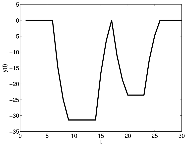
Figure 2: The true output of the FIR model identified in Section VIII-A.

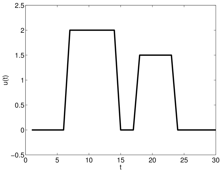
Figure 3: The true input of the FIR model identified in Section VIII-A.

To recover $\{u(t)\}_{t=1}^{30}$ and ${\bf b}$ we use BIL. $\epsilon$ was set to $0$ and $\lambda$ was increased until the first singular value was significantly larger than the second singular value. $\lambda=10^{4}$ gave a first singular value of 64.3 and a second singular value of $9.8\times 10^{-6}$. The estimated input can for this $\lambda$ not be distinguished from the true and the estimate for ${\bf b}$ is equal to the true ${\bf b}$ up the to the numerical precision of the solver after rescaling.

On this simple example, a method that first estimates the input and then the FIR coefficients (for instance [2, 17, 27]) works pretty well. In particular, the naïve approach of first estimating a piecewise input by fitting a piecewise constant signal to the output measurements (use e.g., [22, 29]) and secondly estimate the FIR coefficients gave an as good result as BIL.

VIII-B Identifying an ARX Model From Noisy Data

In this example we use the same input as in the previous example but modify the system to be

$$z(t)= 0.2z(t-1)-4.9594u(t-1)$$

$$+ 6.1774u(t-2)+3.3930u(t-3).$$ (29)

We also assume that there is a uniform measurement noise between $-2$ and $2$ added to the output,

$$y(t)=z(t)+e(t),\quad e(t)\sim U(-2,2).$$ (30)

Given $\{y(t)\}_{t=1}^{30}$ we now aim to find a model of the form

$$z(t)=a_{1}z(t-1)+b_{1}u(t-1)+b_{2}u(t-2)+b_{3}u(t-3),$$ (31)

and a piecewise constant input $\{u(t)\}_{t=1}^{30}$. The given output sequence $\{y(t)\}_{t=1}^{30}$ is shown in Figure 4.

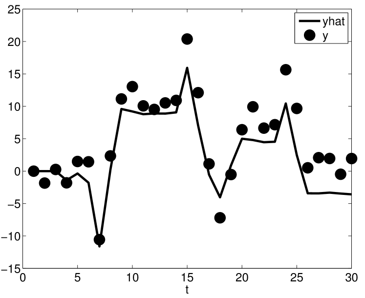
Figure 4: The output measurements $\{y(t)\}_{t=1}^{30}$ given as filled circles and the estimated simulated output obtained by feeding the estimated ARX model with the estimated inputs depicted using solid line.

If we apply BIL with $\lambda=10^{7}$ and $\epsilon=2$ the input shown with solid line in Figure 5 is found. The input associated with the second largest singular value is also shown (gray thin line). The two largest singular values were 43 and 15. Figure 5 also shows the true input with dashed line. Figure 4 shows the output generated by driving the estimated ARX model with the input estimate (both corresponding to the largest singular value of ${\bf X}$).

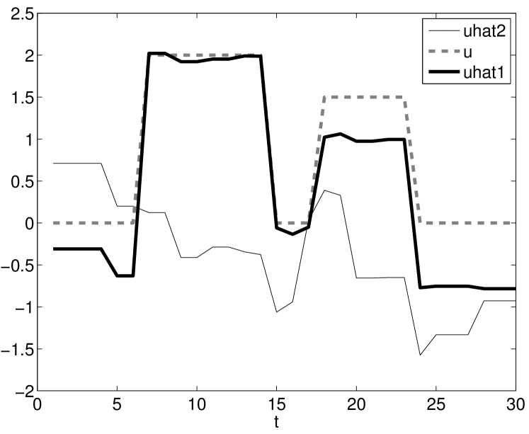
Figure 5: The true input shown using dashed line, the estimate of the input associated with the first singular value of ${\bf X}$ with solid and the estimate associated with the second largest singular value shown with thin gray line.

As in Lasso [33] and my other $\ell_{1}$-regularization problems, it is useful with a refinement step to remove bias. Simply set $\lambda=0$ in BIL and add the constraint

$$\Delta{\bf u}(i)=0\quad\text{ if }\quad|\Delta{\bf u}^{*}(i)|\leq\gamma,\quad i=1,\dots,N-1,$$ (32)

where $\Delta{\bf u}^{*}$ is the previous estimate of $\Delta{\bf u}$ and $\gamma\geq 0$. If we chose $\gamma=0.5$ the input shown in Figure 6 is the result.

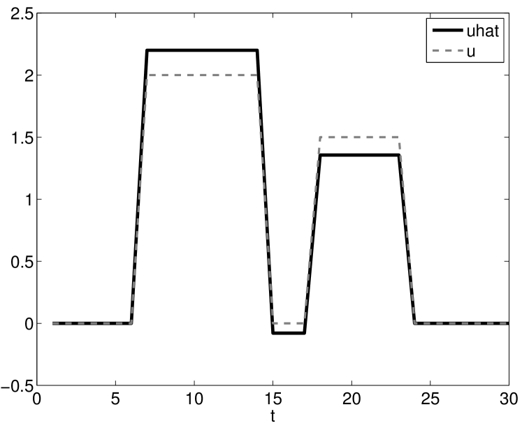
Figure 6: The true input shown with dashed line and the final estimate of the input, after the refinement step, shown with solid line.

The corresponding output obtained by driving the estimated ARX model with the estimated input (both corresponding to the largest singular value of ${\bf X}$ after the refinement step) is given in Figure 7. The two first singular values were now 44 and 5. The estimate for $a$ was 0.2 and $\hat{b}_{1}=-4.5594$, $\hat{b}_{2}=5.7741$, and $\hat{b}_{3}=4.0817$.

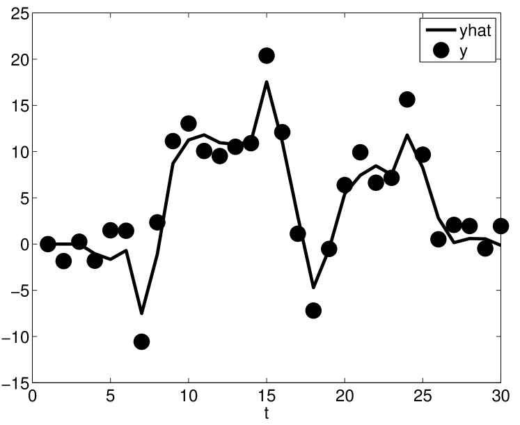
Figure 7: The generated output obtained by feeding the estimated refined ARX model with the refined output estimates shown with solid line. The measured noisy outputs shown with solid circles.

On this more challenging example, the naïve method of first estimating a piecewise input and secondly estimate the ARX coefficients did not give a satisfying result. Figure 8 shows the result of fitting a piecewise constant signal to the outputs and Figure 9 shows compares the true input with the estimated input for the naïve method.

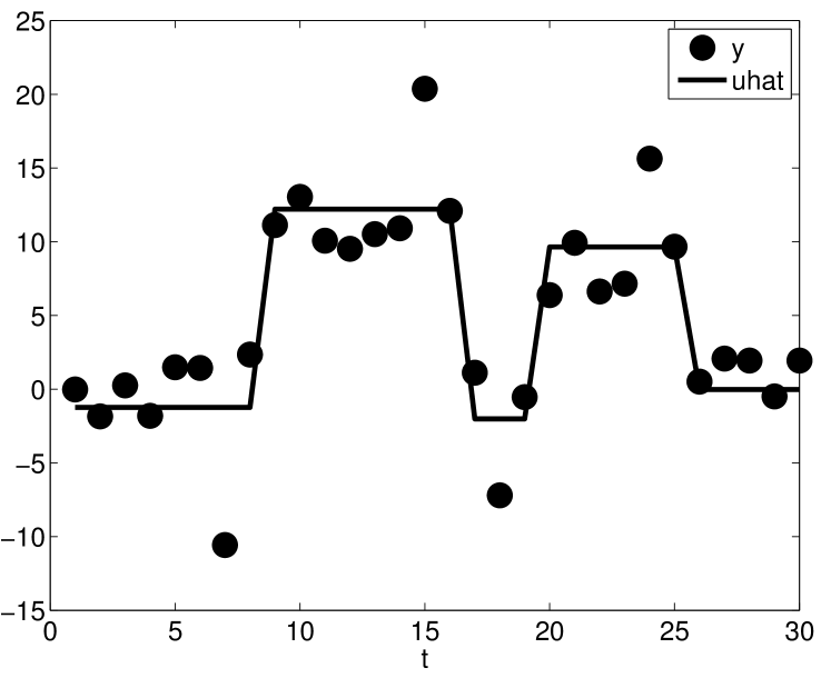
Figure 8: A piecewise constant signal fitted to the measured output.

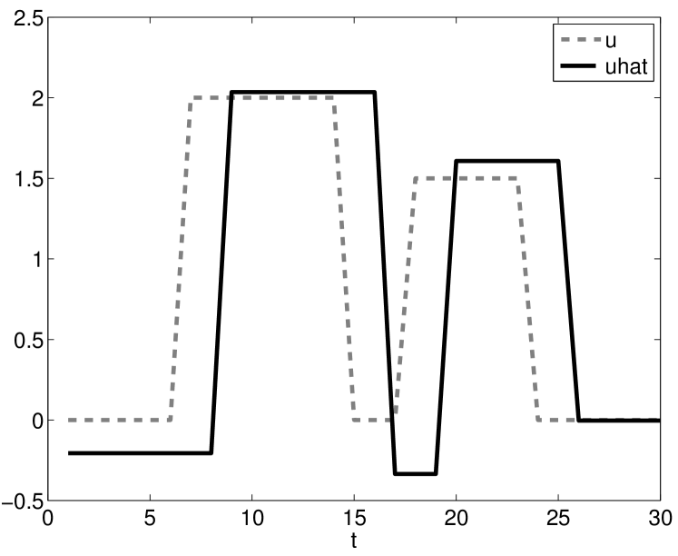
Figure 9: The true input (dashed line) and the estimated input (solid line) by the naïve method.

VIII-C A Real Data Example

This example is motivated by energy disaggregation. The problem of disaggregation refers to the problem of decomposing an aggregated signal into its sources. As an example, the aggregated signal could be the total energy consumed by a house. The sources would then be the energy consumed by different appliances, e.g., the toaster, HVAC, dishwasher etc. In [14], we present a disaggregation algorithm which utilizes models for individual appliances. To model different appliances, the power of individual appliances was measured as they were turned on and off. Figures 10 and 11 show the measured power of a toaster as it was turned on at two different times. To estimate a model for the toaster, we need to estimate both the input and the model at the same time. In addition, we do not want to assume that the input is binary since many appliances have settings that may have changed from one time to the next, e.g., the temperature setting of a toaster etc. We make the assumption that a change in e.g., the temperature of the toaster can be modeled by different input amplitudes. It is therefore more natural to assume that the input is piecewise constant rather than binary.

We chose to use $n_{a}=n_{b}=8$, $n_{k}=0$ $\epsilon=0.04$ and $\lambda=10^{8}$. We subtracted the total mean of both power measurements and sought two input sequences and a set of parameters that well approximate the two power measurement sequences. This resulted in the input estimates shown in Figures 12 and 13.

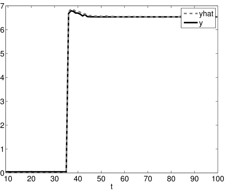
Figure 10: Measured and estimated power consumption of a toaster.

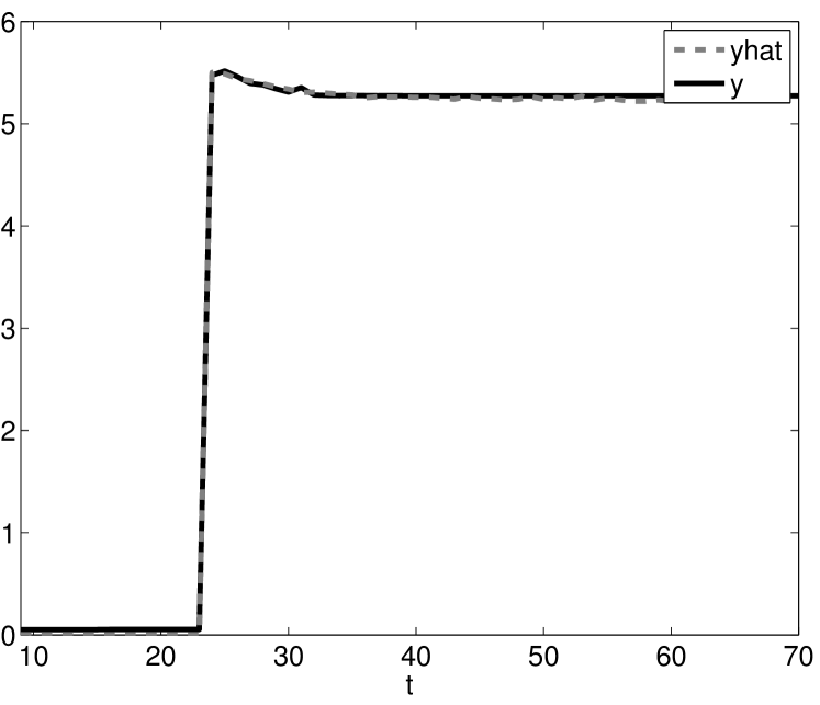
Figure 11: Measured and estimated power consumption of a toaster.

The ARX parameter were computed to:

$${\bf a}=\begin{bmatrix}0.0191\\ 0.0004\\ -0.0006\\ 0.0098\\ 0.0053\\ 0.0065\\ 0.0231\\ -0.0135\end{bmatrix},\quad{\bf b}=\begin{bmatrix}4.6219\\ -0.0527\\ -0.0527\\ -0.0527\\ -0.0567\\ -0.0567\\ -0.0567\\ -0.0683\end{bmatrix}.$$ (33)

Simulating the model provides the power estimates also shown in Figures 10 and 11. The two largest eigenvalues were 32 and 0.07. The found solution is hence very closet to being a rank 1 matrix.

Given aggregated power measurements, we can now use the model of the toaster and seek the a piecewise constant signal representing the toaster being turned on and off. Since it is the power consumption of different devices that are of interest in disaggregation, it is not a problem that we can not identify the inputs or the ARX parameters more than up to a multiplicative constant.

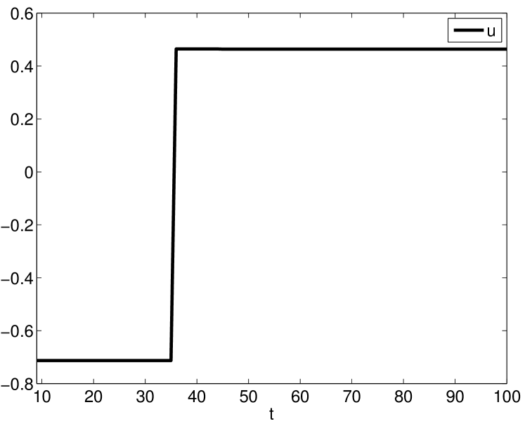
Figure 12: Estimated piecewise constant input to the toaster power measurements seen in Figure 10.

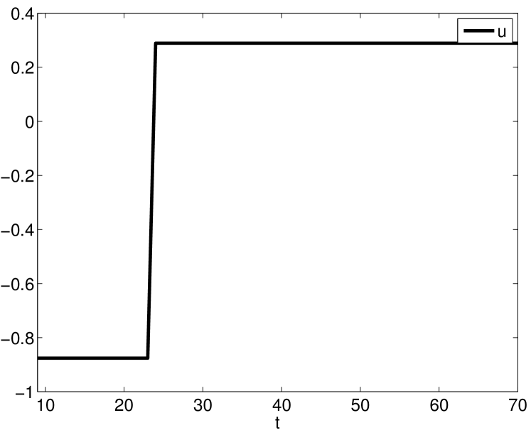
Figure 13: Estimated piecewise constant input to the toaster power measurements seen in Figure 11.

IX Conclusion

This paper presented a novel framework for BSI of ARX model with piecewise constant inputs. The framework uses the fact that the problem can be rewritten as a rank minimization problem. A convex relaxation is presented to approximate the sought ARX parameters and the unknown inputs.

References

- [1] K. Abed-Meraim, J.-F. Cardoso, A.Y. Gorokhov, P. Loubaton, and E. Moulines. On subspace methods for blind identification of single-input multiple-output FIR systems. IEEE Transactions on Signal Processing, 45(1):42–55, Jan.
- [2] K. Abed-Meraim, W. Qiu, and Y. Hua. Blind system identification. Proceedings of the IEEE, 85(8):1310–1322, 1997.
- [3] A. Ahmed, B. Recht, and J. Romberg. Blind deconvolution using convex programming. CoRR, abs/1211.5608, 2012.
- [4] R. Berinde, A. Gilbert, P. Indyk, H. Karloff, and M. Strauss. Combining geometry and combinatorics: A unified approach to sparse signal recovery. In Communication, Control, and Computing, 2008 46th Annual Allerton Conference on, pages 798–805, September 2008.
- [5] D. P. Bertsekas and J. N. Tsitsiklis. Parallel and Distributed Computation: Numerical Methods. Athena Scientific, 1997.
- [6] S. Boyd, N. Parikh, E. Chu, B. Peleato, and J. Eckstein. Distributed optimization and statistical learning via the alternating direction method of multipliers. Foundations and Trends in Machine Learning, 2011.
- [7] A. Bruckstein, D. Donoho, and M. Elad. From sparse solutions of systems of equations to sparse modeling of signals and images. SIAM Review, 51(1):34–81, 2009.
- [8] E. Candès. The restricted isometry property and its implications for compressed sensing. Comptes Rendus Mathematique, 346(9–10):589–592, 2008.
- [9] E. Candès, J. Romberg, and T. Tao. Robust uncertainty principles: Exact signal reconstruction from highly incomplete frequency information. IEEE Transactions on Information Theory, 52:489–509, February 2006.
- [10] E. Candès, T. Strohmer, and V. Voroninski. PhaseLift: Exact and stable signal recovery from magnitude measurements via convex programming. Technical Report arXiv:1109.4499, Stanford University, September 2011.
- [11] E. J. Candès and Y. Plan. Tight oracle bounds for low-rank matrix recovery from a minimal number of random measurements. CoRR, abs/1001.0339, 2010.
- [12] J. N. Caron. Efficient blind deconvolution of audio-frequency signal. Journal of the Acoustical Society of America, 116(1):373–378, 2004.
- [13] A. Chai, M. Moscoso, and G. Papanicolaou. Array imaging using intensity-only measurements. Technical report, Stanford University, 2010.
- [14] R. Dong, L. Ratliff, H. Ohlsson, and S. S. Shankar. A dynamical systems approach to energy disaggregation. In Proceedings of the 52th IEEE Conference on Decision and Control, Florence, Italy, December 2013. Submitted to.
- [15] D. Donoho. Compressed sensing. IEEE Transactions on Information Theory, 52(4):1289–1306, April 2006.
- [16] M. Fazel, H. Hindi, and S. P. Boyd. A rank minimization heuristic with application to minimum order system approximation. In Proceedings of the 2001 American Control Conference, pages 4734–4739, 2001.
- [17] D. Gesbert, P. Duhamel, and S. Mayrargue. On-line blind multichannel equalization based on mutually referenced filters. IEEE Transactions on Signal Processing, 45(9):2307–2317, 1997.
- [18] M. X. Goemans and D. P. Williamson. Improved approximation algorithms for maximum cut and satisfiability problems using semidefinite programming. J. ACM, 42(6):1115–1145, November 1995.
- [19] M. Grant and S. Boyd. Graph implementations for nonsmooth convex programs. In V. D. Blondel, S. Boyd, and H. Kimura, editors, Recent Advances in Learning and Control, Lecture Notes in Control and Information Sciences, pages 95–110. Springer-Verlag, 2008. http://stanford.edu/~boyd/graph_dcp.html.
- [20] M. Grant and S. Boyd. CVX: Matlab software for disciplined convex programming, version 1.21. http://cvxr.com/cvx, August 2010.
- [21] Y. Hua. Fast maximum likelihood for blind identification of multiple FIR channels. IEEE Transactions on Signal Processing, 44(3):661–672, 1996.
- [22] S.-J. Kim, K. Koh, S. Boyd, and D. Gorinevsky. trend filtering. SIAM Review, 51(2):339–360, 2009.
- [23] T.-H. Li. Blind deconvolution of discrete-valued signals. In Conference Record of The Twenty-Seventh Asilomar Conference on Signals, Systems and Computers, pages 1240–1244. IEEE, 1993.
- [24] L. Ljung. System Identification — Theory for the User. Prentice-Hall, Upper Saddle River, N.J., 2nd edition, 1999.
- [25] J. Löfberg. YALMIP: A toolbox for modeling and optimization in MATLAB. In Proceedings of the CACSD Conference, Taipei, Taiwan, 2004.
- [26] L. Lovász and A. Schrijver. Cones of matrices and set-functions and 0-1 optimization. SIAM Journal on Optimization, 1:166–190, 1991.
- [27] J. I. Makhoul. Linear prediction: A tutorial review. Proceedings of the IEEE, 63(4):561–580, April 1975.
- [28] Y. Nesterov. Semidefinite relaxation and nonconvex quadratic optimization. Optimization Methods & Software, 9:141–160, 1998.
- [29] H. Ohlsson, L. Ljung, and S. Boyd. Segmentation of ARX-models using sum-of-norms regularization. Automatica, 46(6):1107–1111, 2010.
- [30] H. Ohlsson, A. Y. Yang, R. Dong, M. Verhaegen, and S. S. Sastry. Quadratic basis pursuit. CoRR, abs/1301.7002, 2013.
- [31] N.Z. Shor. Quadratic optimization problems. Soviet Journal of Computer and Systems Sciences, 25:1–11, 1987.
- [32] S. Talwar, M. Viberg, and A. Paulraj. Blind estimation of multiple co-channel digital signals using an antenna array. IEEE Signal Processing Letters, 1(2):29–31, 1994.
- [33] R. Tibsharani. Regression shrinkage and selection via the lasso. Journal of Royal Statistical Society B (Methodological), 58(1):267–288, 1996.