Evolution of Galaxies and their Environments
at z = 0.1 to 3 in COSMOS

Abstract

Large-scale structures (LSS) out to z $<3.0$ are measured in the Cosmic Evolution Survey (COSMOS) using extremely accurate photometric redshifts (photoz). The Ks-band selected sample (from Ultra-Vista) is comprised of 155,954 galaxies. Two techniques – adaptive smoothing and Voronoi tessellation – are used to estimate the environmental densities within 127 redshift slices. Approximately 250 statistically significant overdense structures are identified out to z $=3.0$ with shapes varying from elongated filamentary structures to more circularly symmetric concentrations. We also compare the densities derived for COSMOS with those based on semi-analytic predictions for a $\Lambda$CDM simulation and find excellent overall agreement between the mean densities as a function of redshift and the range of densities. The galaxy properties (stellar mass, spectral energy distributions (SEDs) and star formation rates (SFRs)) are strongly correlated with environmental density and redshift, particularly at z $<1.0-1.2$. Classifying the spectral type of each galaxy using the rest-frame b-i color (from the photoz SED fitting), we find a strong correlation of early type galaxies (E-Sa) with high density environments, while the degree of environmental segregation varies systematically with redshift out to z $\sim 1.3$. In the highest density regions, 80% of the galaxies are early types at z=0.2 compared to only 20% at z = 1.5. The SFRs and the star formation timescales exhibit clear environmental correlations. At z $>0.8$, the star formation rate density (SFRD) is uniformly distributed over all environmental density percentiles, while at lower redshifts the dominant contribution is shifted to galaxies in lower density environments.

1 Introduction

The cosmic evolution of galaxies and dark matter is strongly linked through both the environmental influences and feedback due to starbursts and AGN. Peng et al. (2010) have recently shown that the quenching of star formation (SF) activity in low redshift SDSS galaxies is clearly separable into galaxy-mass and environmental-density dependent effects. A major motivation for the Cosmic Evolution Survey (COSMOS) was to provide a sufficiently large area, to probe the expected range of environments (large-scale structure – LSS) with high sensitivity to detect large samples of objects at high redshifts, and to minimize the effects of cosmic variance. The COSMOS 2 deg² survey samples scales of LSS out to $\sim$ 50 – 100 Mpc and detects approximately two million galaxies at z $=0.1-5$ at I $<26.5$ mag(AB). Initial identifications of LSS galaxy clusters in COSMOS were compared with the total mass densities determined from weak lensing tomography and hot X-ray emitting gas in the virialized clusters/groups of galaxies at z $<1.1$ (Scoville et al., 2007b; Massey et al., 2007; Finoguenov et al., 2007); here we extend this investigation to higher z and lower density LSS using deeper photometry and high accuracy photometric redshifts.

The identification of LSS from the observed surface-density of galaxies requires separation of galaxies at different distances along the line of sight, otherwise, the superposition of LSS at different redshifts would preclude a mapping of the structure morphology and the LSS overdensities would be diluted by foreground and background galaxies. Ideally, redshift (or distance discrimination) precision is desired at the level of the internal velocity dispersions of the structures. For LSS mapping, line-of-sight discrimination is usually accomplished using: 1) color selection (e.g. using broadband colors to select red sequence galaxies, Gladders & Yee, 2005); 2) spectroscopic redshifts (in COSMOS e.g., Kovač et al., 2010; Peng et al., 2010) and 3) photometric redshifts derived from fitting the broadband spectral energy distributions (SEDs) of the galaxies (van de Weygaert, 1994; Postman et al., 1996; Schuecker & Boehringer, 1998; Marinoni et al., 2002). Color selection clearly biases any correlation between environment and galaxy SED or morphological type (Dressler et al., 1997; Smith et al., 2005) since the resulting LSS are a priori based on a particular SED type (e.g. early type galaxies). In addition, the red early-type galaxies must become rarer at early epochs, simply due to the short cosmic age, and identification of clustering using the red sequence is bound to become problematic at higher redshifts. Spectroscopic redshifts are of course most desirable and have been used extensively in low z studies with relatively bright galaxies (e.g. SDSS); however, they are not presently feasible for the samples of hundreds of thousands of high redshift galaxies going fainter than $I_{AB}=24$ mag and galaxies lacking strong emission lines. Spectroscopy of such faint galaxies requires the largest telescopes and integration times of a few hours (Le Fèvre et al., 2005; Gerke et al., 2005; Meneux et al., 2006; Cooper et al., 2006; Coil et al., 2006; Lilly et al., 2007).

In this paper, we identify LSS in the 2 square degree COSMOS field using the most recent COSMOS photometric redshifts (Ilbert et al., 2009, 2013) to analyze the galaxy surface densities in redshift slices out to z = 3.0, covering cosmic ages from 2.1 to 12 Gyr. These photometric redshifts are extremely accurate (see §2) since they are based on deep 30-band UV-IR photometry and they cover all galaxy spectral types. The galaxy sample used for this work and the associated stellar mass limits are discussed in §2 and a similar sample is generated from a $\Lambda$CDM simulation of size 1/64 of Millennium (§2.3). We use two independent techniques: adaptive smoothing (Scoville et al., 2007b) and 2-d Voronoi tessellation (Ebeling & Wiedenmann, 1993) to measure the local density associated with each galaxy, and to map and visualize coherent LSS in COSMOS (§3). Maps of the LSS are presented in §4. The derived densities are compared with predictions from the simulation (§5). We analyze the evolution of the galaxy population with redshift and environmental density in §6 and a simplified schematic model for the evolution processes is presented in §6.5.

Adopted cosmological parameters, used throughout, are: H₀ = 70 km s^-1 Mpc^-1, $\Omega_{M}$ = 0.3 and $\Omega_{\Lambda}$ = 0.7. The AB magnitude system is used throughout. For computing stellar masses and star formation rates (SFRs), we adopt a Chabrier IMF; for the Salpeter IMF, both the mass and SFR estimates should be increased by a factor of 1.78.

Figure 1: Comparison of photometric and spectroscopic redshifts for a sample of 12,482 galaxies down to $I_{AB}\sim 24.5$ mag in COSMOS (figure taken directly from Ilbert et al., 2013). For this sample, the $\sigma_{z}/(1+z)$ = 0.9% and the catastrophic failure rate is 2%. The dotted lines indicate the 2 $\sigma$ dispersions. The COSMOS photometric redshifts are from Ilbert et al. (2013) and the spectroscopic redshifts are from: the zCOSMOS VIMOS bright (black squares) and faint (blue x’s) surveys (Lilly et al., 2007), the Keck DEIMOS survey (green x’s, Capak et al. 2013 in preparation), the FORS2 survey (brown triangles, Comparat et al. 2013 in preparation), the FMOS survey (cyan stars,  Silverman et al.2013 in preparation), the MOIRCS survey (red circles, Onodera et al. (2012)), and the WFC3 grism survey (red triangles, Krogager et al. 2013 in preparation). Only galaxies with reliable (at least 2 spectral lines) spectroscopic redshifts are used here.

2 Photometric Redshifts and Sample Selection

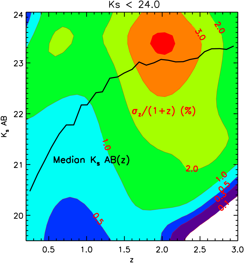
Figure 2: The accuracy ($\sigma_{z}/(1+z)$ in %) for the photometric redshifts is shown as a function of observed Ks-band magnitude and redshift. These uncertainty estimates were derived from the dispersion in the photoz probability density distributions (PDF) as discussed in the text. For bright galaxies at z $<1.2$, $\sigma_{z}/(1+z)<$ 1% but degrades by a factor of two at higher z and for fainter galaxies. Also shown is the median magnitude, Ks_AB, for galaxies in our sample – the widths of the redshift slices is chosen to approximately follow the FWHM (=2$\sigma_{z}$) of the median galaxy at each z.

The COSMOS photometric catalog is derived from deep ground and space-based imaging in 37 broad and intermediate-width bands. This includes HST-ACS F814W (Scoville et al., 2007a), Suprime-Cam on Subaru (Taniguchi et al., 2007) and CFHT-MagaCam/WIRCam (McCracken et al., 2010); near infrared imaging (Y, J, H & K_s) from NOAO-4m, UH88, UKIRT (Capak et al., 2007; McCracken et al., 2010), Ultra-Vista (McCracken et al., 2012); Spitzer IRAC 3.6-8.5$\mu$m (Sanders et al., 2007) and Galex NUV & FUV (Zamojski et al., 2007). Typical sensitivities (5$\sigma$ in a 3^′′aperture) are 26-27 mag (AB) in the optical and 25 mag (AB) in the infrared (Capak, 2009; McCracken et al., 2012). The original COSMOS photometric catalogs were based on primary source detections in the Subaru and CFHT i-band imaging. 2.1 million objects are included at I${}_{AB}<26.5$ mag (Capak, 2009). The new catalog we make use of here is based on primary source detection in the Ultra-Vista Ks band and this provides significantly better completeness at $z>1$, especially for red or passive galaxies.

The COSMOS photometric redshift (photoz) catalog using primary source selection in Ks band is described in detail in Ilbert et al. (2013). For these most recent photometric redshifts the 30 broad, intermediate and narrow bands include : u^∗, BJ, VJ, r⁺, i⁺, z⁺, IA484, IA527, IA624, IA679, IA738, IA767, IA427, IA464, IA505, IA574, IA709, IA827, NB711, NB816, the four Spitzer IRAC bands and four UltraVISTA bands (Y, J, H, Ks). Photoz were derived for 218,000 galaxies with Ks (AB)$<24$ mag using a $\chi^{2}$ template fitting procedure (Le Phare : Arnouts et al., 2002; Ilbert et al., 2006). The fitting presumes 31 basic spectral energy distributions (SEDs) with dust extinctions varying from A_V = 0 to 1.5 mag with Calzetti et al. (2000) and Prevot et al. (1984) extinction laws. Emission lines are included in the photoz fitting.

Spectroscopic redshifts in COSMOS have been obtained from the VLT-VIMOS zCOSMOS survey (Lilly et al., 2007) for approximately 20,000 galaxies (I${}_{AB}\leq 24.5$ mag) and Keck-DEIMOS (Capak, 2013) for approximately 3400 galaxies (I${}_{AB}\leq 25$ mag). The offsets between the photometric and spectroscopic redshifts for 12,482 galaxies with high reliability spectroscopic redshifts at z = 0.05 to 4 down to I${}_{AB}\leq 24.5$ mag yield $\sigma_{z}/(1+z)\simeq$ 0.9% with a catastrophic ($>2\sigma$) failure rate typically only 2% as shown in Fig. 1 (Ilbert et al., 2013).

2.1 Sample Selection

For this study, we adopt selection criteria requiring that the galaxies be detected in the near infrared band (K_s and in most cases they are detected in IRAC1-3.6$\mu$m) – in order to provide more reliable mass estimates from the long wavelength continuum. We exclude objects classified as stellar or AGN-dominated as indicated by their measured size in the HST-ACS images or an X-ray detection. We impose the following selection criteria on the Ultra-Vista Ks selected photoz redshift catalog :

$$z=0.15-3.0$$ (1a)

$$K_{s}(AB)\leq 24~{}mag$$ (1b)

$$M_{*}\geq 10^{9}\mbox{$M_{\odot}$}~{}$$ (1c)

$$149.4{{}^{\circ}}<\alpha_{2000}<150.8{{}^{\circ}}~{}~{}~{}\rm{and}~{}~{}~{}1.5{{}^{\circ}}<\delta_{2000}<2.9{{}^{\circ}}.$$ (1d)

The stellar mass (see §2.2) selection criteria was imposed so that the LSS would be mapped using reasonably massive galaxies; it has impact only at z $<$ 0.5 since such low mass galaxies are not detected at the higher redshifts. The last selection by position, was used to provide an approximately square area for imaging LSS, and to minimize the effects of the irregular Ultra-Vista coverage at the field edges. These four combined selection criteria yield a sample of 155,954 galaxies. [All areas masked for proximity to a bright star were also excluded, as shown in Fig. 29.] A principal goal of this study is to explore the correlation of galaxy properties with environment and redshift. Thus, it is important to recognize that we have avoided selection based on a specific type of galaxy, i.e. using colors to select red sequence galaxies.

The above selection criteria were arrived at as a compromise between two goals: 1) maintaining high accuracy in redshifts to enable narrow redshift slices for delineating the LSS and 2) providing large samples of galaxies in each slice so that the LSS can be traced to lower densities. Trials with the simulation mock catalogs (see §2.3) indicated that redshift slice widths of $\Delta z\sim 1-2$% at z = 1 and $\sim$ 5-10% at z = 2 are adequate for detecting the LSS without excessive contamination or dilution of the LSS.

The spectroscopic/ photometric redshift comparison shown in Fig. 1 is limited to a sample of only 12,482 galaxies (mostly brighter objects). To extend our understanding of the photoz uncertainties, we used the probability distribution function (PDF) from the photometric redshift solutions for a more general assessment of the redshift accuracies as a function of both redshift and magnitude. As discussed in Ilbert et al. (2009), the width of the highest peak in the PDF agrees well with that of the specz-photoz comparison at redshifts and magnitudes where there are sufficient spectroscopic redshifts for a comparison (see Fig. 9; Ilbert et al., 2009). Fig. 2 shows $\sigma_{z}/(1+z)$ as a function of redshift and galaxy magnitude from the Ks-selected photoz catalog. For sources with spectroscopic redshifts, the PDF yields uncertainty estimates in good agreement with the dispersions between the spectroscopic and photometric redshifts shown in Fig. 1 (Ilbert et al., 2013).

Fig. 2 shows that at Ks (AB)$<22.5$ and low z, $\sigma_{z}/(1+z)<0.01$ but the accuracy degrades significantly at fainter magnitudes and above $z\sim 1.1$. The black line in Fig. 2 indicates the median observed Ks-magnitude of galaxies in our sample as a function of redshift. At z $=1$, a redshift slice of width $\Delta z=0.02$ ($\sim 2\sigma_{z}$) is appropriate while at z $=2$ the width should increase to $\sim 0.2$. In fact, these variable width bins in redshift result in fairly similar spans in lookback time ($\Delta t_{LB}=0.17-0.42$ Gyr).

2.2 Galaxy Classification, Stellar Mass and SFR

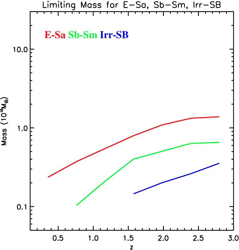
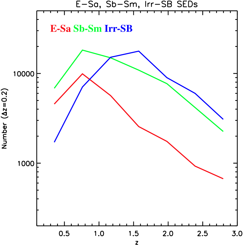
Figure 3: For the sample selection with K${}_{s}<24$, yielding 155,954 galaxies, the stellar mass limits for early, spiral and starburst galaxies are shown as a function of redshift together with the number counts of each type in bins of width $\Delta z=0.2$. The lower mass limit for galaxy selection was $10^{9}$$M_{\odot}$ . The small breaks in these curves are a result of the SED features redshifting through the COSMOS photometric bands which have varying sensitivities. The actual sample selection is given by the joint criteria given in Eq. 1d. The gradual drop in the counts of red galaxies above z = 1.5 (right panel) is due to both their decreased numbers at high z and the fact that the red galaxies have lower fluxes rest frame blue which is redshifted to the Ks selection band. The decreases in total number counts at $z<0.5$ are due simply to the decreased cosmic volume. Extensive discussion of the mass completeness is provided in Ilbert et al. (2013).

In the most recent COSMOS photoz catalog which is used here, stellar masses and SFRs were derived from fitting the template SEDs to BC03 models (Bruzual & Charlot, 1993) as discussed in Ilbert et al. (2013). These models assume a Chabrier stellar initial mass function (IMF, Chabrier (2003)). The SFRs were estimated from both the rest frame UV continuum and the Spitzer 24$\mu$m flux (for galaxies with 24$\mu$m detections). In cases where both IR and UV SFRs were available, we used a SFR given by the extincted UV continuum plus the IR SFR. For the IR-based SFRs, the 24$\mu$m fluxes were converted to total L_IR using the procedures of Lee et al. (2010) and using $SFR$($M_{\odot}$ /yr)$=1.14\times 10^{-10}$(L_IR/$L_{\odot}$ ). For galaxies lacking a 24$\mu$m detection, the SFR was estimated from the extinction-corrected UV continuum derived from the photoz SED fitting, using the relations given in Kennicutt (1998) and Schiminovich et al. (2005) scaled to the Chabrier IMF, i.e. $SFR=1.0\times 10^{-28}L_{\nu}(NUV)$ (cgs). In order to study the impact of galaxy SED on our results, we assigned a type to each of them according to their rest-frame B-i color (including reddening), using the types : ’SB1’, ’Im’, ’SB2’, ’Sd’, ’Sc’, ’Sb’, ’Sa’, ’S0’ and ’E’, respectively (similar to the b-i color classes of Arnouts et al., 2005, but shifted slightly to account for the different COSMOS filter bandpasses). For the analysis here we define three broad classes with b-i color: $>0.84$ (E-Sa), 0.45 - 0.84 (Sab-Sd) and $<0.45$ (IRR/SB).

Although color selection was not used for the sample, the resultant mass limits differ for the red and blue galaxies as a function of redshift. Figure 3 shows the stellar mass limits for three characteristic SED types (early, spiral and starburst) resulting from the photometric selection criteria in Eq. 1d. To compute the limiting mass curves shown in Fig. 3, we derived the mean mass-to-light ratios (using the observed magnitudes in the Ks filter) for all the galaxies of each spectral class as a function of redshift, and then scaled this ratio by the limiting magnitude (24 AB). (These limits correspond to $\sim 75$% completeness.) The number counts of the three basic SED types with the combined selection criteria are also shown. The mass limits clearly depend on the SED of the galaxy, but having a catalog with primary source selection in Ks (rather than optical bands) greatly reduces the bias against early types (Ilbert et al., 2013). The starburst galaxies are relatively bright at short wavelength, and therefore easier to detect in the observed optical at high redshift, since their UV continua will be redshifted to optical bands. In contrast, the early type red galaxies become much more difficult to detect at high redshift (i.e. a higher stellar mass is required) since they have relatively weak restframe UV continua. This difficulty is alleviated to some extent by the fact that at $z=1-2$ the mass function of passive (red) galaxies appears to have decreased numbers of low mass systems ($<10^{10.8}$$M_{\odot}$ ) compared to higher masses (Ilbert et al., 2010, 2013); thus the lower mass red galaxies are intrinsically rare above z = 1. The percentage of passive, intrinsically red galaxies, is of course also much lower at z $>1$ (Ilbert et al., 2013).

The Ks band photometric selection results in mass detection limits: 0.3, 0.6, 0.8 and 1.5 $\times 10^{10}$$M_{\odot}$ at z = 0.5, 1, 1.5 and 2.5 for the E-Sa SED types. For the Irr-SB SED types, the equivalent limits are: $<$0.08, 0.1, 0.12 and 0.2 $\times 10^{10}$$M_{\odot}$ at z = 0.5, 1, 1.5 and 2.5. [The explicit mass selection in Eq. 1d removes all galaxies with mass below $10^{9}$$M_{\odot}$ .] At z = 0.5 to 2 , the knee in the galaxy stellar mass function drops from $logM_{*}=10.9$ to 10.6 $M_{\odot}$ , i.e. from 8 to 4$\times 10^{10}$ $M_{\odot}$ (Ilbert et al., 2013) for quiescent galaxies. For the blue galaxy SEDs, our selection reaches more than an order of magnitude below these M_∗ values, even at the highest redshifts. For the red SEDs, the mass limit reaches $<0.2$ M_∗ all the way to z $\sim$3.

2.3 $\Lambda$CDM Simulation

One of the goals of this study is a comparison of the observed evolution in the COSMOS LSS with current theoretical models. For this, we make use of mock simulation catalogs generated for an area and volume equivalent to the COSMOS survey. The mock catalogs are based on $\Lambda CDM$ simulations which start at z = 127 evolved down to z = 0 (Wang et al., 2008). For comparison with the COSMOS data we make use of their WMAP3YC simulation, which adopts cosmological parameters derived from a combination of third-year WMAP data on large scales, and Cosmic Background Imager and extended Very Small Array data on small scales (Spergel et al., 2007) (with $\Omega_{M}=0.226$ and $\Omega_{\Lambda}=0.774$). Their mass and force resolution are the same as used in the Millennium Simulation (Springel et al., 2005), while the volume is smaller by a factor of 64.

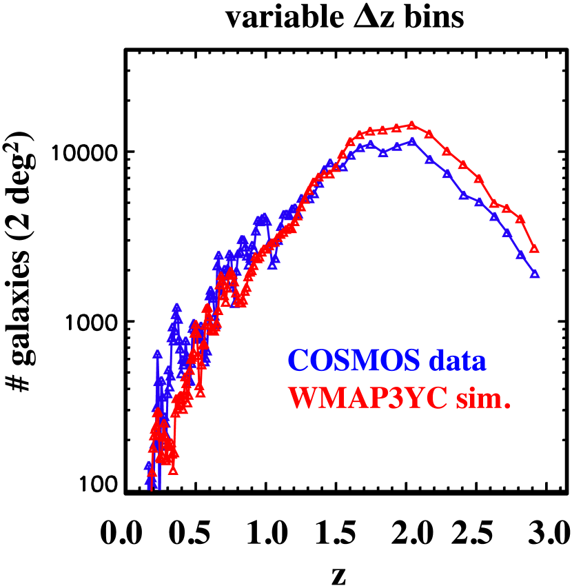
Figure 4: The redshift distributions for COSMOS (blue) and simulation galaxies (red)) are shown for the adopted selection criteria (K${}_{s}<24$ AB mag at z = 0.15 to 3.0). The width $\Delta z$ of the redshift slices varies with redshift to match the photoz accuracy (Fig. 2), i.e. larger width bins at high z. These are the same bin widths used in the LSS mapping, giving 1000 to 10000 galaxies in each redshift slice at z $>$0.5. Note that these bins are spaced by half a bin width so the total number counts are half of the sums obtained from this figure.

The galaxy formation model of De Lucia & Blaizot (2007) was adopted to calculate the galaxy properties. This model has been able to reproduce many aspects of local galaxy populations (e.g. Croton et al., 2006; De Lucia & Blaizot, 2007) and high redshift galaxy properties (Kitzbichler & White, 2007; Guo & White, 2009). For WMAP3, two sets of parameters are found to reproduce the local observational data (see Wang et al., 2008; De Lucia & Blaizot, 2007; Croton et al., 2006; Springel et al., 2005). The simulations track halo dark matter masses, star formation rates (SFRs) and stellar masses.

This simulation was extremely valuable for evaluating the effectiveness of our techniques for identifying LSS in the presence of redshift errors similar to those of the COSMOS photoz, and for analysis of the scaling between the derived 2-d surface densities of galaxies and the 3-d volume density of galaxies, for the range of LSS expected to be present at high redshift.

The mock catalog includes photometric magnitudes in the COSMOS filter passbands from FUV to IRAC1-4 and rest frame absolute magnitudes, with and without dust extinction. Galaxies were selected from the simulation using the same photometric cuts/limits as used for COSMOS (Eq. 1d). Redshifts from the simulations were also scattered with a dispersion identical to those in the COSMOS photometric redshifts, as a function of magnitude and redshift (see Fig. 2). A known problem with the simulation is an overabundance of low stellar mass galaxies (see Fig. 1 in Guo et al., 2011); to alleviate this problem, we imposed a stellar mass limit of $2\times 10^{9}$$M_{\odot}$ (instead of $10^{9}$$M_{\odot}$ ) to yield similar sample sizes to the observed galaxy sample. In each mock catalog, two dust extinction curves (’dust1’ and ’dust2’) were employed to relate the dust extinction to the surface density of HI and the metallicity of the ISM. The major difference between the two dust models is that the ’dust2’ has weaker dependence on redshift (Guo & White, 2009) to better reproduce the observed counts of Lyman break galaxies (Guo & White, 2009). In this paper, we compare observational results with the WMAP3YC model using the magnitudes computed with the ’dust2’ extinction curve.

The redshifts of the galaxies from the simulation were then dispersed with the same uncertainties as for the COSMOS photoz catalog (Fig. 2). The LSS in the simulation was also measured with the same routines used for the COSMOS galaxy sample (§3). Fig. 4 shows a comparison between the redshift distributions of galaxies in the mock and in the COSMOS sample used here. Overall, there is very good correspondence in the two redshift distributions.

3 Galaxy Environmental Densities

The environmental density for each galaxy was derived from the local surface density of galaxies within the same redshift slice (§3.1) based on the high accuracy COSMOS photometric redshifts for the 155,954 galaxies. [We note that Knobel et al. (2009, 2012) provide a catalog of galaxy groups and Kovač et al. (2010) the density field, both based on the zCOSMOS spectroscopic redshifts for 16,500 galaxies.] Two techniques were employed here to map the LSS: adaptive spatial smoothing and Voronoi 2-d tessellation (§3.2).

3.1 Redshift Slices

For mapping LSS it is vital that the binning in redshift be matched to the accuracy of the redshifts, to provide optimum detection of the overdensities associated with LSS. Using redshift bins that are finer than the redshift uncertainties distributes the galaxies from a single structure over multiple redshift slices and thus reduces the signal-to-noise ratios in each slice. Conversely, bins of width larger than the redshift uncertainties will increase the shot noise associated with foreground and background galaxies, relative to the large-scale structure signal, i.e. galaxies from neighboring redshifts are superposed on the LSS at the redshift of interest.

For the adaptive smoothing algorithm discussed in Scoville et al. (2007b), each galaxy is distributed in z according to its photoz PDF (probability density function); for the Voronoi tessellation, each galaxy is placed at the maximum likelihood photometric redshift. (Rather than using the minimum chisq photoz, we use the median of the marginalization of the redshift probability distribution.) If the uncertainties in the galaxy redshifts were a Gaussian distribution, the optimum smoothing or binning in redshift would be a Gaussian of FHWM $\simeq 2\sigma_{z}$ (if there are approximately equal densities of galaxies in LSS, and a uniformly distributed field population). The width of this optimum redshift binning should increase as the number of randomly superposed ’field’ galaxies is decreased. In the following, we adopt redshift bin widths of $\Delta z=2\sigma_{z}$ where $\sigma_{z}/(1+z)$ is shown in Fig. 2 as the line corresponding to the expected uncertainty at the median magnitude of sample galaxies as a function of redshift. The adjacent redshift slices are spaced by half of the width of the slices at each redshift. The result is a total of 127 redshift slices ranging from z $=0.15$ to 3.0 which are analyzed for significant LSS. This results in the bins having galaxy counts as shown in Fig. 4.

3.2 Galaxy Density Measurements

Two techniques are used here to image the LSS environments in the galaxy surface density distribution in the 127 redshift slices : adaptive spatial filtering and Voronoi 2-d tessellation. The former was developed and tested in our previous analysis of COSMOS LSS (see Scoville et al., 2007b); the latter has been used in many earlier investigations of galaxy LSS (van de Weygaert, 1994; Ebeling & Wiedenmann, 1993; Marinoni et al., 2002; Gerke et al., 2005). Both techniques are used here since each has clear advantages and disadvantages and the generally good agreement in the derived density fields provides confidence in the results of both (see Fig. 5). The sample numbers shown in the figures below are less than the total sample of 155,954 galaxies, since galaxies at the edge of the survey area do not have closed Voronoi polygons.

The adaptive smoothing procedure has a clearly specified level of significance, and structures of lower statistical significance are simply not detected. On the other hand, the adaptive filtering which makes use of a variable width Gaussian spatial smoothing function is less appropriate than the Voronoi tessellation for detection of elongated and irregular structures. The latter technique locates the polygon area closest to each galaxy and is therefore not making an assumption of structure shape. For the adaptive smoothing the tests, run on a ’redshift slice’, in which 50% of the galaxies were in modeled overdense concentrations and 50% were randomly distributed, showed extremely good proportionality between the recovered densities and the models, with virtually no spurious features when compared to the input model (see Appendix in Scoville et al. (2007b).

A second difference between these techniques arises from the fact that adaptive smoothing searches a defined range of angular scales, whereas the Voronoi tessellation is unrestricted. For the former, the data is spatially binned in 600$\times$600 pixels (0.2^′) across the 2 deg field and smoothing filters from 1 to 60 pixels (FWHM) are searched for significant overdensity. The filtering width thus corresponds to 0.2^′ to 0.2^∘ , corresponding to comoving scales of 200 kpc to 12 Mpc at z = 1. Thus one anticipates that the Voronoi technique can yield higher densities on scales smaller than 0.2^′ or in elongated structures. The Voronoi technique will also provide a density estimate for all galaxies independent of whether the environmental density is statistically significant. The latter can be an advantage or a disadvantage depending on how the density estimates are to be employed, so we feel it is beneficial to have both density fields.

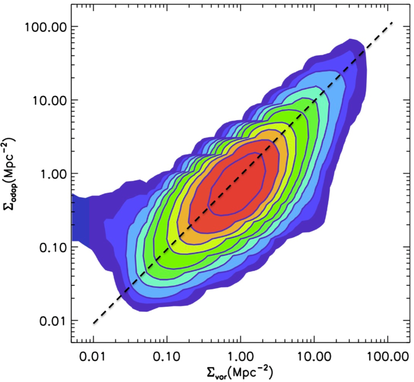
Figure 5: The environmental densities obtained from the adaptive smoothing and Voronoi techniques are compared for the sample of 150,852 galaxies. Contours are at 0.0005, 0.001, 0.002, 0.005, 0.01, 0.02, 0.05, 0.1, 0.2 and 0.5. Over almost 3 orders of magnitude in the surface density, the two techniques give similar results following a line of 1:1 correspondence along the ridge line with the highest number of objects. The deviation seen on the outermost contour on the left side is due to the fact that the adaptive smoothing is designed to detect only statistically significant overdensities in each redshift slice whereas the Voronoi densities are derived everywhere.

Both techniques yield the 2-d surface density of galaxies in each redshift slice rather than the true 3-d volume density of galaxies. Direct determination of the 3-d volume densities would require more precise redshifts and a means of correcting for non-Hubble flow streaming and increased velocity dispersion due to LSS mass concentrations. The accuracy of the redshifts would need to be a factor of $\sim 10$ higher to resolve the cluster velocity dispersions. In the very dense environments, the increased velocity dispersions may actually indicate that the 2-d surface densities provide a more robust measure of the galaxy environment (provided this surface density is mostly dominated by the LSS in the slice with little foreground and background contamination). In general, one expects proportionality between the derived projected 2-d and true 3-d densities as long as the redshift slices are fine enough that there are few galaxies superposed from other redshifts. To test the proportionality, we have run both the adaptive smoothing and Voronoi 2-d tessellation algorithms on the simulation mock catalog. Since the simulation has accurate 3-d positions, we were also able to evaluate the 3-d densities using a 3-d tessellation.We found that for the galaxy densities and redshift uncertainties in our samples, the 2-d projected densities were monotonically related to the true 3-d volume densities with a $\sim 0.67$ power law as expected for linear structures.

3.3 Comparison of Adaptive Smoothing and Voronoi Densities

The adaptive smoothing and Voronoi techniques give estimates for the local surface densities of galaxies which are in reasonable correspondence, given their very different approaches and assumptions (as discussed above in §3.2). Figure 5 shows the distribution of the $\Sigma_{adap}$ versus $\Sigma_{vor}$ for the sample of 150,852 galaxies. This number of galaxies is slightly less than the sample number quoted earlier since the Voronoi polygons are not closed at the outer edges of the field and no area and density estimate is obtained for those galaxies. Over $\sim$3 orders of magnitude in the surface density the two techniques give similar results with the ridge line for the highest number of objects tilted somewhat, relative to the shown 45 degree equality line. The tilt offset is due to the fact that the adaptive smoothing algorithm only recovers densities at a smoothing scale length such that the density is statistically significant, whereas the Voronoi densities do not have this restriction. Deviations can also be seen in the outer 4 contours at level 1/256 of the peak : these are due to the ability of the Voronoi to go to effectively higher resolution at higher densities. The maximum resolution in the adaptive smoothing is set at 1/600 of the field or $\sim$10.8^′′).

In the following, we use the densities derived from the Voronoi tessellation for correlating galaxy properties with environmental density. The tessellation provides an estimate of the environment of all galaxies even if these are not significantly overdense. On the other hand, the adaptive smoothing is more appropriate for the identification of statistically significant large scale structures if that is required (although not the subject of the work here).

The environmental density estimates in the COSMOS field as derived here are available for download from the IPAC/IRSA COSMOS archive at http://irsa.ipac.caltech.edu/data/COSMOS/.

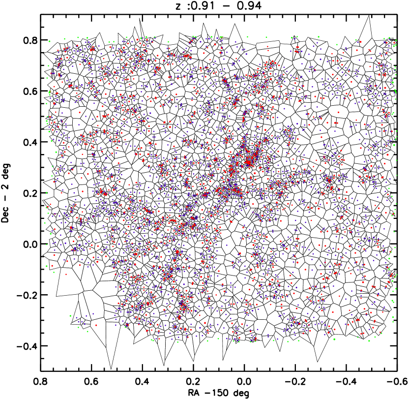
Figure 6: The galaxy density field is shown for a sample redshift slice at z $=0.93$ with the width ($\Delta z=0.03$) of the slice matching the accuracy of the photometric redshifts for the selected galaxy sample. The Voronoi 2-d polygons outline the area closest to each individual galaxy. In the tessellation diagrams the individual galaxies are shown as red or blue points depending on the SED type of the galaxy (early and late, respectively), clearly showing the correlation of early type galaxies with denser environments at these redshifts. (Green points indicate galaxies on the outside of the area for which the Voronoi polygons are not closed.) The sparse region in the lower left corner is a masked area where the Ultra-Vista coverage was incomplete (see Fig. 29). Animation 1 shows the galaxies distribution which was the basis for the derived densities and full sets of the voronoi plots for the 127 redshift slices are available in animation 2 in the electronic edition of the Astrophysical Journal.

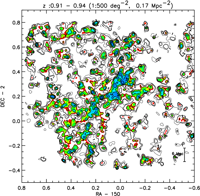
Figure 7: The density field estimated from the inverse area of each galaxy shown in Fig. 6. The vertical bar in the lower right indicates the comoving scale length of 6 Mpc. Contours are at : 1, 2 , 5, 10, 20, 50, 100, 200 and 500 times the density units (per deg² and per Mpc²) given in the upper legend of the plot. Full sets of these plots for the 127 redshift slices are available in animation 3 in the electronic edition of the Astrophysical Journal.

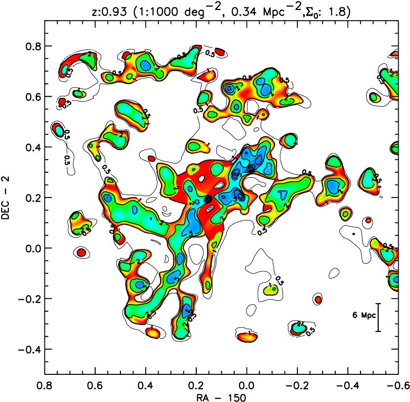
Figure 8: Statistically significant overdense regions (relative to the mean density at the same redshift) are shown from adaptively smoothing the spatial distribution of galaxies in redshift slice at z $=0.93$ (see Fig 6). The vertical bar in the lower right indicates the comoving scale length of 6 Mpc. Contours are at : 0.5, 1, 2 , 5, 10, 20, 50, 100, 200 and 500 times the density units (per deg² and per comoving Mpc²) given in the upper legend of the plot. The mean density given by $\Sigma_{0}$ in the upper legend has been removed before computing the overdensity. Full sets of these plots for the 127 redshift slices are available in animation 4 in the electronic edition of the Astrophysical Journal.

4 COSMOS LSS

Figures 6 – 8 show the derived density fields of galaxies and overdensities for the selected redshift slices. From the tessellation analysis, both the Voronoi polygons for each galaxy (color coded red for early-type SEDs and blue for late-type or starburst SEDs) and the derived density fields are shown. Statistically significant overdensities are revealed from the adaptively smoothed surface densities in Fig. 8. These figures illustrate well the spatial clustering of the galaxies which can be seen in COSMOS using accurate photoz to remove foreground and background galaxies for each redshift. In each redshift slice many overdense structures are seen – both dense ’circular clumps’ and elongated filamentary structures. The routine detection of the filamentary structures at most redshifts is a new feature provided by COSMOS – enabled by the large galaxy samples having high accuracy photometric redshifts. The very large samples of galaxies available through photometric redshifts enable the mapping of structures even at relatively low densities. [Areas masked due to bright stars contaminating the photometry are shown in Fig. 29 and these appear as blank regions in the LSS at all redshifts.]

In Figure 9, the adaptively smoothed and Voronoi projected surface densities are shown for selected ranges of redshift. These images were made by summing the densities over the range of redshifts specified on each plot. In general, there is extremely good correspondence between the structures derived using the two techniques after allowing for their different objectives and strengths : the adaptive smoothing picks up only statistically significant overdensities while the Voronoi technique shows all overdensites and is less shape and scale dependent. Approximately 250 significantly overdense regions are detected with scales 1 to 30 Mpc (comoving). We did not attempt to catalog the separate structures – tracing their full extent and deciding whether multiple peaks are really part of a single larger structure becomes quite subjective. (Automated delineation of the structures was attempted with only limited success; the parameters appropriate to different redshifts must be changed as a function of redshift, due to the varying levels of confusion and thus, the resulting catalogs are non-uniform in their selection biases.)

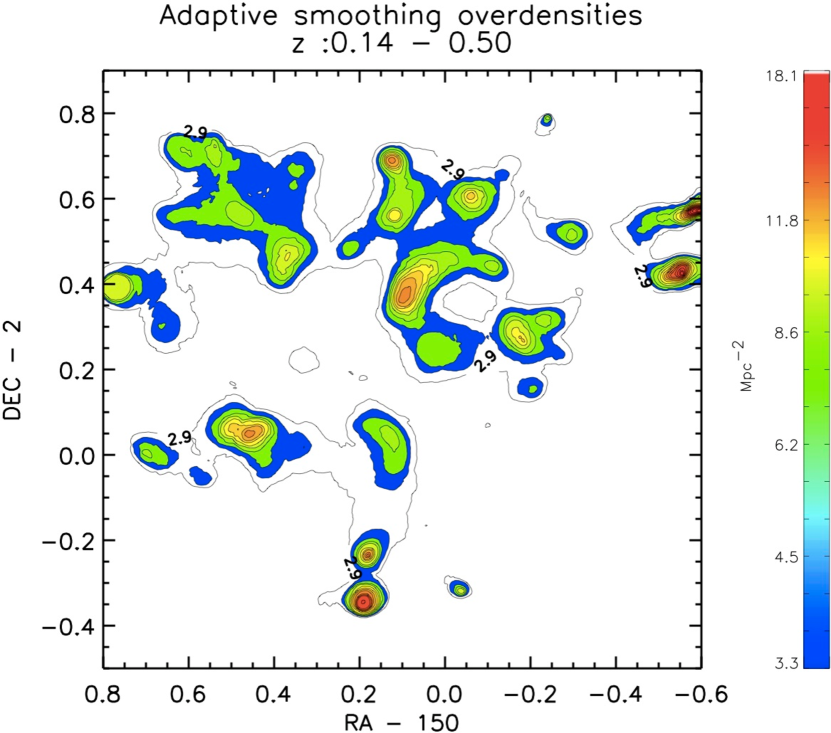
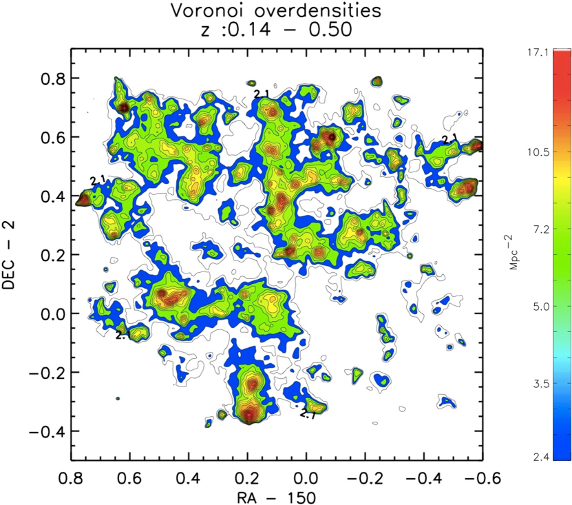
Figure 9: Overdense regions at z = 0.14 - 0.5 are shown for the adaptive smoothing (Top) and Voronoi (Bottom) techniques. The images were made by summing the derived overdensities measured from the individual redshift slices. The numbers on the lowest uncolored contour correspond to the projected density in Mpc^-2.

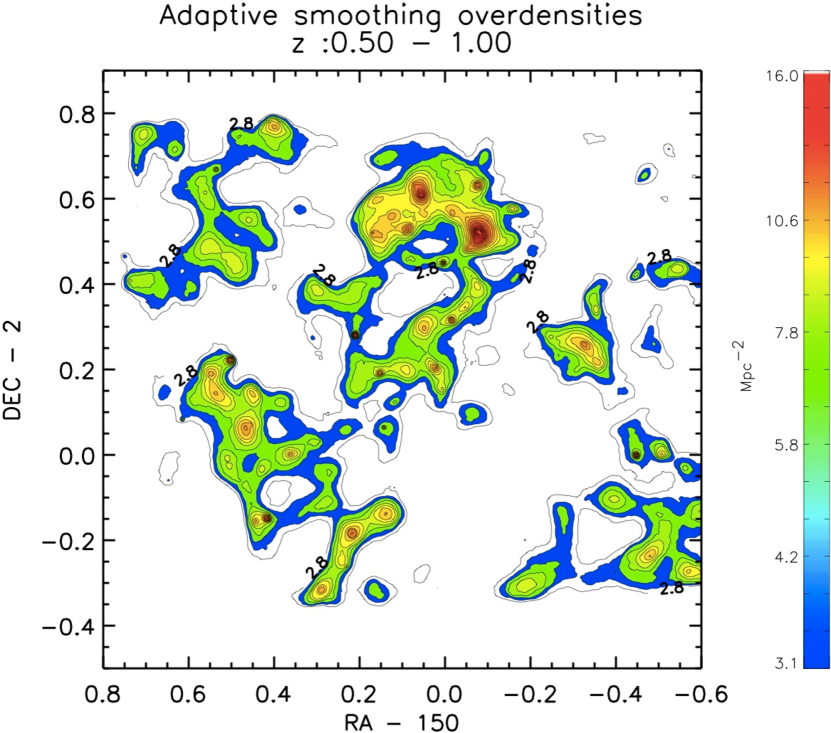
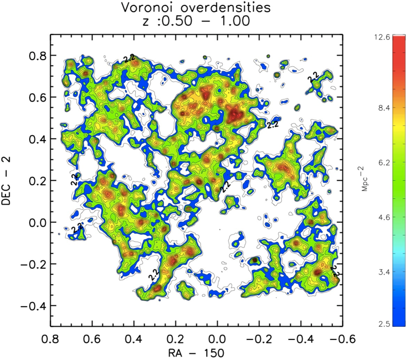
Figure 9 b: Overdense regions at z = 0.5 - 1.0 are shown for the adaptive smoothing (Top) and Voronoi (Bottom) techniques. The most massive structure in COSMOS at z = 0.73 can be seen here in the top center (Guzzo et al., 2007; Cassata et al., 2007).

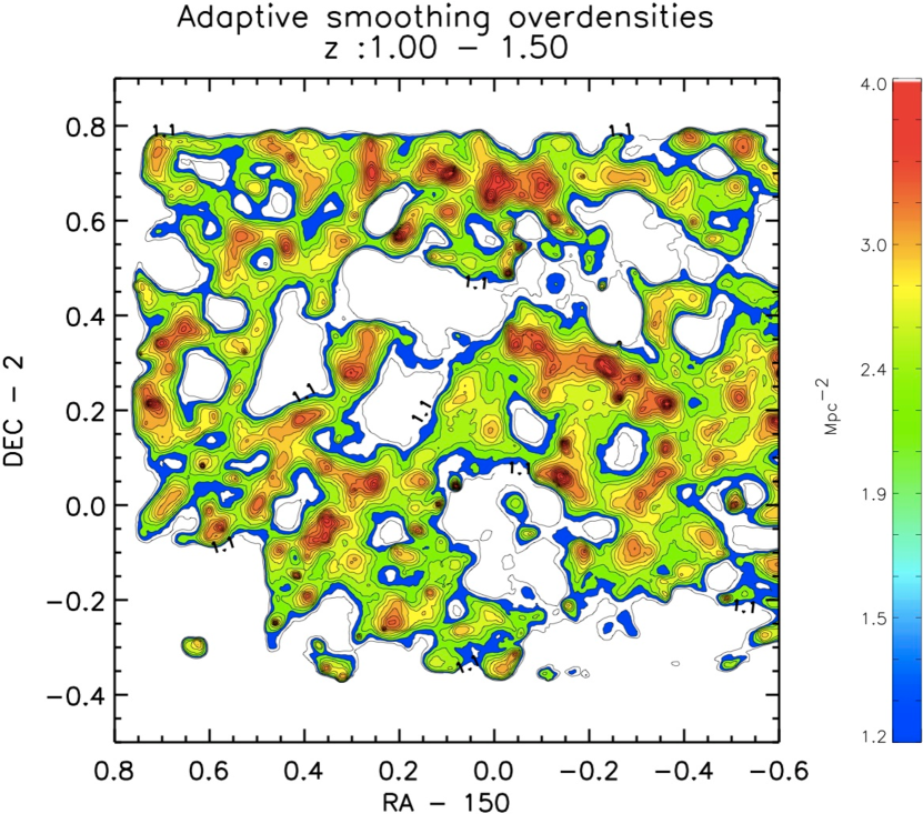
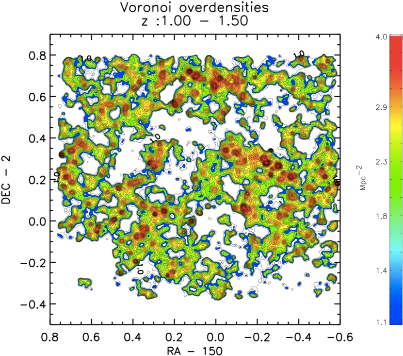
Figure 9 c: Overdense regions at z = 1.0 - 1.5 are shown for the adaptive smoothing (Top) and Voronoi (Bottom) techniques.

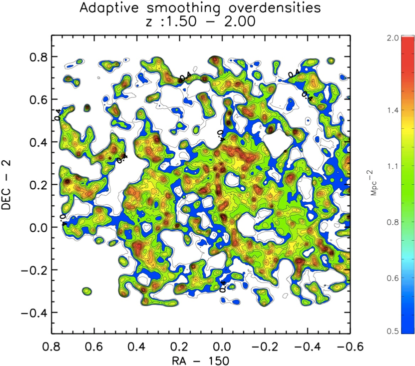
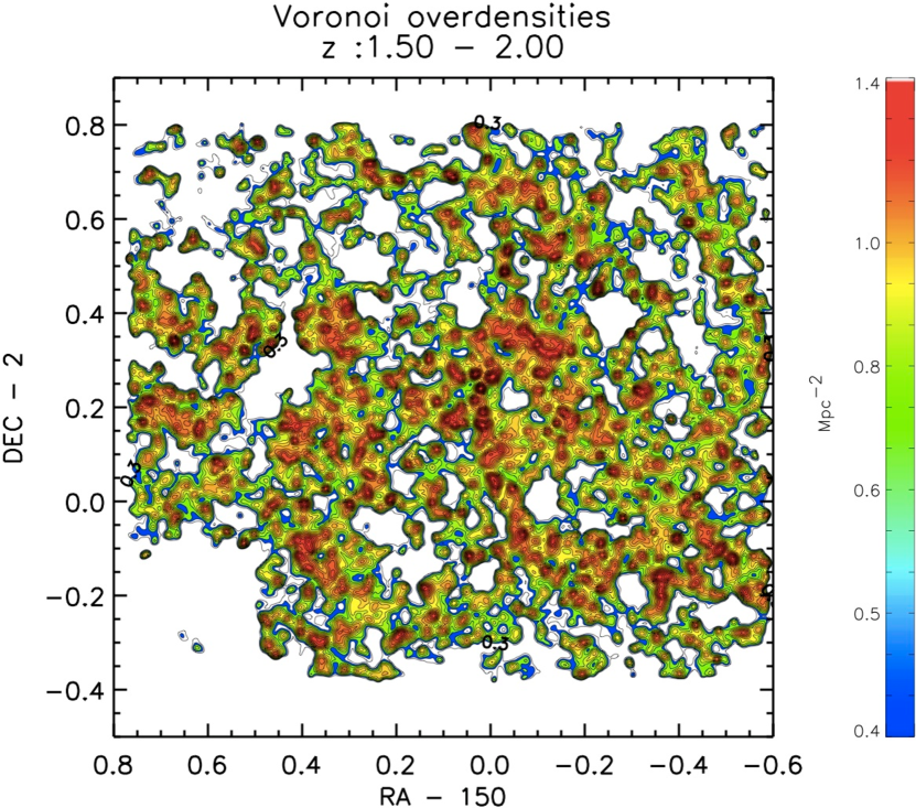
Figure 9 d: Overdense regions at z = 1.5 - 2.0 are shown for the adaptive smoothing (Top) and Voronoi (Bottom) techniques.

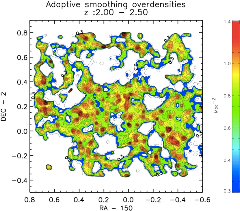
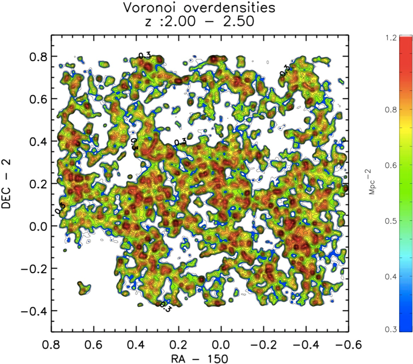
Figure 9 e: Overdense regions at z = 2.0 - 2.5 are shown for the adaptive smoothing (Top) and Voronoi (Bottom) techniques.

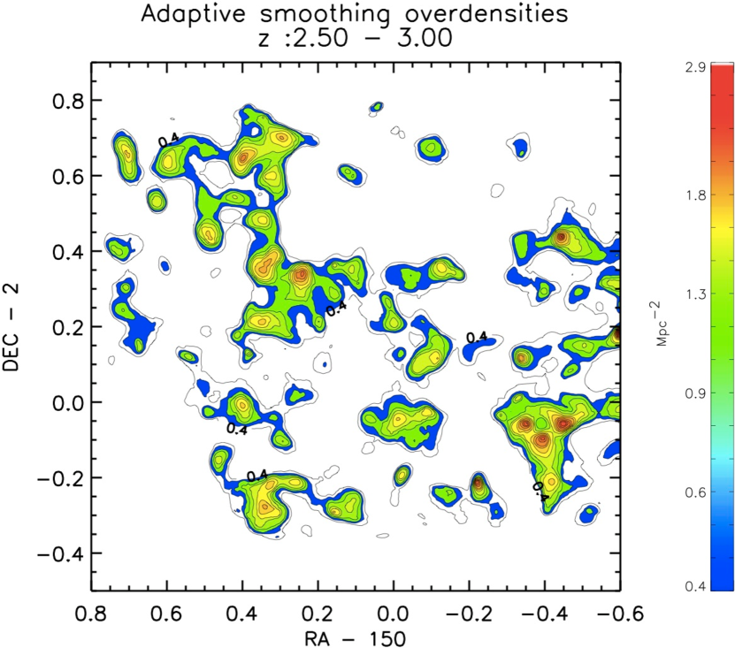
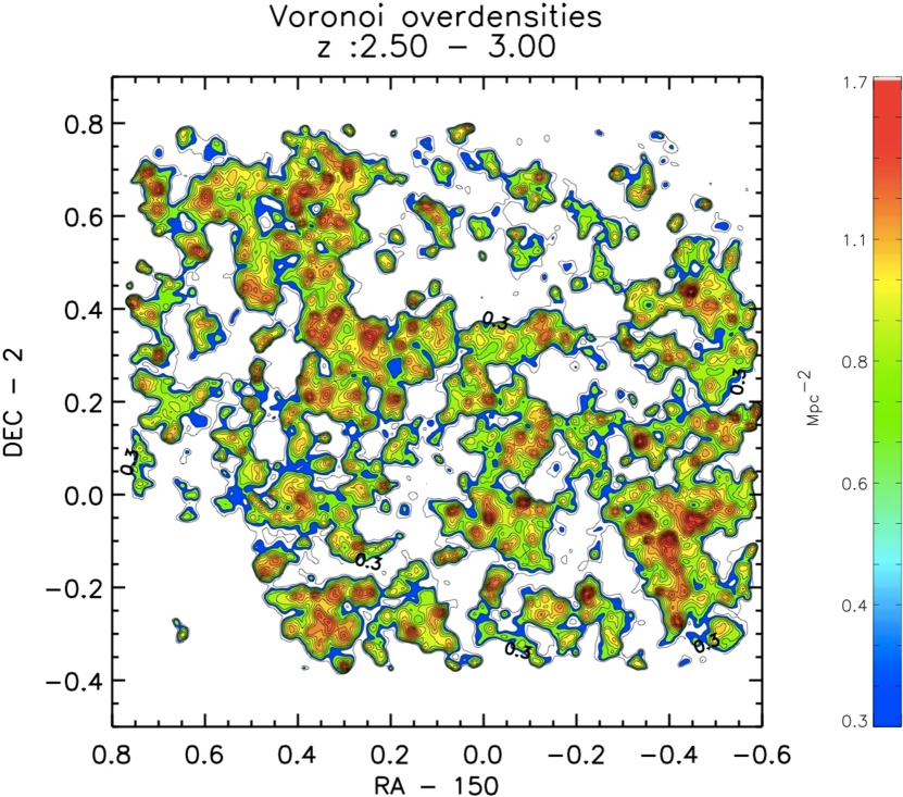
Figure 9 f: Overdense regions at z = 2.5 - 3.0 are shown for the adaptive smoothing (Top) and Voronoi (Bottom) techniques.

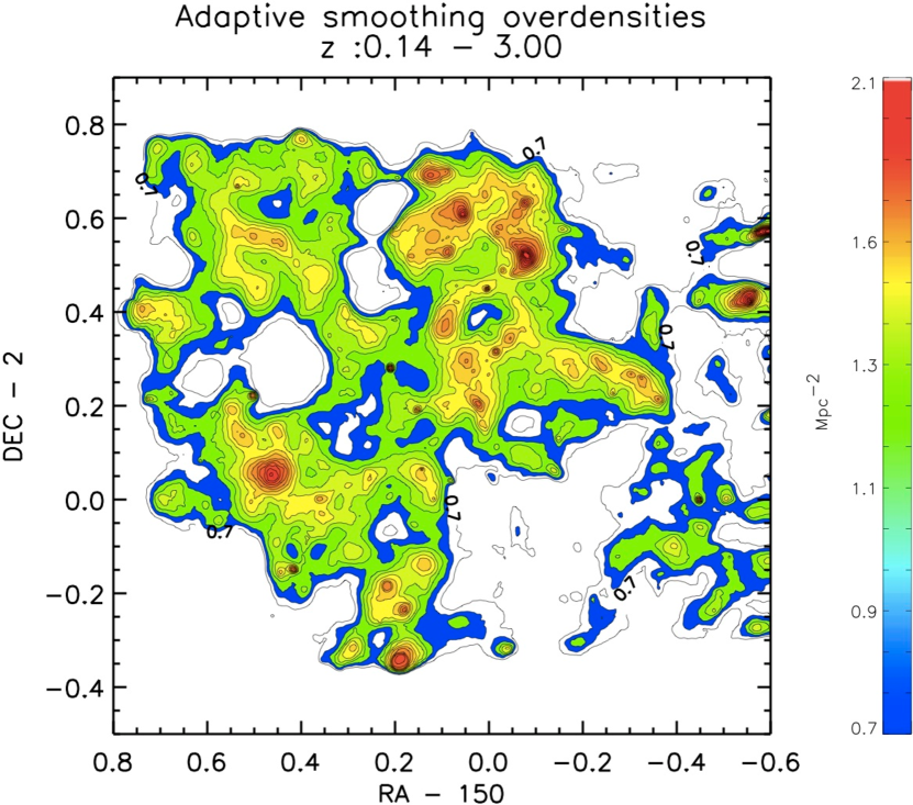
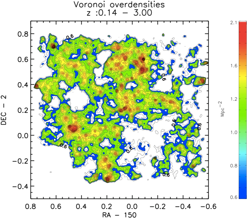
Figure 9 g: Overdense regions for the full redshift range at z = 0.15 - 3.0 are shown for the adaptive smoothing (Top) and Voronoi (Bottom) techniques.

5 Evolution of COSMOS LSS and Comparison with the Simulation

Figure 16 shows the range of environments for the COSMOS sample as a function of redshift. The contours indicate relative numbers of galaxies as a function of environmental density and redshift. Overall, we find excellent correspondence between the COSMOS sample and that from the simulation – both in the relative number of galaxies at different environmental densities and the variation of the structure densities with redshift (see below).

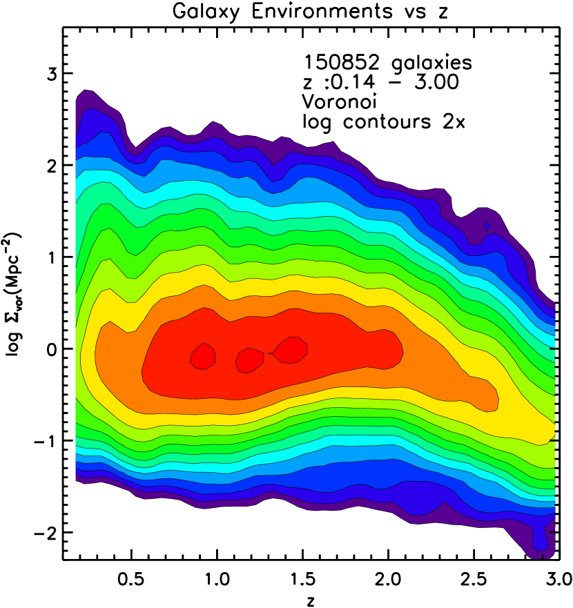
Figure 16: The densities measured with the Voronoi technique are shown for the sample of 150,852 COSMOS galaxies from z = 0.14 to 3.0. At low z, these densities extend over 3 orders of magnitude, typically from 0.1 to over 100 Mpc^-2 and at the highest z approximately 2 orders of magnitude. The contours, showing the relative numbers of galaxies at each density and redshift, decrease by a factor of 2 for a full range of 1/4096 at the outermost contour level. At high redshift, the decrease in the number of galaxies at high densities is due to cosmic evolution of the density field (see Fig. 3).

The LSS seen in COSMOS and those in the $\Lambda$CDM simulation can be compared by measuring the fractional area occupied by environments of varying overdensities. For the simulation, the redshifts were given the same dispersion as the COSMOS photoz (see Fig. 2) and the structures were measured using the same techniques as discussed in §2.3 In Fig. 17, this area filling percentage is shown as a function of overdensity for 4 redshift ranges. This figure clearly illustrates the increasing range of overdensities seen at low redshift compared to higher redshifts. The figure also shows extremely good correspondence in the area filling fractions and their evolution with redshift between COSMOS and the simulation. This area filling percentage is analogous to a spatial power spectrum, but perhaps more easily visualized. The relative frequency of a given overdensity at each redshift is more directly apparent than would be the case for a power spectrum.

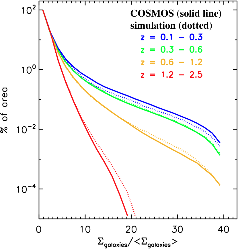
Figure 17: The percentage of area on the sky occupied as a function of environmental overdensity for selected redshift ranges is compared between the COSMOS data and WMAP3YC simulation for areas with significant overdensity. The simulation very accurately reproduces the relative amounts of structure as function of both environmental density and the evolution of this structure.

6 Correlation of Galaxy Properties with Environment

A major motivation of this study is the exploration of the environmental influence on galaxy properties – their SED types, star formation rates (SFR) and stellar masses. Given the well-known correlation of early type massive galaxies with dense/cluster environments at low redshifts, we can now investigate at which redshifts these influences develop, and explore in more detail the dependence on environmental density, using the enormous galaxy samples in COSMOS. And since similar processing has been employed on the simulation, we can compare in detail the observations with the semi-analytic model predictions.

6.1 Galaxy Colors and SED Types

In Figure 18 the correlations of galaxy SED type (§2.2) with density and redshift are shown. For each redshift-density cell, the color fractions are proportional to the fraction of each galaxy type. In the left panel, the galaxy number fraction is shown and in the right panel each galaxy is weighted by its mass. As noted earlier, the correspondence between the rest-frame b-i color and the galaxy type is taken from Arnouts et al. (2007) and the stellar mass from the COSMOS photoz catalog was estimated using a color dependent mass-to-light ratio (see Ilbert et al., 2009).

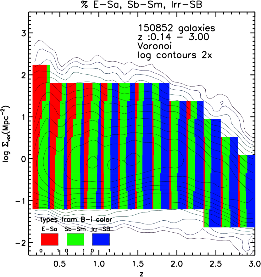
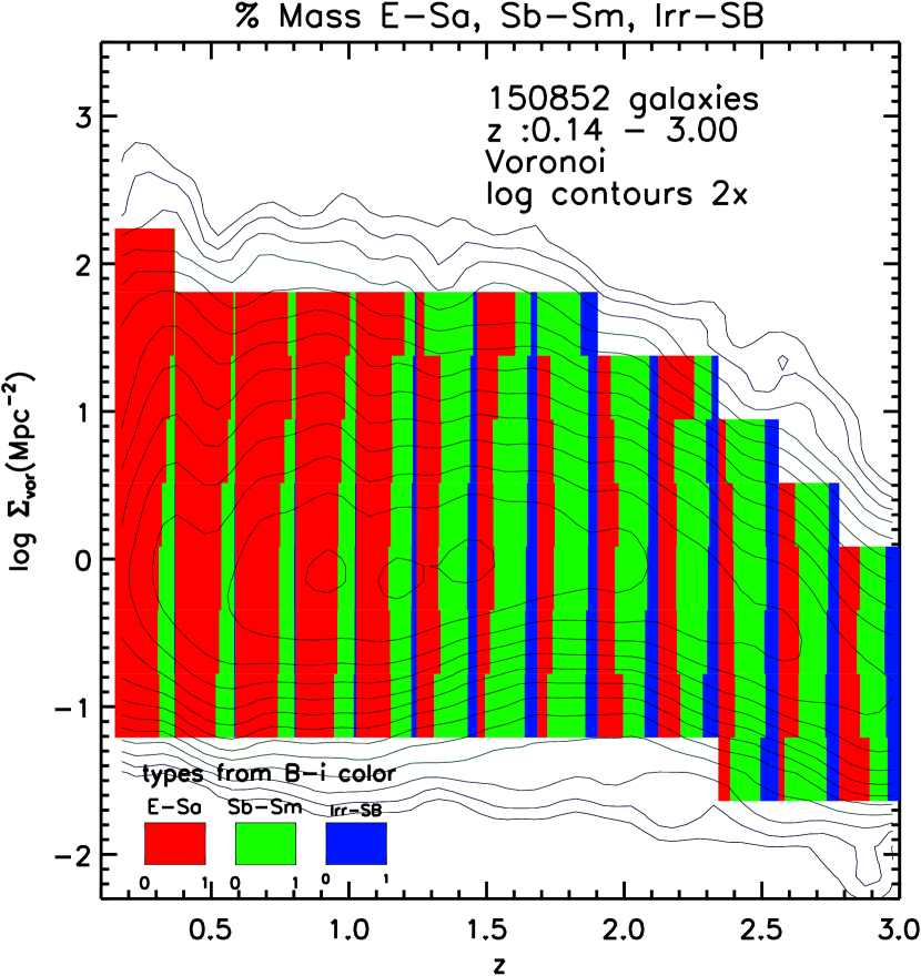
Figure 18: Galaxy percentages in COSMOS (classified as early-type (E-Sa), Spiral (Sab-Sd) and IRR/SB on the basis of their rest-frame reddened b-i colors) are shown as a function of environmental density and redshift. The left panel shows the percentage by number and the right panel weights each galaxy by its mass.

Figure 19: The correspondence between the density percentiles (used in Fig. 20 - 24) and the absolute surface density per comoving Mpc² is shown for 7 redshift ranges in COSMOS.

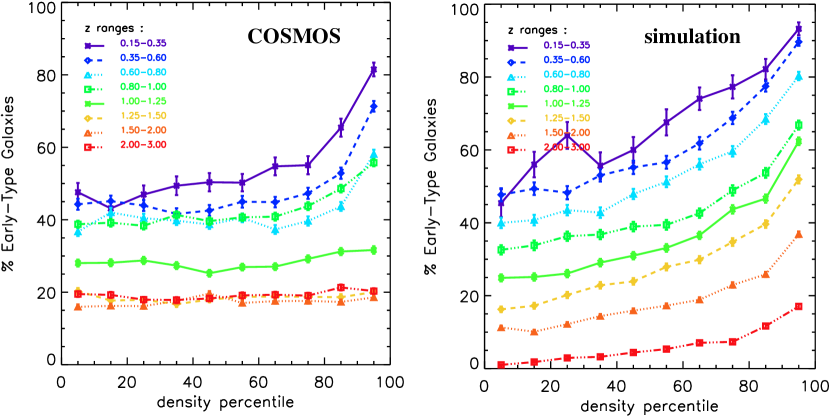
Figure 20: The percentage of Early type galaxies (E-Sa) as a function of environmental density percentiles is shown for 8 redshift ranges for COSMOS galaxies (Left) and simulation (Right). At each redshift, the distribution of environmental densities is calculated and each galaxy’s percentile within that distribution is determined. This effectively normalizes out the lower range of environmental densities at high redshift and the redshift dependence of the mean environmental density. The error bars show the dispersion in the median estimates for the sample in each bin; when the error bars are not shown, they are smaller than the symbol. The uncertainties shown in these and subsequent figures are calculated by bootstrap resampling. The translation between density percentile and actual surface density of galaxies is shown in Fig. 19.

Numerous studies have shown a strong dependence of the red galaxy fraction on environmental density at low redshift (e.g. at $z<0.1$ Baldry et al., 2006). Figures 18 and 20 clearly show a strong preference for the early type galaxies to inhabit the denser environments out to $z\sim 1.2$ although their total percentage decreases systematically with increasing z. Beyond $z\sim 1.2$, the early type galaxies are much less numerous and the strong environmental correlation disappears. Iovino et al. (2010) analyzed the blue galaxy fraction in galaxy groups defined from the zCOSMOS spectroscopic sample and found a strongly increasing blue fraction at higher redshifts.

To more clearly show the correlations with relative density as a function of redshift, we classify each galaxy by where it falls within the distribution of LSS densities at its redshift. At each redshift, the distribution of environmental densities is calculated and each galaxy’s percentile within that distribution is determined. This effectively normalizes out the lower range of environmental densities at high redshift, and the redshift dependence of the mean environmental density. The translation between these density percentiles and absolute surface density is shown in Fig. 19.

Figure 20 shows the variation in the percentage of early type galaxies (with SED corresponding to E-Sa galaxies) with density percentiles for 8 redshift ranges. This plot clearly shows the steep increase in the fraction of early type galaxies at z $<1.2$ and the development of strong environmental dependence at the same time, starting at $z\sim 1.2$ in the observed galaxies. For the simulation galaxies, the environmental dependence for the early type galaxies persists all the way out to z = 3, albeit with reduced strength (Fig. 20 - right). The flattening of the density dependence in the early type fraction at the highest redshifts is likely due in part to the reduced dynamic range of environmental densities at high z (see Fig. 19) and the fact that at early epochs the evolution is driven by environment on smaller scales. Another notable difference between the COSMOS and simulation samples is the overall lower fraction of early type galaxies in the simulation at z $>1.5$. In summary, the most notable difference between the simulation and the COSMOS galaxies is that the simulation shows higher percentages of early type galaxies in the dense environments and smoother and more regular variations – probably an expected result of the strictly prescriptive semi-analytics.

In the following, we refer to this transition in the density dependence for the observed galaxies as the ’Emergence of the Red Sequence’. This is not to imply that red sequence galaxies do not exist at higher redshift, simply that they do not exhibit the clear density dependence seen at $z<1.2$. The span of cosmic age over which this emergence takes place is only $\sim 1$ Gyr. It is important to emphasizes that the simulation, which was subjected to the same redshift uncertainties, photometric selection and LSS mapping techniques, did in fact show environmental dependence all the way to z = 3, so the emergence of the environmental dependence in the observed galaxies only at $z\sim 1.4$ is not due to any selection or measurement effect.

6.2 Star Formation Activity

The SFRs for each of the galaxies were estimated from the rest-frame NUV continuum of their SEDs and corrected for extinction, combined with SFR estimates from Spitzer 24$\mu$m data as described in §2.2. In Fig. 21 the median SFRs and star formation timescales ($\tau_{SF}=M_{*}/SFR$) are shown as a function of redshift and environmental density. For both quantities, extremely strong environmental dependence is seen at low redshift with a factor of 10 change in both the SFR and timescale between the average at low z and that seen in the densest environments. As with the early type galaxy fraction, the environmental segregation falls off and disappears above z $\sim$1. In Fig. 21 it can be seen that the median SFRs perhaps show some a very mild environmental dependence out to $z\sim 3$ but it certainly not as significant as the correlation at low z. At $z<0.1$ using SDSS, Kauffmann et al. (2004) found a strong dependence of the specific star formation rate ($sSFR=SFR/M_{*}=1/\tau_{SF}$) with environment – a factor 10 decrease in the sSFR going from low to high density environments.

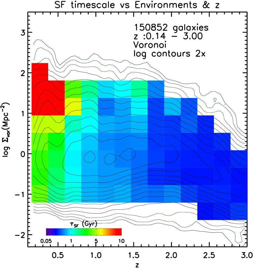
Figure 21: The median SFR (Left) and star formation timescale ($\tau_{SF}=M_{*}/SFR$) (Right) for COSMOS galaxies are shown as a function of environmental density and redshift.

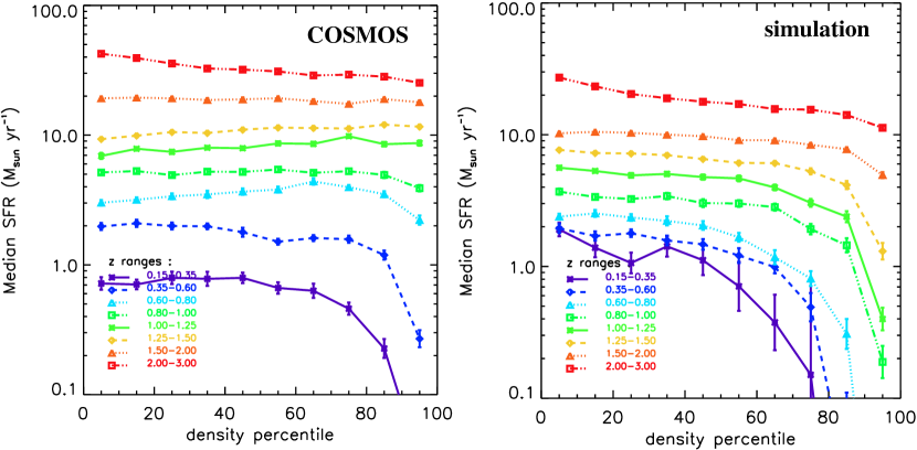
Figure 22: The median SFR as a function of environmental density percentile for 8 redshift ranges for COSMOS galaxies (Left) and Millennium (Right). The error bars show the dispersion in the median estimates for the sample in each bin; when the error bars are not shown, they are smaller than the symbol.

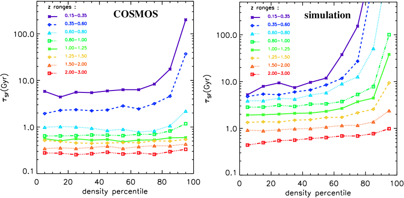
Figure 23: The characteristic SF timescale ($\tau_{SF}=M_{*}/SFR$) is shown for 8 redshift ranges for COSMOS galaxies (Left) and Millennium (Right). The error bars show the dispersion in the median estimates for the sample in each bin; when the error bars are not shown, they are smaller than the symbol.

In Figure 22, the median SFRs are shown for the COSMOS and simulation galaxies as a function of environmental density and redshift. The observed galaxies exhibit a significantly stronger increase in SFRs with redshift than those in the simulation, but somewhat weaker environmental dependence at the lowest redshifts. The COSMOS SFRs increase by a factor of $\sim 40$ from z =0.1 to 2.5 while the galaxies in WMAP3YC show median SFRs up by a factor of $\sim 25$ over the same range. Both the observed galaxies and those in the simulation also exhibit strong environmental dependence out to z $\sim 1.0$ and 1.2 respectively. Figure 23 shows the variation in the characteristic star formation timescale (i.e. the median $\tau_{SF}$) – this star formation timescale by an order of magnitude increase from z $=3.0$ to 0.15 in less dense environments, and two orders of magnitude decrease in the denser environments.

In recent work, there has been major divergence regarding the dependence of the SFR in galaxies on their environment at $z\sim 0.8-1$. In the local universe, several investigations find the mean SFR of galaxies in dense environments to be much less than those of galaxies in lower density regions (Gómez et al., 2003; Balogh et al., 2004; Kauffmann et al., 2004). Elbaz et al. (2007) and Cooper et al. (2008) have suggested a reversal at $z=0.8-1$ of the SFR-density relation (i.e. higher SFRs at higher densities); however, (Patel et al., 2009) found no such reversal for a cluster and its environment at $z=0.1274$. We see no evidence of the claimed reversal in the density dependence using our sample of galaxies which is larger by a factor of 10-100 than those in the above studies and with consistent density estimators for the entire redshift range. (The basis of the reversal noted by Cooper et al. (2008) is hard to assess since the effect shown in their Fig. 12d is not clearly evident in Fig. 12b which plots the observed points from which Fig. 12d is derived.) As noted by Patel et al. (2009), the reversal claimed by Elbaz et al. (2007) actually occurs only in a narrow range of density and not at the very highest density. Using zCOSMOS data, Cucciati et al. (2010); Bolzonella et al. (2010) also see no reversal. Using [OII] emitters at $z\sim 1.2$ detected in narrow band imaging in COSMOS, Ideue et al. (2012) found that the average SFR of star-forming galaxies was independent of both stellar mass and environmental density, consistent with our results at this and higher redshifts.

6.3 Environmental Dependence of the Star Formation Rate Density

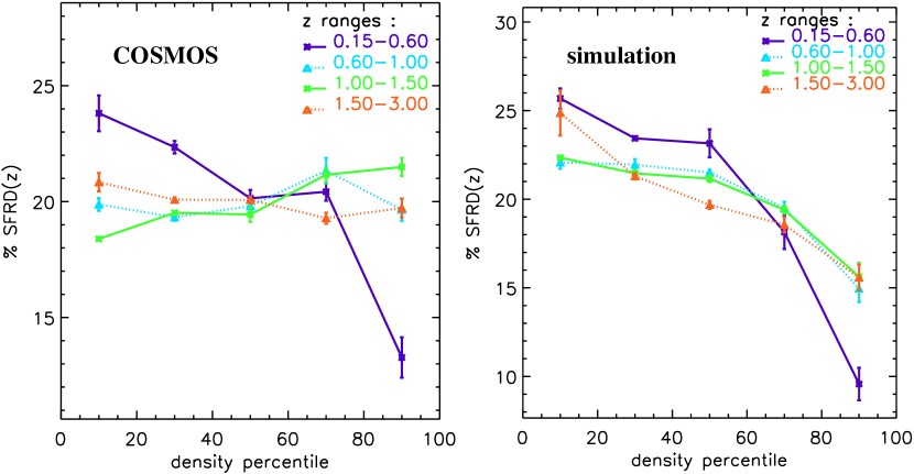
Figure 24: The percentage of the star formation rate measured at each redshift attributed to different percentiles of the environmental density. The Left panel shows the COSMOS data; the Right shows the simulation SFRD. At high redshift the SFRD is distributed equally across the density percentiles but at z $<0.6$ the major contributions arise in the lower density environments.

It is now well established that the total SFR per unit of comoving volume or star formation rate density (SFRD) evolves strongly with cosmic time, decreasing by a factor of $\sim 20$ from z = 2 to 0 (see Karim et al., 2011, and references cited there). Using the environmental densities derived here, it is possible to investigate how the SFRD at each epoch is distributed with environment. In Fig. 24, the relative contributions to the total measured SFR(z) of galaxies in the different density percentiles are shown. Since there are, by construction, equal numbers of galaxies in each density percentile bin, this plot normalizes out the redshift variation of the number of galaxies in different density regimes. Fig. 24 shows that the SFRD is uniformly distributed amongst the density percentiles at all redshifts z $>$ 0.6, while below that redshift the SFRD shifts strongly to galaxies in lower density environments. Remarkably similar behavior is seen in the COSMOS (left panel) and simulation galaxies (right panel).

The preferential shift of the SFRD to lower density LSS is probably a result of two factors: 1) the galaxies in the high density regions evolved earlier and 2) the shutdown of resupply of star forming gas in the dense environments (where the galaxy velocity dispersions are higher, and feedback could halt the diffuse gas accretion, see §6.5). It is worth noting that since the mean stellar masses of galaxies in the dense environments are significantly higher, even above z = 0.6, the mass weighted SFRD would show even earlier environmental variation than the number-weighted SFRDs shown in Fig. 24.

6.4 Buildup of Stellar Mass in Passive and Star Forming Galaxies

The SEDs of galaxies at $z<3$ are separable into two distinct classes: the so-called Red Sequence (Early type) galaxies with relatively low rates of on-going SF, hence called passive galaxies; and the Blue Cloud (Late type) galaxies with high SF rates. In color-magnitude diagrams, there is a much lower number of galaxies in the Green Valley between the Red Sequence and Blue Cloud. Rather than the standard color-magnitude diagram, we show in Fig. 25 this bifurcation of galaxy populations in more physical units: the maturity, $\mu=\tau_{SF}/\tau_{cosmic}=(M_{*}/SFR)/\tau_{cosmic}$ where $\tau_{cosmic}$ is the age of the universe at each redshift. Since we are interested in the relative maturity of galaxy stellar populations over a range of redshift, we have normalized the SF timescales by the cosmic age at each redshift. The star formation timescale is estimated using the SFRs (from the UV continuum plus the IR, see §2.2) and stellar masses; hence, the maturity responds rapidly to changes in the SFRs. (The UV continuum at $\sim 1800$Å is produced by OB stars. For an instantaneous starburst with a Kroupa stellar IMF, the UV will fall by a factor of 10 within $30\times 10^{6}$ yrs after the starburst ends (Scoville & Li, 2011).) Fig. 25 shows the variation of the galaxy populations as a function of environmental density (left panels, low density and right panels, high density) and redshift (the rows) from $z=0.15$ to $3.0$. The dashed line in the figures is the approximate color-dependent mass limit corresponding to the photometric selection function.

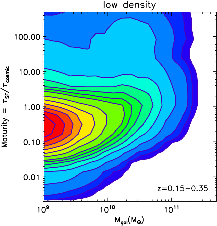
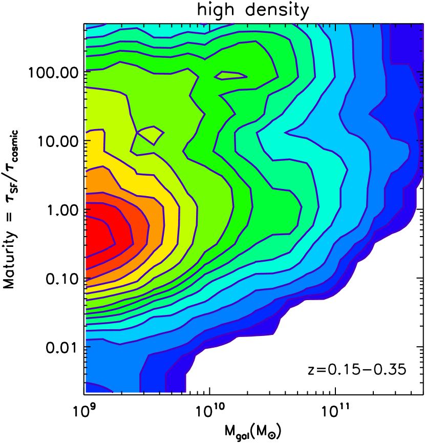
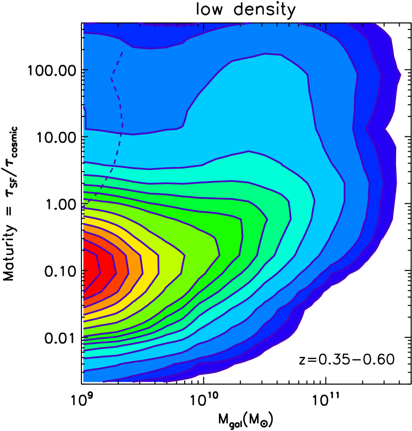
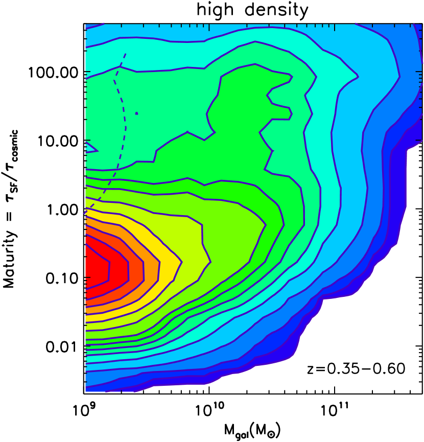
Figure 25: The maturity ($\tau_{SF}/\tau_{cosmic}$) is shown separately as a function of stellar mass for low (left panel of each pair) and high (right panel of each pair) density environments as a function of redshift (pairs of panels). The maturity is correlated with the rest frame colors of the galaxies (primarily the NUV for the SFR and the near infrared for the stellar mass). At low redshift, the maturity shows extremely good separation of the blue cloud and red sequence galaxies. On each plot the dashed line indicates the mass limit of the selection function as a function of maturity. (These mass limits are the average for objects in each redshift range and hence, some galaxies at the low end of the redshift interval will appear to the left of the mass limit line.) Contours at : 0.05, 0.1 ,0.15 ,0.2, 0.25, 0.3, 0.4, 0.5, 0.6, 0.7, 0.8, 0.9 $\times$ peak. The high and low environmental density bins are such as to split the overall galaxy sample in half at each redshift.

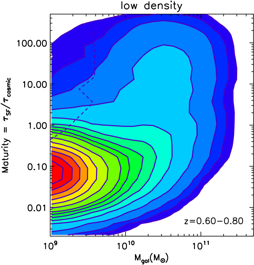
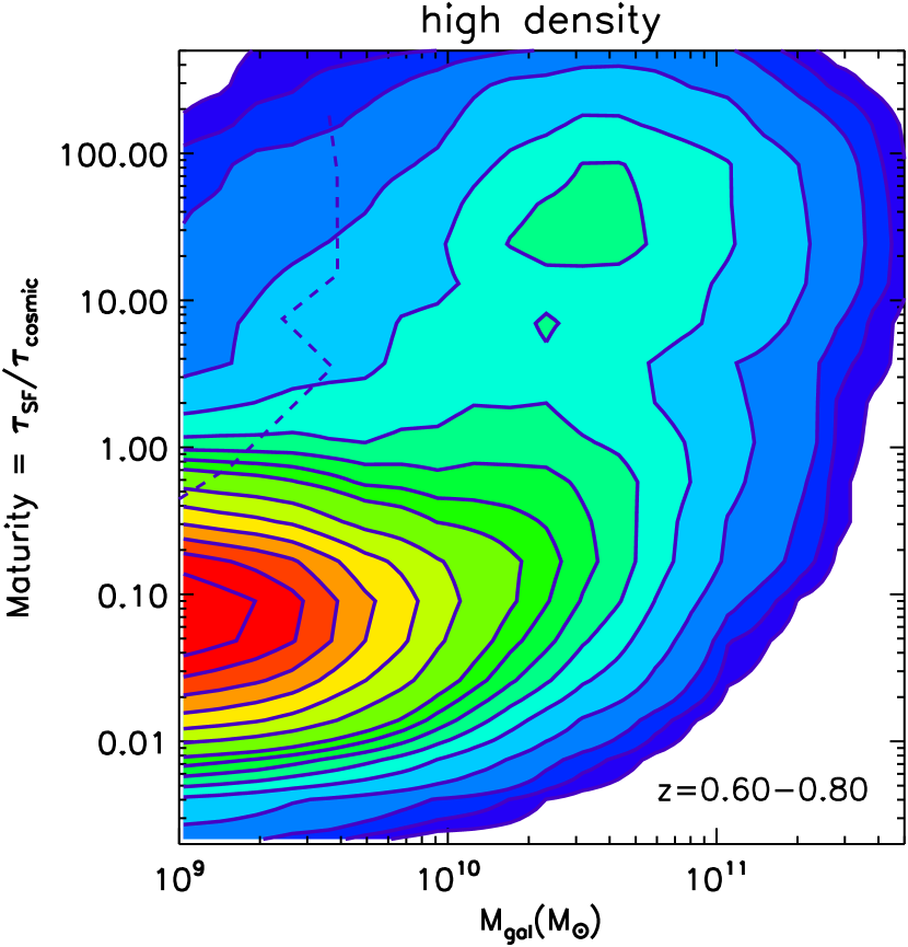
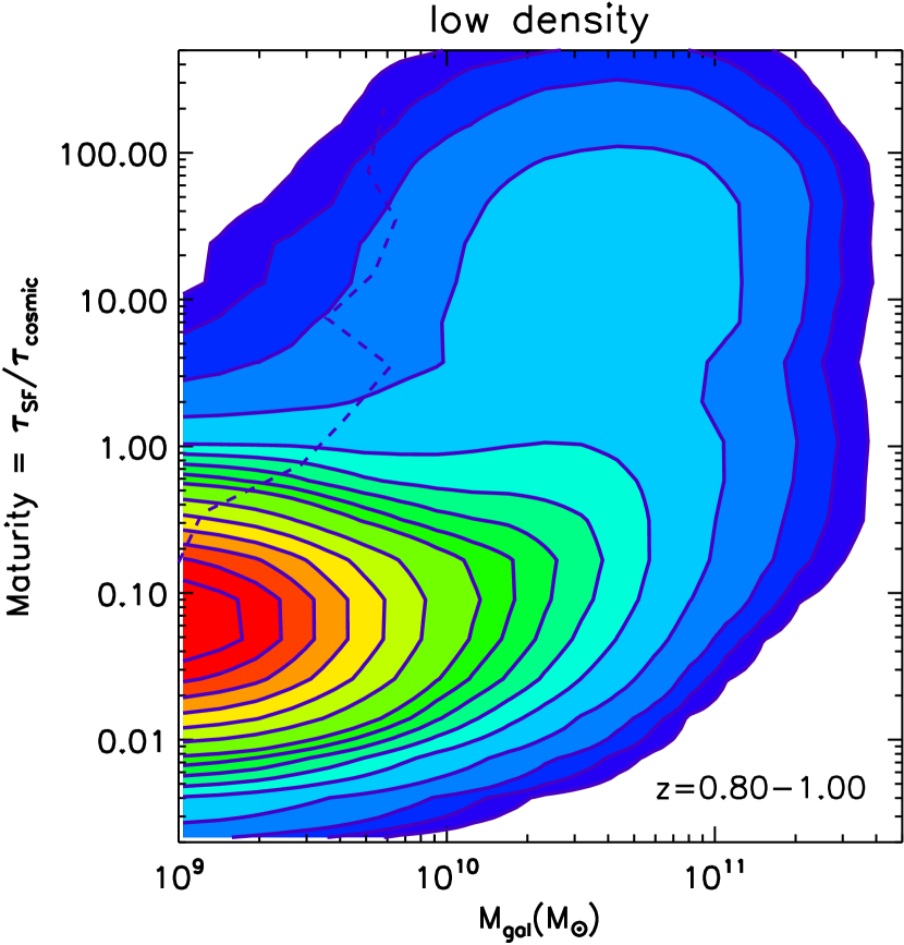
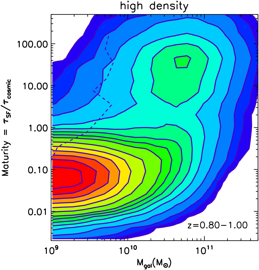
Figure 25 b: continued

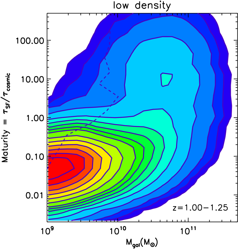
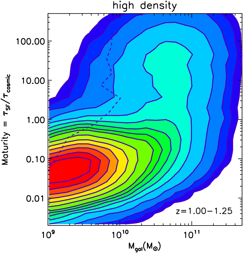
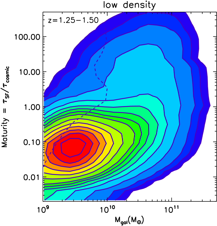
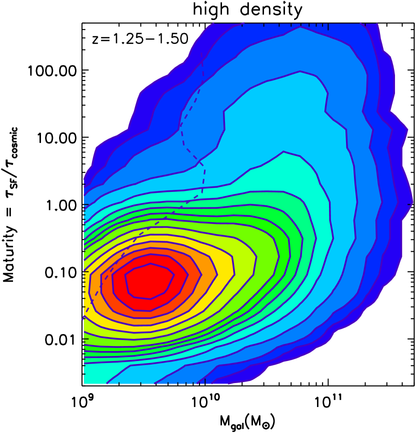
Figure 25 c: continued

At low z, Fig. 25 shows very clear separation of the Red Sequence (Maturity $\mu>10$) and Blue Cloud ($\mu\lesssim 2$) and an enhancement of the Red Sequence in the denser environments (right panel). In the Green Valley, between the Red Sequence and the Blue Cloud, the number density of galaxies (in the mass-maturity plane) is as low as 30% of the peaks on either side. This enhancement of the Red Sequence in denser environments persists but with diminishing amplitude out to $z=1$. In these plots, the Red Sequence clearly extends to lower mass galaxies at decreasing redshift. In fact, comparing the plot for z = 0.15 - 0.35 and z = 0.35 - 0.60 (Fig. 25 a), a major development is the appearance of the low mass red galaxies at z = 0.15 - 0.35, which were not very apparent at z = 0.35 - 0.60. This strongly implies that such galaxies are the result of environmental quenching processes (such as ram pressure stripping or starvation of gas accretion) rather than dry merging since the lower mass red galaxies were not present in sufficient abundance at the earlier epoch. This corresponds to the environmental quenching as discussed by Peng et al. (2010).

The mass limit cutoff shown by the dashed line in each panel is at significantly lower mass than the mass at the peak of the Red Sequence, and therefore the disappearance of environmental dependence of the Red Sequence at $z>1.1$ is not due simply to insufficient mass sensitivity for passive galaxies. Additionally, we note that such effects would not differentiate between low and high density environments. Thus, we conclude that environmental differentiation decreases at the higher redshifts.

A more complete analysis of the galaxy mass function evolution is provided by Ilbert et al. (2009). The Red Sequence shows an obvious tilt in maturity as a function of stellar mass (Fig. 25-a), implying that the lower mass red galaxies were built up at later times than the high mass red galaxies. This behavior is seen in the COSMOS study of galaxy mass functions (Ilbert et al., 2010) and is commonly referred to as downsizing. Above $z=1.25$, the minimum corresponding to the Green Valley disappears and the Red Sequence appears more as a plume extending out of the high mass end of the Blue Cloud (see Fig. 25 c). At $z>1.1$, one can still see a very mild environmental segregation of the Red Sequence galaxies (i.e. a slightly higher density of such galaxies in the right panel of each redshift range).

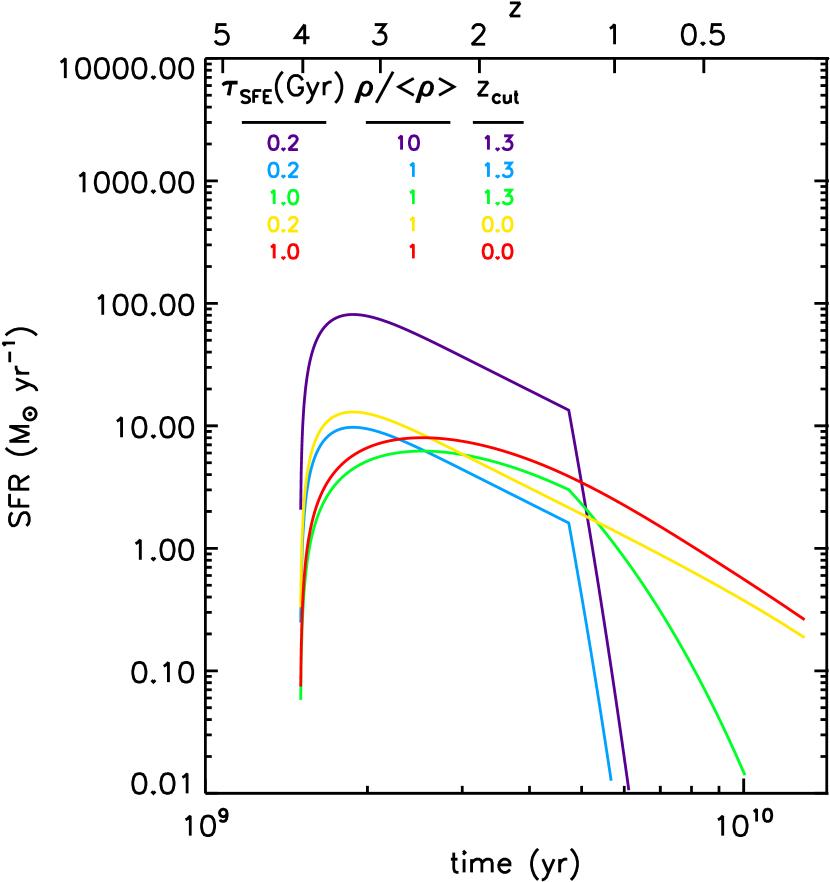
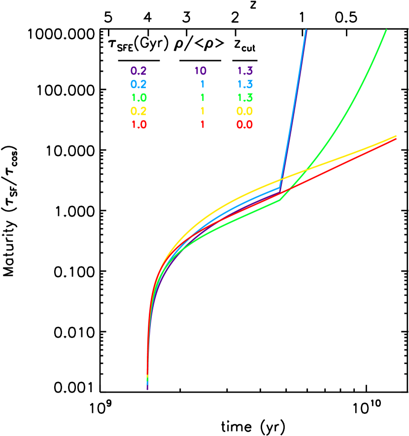
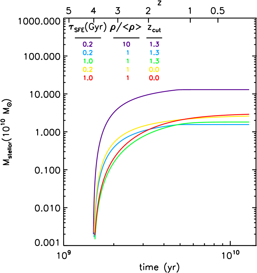
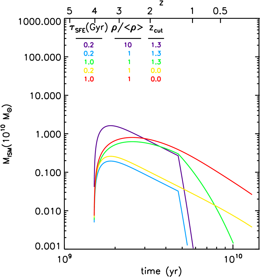
Figure 28: The SFR (upper-left), maturity ($\tau_{SF}/\tau_{cosmic}$ – upper-right), $M_{stellar}$ (lower-left) and $M_{ISM}$ (lower-right) are shown for simple models with: 1) ISM buildup by accretion from the environment (with differing overdensity); 2) varying star formation efficiencies per unit mass of ISM and 3) varying the lower redshift cutoff for the accretion (see text for details). $\tau_{SFE}=1$ Gyr corresponds to the typical efficiency observed in low-z spiral galaxies like the Milky Way; shorter timescales correspond to starburst activity. $\rho/<\rho>=1$ corresponds to the galaxy being in the average environmental density at each redshift. The accumulated stellar mass and residual ISM mass are shown in the lower two panels.

6.5 The Rapid Development of Passive Galaxies in Dense Environments

The mean cosmic ages at $z=1$ and $1.3$ are 5.7 and 4.7 Gyr, so the abrupt development of environmental segregation for passive galaxies must take place in $\sim 1$ Gyr. A number of mechanisms have been suggested for such environmental differentiation: galaxy-galaxy harassment, tidal and ram pressure stripping of the disk gas, shutoff of fresh gas accretion from the outer halo by ram pressure (’strangulation’) and feedback from starburst and active nucleus activity. To explore the possible explanations for this rapid change, we have constructed a model for the bulk evolution of galaxies with the simple assumptions that they accrete interstellar/star forming gas from their local environment and form stars with a star formation efficiency similar to that seen at low-z.

At low redshift, we may take the Milky Way as being typical of normal star forming galaxies. Here, the mass of ISM is $\sim 3\times 10^{9}$$M_{\odot}$ and the SFR is $\sim 3$$M_{\odot}$ yr^-1, implying an e-folding timescale of $\sim 10^{9}$ yrs for reducing the ISM and SFR. For the z = 1.3 star forming galaxies – ISM consumption with an efficiency or timescale like that of local galaxies will only change the Maturity (M${}_{*}/SFR/\tau_{cosmic}$) by a factor of 2 on a Gyr timescale via star formation in the blue galaxies, changing the Maturity by a factor of a few within this time period.

An alternative mechanism to populate the Red Sequence might be the merging of lower mass Red Sequence galaxies in the dense environments at $z>1.1$ (often referred to as dry merging); however, the overall mass and number of such pre-existing Red Sequence galaxies is insufficient even if the merger rate is sufficient. We are therefore forced to the conclusion that there is rapid conversion of massive star forming galaxies to passive galaxies (with SFRs decreased by a factor of $>10$ within $\sim 1$ Gyr) and the only way this can happen is by removal of the ISM.

One process which might remove the ISM rapidly and have the observed strong environmental dependence is ram pressure stripping of the ISM by cluster gas, deposited by prior star formation and AGN feedback processes. This strangulation process has been included in LSS evolution simulations by McGee et al. (2009) and they predict that the environmental dependence of the passive galaxies should set in at $z\sim 1.4-1.5$ (i.e $\sim$1 Gyr earlier than seen here).

To illustrate the need for rapid depletion of the star forming gas, we have computed the evolution for an extremely simple model in which galaxy ISM is supplied by accretion from the local environment and converted into stars at a rate or efficiency equal to that in the local universe for normal galaxies, as given above, (i.e. not undergoing a starburst). The ISM accretion or replenishment is taken to vary proportionately to the local environmental density ($\rho$) :

$$\dot{M}=\dot{M_{0}}\delta\times\rho(z)$$ (2a)

where $\delta=\rho/<\rho(z)>$ is the local environmental overdensity and $\rho(z)\propto(1+z)^{3}$ is the mean cosmic density, and $\dot{M_{0}}$ is a normalizing constant such that a significant star forming ISM has accumulated by z $\sim$ 4. This simplistic assumption is most reasonable for central galaxies but not so appropriate for satellite galaxies. The actual halo growth rate may vary as much as $(1+z)^{2.2}$ (e.g. Neistein & Dekel, 2008) and if this were adopted it would make the ISM removal problem even more severe. The accretion may occur either as spherical or cold flow accretion.

The timescale for star formation in the accreted gas is taken to be 10⁹ yr, i.e. similar to that computed above for the Milky Way (also typical of low-z spiral galaxies - Young & Scoville, 1991). This adopted efficiency is similar to that implicit to the Kennicutt relation for typical spiral galaxies (but we omit the non-linear dependence on surface density for which one would need to know the size of the ISM disk).

Using this simple model, we explore the effects of more rapid star formation or a denser environment (leading to higher accretion) on the evolution of the SFR and maturity parameter. In Fig 28, the redshift evolution of the SFR, the maturity parameter ($\tau_{SF}/\tau_{cos}$), of the stellar population, the accumulated stellar mass and ISM mass are shown for these evolutionary models. The red curve illustrates the redshift evolution expected simply as a result of accretion from the environment and SF with the standard efficiency – this model clearly cannot reproduce the rapid maturing (within $\sim 1$ Gyr) of the stellar population (upper right panel of Fig 28) as observed in the dense environments between z = 1.3 and 1.1. Similarly, decreasing the star formation timescale or gas consumption time ($\tau_{SFE}$) by a factor of 5 as might occur in a starbursting system (yellow curve in Fig 28) simply shifts the peak star formation activity earlier, but does not significantly accelerate the change of the maturity parameter to high values. In this case, the accretion of fresh ISM continues and the associated star formation keeps the maturity low. To model the effect of exhaustion of the existing ISM supply by star formation when accretion processes are abruptly terminated, we ran models with a cutoff redshift $z_{cut}$ = 1.3 (green curve); this clearly accelerates the maturation of the galaxies although still not as rapidly (within $\sim 1$ Gyr) as required by the observations for the dense environments. Here the SF slowly dies out with an e-fold timescale of 1 Gyr but is not abruptly terminated. This model corresponds to those of Bouché et al. (2010) which have an abrupt accretion cutoff once the halo mass exceeds $\sim 10^{12}$$M_{\odot}$ . Instead, one needs to actually strip the existing ISM from the galaxies or accelerate the star formation process (decreased SF timescale) as shown in the blue and purple curves and halt accretion of fresh ISM. The model with $\rho/<\rho>=10$ (purple curve) is included simply to illustrate that when the accretion rate is scaled up by a factor of 10, the temporal variation remains unchanged (although of course the SFRs and final mass of stars is 10 times larger).

In summary, the rapid maturing of galaxies in dense environments seen here at z $\sim 1.2$, requires both termination of the fresh resupply of ISM and an elevated rate of depletion of the existing ISM, either through stripping from the galaxy or enhanced star efficiency. The termination of accretion within dense environments might be caused by the higher virial velocities of galaxies in the dense environments and disconnection of the galaxies from the filamentary/cold accretion flows found in lower density environments. For exhaustion of the existing ISM, ram pressure stripping seems more likely than enhanced star formation rates, since the latter may happen as a result of interactions with characteristic timescales of $10^{8}$ yrs in some galaxies, but is unlikely to occur for a significant fraction of the galaxies in the dense environments within $\sim 1$ Gyr. The IGM accumulated in the densest LSS from galactic mass-loss SF and AGN winds, combined with the nascent inter-cluster gas would be the agent for the ram pressure. Kauffmann et al. (2004) have argued similarly, based on very detailed analysis of star formation histories and structural characteristics of galaxies as a function of environment in SDSS at $z<0.1$. They point out that since the structural properties are not so environmentally dependent, it is unlikely that galaxy interactions and merging are driving the decrease in the sSFR and increase in the red fraction in dense environments. Peng et al. (2010) find that the quenching of SF activity can be empirically modeled as separable stellar mass and environmental density dependent terms, but do not identify the physical mechanisms associated with each. Peng et al. (2010) argue that the environmental quenching occurs only below $M_{*}\sim 10^{10}$$M_{\odot}$ , i.e. satellite galaxies and that the central galaxies show no effect.

7 Conclusion

New high accuracy photometric redshifts for a sample of 155,954 galaxies at z = 0.15 to 3.0 have been used to map the cosmic large scale structure in the 2 square degree COSMOS survey field. Approximately 260 significantly overdense structures are detected, including high density, circularly symmetric structures, and elongated filamentary structures extending up to 15 Mpc. The density distributions and their evolution with redshift are in good agreement with semi-analytic models based on the $\Lambda$CDM simulation.

We have also presented preliminary analysis of the correlation of galaxy properties with their large scale structure densities. At z $<1.2$, the red and low SFR galaxies are strongly correlated with the higher density environments and this environmental segregation increases systematically to lower redshift. Above z = 1.2, the environmental correlations are greatly reduced in both the observations and the simulation. The contributions to the overall SFRD are uniformly spread across all environments down to z $\sim 0.6$ while at lower redshift, the SFRD shifts to lower density environments.

The density maps presented here for the COSMOS field are available for general use at the IPAC/IRSA COSMOS archive at : COSMOS LSS download which is :

http://irsa.ipac.caltech.edu/data/COSMOS/ancillary/densities/. These files include: images of all redshifts slices in Figures 6, 7 and 8; animations for these figures, and 3D FITS files.

Appendix A Bright Star Masking

For completeness, we show in Fig 29 the areas in the COSMOS field where bright stars precluded accurate photometry and hence where galaxies are not included in the photometric redshift catalog. These regions will also be devoid of LSS.

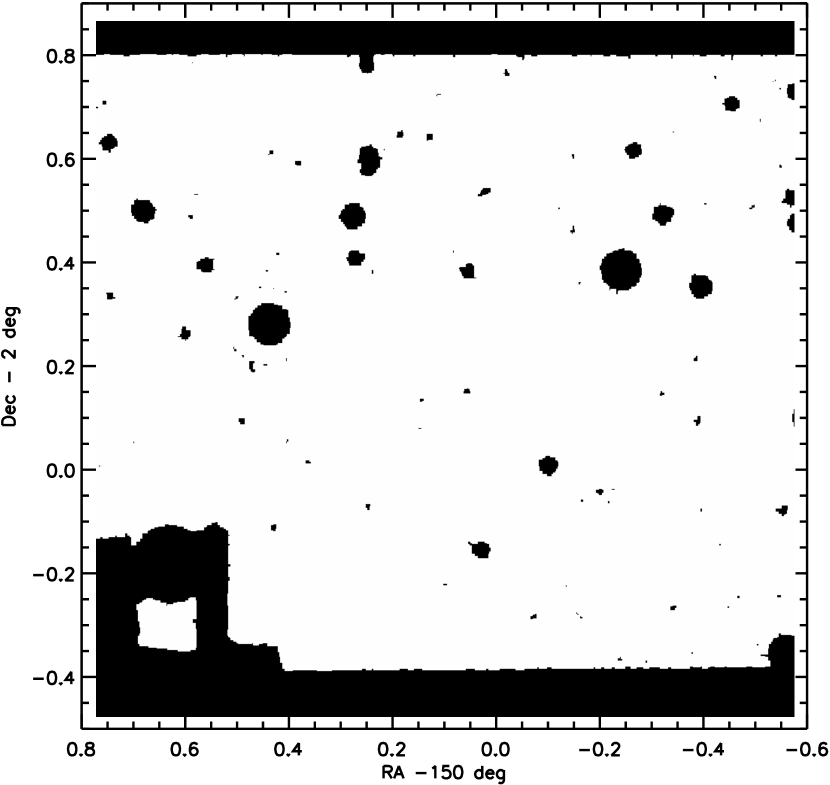
Figure 29: Masked areas around bright stars are shown in black (as generated from COSMOS I and B band masks). In these regions, accurate photometry is precluded and all galaxies in these regions are excluded from the LSS mapping and analysis. They appear as blank areas in the LSS maps at all redshifts.

References

- Arnouts et al. (2002) Arnouts, S., Moscardini, L., Vanzella, E., Colombi, S., Cristiani, S., Fontana, A., Giallongo, E., Matarrese, S., & Saracco, P. 2002, MNRAS, 329, 355
- Arnouts et al. (2005) Arnouts, S., Schiminovich, D., Ilbert, O., Tresse, L., Milliard, B., Treyer, M., Bardelli, S., Budavari, T., Wyder, T. K., Zucca, E., Le Fèvre, O., Martin, D. C., Vettolani, G., Adami, C., Arnaboldi, M., Barlow, T., Bianchi, L., Bolzonella, M., Bottini, D., Byun, Y.-I., Cappi, A., Charlot, S., Contini, T., Donas, J., Forster, K., Foucaud, S., Franzetti, P., Friedman, P. G., Garilli, B., Gavignaud, I., Guzzo, L., Heckman, T. M., Hoopes, C., Iovino, A., Jelinsky, P., Le Brun, V., Lee, Y.-W., Maccagni, D., Madore, B. F., Malina, R., Marano, B., Marinoni, C., McCracken, H. J., Mazure, A., Meneux, B., Merighi, R., Morrissey, P., Neff, S., Paltani, S., Pellò, R., Picat, J. P., Pollo, A., Pozzetti, L., Radovich, M., Rich, R. M., Scaramella, R., Scodeggio, M., Seibert, M., Siegmund, O., Small, T., Szalay, A. S., Welsh, B., Xu, C. K., Zamorani, G., & Zanichelli, A. 2005, ApJ, 619, L43
- Arnouts et al. (2007) Arnouts, S., Walcher, C. J., Le Fèvre, O., Zamorani, G., Ilbert, O., Le Brun, V., Pozzetti, L., Bardelli, S., Tresse, L., Zucca, E., Charlot, S., Lamareille, F., McCracken, H. J., Bolzonella, M., Iovino, A., Lonsdale, C., Polletta, M., Surace, J., Bottini, D., Garilli, B., Maccagni, D., Picat, J. P., Scaramella, R., Scodeggio, M., Vettolani, G., Zanichelli, A., Adami, C., Cappi, A., Ciliegi, P., Contini, T., de la Torre, S., Foucaud, S., Franzetti, P., Gavignaud, I., Guzzo, L., Marano, B., Marinoni, C., Mazure, A., Meneux, B., Merighi, R., Paltani, S., Pellò, R., Pollo, A., Radovich, M., Temporin, S., & Vergani, D. 2007, A&A, 476, 137
- Baldry et al. (2006) Baldry, I. K., Balogh, M. L., Bower, R. G., Glazebrook, K., Nichol, R. C., Bamford, S. P., & Budavari, T. 2006, MNRAS, 373, 469
- Balogh et al. (2004) Balogh, M., Eke, V., Miller, C., Lewis, I., Bower, R., Couch, W., Nichol, R., Bland-Hawthorn, J., Baldry, I. K., Baugh, C., Bridges, T., Cannon, R., Cole, S., Colless, M., Collins, C., Cross, N., Dalton, G., de Propris, R., Driver, S. P., Efstathiou, G., Ellis, R. S., Frenk, C. S., Glazebrook, K., Gomez, P., Gray, A., Hawkins, E., Jackson, C., Lahav, O., Lumsden, S., Maddox, S., Madgwick, D., Norberg, P., Peacock, J. A., Percival, W., Peterson, B. A., Sutherland, W., & Taylor, K. 2004, MNRAS, 348, 1355
- Bolzonella et al. (2010) Bolzonella, M., Kovač, K., Pozzetti, L., Zucca, E., Cucciati, O., Lilly, S. J., Peng, Y., Iovino, A., Zamorani, G., Vergani, D., Tasca, L. A. M., Lamareille, F., Oesch, P., Caputi, K., Kampczyk, P., Bardelli, S., Maier, C., Abbas, U., Knobel, C., Scodeggio, M., Carollo, C. M., Contini, T., Kneib, J.-P., Le Fèvre, O., Mainieri, V., Renzini, A., Bongiorno, A., Coppa, G., de la Torre, S., de Ravel, L., Franzetti, P., Garilli, B., Le Borgne, J.-F., Le Brun, V., Mignoli, M., Pelló, R., Perez-Montero, E., Ricciardelli, E., Silverman, J. D., Tanaka, M., Tresse, L., Bottini, D., Cappi, A., Cassata, P., Cimatti, A., Guzzo, L., Koekemoer, A. M., Leauthaud, A., Maccagni, D., Marinoni, C., McCracken, H. J., Memeo, P., Meneux, B., Porciani, C., Scaramella, R., Aussel, H., Capak, P., Halliday, C., Ilbert, O., Kartaltepe, J., Salvato, M., Sanders, D., Scarlata, C., Scoville, N., Taniguchi, Y., & Thompson, D. 2010, A&A, 524, A76
- Bouché et al. (2010) Bouché, N., Dekel, A., Genzel, R., Genel, S., Cresci, G., Förster Schreiber, N. M., Shapiro, K. L., Davies, R. I., & Tacconi, L. 2010, ApJ, 718, 1001
- Bruzual & Charlot (1993) Bruzual, A. G. & Charlot, S. 1993, ApJ, 405, 538
- Calzetti et al. (2000) Calzetti, D., Armus, L., Bohlin, R. C., Kinney, A. L., Koornneef, J., & Storchi-Bergmann, T. 2000, ApJ, 533, 682
- Capak (2009) Capak, P., e. a. 2009, ApJ, in preparation
- Capak (2013) —. 2013, ApJ, in preparation
- Capak et al. (2007) Capak, P., Abraham, R. G., Ellis, R. S., Mobasher, B., Scoville, N., Sheth, K., & Koekemoer, A. 2007, ApJS, 172, 284
- Cassata et al. (2007) Cassata, P., Guzzo, L., Franceschini, A., Scoville, N., Capak, P., Ellis, R. S., Koekemoer, A., McCracken, H. J., Mobasher, B., Renzini, A., Ricciardelli, E., Scodeggio, M., Taniguchi, Y., & Thompson, D. 2007, ApJS, 172, 270
- Chabrier (2003) Chabrier, G. 2003, PASP, 115, 763
- Coil et al. (2006) Coil, A. L., Gerke, B. F., Newman, J. A., Ma, C.-P., Yan, R., Cooper, M. C., Davis, M., Faber, S. M., Guhathakurta, P., & Koo, D. C. 2006, ApJ, 638, 668
- Cooper et al. (2006) Cooper, M. C., Newman, J. A., Croton, D. J., Weiner, B. J., Willmer, C. N. A., Gerke, B. F., Madgwick, D. S., Faber, S. M., Davis, M., Coil, A. L., Finkbeiner, D. P., Guhathakurta, P., & Koo, D. C. 2006, MNRAS, 370, 198
- Cooper et al. (2008) Cooper, M. C., Newman, J. A., Weiner, B. J., Yan, R., Willmer, C. N. A., Bundy, K., Coil, A. L., Conselice, C. J., Davis, M., Faber, S. M., Gerke, B. F., Guhathakurta, P., Koo, D. C., & Noeske, K. G. 2008, MNRAS, 383, 1058
- Croton et al. (2006) Croton, D. J., Springel, V., White, S. D. M., De Lucia, G., Frenk, C. S., Gao, L., Jenkins, A., Kauffmann, G., Navarro, J. F., & Yoshida, N. 2006, MNRAS, 365, 11
- Cucciati et al. (2010) Cucciati, O., Iovino, A., Kovač, K., Scodeggio, M., Lilly, S. J., Bolzonella, M., Bardelli, S., Vergani, D., Tasca, L. A. M., Zucca, E., Zamorani, G., Pozzetti, L., Knobel, C., Oesch, P., Lamareille, F., Caputi, K., Kampczyk, P., Tresse, L., Maier, C., Carollo, C. M., Contini, T., Kneib, J.-P., Le Fèvre, O., Mainieri, V., Renzini, A., Bongiorno, A., Coppa, G., de la Torre, S., de Ravel, L., Franzetti, P., Garilli, B., Le Borgne, J.-F., Le Brun, V., Mignoli, M., Pellò, R., Peng, Y., Perez-Montero, E., Ricciardelli, E., Silverman, J. D., Tanaka, M., Koekemoer, A. M., Scoville, N., Abbas, U., Bottini, D., Cappi, A., Cassata, P., Cimatti, A., Guzzo, L., Leauthaud, A., Maccagni, D., Marinoni, C., McCracken, H. J., Memeo, P., Meneux, B., Porciani, C., & Scaramella, R. 2010, A&A, 524, A2
- De Lucia & Blaizot (2007) De Lucia, G. & Blaizot, J. 2007, MNRAS, 375, 2
- Dressler et al. (1997) Dressler, A., Oemler, A. J., Couch, W. J., Smail, I., Ellis, R. S., Barger, A., Butcher, H., Poggianti, B. M., & Sharples, R. M. 1997, ApJ, 490, 577
- Ebeling & Wiedenmann (1993) Ebeling, H. & Wiedenmann, G. 1993, Phys. Rev. E, 47, 704
- Elbaz et al. (2007) Elbaz, D., Daddi, E., Le Borgne, D., Dickinson, M., Alexander, D. M., Chary, R., Starck, J., Brandt, W. N., Kitzbichler, M., MacDonald, E., Nonino, M., Popesso, P., Stern, D., & Vanzella, E. 2007, A&A, 468, 33
- Finoguenov et al. (2007) Finoguenov, A., Guzzo, L., Hasinger, G., Scoville, N. Z., Aussel, H., Böhringer, H., Brusa, M., Capak, P., Cappelluti, N., Comastri, A., Giodini, S., Griffiths, R. E., Impey, C., Koekemoer, A. M., Kneib, J.-P., Leauthaud, A., Le Fèvre, O., Lilly, S., Mainieri, V., Massey, R., McCracken, H. J., Mobasher, B., Murayama, T., Peacock, J. A., Sakelliou, I., Schinnerer, E., Silverman, J. D., Smolčić, V., Taniguchi, Y., Tasca, L., Taylor, J. E., Trump, J. R., & Zamorani, G. 2007, ApJS, 172, 182
- Gerke et al. (2005) Gerke, B. F., Newman, J. A., Davis, M., Marinoni, C., Yan, R., Coil, A. L., Conroy, C., Cooper, M. C., Faber, S. M., Finkbeiner, D. P., Guhathakurta, P., Kaiser, N., Koo, D. C., Phillips, A. C., Weiner, B. J., & Willmer, C. N. A. 2005, ApJ, 625, 6
- Gladders & Yee (2005) Gladders, M. D. & Yee, H. K. C. 2005, ApJS, 157, 1
- Gómez et al. (2003) Gómez, P. L., Nichol, R. C., Miller, C. J., Balogh, M. L., Goto, T., Zabludoff, A. I., Romer, A. K., Bernardi, M., Sheth, R., Hopkins, A. M., Castander, F. J., Connolly, A. J., Schneider, D. P., Brinkmann, J., Lamb, D. Q., SubbaRao, M., & York, D. G. 2003, ApJ, 584, 210
- Guo et al. (2011) Guo, Q., White, S., Boylan-Kolchin, M., De Lucia, G., Kauffmann, G., Lemson, G., Li, C., Springel, V., & Weinmann, S. 2011, MNRAS, 413, 101
- Guo & White (2009) Guo, Q. & White, S. D. M. 2009, ApJ, in preparation
- Guzzo et al. (2007) Guzzo, L., Cassata, P., Finoguenov, A., Massey, R., Scoville, N. Z., Capak, P., Ellis, R. S., Mobasher, B., Taniguchi, Y., Thompson, D., Ajiki, M., Aussel, H., Böhringer, H., Brusa, M., Calzetti, D., Comastri, A., Franceschini, A., Hasinger, G., Kasliwal, M. M., Kitzbichler, M. G., Kneib, J.-P., Koekemoer, A., Leauthaud, A., McCracken, H. J., Murayama, T., Nagao, T., Rhodes, J., Sanders, D. B., Sasaki, S., Shioya, Y., Tasca, L., & Taylor, J. E. 2007, ApJS, 172, 254
- Ideue et al. (2012) Ideue, Y., Taniguchi, Y., Nagao, T., Shioya, Y., Kajisawa, M., Trump, J. R., Vergani, D., Iovino, A., Koekemoer, A. M., Le Fèvre, O., Ilbert, O., & Scoville, N. Z. 2012, ApJ, 747, 42
- Ilbert et al. (2006) Ilbert, O., Arnouts, S., McCracken, H. J., Bolzonella, M., Bertin, E., Le Fèvre, O., Mellier, Y., Zamorani, G., Pellò, R., Iovino, A., Tresse, L., Le Brun, V., Bottini, D., Garilli, B., Maccagni, D., Picat, J. P., Scaramella, R., Scodeggio, M., Vettolani, G., Zanichelli, A., Adami, C., Bardelli, S., Cappi, A., Charlot, S., Ciliegi, P., Contini, T., Cucciati, O., Foucaud, S., Franzetti, P., Gavignaud, I., Guzzo, L., Marano, B., Marinoni, C., Mazure, A., Meneux, B., Merighi, R., Paltani, S., Pollo, A., Pozzetti, L., Radovich, M., Zucca, E., Bondi, M., Bongiorno, A., Busarello, G., de La Torre, S., Gregorini, L., Lamareille, F., Mathez, G., Merluzzi, P., Ripepi, V., Rizzo, D., & Vergani, D. 2006, A&A, 457, 841
- Ilbert et al. (2009) Ilbert, O., Capak, P., Salvato, M., Aussel, H., McCracken, H. J., Sanders, D. B., Scoville, N., Kartaltepe, J., Arnouts, S., Floc’h, E. L., Mobasher, B., Taniguchi, Y., Lamareille, F., Leauthaud, A., Sasaki, S., Thompson, D., Zamojski, M., Zamorani, G., Bardelli, S., Bolzonella, M., Bongiorno, A., Brusa, M., Caputi, K. I., Carollo, C. M., Contini, T., Cook, R., Coppa, G., Cucciati, O., de la Torre, S., de Ravel, L., Franzetti, P., Garilli, B., Hasinger, G., Iovino, A., Kampczyk, P., Kneib, J.-P., Knobel, C., Kovac, K., LeBorgne, J. F., LeBrun, V., Fèvre, O. L., Lilly, S., Looper, D., Maier, C., Mainieri, V., Mellier, Y., Mignoli, M., Murayama, T., Pellò, R., Peng, Y., Pérez-Montero, E., Renzini, A., Ricciardelli, E., Schiminovich, D., Scodeggio, M., Shioya, Y., Silverman, J., Surace, J., Tanaka, M., Tasca, L., Tresse, L., Vergani, D., & Zucca, E. 2009, ApJ, 690, 1236
- Ilbert et al. (2013) Ilbert, O., McCracken, H. J., Le Fevre, O., Capak, P., Dunlop, J., Arnouts, S., Aussel, H., Caputi, K., Comparat, J., Guo, Q., Hudelot, P., Kartaltepe, J., Kneib, J. P., Krogager, J. K., Le Floc’h, E., Lilly, S., Mellier, Y., Milvang-Jensen, B., Moutard, T., Onodera, M., Renzini, M. A., Richard, J., Salvato, M., Sanders, D. B., Scoville, N., Silverman, J., Taniguchi, Y., Tasca, L., Thomas, R., Toft, S., Tresse, L., Vergani, D., Wolk, M., & Zirm, A. 2013, ArXiv e-prints
- Ilbert et al. (2010) Ilbert, O., Salvato, M., Le Floc’h, E., Aussel, H., Capak, P., McCracken, H. J., Mobasher, B., Kartaltepe, J., Scoville, N., Sanders, D. B., Arnouts, S., Bundy, K., Cassata, P., Kneib, J.-P., Koekemoer, A., Le Fèvre, O., Lilly, S., Surace, J., Taniguchi, Y., Tasca, L., Thompson, D., Tresse, L., Zamojski, M., Zamorani, G., & Zucca, E. 2010, ApJ, 709, 644
- Iovino et al. (2010) Iovino, A., Cucciati, O., Scodeggio, M., Knobel, C., Kovač, K., Lilly, S., Bolzonella, M., Tasca, L. A. M., Zamorani, G., Zucca, E., Caputi, K., Pozzetti, L., Oesch, P., Lamareille, F., Halliday, C., Bardelli, S., Finoguenov, A., Guzzo, L., Kampczyk, P., Maier, C., Tanaka, M., Vergani, D., Carollo, C. M., Contini, T., Kneib, J.-P., Le Fèvre, O., Mainieri, V., Renzini, A., Bongiorno, A., Coppa, G., de la Torre, S., de Ravel, L., Franzetti, P., Garilli, B., Le Borgne, J.-F., Le Brun, V., Mignoli, M., Pellò, R., Peng, Y., Perez-Montero, E., Ricciardelli, E., Silverman, J. D., Tresse, L., Abbas, U., Bottini, D., Cappi, A., Cassata, P., Cimatti, A., Koekemoer, A. M., Leauthaud, A., Maccagni, D., Marinoni, C., McCracken, H. J., Memeo, P., Meneux, B., Porciani, C., Scaramella, R., Schiminovich, D., & Scoville, N. 2010, A&A, 509, A40
- Karim et al. (2011) Karim, A., Schinnerer, E., Martínez-Sansigre, A., Sargent, M. T., van der Wel, A., Rix, H.-W., Ilbert, O., Smolčić, V., Carilli, C., Pannella, M., Koekemoer, A. M., Bell, E. F., & Salvato, M. 2011, ApJ, 730, 61
- Kauffmann et al. (2004) Kauffmann, G., White, S. D. M., Heckman, T. M., Ménard, B., Brinchmann, J., Charlot, S., Tremonti, C., & Brinkmann, J. 2004, MNRAS, 353, 713
- Kennicutt (1998) Kennicutt, Jr., R. C. 1998, ARA&A, 36, 189
- Kitzbichler & White (2007) Kitzbichler, M. G. & White, S. D. M. 2007, MNRAS, 376, 2
- Knobel et al. (2012) Knobel, C., Lilly, S. J., Iovino, A., Kovač, K., Bschorr, T. J., Presotto, V., Oesch, P. A., Kampczyk, P., Carollo, C. M., Contini, T., Kneib, J.-P., Le Fevre, O., Mainieri, V., Renzini, A., Scodeggio, M., Zamorani, G., Bardelli, S., Bolzonella, M., Bongiorno, A., Caputi, K., Cucciati, O., de la Torre, S., de Ravel, L., Franzetti, P., Garilli, B., Lamareille, F., Le Borgne, J.-F., Le Brun, V., Maier, C., Mignoli, M., Pello, R., Peng, Y., Perez Montero, E., Silverman, J., Tanaka, M., Tasca, L., Tresse, L., Vergani, D., Zucca, E., Barnes, L., Bordoloi, R., Cappi, A., Cimatti, A., Coppa, G., Koekemoer, A. M., López-Sanjuan, C., McCracken, H. J., Moresco, M., Nair, P., Pozzetti, L., & Welikala, N. 2012, ApJ, 753, 121
- Knobel et al. (2009) Knobel, C., Lilly, S. J., Iovino, A., Porciani, C., Kovač, K., Cucciati, O., Finoguenov, A., Kitzbichler, M. G., Carollo, C. M., Contini, T., Kneib, J.-P., Le Fèvre, O., Mainieri, V., Renzini, A., Scodeggio, M., Zamorani, G., Bardelli, S., Bolzonella, M., Bongiorno, A., Caputi, K., Coppa, G., de la Torre, S., de Ravel, L., Franzetti, P., Garilli, B., Kampczyk, P., Lamareille, F., Le Borgne, J.-F., Le Brun, V., Maier, C., Mignoli, M., Pello, R., Peng, Y., Perez Montero, E., Ricciardelli, E., Silverman, J. D., Tanaka, M., Tasca, L., Tresse, L., Vergani, D., Zucca, E., Abbas, U., Bottini, D., Cappi, A., Cassata, P., Cimatti, A., Fumana, M., Guzzo, L., Koekemoer, A. M., Leauthaud, A., Maccagni, D., Marinoni, C., McCracken, H. J., Memeo, P., Meneux, B., Oesch, P., Pozzetti, L., & Scaramella, R. 2009, ApJ, 697, 1842
- Kovač et al. (2010) Kovač, K., Lilly, S. J., Cucciati, O., Porciani, C., Iovino, A., Zamorani, G., Oesch, P., Bolzonella, M., Knobel, C., Finoguenov, A., Peng, Y., Carollo, C. M., Pozzetti, L., Caputi, K., Silverman, J. D., Tasca, L. A. M., Scodeggio, M., Vergani, D., Scoville, N. Z., Capak, P., Contini, T., Kneib, J.-P., Le Fèvre, O., Mainieri, V., Renzini, A., Bardelli, S., Bongiorno, A., Coppa, G., de la Torre, S., de Ravel, L., Franzetti, P., Garilli, B., Guzzo, L., Kampczyk, P., Lamareille, F., Le Borgne, J.-F., Le Brun, V., Maier, C., Mignoli, M., Pello, R., Perez Montero, E., Ricciardelli, E., Tanaka, M., Tresse, L., Zucca, E., Abbas, U., Bottini, D., Cappi, A., Cassata, P., Cimatti, A., Fumana, M., Koekemoer, A. M., Maccagni, D., Marinoni, C., McCracken, H. J., Memeo, P., Meneux, B., & Scaramella, R. 2010, ApJ, 708, 505
- Le Fèvre et al. (2005) Le Fèvre, O., Guzzo, L., Meneux, B., Pollo, A., Cappi, A., Colombi, S., Iovino, A., Marinoni, C., McCracken, H. J., Scaramella, R., Bottini, D., Garilli, B., Le Brun, V., Maccagni, D., Picat, J. P., Scodeggio, M., Tresse, L., Vettolani, G., Zanichelli, A., Adami, C., Arnaboldi, M., Arnouts, S., Bardelli, S., Blaizot, J., Bolzonella, M., Charlot, S., Ciliegi, P., Contini, T., Foucaud, S., Franzetti, P., Gavignaud, I., Ilbert, O., Marano, B., Mathez, G., Mazure, A., Merighi, R., Paltani, S., Pellò, R., Pozzetti, L., Radovich, M., Zamorani, G., Zucca, E., Bondi, M., Bongiorno, A., Busarello, G., Lamareille, F., Mellier, Y., Merluzzi, P., Ripepi, V., & Rizzo, D. 2005, A&A, 439, 877
- Lee et al. (2010) Lee, N., Le Floc’h, E., Sanders, D. B., Frayer, D. T., Arnouts, S., Ilbert, O., Aussel, H., Salvato, M., Scoville, N. Z., & Kartaltepe, J. S. 2010, ApJ, 717, 175
- Lilly et al. (2007) Lilly, S. J., Le Fèvre, O., Renzini, A., Zamorani, G., Scodeggio, M., Contini, T., Carollo, C. M., Hasinger, G., Kneib, J.-P., Iovino, A., Le Brun, V., Maier, C., Mainieri, V., Mignoli, M., Silverman, J., Tasca, L. A. M., Bolzonella, M., Bongiorno, A., Bottini, D., Capak, P., Caputi, K., Cimatti, A., Cucciati, O., Daddi, E., Feldmann, R., Franzetti, P., Garilli, B., Guzzo, L., Ilbert, O., Kampczyk, P., Kovac, K., Lamareille, F., Leauthaud, A., Borgne, J.-F. L., McCracken, H. J., Marinoni, C., Pello, R., Ricciardelli, E., Scarlata, C., Vergani, D., Sanders, D. B., Schinnerer, E., Scoville, N., Taniguchi, Y., Arnouts, S., Aussel, H., Bardelli, S., Brusa, M., Cappi, A., Ciliegi, P., Finoguenov, A., Foucaud, S., Franceschini, R., Halliday, C., Impey, C., Knobel, C., Koekemoer, A., Kurk, J., Maccagni, D., Maddox, S., Marano, B., Marconi, G., Meneux, B., Mobasher, B., Moreau, C., Peacock, J. A., Porciani, C., Pozzetti, L., Scaramella, R., Schiminovich, D., Shopbell, P., Smail, I., Thompson, D., Tresse, L., Vettolani, G., Zanichelli, A., & Zucca, E. 2007, ApJS, 172, 70
- Marinoni et al. (2002) Marinoni, C., Davis, M., Newman, J. A., & Coil, A. L. 2002, ApJ, 580, 122
- Massey et al. (2007) Massey, R., Rhodes, J., Ellis, R., Scoville, N., Leauthaud, A., Finoguenov, A., Capak, P., Bacon, D., Aussel, H., Kneib, J.-P., Koekemoer, A., McCracken, H., Mobasher, B., Pires, S., Refregier, A., Sasaki, S., Starck, J.-L., Taniguchi, Y., Taylor, A., & Taylor, J. 2007, Nature, 445, 286
- McCracken et al. (2010) McCracken, H. J., Capak, P., Salvato, M., Aussel, H., Thompson, D., Daddi, E., Sanders, D. B., Kneib, J.-P., Willott, C. J., Mancini, C., Renzini, A., Cook, R., Le Fèvre, O., Ilbert, O., Kartaltepe, J., Koekemoer, A. M., Mellier, Y., Murayama, T., Scoville, N. Z., Shioya, Y., & Tanaguchi, Y. 2010, ApJ, 708, 202
- McCracken et al. (2012) McCracken, H. J., Milvang-Jensen, B., Dunlop, J., Franx, M., Fynbo, J. P. U., Le Fèvre, O., Holt, J., Caputi, K. I., Goranova, Y., Buitrago, F., Emerson, J., Freudling, W., Hudelot, P., López-Sanjuan, C., Magnard, F., Mellier, Y., Møller, P., Nilsson, K. K., Sutherland, W., Tasca, L., & Zabl, J. 2012, ArXiv e-prints
- McGee et al. (2009) McGee, S. L., Balogh, M. L., Bower, R. G., Font, A. S., & McCarthy, I. G. 2009, MNRAS, 400, 937
- Meneux et al. (2006) Meneux, B., Le Fèvre, O., Guzzo, L., Pollo, A., Cappi, A., Ilbert, O., Iovino, A., Marinoni, C., McCracken, H. J., Bottini, D., Garilli, B., Le Brun, V., Maccagni, D., Picat, J. P., Scaramella, R., Scodeggio, M., Tresse, L., Vettolani, G., Zanichelli, A., Adami, C., Arnouts, S., Arnaboldi, M., Bardelli, S., Bolzonella, M., Charlot, S., Ciliegi, P., Contini, T., Foucaud, S., Franzetti, P., Gavignaud, I., Marano, B., Mazure, A., Merighi, R., Paltani, S., Pellò, R., Pozzetti, L., Radovich, M., Zamorani, G., Zucca, E., Bondi, M., Bongiorno, A., Busarello, G., Cucciati, O., Gregorini, L., Lamareille, F., Mathez, G., Mellier, Y., Merluzzi, P., Ripepi, V., & Rizzo, D. 2006, A&A, 452, 387
- Neistein & Dekel (2008) Neistein, E. & Dekel, A. 2008, MNRAS, 388, 1792
- Onodera et al. (2012) Onodera, M., Renzini, A., Carollo, M., Cappellari, M., Mancini, C., Strazzullo, V., Daddi, E., Arimoto, N., Gobat, R., Yamada, Y., McCracken, H. J., Ilbert, O., Capak, P., Cimatti, A., Giavalisco, M., Koekemoer, A. M., Kong, X., Lilly, S., Motohara, K., Ohta, K., Sanders, D. B., Scoville, N., Tamura, N., & Taniguchi, Y. 2012, ApJ, 755, 26
- Patel et al. (2009) Patel, S. G., Holden, B. P., Kelson, D. D., Illingworth, G. D., & Franx, M. 2009, ApJ, 705, L67
- Peng et al. (2010) Peng, Y., Lilly, S. J., Kovač, K., Bolzonella, M., Pozzetti, L., Renzini, A., Zamorani, G., Ilbert, O., Knobel, C., Iovino, A., Maier, C., Cucciati, O., Tasca, L., Carollo, C. M., Silverman, J., Kampczyk, P., de Ravel, L., Sanders, D., Scoville, N., Contini, T., Mainieri, V., Scodeggio, M., Kneib, J., Le Fèvre, O., Bardelli, S., Bongiorno, A., Caputi, K., Coppa, G., de la Torre, S., Franzetti, P., Garilli, B., Lamareille, F., Le Borgne, J., Le Brun, V., Mignoli, M., Perez Montero, E., Pello, R., Ricciardelli, E., Tanaka, M., Tresse, L., Vergani, D., Welikala, N., Zucca, E., Oesch, P., Abbas, U., Barnes, L., Bordoloi, R., Bottini, D., Cappi, A., Cassata, P., Cimatti, A., Fumana, M., Hasinger, G., Koekemoer, A., Leauthaud, A., Maccagni, D., Marinoni, C., McCracken, H., Memeo, P., Meneux, B., Nair, P., Porciani, C., Presotto, V., & Scaramella, R. 2010, ApJ, 721, 193
- Postman et al. (1996) Postman, M., Lubin, L. M., Gunn, J. E., Oke, J. B., Hoessel, J. G., Schneider, D. P., & Christensen, J. A. 1996, AJ, 111, 615
- Prevot et al. (1984) Prevot, M. L., Lequeux, J., Prevot, L., Maurice, E., & Rocca-Volmerange, B. 1984, A&A, 132, 389
- Sanders et al. (2007) Sanders, D. B., Salvato, M., Aussel, H., Ilbert, O., Scoville, N., Surace, J. A., Frayer, D. T., Sheth, K., Helou, G., Brooke, T., Bhattacharya, B., Yan, L., Kartaltepe, J. S., Barnes, J. E., Blain, A. W., Calzetti, D., Capak, P., Carilli, C., Carollo, C. M., Comastri, A., Daddi, E., Ellis, R. S., Elvis, M., Fall, S. M., Franceschini, A., Giavalisco, M., Hasinger, G., Impey, C., Koekemoer, A., Le Fèvre, O., Lilly, S., Liu, M. C., McCracken, H. J., Mobasher, B., Renzini, A., Rich, M., Schinnerer, E., Shopbell, P. L., Taniguchi, Y., Thompson, D. J., Urry, C. M., & Williams, J. P. 2007, ApJS, 172, 86
- Schiminovich et al. (2005) Schiminovich, D., Ilbert, O., Arnouts, S., Milliard, B., Tresse, L., Le Fèvre, O., Treyer, M., Wyder, T. K., Budavári, T., Zucca, E., Zamorani, G., Martin, D. C., Adami, C., Arnaboldi, M., Bardelli, S., Barlow, T., Bianchi, L., Bolzonella, M., Bottini, D., Byun, Y.-I., Cappi, A., Contini, T., Charlot, S., Donas, J., Forster, K., Foucaud, S., Franzetti, P., Friedman, P. G., Garilli, B., Gavignaud, I., Guzzo, L., Heckman, T. M., Hoopes, C., Iovino, A., Jelinsky, P., Le Brun, V., Lee, Y.-W., Maccagni, D., Madore, B. F., Malina, R., Marano, B., Marinoni, C., McCracken, H. J., Mazure, A., Meneux, B., Morrissey, P., Neff, S., Paltani, S., Pellò, R., Picat, J. P., Pollo, A., Pozzetti, L., Radovich, M., Rich, R. M., Scaramella, R., Scodeggio, M., Seibert, M., Siegmund, O., Small, T., Szalay, A. S., Vettolani, G., Welsh, B., Xu, C. K., & Zanichelli, A. 2005, ApJ, 619, L47
- Schuecker & Boehringer (1998) Schuecker, P. & Boehringer, H. 1998, A&A, 339, 315
- Scoville et al. (2007a) Scoville, N., Abraham, R. G., Aussel, H., Barnes, J. E., Benson, A., Blain, A. W., Calzetti, D., Comastri, A., Capak, P., Carilli, C., Carlstrom, J. E., Carollo, C. M., Colbert, J., Daddi, E., Ellis, R. S., Elvis, M., Ewald, S. P., Fall, M., Franceschini, A., Giavalisco, M., Green, W., Griffiths, R. E., Guzzo, L., Hasinger, G., Impey, C., Kneib, J.-P., Koda, J., Koekemoer, A., Lefevre, O., Lilly, S., Liu, C. T., McCracken, H. J., Massey, R., Mellier, Y., Miyazaki, S., Mobasher, B., Mould, J., Norman, C., Refregier, A., Renzini, A., Rhodes, J., Rich, M., Sanders, D. B., Schiminovich, D., Schinnerer, E., Scodeggio, M., Sheth, K., Shopbell, P. L., Taniguchi, Y., Tyson, N. D., Urry, C. M., Van Waerbeke, L., Vettolani, P., White, S. D. M., & Yan, L. 2007a, ApJS, 172, 38
- Scoville et al. (2007b) Scoville, N., Aussel, H., Benson, A., Blain, A., Calzetti, D., Capak, P., Ellis, R. S., El-Zant, A., Finoguenov, A., Giavalisco, M., Guzzo, L., Hasinger, G., Koda, J., Le Fèvre, O., Massey, R., McCracken, H. J., Mobasher, B., Renzini, A., Rhodes, J., Salvato, M., Sanders, D. B., Sasaki, S. S., Schinnerer, E., Sheth, K., Shopbell, P. L., Taniguchi, Y., Taylor, J. E., & Thompson, D. J. 2007b, ApJS, 172, 150
- Scoville & Li (2011) Scoville, N. & Li, G. 2011, in Astronomical Society of the Pacific Conference Series, Vol. 440, UP2010: Have Observations Revealed a Variable Upper End of the Initial Mass Function?, ed. M. Treyer, T. Wyder, J. Neill, M. Seibert, & J. Lee, 317
- Smith et al. (2005) Smith, G. P., Treu, T., Ellis, R. S., Moran, S. M., & Dressler, A. 2005, ApJ, 620, 78
- Spergel et al. (2007) Spergel, D. N., Bean, R., Doré, O., Nolta, M. R., Bennett, C. L., Dunkley, J., Hinshaw, G., Jarosik, N., Komatsu, E., Page, L., Peiris, H. V., Verde, L., Halpern, M., Hill, R. S., Kogut, A., Limon, M., Meyer, S. S., Odegard, N., Tucker, G. S., Weiland, J. L., Wollack, E., & Wright, E. L. 2007, ApJS, 170, 377
- Springel et al. (2005) Springel, V., White, S. D. M., Jenkins, A., Frenk, C. S., Yoshida, N., Gao, L., Navarro, J., Thacker, R., Croton, D., Helly, J., Peacock, J. A., Cole, S., Thomas, P., Couchman, H., Evrard, A., Colberg, J., & Pearce, F. 2005, Nature, 435, 629
- Taniguchi et al. (2007) Taniguchi, Y., Scoville, N., Murayama, T., Sanders, D. B., Mobasher, B., Aussel, H., Capak, P., Ajiki, M., Miyazaki, S., Komiyama, Y., Shioya, Y., Nagao, T., Sasaki, S. S., Koda, J., Carilli, C., Giavalisco, M., Guzzo, L., Hasinger, G., Impey, C., LeFevre, O., Lilly, S., Renzini, A., Rich, M., Schinnerer, E., Shopbell, P., Kaifu, N., Karoji, H., Arimoto, N., Okamura, S., & Ohta, K. 2007, ApJS, 172, 9
- van de Weygaert (1994) van de Weygaert, R. 1994, A&A, 283, 361
- Wang et al. (2008) Wang, J., De Lucia, G., Kitzbichler, M. G., & White, S. D. M. 2008, MNRAS, 384, 1301
- Young & Scoville (1991) Young, J. S. & Scoville, N. Z. 1991, ARA&A, 29, 581
- Zamojski et al. (2007) Zamojski, M. A., Schiminovich, D., Rich, R. M., Mobasher, B., Koekemoer, A. M., Capak, P., Taniguchi, Y., Sasaki, S. S., McCracken, H. J., Mellier, Y., Bertin, E., Aussel, H., Sanders, D. B., Le Fèvre, O., Ilbert, O., Salvato, M., Thompson, D. J., Kartaltepe, J. S., Scoville, N., Barlow, T. A., Forster, K., Friedman, P. G., Martin, D. C., Morrissey, P., Neff, S. G., Seibert, M., Small, T., Wyder, T. K., Bianchi, L., Donas, J., Heckman, T. M., Lee, Y.-W., Madore, B. F., Milliard, B., Szalay, A. S., Welsh, B. Y., & Yi, S. K. 2007, ApJS, 172, 468