Renewal processes based on generalized Mittag–Leffler waiting times

Abstract

The fractional Poisson process has recently attracted experts from several fields of study. Its natural generalization of the ordinary Poisson process made the model more appealing for real-world applications. In this paper, we generalized the standard and fractional Poisson processes through the waiting time distribution, and showed their relations to an integral operator with a generalized Mittag–Leffler function in the kernel. The waiting times of the proposed renewal processes have the generalized Mittag–Leffler and stretched-squashed Mittag–Leffler distributions. Note that the generalizations naturally provide greater flexibility in modeling real-life renewal processes. Algorithms to simulate sample paths and to estimate the model parameters are derived. Note also that these procedures are necessary to make these models more usable in practice. State probabilities and other qualitative or quantitative features of the models are also discussed.

Keywords: Fractional Poisson process, generalized Mittag–Leffler distribution, renewal processes, Prabhakar operator.

1 Introduction

The fractional Poisson process [1, 2, 3, 4, 5, 6, 7, 8, 9, 10, 11, 12, 13] gained popularity in many areas of research as it naturally generalizes the standard or classical Poisson process. Recall that the inter-event time density function of the fractional Poisson process $N^{\nu}(t)$, $t\geq 0$, $\nu\in(0,1]$, was originally derived in Repin and Saichev [14] (known to date) and has the following integral form:

$$f^{\nu}(t)=\frac{1}{t}\int\limits_{0}^{\infty}e^{-x}\phi_{\nu}(\lambda t/x)\,\mathrm{d}x,\qquad\nu\in(0,1],\>t>0,\lambda>0,$$ (1.1)

where

$$\phi_{\nu}(\xi)=\frac{\sin(\nu\pi)}{\pi[\xi^{\nu}+\xi^{-\nu}+2\cos(\nu\pi)]}.$$ (1.2)

The preceding density function suggests that the tail distribution of the waiting time is of the form

$$\Pr\,(T^{\nu}>t)=E_{\nu}(-\lambda t^{\nu}),$$ (1.3)

where

$$E_{\beta}(z)=\sum\limits_{n=0}^{\infty}\frac{z^{n}}{\Gamma(\beta n+1)},\qquad\>z\in\mathbb{C},\>\beta\in\mathbb{C},\Re(\beta)>0,$$ (1.4)

is the Mittag–Leffler function. Note that the Mittag–Leffler density has been widely used to describe distributions appearing in anomalous diffusion, finance and economics, transport of charge carriers in semiconductors, and light propagation through random media (see, e.g., [15, 16]). In view of equations (1.3) and (1.4), the interarrival time density for the fractional Poisson process directly follows as

$$f^{\nu}(t)=\lambda t^{\nu-1}E_{\nu,\,\nu}(-\lambda t^{\nu}),\qquad t>0,$$ (1.5)

where

$$E_{\beta,\gamma}(z)=\sum_{r=0}^{\infty}\frac{z^{r}}{\Gamma(\beta r+\gamma)},\qquad z\in\mathbb{C},\>\beta,\gamma\in\mathbb{C},\>\Re(\beta)>0$$ (1.6)

is the two-parameter Mittag–Leffler function. The $q$th fractional moment [17] of the random interarrival time is

$$\mathbb{E}\left[T^{\nu}\right]^{q}=\frac{\pi\Gamma(1+q)}{\lambda^{q}\Gamma(q/\nu)\sin(\pi q/\nu)\Gamma(1-q)},\qquad 0<q<\nu.$$ (1.7)

In addition, the above information automatically gives the probability density function

$$f_{m}^{\nu}(t)=\lambda^{m}\frac{t^{\nu m-1}}{(m-1)!}E_{\nu,\nu}^{(m-1)}\big{(}-\lambda t^{\nu}\big{)},$$ (1.8)

of the $m$-th arrival time because its Laplace transform,

$$\textsf{L}\big{\{}f_{m}^{\nu}(t)\big{\}}(s)=\int_{0}^{\infty}e^{-st}f_{m}^{\nu}(t)\,\mathrm{d}t=\frac{\lambda^{m}}{(\lambda+s^{\nu})^{m}},$$ (1.9)

where $E_{\nu,\nu}^{(k)}(-\lambda t^{\nu})$ is the $k$th derivative of $E_{\nu,\nu}(z)$ evaluated at $z=-\lambda t^{\nu}$. As $\nu\to 1$, the above distribution converges to the classical Erlang distribution.

In another approach to the study the fractional Poisson process, Laskin [1] used the fractional Kolmogorov–Feller-type differential equation system to characterize the one-dimensional state probability distributions as (see Laskin [1, formula (25)] and Beghin and Orsingher [5, formula (2.5)])

$$p_{k}^{\nu}(t)=\Pr\{N^{\nu}(t)=k\}=\frac{(\lambda t^{\nu})^{k}}{k!}\sum_{r=0}^{\infty}\frac{(r+k)!}{r!}\frac{(-\lambda t^{\nu})^{r}}{\Gamma(\nu(r+k)+1)},\qquad k\geq 0,\>t\geq 0.$$ (1.10)

One can also show [1] that the moment generating function (MGF) of the fractional Poisson process is

$$M_{\nu}(s,t) =E_{\nu}\left[\lambda(e^{-s}-1)t^{\nu}\right]=\sum_{r=0}^{\infty}\frac{\left[\lambda t^{\nu}\left(e^{-s}-1\right)\right]^{r}}{\Gamma(\nu r+1)},$$ (1.11)

which permits calculation (see Table 1) of the moments. A summary of the characteristics of the classical and fractional Poisson processes is shown in Table 1 below.

	Poisson process $(\nu=1)$	Fractional Poisson Process $(\nu<1)$
$\Pr(T^{\nu}>t)$	$e^{-\lambda t}$	$E_{\nu}(-\lambda t^{\nu})$
$f^{\nu}(t)$	$\lambda e^{-\lambda t}$	$\lambda t^{\nu-1}E_{\nu,\,\nu}(-\lambda t^{\nu})$
$p_{k}^{\nu}(t)$	$\frac{(\lambda t)^{k}}{k!}e^{-\lambda t}$	$\frac{(\lambda t^{\nu})^{k}}{k!}\sum_{r=0}^{\infty}\frac{(r+k)!}{r!}\frac{(-\lambda t^{\nu})^{r}}{\Gamma(\nu(r+k)+1)}$
Mean	$\lambda t$	$\lambda t^{\nu}/\Gamma(\nu+1)$
Variance	$\lambda t$	$\frac{\lambda t^{\nu}}{\Gamma(\nu+1)}+(\lambda t^{\nu})^{2}\left[\frac{1}{\nu\Gamma(2\nu)}-\frac{1}{\Gamma^{2}(\nu+1)}\right]$
$k$th moment	$(-1)^{k}\frac{\partial^{k}}{\partial s^{k}}\exp\left[\lambda(e^{-s}-1)t\right]\big{|}_{s=0}$	$\left(-1\right)^{k}\frac{\partial^{k}}{\partial s^{k}}E_{\nu}\left[\lambda(e^{-s}-1)t^{\nu}\right]\big{|}_{s=0}$

Table 1: Properties of fractional Poisson process compared with those of the standard Poisson process.

In this paper, we generalize the standard and fractional Poisson processes through their waiting time distributions. In particular, we propose two renewal processes that have waiting times that are generalized Mittag–Leffler and stretched-squashed Mittag–Leffler distributed. These generalizations naturally provide more flexibility in capturing real-world renewal processes. Algorithms to simulate sample paths and estimate the model parameters are derived and tested. State probabilities and other qualitative or quantitative features of the models are also discussed.

The rest of the paper is organized as follows. In Section 2, a renewal process with generalized Mittag–Leffler distributed waiting times is presented. Procedures to generate sample paths and to estimate parameters are also derived. In Section 3, another generalization based on stretching and squashing the Mittag–Leffler distributed inter-event times is developed. Methods to simulate sample trajectories and to estimate parameters are also showcased. More discussions are provided in Section 4. Finally, computational test results are shown in the appendix.

2 Generalization I

We consider the generalized Mittag–Leffler distribution (see e.g. Pillai [18]) built from the generalized Mittag–Leffler function [19, 20]. Let $T^{\nu,\delta}$ be a generalized Mittag–Leffler distributed random variable. Then the probability density function is

$$f^{\nu,\delta}(t)=\lambda^{\delta}t^{\delta\nu-1}E_{\nu,\delta\nu}^{\delta}(-\lambda t^{\nu}),\qquad t>0,\>\lambda>0,\>\nu\in(0,1],\>\delta\in\mathbb{R},$$ (2.1)

where

$$E_{\beta,\gamma}^{\xi}(z)=\sum_{r=0}^{\infty}\frac{(\xi)_{r}}{r!\Gamma(\beta r+\gamma)}z^{r},\quad\beta,\gamma,\xi,z\in\mathbb{C},\>\Re(\beta)>0$$ (2.2)

is the generalized Mittag–Leffler function (see Figure 1). The Pochhammer symbol $(\xi)_{r}$ can be written also as $(\xi)_{r}=\xi(\xi+1)\dots(\xi+r-1)$, $\xi\neq 0$. When $\delta\nu<1$ the function (2.1) has an asymptote at $t=0$, while in the particular case $\delta\nu=1$

$$\left.f^{\nu,\delta}(t)\right|_{t=0}=\left.\lambda^{1/\nu}E_{\nu,1}^{1/\nu}(-\lambda t^{\nu})\right|_{t=0}=\lambda^{1/\nu}.$$ (2.3)

The Laplace transform of (2.1) reads

$$\textsf{L}\big{\{}\lambda^{\delta}t^{\delta\nu-1}E_{\nu,\delta\nu}^{\delta}(-\lambda t^{\nu})\big{\}}(s)=\frac{\lambda^{\delta}}{(s^{\nu}+\lambda)^{\delta}}$$ (2.4)

(see Mathai and Haubold [21], formula (2.3.24), page 95). Below are the plots of the generalized Mittag–Leffler densities.

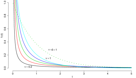
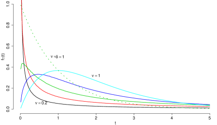
Figure 1: The generalized Mittag–Leffler density plots (see (2.1)) for parameter values $(\delta,\lambda)=(0.5,1)$ (top) and $(\delta,\lambda)=(2,1)$ (bottom) where $\nu$ goes from 0.2 to 1 with step size of 0.2.

Now, consider $m$ i.i.d. random waiting times $\mathcal{T}_{i}$, $i=1,\dots,m$ of a renewal point process, here denoted as $N^{\nu,\delta}(t)$, $t\geq 0$, which are distributed as in (2.1). Furthermore, denote $T_{m}^{\nu,\delta}=\mathcal{T}_{1}+\dots+\mathcal{T}_{m}$ as the waiting time of the $m$th renewal event and $T_{0}^{\nu,\delta}=0$. Then

$$\mathbb{E}e^{-sT_{m}^{\nu,\delta}}=\left(\mathbb{E}e^{-s\mathcal{T}_{i}}\right)^{m}=\frac{\lambda^{\delta m}}{(s^{\nu}+\lambda)^{\delta m}}.$$ (2.5)

By formula (2.3.24) of Mathai and Haubold [21] we have

$$\Pr\{T_{m}^{\nu,\delta}\in\mathrm{d}t\}/\mathrm{d}t=\lambda^{\delta m}t^{\nu\delta m-1}E_{\nu,\nu\delta m}^{\delta m}(-\lambda t^{\nu}),\qquad t>0,\>\lambda>0.$$ (2.6)

It is rather immediate now to obtain the state probabilities $p_{k}^{\nu,\delta}(t)=\Pr\{N^{\nu,\delta}(t)=k\}$, $k\geq 0$ because

$$\int_{0}^{\infty}e^{-st}\Pr\{N^{\nu,\delta}(t)=k\}\,\mathrm{d}t$$ (2.7)

$$=\int_{0}^{\infty}e^{-st}\left(\Pr\{T_{k}^{\nu,\delta}<t\}-\Pr\{T_{k+1}^{\nu,\delta}<t\}\right)\mathrm{d}t$$

$$=\int_{0}^{\infty}e^{-st}\left\{\int_{0}^{t}\Pr\{T_{k}^{\nu,\delta}\in\mathrm{d}y\}-\int_{0}^{t}\Pr\{T_{k+1}^{\nu,\delta}\in\mathrm{d}y\}\right\}\,\mathrm{d}t$$

$$=\int_{0}^{\infty}\Pr\{T_{k}^{\nu,\delta}\in\mathrm{d}y\}\int_{y}^{\infty}e^{-st}\mathrm{d}t-\int_{0}^{\infty}\Pr\{T_{k+1}^{\nu,\delta}\in\mathrm{d}y\}\int_{y}^{\infty}e^{-st}\mathrm{d}t$$

$$=s^{-1}\left[\int_{0}^{\infty}e^{-sy}\Pr\{T_{k}^{\nu,\delta}\in\mathrm{d}y\}-\int_{0}^{\infty}e^{-sy}\Pr\{T_{k+1}^{\nu,\delta}\in\mathrm{d}y\}\right]$$

$$=s^{-1}\left(\frac{\lambda^{\delta k}}{(s^{\nu}+\lambda)^{\delta k}}-\frac{\lambda^{\delta(k+1)}}{(s^{\nu}+\lambda)^{\delta(k+1)}}\right),\qquad k\geq 0.$$

Inverting the preceding Laplace transform we readily arrive at

$$p_{k}^{\nu,\delta}(t)=\lambda^{\delta k}t^{\nu\delta k}E_{\nu,\nu\delta k+1}^{\delta k}(-\lambda t^{\nu})-\lambda^{\delta(k+1)}t^{\nu\delta(k+1)}E_{\nu,\nu\delta(k+1)+1}^{\delta(k+1)}(-\lambda t^{\nu}),\qquad k\geq 0.$$ (2.8)

When $(0)_{r}=0$, $r\in\mathbb{N}$, $(0)_{0}=1$, and $k=0$, equation (2.8) becomes

$$p_{0}^{\nu,\delta}(t)=1-\lambda^{\delta}t^{\nu\delta}E_{\nu,\nu\delta+1}^{\delta}(-\lambda t^{\nu}).$$ (2.9)

Clearly,

$$p_{k}^{\nu,\delta}(0)=\Pr\{N^{\nu,\delta}(0)=k\}=\begin{cases}1,&k=0,\\ 0,&k\geq 1.\end{cases}$$ (2.10)

Theorem 2.1.

The state probabilities $p_{k}^{\nu,\delta}(t)=\Pr\{N^{\nu,\delta}(t)=k\}$, $k\geq 1$, satisfy the convolution-type Volterra equation of the first kind

$$p_{k}^{\nu,\delta}(t)=\lambda^{\delta}\int_{0}^{t}(t-w)^{\nu\delta-1}E_{\nu,\nu\delta}^{\delta}\left(-\lambda(t-w)^{\nu}\right)p_{k-1}^{\nu,\delta}(w)\,\mathrm{d}w.$$ (2.11)

Proof.

We start by rewriting (2.7) by means of the following well-known relation (see e.g. Haubold et al. [22], formula (11.7), page 17):

$$\int_{0}^{x}(x-t)^{\beta-1}E_{\alpha,\beta}^{\gamma}[a(x-t)^{\alpha}]t^{\nu-1}E_{\alpha,\nu}^{\sigma}(at^{\alpha})\mathrm{d}t=x^{\beta+\nu-1}E_{\alpha,\beta+\nu}^{\gamma+\sigma}(ax^{\alpha}),$$ (2.12)

where $\alpha,\beta,\gamma,a,\nu,\sigma\in\mathbb{C}$, and $\Re(\alpha)>0$, $\Re(\beta)>0$, $\Re(\gamma)>0$, $\Re(\nu)>0$, $\Re(\sigma)>0$. Then

$$p_{k}^{\nu,\delta}(t)={} \lambda^{\delta k}t^{\nu\delta k}E_{\nu,\nu\delta k+1}^{\delta k}(-\lambda t^{\nu})-\lambda^{\delta(k+1)}t^{\nu\delta(k+1)}E_{\nu,\nu\delta(k+1)+1}^{\delta(k+1)}(-\lambda t^{\nu})$$ (2.13)

$$={} \lambda^{\delta k}\int_{0}^{t}(t-s)^{\nu\delta(k-1)}E_{\nu,\nu\delta(k-1)+1}^{\delta(k-1)}\left[-\lambda(t-s)^{\nu}\right]s^{\nu\delta-1}E_{\nu,\nu\delta}^{\delta}(-\lambda s^{\nu})\,\mathrm{d}s$$

$$-\lambda^{\delta(k+1)}\int_{0}^{t}(t-s)^{\nu\delta k}E_{\nu,\nu\delta k+1}^{\delta k}\left[-\lambda(t-s)^{\nu}\right]s^{\nu\delta-1}E_{\nu,\nu\delta}^{\delta}(-\lambda s^{\nu})\,\mathrm{d}s$$

$$\!\!\!\!\!\!\!\!\!\!\!\!\!\!\overset{w=t-s}{=}\lambda^{\delta}\int_{0}^{t}(t-w)^{\nu\delta-1}E_{\nu,\nu\delta}^{\delta}\left[-\lambda(t-w)^{\nu}\right]\lambda^{\delta(k-1)}w^{\nu\delta(k-1)}E_{\nu,\nu\delta(k-1)+1}^{\delta(k-1)}(-\lambda w^{\nu})\,\mathrm{d}w$$

$$-\lambda^{\delta}\int_{0}^{t}(t-w)^{\nu\delta-1}E_{\nu,\nu\delta}^{\delta}\left[-\lambda(t-w)^{\nu}\right]\lambda^{\delta k}w^{\nu\delta k}E_{\nu,\nu\delta k+1}^{\delta k}(-\lambda w^{\nu})\,\mathrm{d}w$$

$$={} \lambda^{\delta}\int_{0}^{t}(t-w)^{\nu\delta-1}E_{\nu,\nu\delta}^{\delta}\left[-\lambda(t-w)^{\nu}\right]$$

$$\times\left[\lambda^{\delta(k-1)}w^{\nu\delta(k-1)}E_{\nu,\nu\delta(k-1)+1}^{\delta(k-1)}-\lambda^{\delta k}w^{\nu\delta k}E_{\nu,\nu\delta k+1}^{\delta k}(-\lambda w^{\nu})\right]\mathrm{d}w$$

$$={} \lambda^{\delta}\int_{0}^{t}(t-w)^{\nu\delta-1}E_{\nu,\nu\delta}^{\delta}\left[(-\lambda(t-w)^{\nu})\right]p_{k-1}^{\nu,\delta}(w)\,\mathrm{d}w.$$

∎

Remark 2.1.

Result (2.11) can also be conveniently expressed by means of the Prabhakar operator [20], defined as

$$\left(\bm{\mathrm{E}}^{\gamma}_{\rho,\mu,\omega;a+}\phi\right)(x)=\int_{a}^{x}(x-y)^{\mu-1}E_{\rho,\mu}^{\gamma}\left(\omega(x-y)^{\rho}\right)\phi(y)\,\mathrm{d}y,\qquad x>a,\>\rho,\mu,\gamma\in\mathbb{C},\>\Re(\rho),\Re(\mu)>0,$$ (2.14)

which is a generalization of the Riemann–Liouville fractional integral of $\phi(x)$. Therefore, we obtain

$$p_{k}^{\nu,\delta}(t)=\lambda^{\delta}\left(\bm{\mathrm{E}}_{\nu,\nu\delta,-\lambda;0+}^{\delta}\,p_{k-1}^{\nu,\delta}\right)(t).$$ (2.15)

Remark 2.2.

When $\delta=1$ equation (2.11) clearly reduces to

$$p_{k}^{\nu}(t)=\lambda\int_{0}^{t}(t-w)^{\nu-1}E_{\nu,\nu}(-\lambda(t-w)^{\nu})p_{k-1}^{\nu}(w)\,\mathrm{d}w.$$ (2.16)

We now check that the state probabilities $p_{k}^{\nu}(t)$ of the fractional Poisson process $N^{\nu}(t)$, $t\geq 0$ (see e.g. Beghin and Orsingher [5]) satisfy the above integral equation. By recalling that

$$p_{k}^{\nu}(t)=(\lambda t^{\nu})^{k}E_{\nu,\nu k+1}^{k+1}(-\lambda t^{\nu}),\qquad k\geq 0,\>t\geq 0,$$ (2.17)

we can write

$$p_{k}^{\nu}(t)={} \lambda\int_{0}^{t}(t-w)^{\nu-1}E_{\nu,\nu}(-\lambda(t-w)^{\nu})\,p_{k-1}^{\nu}\,\mathrm{d}w$$ (2.18)

$$={} \lambda\int_{0}^{t}(t-w)^{\nu-1}E_{\nu,\nu}(-\lambda(t-w)^{\nu})\,(\lambda w)^{k-1}E_{\nu,\nu(k-1)+1}(-\lambda w^{\nu})\,\mathrm{d}w$$

$$\overset{\text{by \eqref{01for}}}{=}(\lambda t^{\nu})^{k}E_{\nu,\nu k+1}^{k+1}(-\lambda t^{\nu}).$$

Notice also that for $\nu=\delta=1$ (classical case), equation (2.11) reduces to

$$p_{k}(t)=\lambda\int_{0}^{t}e^{-\lambda(t-w)}p_{k-1}(w)\,\mathrm{d}w,$$ (2.19)

where $p_{k}(t)$, $k\geq 1$, $t\geq 0$, are the state probabilities of a homogeneous Poisson process $N(t)$, $t\geq 0$. Equation (2.19) is easily solvable and the solution reads

$$p_{k-1}(t)=\lambda^{-1}\frac{\mathrm{d}}{\mathrm{d}t}p_{k}(t)+p_{k}(t),\qquad k\geq 1.$$ (2.20)

Finally we note that the above equation is clearly the difference-differential equation governing the state probabilities of a homogeneous Poisson process.

Theorem 2.2.

The state probabilities $p_{k}^{\nu,\delta}(t)=\text{Pr}\{N^{\nu,\delta}(t)=k\}$, $k\geq 0$, $t\geq 0$, satisfy the equations

$$\frac{\mathrm{d}^{\nu\delta+\theta}}{\mathrm{d}t^{\nu\delta+\theta}}\left(\bm{\mathrm{E}}_{\nu,\theta,-\lambda;0+}^{-\delta}\,p_{k}^{\nu,\delta}\right)(t)=\lambda^{\delta}p_{k-1}^{\nu,\delta}(t)+\delta_{k,0}\left(t^{-\nu\delta}E_{\nu,1-\nu\delta}^{-\delta}(-\lambda t^{\nu})-\lambda^{\delta}\right),$$ (2.21)

for any $\theta\in\mathbb{C}$, $\Re(\theta)>0$, where $\delta_{k,0}$ is the Kronecker’s delta and where the operator $\frac{\mathrm{d}^{\nu\delta+\theta}}{\mathrm{d}t^{\nu\delta+\theta}}$ is the Riemann–Liouville fractional derivative of order $\nu\delta+\theta$.

Proof.

We start by considering $k\geq 1$. Applying the the operator $\bm{\mathrm{E}}_{\nu,\theta,-\lambda;0+}^{-\delta}$ to equation (2.15), we obtain

$$\left(\bm{\mathrm{E}}_{\nu,\theta,-\lambda;0+}^{-\delta}\,p_{k}^{\nu,\delta}\right)(t)=\lambda^{\delta}\left(\bm{\mathrm{E}}_{\nu,\theta,-\lambda;0+}^{-\delta}\left(\bm{\mathrm{E}}_{\nu,\nu\delta,-\lambda;0+}^{\delta}\,p_{k-1}^{\nu,\delta}\right)\right)(t)$$ (2.22)

$$\Leftrightarrow\quad\left(\bm{\mathrm{E}}_{\nu,\theta,-\lambda;0+}^{-\delta}\,p_{k}^{\nu,\delta}\right)(t)=\lambda^{\delta}J^{\nu\delta+\theta}_{t,0+}p_{k-1}^{\nu,\delta}(t),$$

where $J^{\nu\delta+\theta}_{t,0+}$ is the Riemann–Liouville fractional integral operator. By recalling that the Riemann–Liouville fractional derivative is the left inverse operator of the Riemann–Liouville fractional integral (see e.g. Diethelm [23], Theorem 2.14, page 30), we readily arrive at the claimed result. For $k=0$, it is sufficient to show that

$$\vspace{-1cm}\frac{\mathrm{d}^{\nu\delta+\theta}}{\mathrm{d}t^{\nu\delta+\theta}} \left(\bm{\mathrm{E}}_{\nu,\theta,-\lambda;0+}^{-\delta}\,p_{0}^{\nu,\delta}\right)(t)$$ (2.23)

$$={} \frac{\mathrm{d}^{\nu\delta+\theta}}{\mathrm{d}t^{\nu\delta+\theta}}\left(\int_{0}^{t}(t-y)^{\theta-1}E_{\nu,\theta}^{-\delta}\left[-\lambda(t-y)^{\nu}\right]p_{0}^{\nu,\delta}(y)\,\mathrm{d}y\right)$$

$$={} \frac{\mathrm{d}^{\nu\delta+\theta}}{\mathrm{d}t^{\nu\delta+\theta}}\left(\int_{0}^{t}(t-y)^{\theta-1}E_{\nu,\theta}^{-\delta}\left[-\lambda(t-y)^{\nu}\right]\,\mathrm{d}y\right.$$

$$\left.-\lambda^{\delta}\int_{0}^{t}(t-y)^{\theta-1}E_{\nu,\theta}^{-\delta}\left[-\lambda(t-y)^{\nu}\right]y^{\nu\delta}E_{\nu,\nu\delta+1}^{\delta}(-\lambda y^{\nu})\,\mathrm{d}y\right)$$

$$={} \frac{\mathrm{d}^{\nu\delta+\theta}}{\mathrm{d}t^{\nu\delta+\theta}}\left(t^{\theta}E_{\nu,\theta+1}^{-\delta}(-\lambda t^{\nu})-\lambda^{\delta}t^{\nu\delta+\theta}E_{\nu,\nu\delta+\theta+1}^{0}(-\lambda t^{\nu})\right)$$

$$={} \frac{\mathrm{d}^{\nu\delta+\theta}}{\mathrm{d}t^{\nu\delta+\theta}}\left(t^{\theta}E_{\nu,\theta+1}^{-\delta}(-\lambda t^{\nu})-\lambda^{\delta}\frac{t^{\nu\delta+\theta}}{\Gamma(\nu\delta+\theta+1)}\right)$$

$$={} t^{-\nu\delta}E_{\nu,1-\nu\delta}^{-\delta}(-\lambda t^{\nu})-\lambda^{\delta}.$$

∎

For more information on the inverse operator appearing in (2.21), the reader can consult Saigo et al. [19], Section 6.

Remark 2.3.

When $\delta=1$ and $k\geq 1$, equation (2.21) can be written as

$$p_{k-1}^{\nu}(t) =\lambda^{-1}\frac{\mathrm{d}^{\nu+\theta}}{\mathrm{d}t^{\nu+\theta}}\int_{0}^{t}(t-w)^{\theta-1}E_{\nu,\theta}^{-1}(-\lambda(t-w)^{\nu})p_{k}^{\nu}(t)\,\mathrm{d}w$$ (2.24)

$$=\lambda^{-1}\frac{\mathrm{d}^{\nu+\theta}}{\mathrm{d}t^{\nu+\theta}}\int_{0}^{t}(t-w)^{\theta-1}\left[\frac{1}{\Gamma(\theta)}+\lambda(t-w)^{\nu}\frac{1}{\Gamma(\nu+\theta)}\right]p_{k}^{\nu}(w)\,\mathrm{d}w$$

$$=\lambda^{-1}\frac{\mathrm{d}^{\nu}}{\mathrm{d}t^{\nu}}\frac{\mathrm{d}^{\theta}}{\mathrm{d}t^{\theta}}\frac{1}{\Gamma(\theta)}\int_{0}^{t}(t-w)^{\theta-1}p_{k}^{\nu}(w)\,\mathrm{d}w+\frac{\mathrm{d}^{\nu+\theta}}{\mathrm{d}t^{\nu+\theta}}\frac{1}{\Gamma(\nu+\theta)}\int_{0}^{t}(t-w)^{\nu+\theta-1}p_{k}^{\nu}(w)\,\mathrm{d}w,$$

while, for $k=0$, and considering that

$$t^{-\nu}E_{\nu,1-\nu}^{-1}(-\lambda t^{\nu})-\lambda =t^{-\nu}\left(\frac{1}{\Gamma(1-\nu)}+\lambda t^{\nu}\right)-\lambda=\frac{t^{-\nu}}{\Gamma(1-\nu)},$$ (2.25)

we have

$$\frac{t^{-\nu}}{\Gamma(1-\nu)} =\frac{\mathrm{d}^{\nu+\theta}}{\mathrm{d}t^{\nu+\theta}}\int_{0}^{t}(t-w)^{\theta-1}E_{\nu,\theta}^{-1}(-\lambda(t-w)^{\nu})\,p_{0}^{\nu}(t)\,\mathrm{d}w$$ (2.26)

$$=\frac{\mathrm{d}^{\nu+\theta}}{\mathrm{d}t^{\nu+\theta}}\int_{0}^{t}(t-w)^{\theta-1}\left[\frac{1}{\Gamma(\theta)}+\lambda(t-w)^{\nu}\frac{1}{\Gamma(\nu+\theta)}\right]p_{0}^{\nu}(w)\,\mathrm{d}w$$

$$=\frac{\mathrm{d}^{\nu}}{\mathrm{d}t^{\nu}}\frac{\mathrm{d}^{\theta}}{\mathrm{d}t^{\theta}}\frac{1}{\Gamma(\theta)}\int_{0}^{t}(t-w)^{\theta-1}p_{0}^{\nu}(w)\,\mathrm{d}w+\lambda\frac{\mathrm{d}^{\nu+\theta}}{\mathrm{d}t^{\nu+\theta}}\frac{1}{\Gamma(\nu+\theta)}\int_{0}^{t}(t-w)^{\nu+\theta-1}p_{0}^{\nu}(w)\,\mathrm{d}w.$$

Hence, we retrieve the fractional difference-differential equations governing the state probabilities of a fractional Poisson process [1]:

$$\frac{\mathrm{d}^{\nu}}{\mathrm{d}t^{\nu}}p_{k}^{\nu}(t)=-\lambda p_{k}^{\nu}(t)+\lambda p_{k-1}^{\nu}(t)+\delta_{k,0}\frac{t^{-\nu}}{\Gamma(1-\nu)},\qquad k\geq 0.$$ (2.27)

From equation (2.21) we can easily arrive at the following partial differential equation for the probability generating function $\mathcal{G}_{\nu,\delta}(u,t)=\sum_{k=0}^{\infty}u^{k}p_{k}^{\nu,\delta}(t)$.

$$\frac{\partial^{\nu\delta+\theta}}{\partial t^{\nu\delta+\theta}}\left(\bm{\mathrm{E}}_{\nu,\theta,-\lambda;0+}^{-\delta}\mathcal{G}_{\nu,\delta}(u,\cdot)\right)(t)=\lambda^{\delta}u\,\mathcal{G}_{\nu,\delta}(u,t)+t^{-\nu\delta}E_{\nu,1-\nu\delta}^{-\delta}(-\lambda t^{\nu})-\lambda^{\delta}.$$ (2.28)

From the above equation and by recalling the formula $\frac{\partial}{\partial u}\mathcal{G}_{\nu,\delta}(u,t)|_{u=1}=\mathbb{E}\,N^{\nu,\delta}(t)$, it is now immediate to derive the differential equation involving the mean value as

$$\frac{\mathrm{d}^{\nu\delta+\theta}}{\mathrm{d}t^{\nu\delta+\theta}}\left(\bm{\mathrm{E}}_{\nu,\delta,-\lambda;0+}^{-\delta}\mathbb{E}\,N^{\nu,\delta}(\cdot)\right)(t)=\lambda^{\delta}\left(1+\mathbb{E}\,N^{\nu,\delta}(t)\right).$$ (2.29)

Observe that equations (2.28) and (2.29) reduce to the corresponding equations in the pure fractional case when $\delta=1$ (see Laskin [1, formula (22)] for the differential equation involving the probability generating function). For the fractional Poisson process $N^{\nu}(t)$, $t\geq 0$ ($\delta=1$), equation (2.29) becomes

$$\frac{\mathrm{d}^{\nu+\theta}}{\mathrm{d}t^{\nu+\theta}} \left(\bm{\mathrm{E}}_{\nu,\theta,-\lambda;0+}^{-1}\mathbb{E}\,N^{\nu}(\cdot)\right)(t)=\lambda+\lambda\mathbb{E}\,N^{\nu}(t)$$ (2.30)

$$\Leftrightarrow{}\qquad \frac{\mathrm{d}^{\nu+\theta}}{\mathrm{d}t^{\nu+\theta}}\int_{0}^{t}(t-y)^{\theta-1}E_{\nu,\theta}^{-1}[-\lambda(t-y)^{\nu}]\,\mathbb{E}\,N^{\nu}(t)\,\mathrm{d}y=\lambda+\lambda\mathbb{E}\,N^{\nu}(t)$$

$$\Leftrightarrow{}\qquad \frac{\mathrm{d}^{\nu}}{\mathrm{d}t^{\nu}}\frac{\mathrm{d}^{\theta}}{\mathrm{d}t^{\theta}}\frac{1}{\Gamma(\theta)}\int_{0}^{t}(t-y)^{\theta-1}\mathbb{E}\,N^{\nu}(y)\,\mathrm{d}y$$

$$+\lambda\frac{\mathrm{d}^{\nu+\theta}}{\mathrm{d}t^{\nu+\theta}}\frac{1}{\Gamma(\nu+\theta)}\int_{0}^{t}(t-y)^{\nu+\theta-1}\mathbb{E}\,N^{\nu}(y)\,\mathrm{d}y=\lambda+\lambda\mathbb{E}\,N^{\nu}(t)$$

$$\Leftrightarrow{}\qquad \frac{\mathrm{d}^{\nu}}{\mathrm{d}t^{\nu}}\mathbb{E}\,N^{\nu}(t)=\lambda,$$

with $\mathbb{E}\,N^{\nu}(0)=0$ and considering that the second step is justified by the semigroup property of the Riemann–Liouville fractional derivative (see Diethelm [23, Theorem 2.2, page 14]). The solution to (2.30) is well-known and reads [1, formula (26)]

$$\mathbb{E}\,N^{\nu}(t)=\frac{\lambda t^{\nu}}{\Gamma(\nu+1)},\qquad\nu\in(0,1]\>t\geq 0.$$ (2.31)

The following theorem derives the mean value of the process $N^{\nu,\delta}(t)$, $t\geq 0$.

Theorem 2.3.

Let $\nu\in(0,1]$, $\delta\in\mathbb{C}$, $\theta\in\mathbb{C}$, $\Re(\theta)>0$. The solution to

$$\begin{cases}\frac{\mathrm{d}^{\nu\delta+\theta}}{\mathrm{d}t^{\nu\delta+\theta}}\left(\bm{\mathrm{E}}_{\nu,\theta,-\lambda;0+}^{-\delta}\mathbb{E}\,N^{\nu,\delta}(\cdot)\right)(t)=\lambda^{\delta}\left(1+\mathbb{E}\,N^{\nu,\delta}(t)\right),\\ \left[\frac{\mathrm{d}^{\nu\delta+\theta-k-1}}{\mathrm{d}t^{\nu\delta+\theta-k-1}}\left(\bm{\mathrm{E}}_{\nu,\theta,-\lambda;0+}^{-\delta}\mathbb{E}\,N^{\nu,\delta}(\cdot)\right)(t)\right]_{t\to 0}=0,\qquad\forall k=0,\dots,n-1,\>n-1\leq\Re(\nu\delta+\theta)<n,\end{cases}$$ (2.32)

reads

$$\mathbb{E}\,N^{\nu,\delta}(t)=\sum_{r=0}^{\infty}\lambda^{\delta(r+1)}t^{\nu\delta(r+1)}E_{\nu,\nu\delta(r+1)+1}^{\delta(r+1)}(-\lambda t^{\nu}).$$ (2.33)

Proof.

We start by taking the Laplace transform of (2.32), obtaining

$$\int_{0}^{\infty}e^{-st}\frac{\mathrm{d}^{\nu\delta+\theta}}{\mathrm{d}t^{\nu\delta+\theta}}\left(\bm{\mathrm{E}}_{\nu,\theta,-\lambda;0+}^{-\delta}\mathbb{E}\,N^{\nu,\delta}(\cdot)\right)(t)\,\mathrm{d}t=\frac{\lambda^{\delta}}{s}+\lambda^{\delta}\int_{0}^{\infty}e^{-st}\mathbb{E}\,N^{\nu,\delta}(t)\,\mathrm{d}t$$ (2.34)

$$\Leftrightarrow\quad s^{\nu\delta+\theta}\int_{0}^{\infty}e^{-st}\int_{0}^{t}(t-y)^{\theta-1}E_{\nu,\theta}^{-\delta}\left[-\lambda(t-y)^{\nu}\right]\mathbb{E}\,N^{\nu,\delta}(y)\,\mathrm{d}y\,\mathrm{d}t=\frac{\lambda^{\delta}}{s}+\lambda^{\delta}\int_{0}^{\infty}e^{-st}\mathbb{E}\,N^{\nu,\delta}(t)\,\mathrm{d}t$$

$$\Leftrightarrow\quad s^{\nu\delta+\theta}\int_{0}^{\infty}\mathbb{E}\,N^{\nu,\delta}(y)\,\mathrm{d}y\int_{y}^{\infty}e^{-st}(t-y)^{\theta-1}E_{\nu,\theta}^{-\delta}\left[-\lambda(t-y)^{\nu}\right]\,\mathrm{d}t=\frac{\lambda^{\delta}}{s}+\lambda^{\delta}\int_{0}^{\infty}e^{-st}\mathbb{E}\,N^{\nu,\delta}(t)\,\mathrm{d}t$$

$$\Leftrightarrow\quad s^{\nu\delta+\theta}\int_{0}^{\infty}\mathbb{E}\,N^{\nu,\delta}(y)\,\mathrm{d}y\int_{0}^{\infty}e^{-s(z+y)}z^{\theta-1}E_{\nu,\theta}^{-\delta}(-\lambda z^{\nu})\,\mathrm{d}z=\frac{\lambda^{\delta}}{s}+\lambda^{\delta}\int_{0}^{\infty}e^{-st}\mathbb{E}\,N^{\nu,\delta}(t)\,\mathrm{d}t$$

$$\Leftrightarrow\quad s^{\nu\delta+\theta}\int_{0}^{\infty}e^{-sy}\mathbb{E}\,N^{\nu,\delta}(y)\,\mathrm{d}y\int_{0}^{\infty}e^{-sz}z^{\theta-1}E_{\nu,\theta}^{-\delta}\,\mathrm{d}z=\frac{\lambda^{\delta}}{s}+\lambda^{\delta}\int_{0}^{\infty}e^{-st}\mathbb{E}\,N^{\nu,\delta}(t)\,\mathrm{d}t$$

$$\Leftrightarrow\quad s^{\nu\delta+\theta}\textsf{L}\left\{\mathbb{E}\,N^{\nu,\delta}(t)\right\}(s)s^{-\theta}(1+\lambda s^{-\nu})^{\delta}=s^{-1}\lambda^{\delta}+\lambda^{\delta}\textsf{L}\left\{\mathbb{E}\,N^{\nu,\delta}(t)\right\}(s)$$

$$\Leftrightarrow\quad\textsf{L}\left\{\mathbb{E}\,N^{\nu,\delta}(t)\right\}(s)=\frac{\lambda^{\delta}}{s\left[(s^{\nu}+\lambda)^{\delta}-\lambda^{\delta}\right]}.$$

Notice that the first step in (2.34) is justified by the formula for the Laplace transform of the Riemann–Liouville fractional derivative and by applying the initial conditions. Before inverting the Laplace transform, it can be shown that

$$\textsf{L}\left\{\mathbb{E}\,N^{\nu,\delta}(t)\right\}(s) =\frac{\lambda^{\delta}}{s(s^{\nu}+\lambda)^{\delta}\left(1-\frac{\lambda^{\delta}}{(s^{\nu}+\lambda)^{\delta}}\right)}$$ (2.35)

$$=\frac{\lambda^{\delta}}{s(s^{\nu}+\lambda)^{\delta}}\sum_{r=0}^{\infty}\left[\frac{\lambda^{\delta}}{(s^{\nu}+\lambda)^{\delta}}\right]^{r}$$

$$=\frac{1}{s}\sum_{r=0}^{\infty}\frac{\lambda^{\delta(r+1)}}{(s^{\nu}+\lambda)^{\delta(r+1)}}.$$

Thus, the mean value is now easily found by inverting (2.35) term by term:

$$\mathbb{E}\,N^{\nu,\delta}(t) =\sum_{r=0}^{\infty}\int_{0}^{t}\lambda^{\delta(r+1)}y^{\nu\delta(r+1)-1}E_{\nu,\nu\delta(r+1)}^{\delta(r+1)}(-\lambda y^{\nu})\,\mathrm{d}y$$ (2.36)

$$=\sum_{r=0}^{\infty}\lambda^{\delta(r+1)}t^{\nu\delta(r+1)}E_{\nu,\nu\delta(r+1)+1}^{\delta(r+1)}(-\lambda t^{\nu}).$$

∎

Remark 2.4.

For $\delta=1$, the mean value (2.33) reduces to that of the pure fractional case (2.31). Indeed,

$$\mathbb{E}\,N^{\nu}(t) =\sum_{r=0}^{\infty}\lambda^{r+1}t^{\nu(r+1)}E_{\nu,\nu(r+1)+1}^{r+1}(-\lambda t^{\nu}),$$ (2.37)

and passing now to the Laplace transform we get

$$\textsf{L}\left\{\mathbb{E}\,N^{\nu}(t)\right\}(s)=\sum_{r=0}^{\infty}\lambda^{r+1}s^{-\nu(r+1)}\left(1+\lambda s^{-\nu}\right)^{-(r+1)}=\lambda/s^{\nu},$$ (2.38)

which immediately leads to (2.31). When $\delta=1$, (2.32) reduces to

$$\left[\frac{\mathrm{d}^{\nu+\theta-k-1}}{\mathrm{d}t^{\nu+\theta-k-1}}\left(\bm{\mathrm{E}}_{\nu,\theta,-\lambda;0+}^{-1}\mathbb{E}\,N^{\nu}(\cdot)\right)(t)\right]_{t\to 0}=0$$ (2.39)

$$\Leftrightarrow\quad\left[\frac{\mathrm{d}^{\nu+\theta-k-1}}{\mathrm{d}t^{\nu+\theta-k-1}}\int_{0}^{t}(t-y)^{\theta-1}E_{\nu,\theta}^{-\delta}[-\lambda(t-y)^{\nu}]\mathbb{E}\,N^{\nu}(y)\,\mathrm{d}y\right]_{t\to 0}=0$$

$$\Leftrightarrow\quad\left[\frac{\mathrm{d}^{\nu+\theta-k-1}}{\mathrm{d}t^{\nu+\theta-k-1}}\int_{0}^{t}(t-y)^{\theta-1}\left[\frac{1}{\Gamma(\theta)}+\lambda(t-y)^{\nu}\frac{1}{\Gamma(1+\theta)}\right]\mathbb{E}\,N^{\nu}(y)\,\mathrm{d}y\right]_{t\to 0}=0$$

$$\Leftrightarrow\quad\left[\frac{\mathrm{d}^{\nu-k-1}}{\mathrm{d}t^{\nu-k-1}}\mathbb{E}\,N^{\nu}(t)+\lambda\mathbb{E}\,N^{\nu}(t)\right]_{t\to 0}=0,$$

for each $k=0,\dots,n-1$, $n-1\leq\Re(\nu+\theta)<n$. By recalling $\mathbb{E}\,\mathcal{N}(t)=\sum_{r=0}^{\infty}rp_{r}^{\nu}(t)$ and equation (2.10) for $\delta=1$ we obtain

$$\left[\frac{\mathrm{d}^{\nu-1}}{\mathrm{d}t^{\nu-1}}\mathbb{E}\,N^{\nu}(t)\right]_{t\to 0}=0,$$ (2.40)

where we considered only $k=0$ and therefore only one initial condition is used.

2.1 Path simulation and parameter estimation

It is straightforward to generate a sample trajectory of generalization I by noting that the generalized Mittag–leffler random variable $T^{\nu,\delta}$ (see, e.g., Pillai [18]) is a mixture of gamma densities, i.e.,

$$T^{\nu,\delta}\stackrel{{\scriptstyle d}}{{=}}U^{1/\nu}V_{\nu},$$ (2.41)

where $U$ is gamma distributed with density function

$$f_{U}(u)=\frac{\lambda^{\delta}}{\Gamma(\delta)}u^{\delta-1}e^{-\lambda u},\quad u>0,$$ (2.42)

and $V_{\nu}$ is strictly positive-stable distributed with $\exp(-s^{\nu})$ as the Laplace transform of the corresponding density function. Note that the $q$th fractional moment of the inter-event time can be easily shown as

$$\mathbb{E}\left[T^{\nu,\delta}\right]^{q}=\frac{\pi\Gamma(q/\nu+\delta)}{\lambda^{q/\nu}\Gamma(q/\nu)\sin(\pi q/\nu)\Gamma(1-q)},\qquad 0<q<\nu.$$ (2.43)

Typically, generating $T^{\nu,\delta}$ and adding one (corresponding to a single jump or event) each time gives a sample trajectory.

Given $m$ jumps (corresponding to $m$ renewal times), we propose method-of-moments estimators for the parameters $\nu,\delta,$ and $\lambda$ to make the preceding generalization usable in practice. Getting the logarithm of $T^{\nu,\delta}$ we have

$$T^{\prime}\stackrel{{\scriptstyle d}}{{=}}\frac{1}{\nu}U^{\prime}+V_{\nu}^{\prime},$$ (2.44)

where $T^{\prime}=\ln(T^{\nu,\delta})$, $U^{\prime}=\ln(U)$, and $V_{\nu}^{\prime}=\ln(V_{\nu})$. Following Cahoy et al. [6] we get the estimating equations:

$$\mu_{T^{\prime}}=\mathbb{E}\left(T^{\prime}\right)=\eta\bigg{(}\frac{1}{\nu}-1\bigg{)}+\frac{\psi(\delta)-\ln(\lambda)}{\nu},$$ (2.45)

$$\sigma_{T^{\prime}}^{2}=\frac{\pi^{2}}{6}\bigg{(}\frac{1}{\nu^{2}}-1\bigg{)}+\frac{1}{\nu^{2}}\psi^{(1)}(\delta),$$ (2.46)

$$\mu_{3}=\mathbb{E}\left(T^{\prime}-\mu_{T^{\prime}}\right)^{3}=\frac{\psi^{(2)}(\delta)-2\left(\nu^{3}-1\right)\zeta(3)}{\nu^{3}},$$ (2.47)

$\eta\approx 0.57721$ is the Euler’s constant, and $\zeta(3)$ is the Riemann Zeta function evaluated at 3. Using the equations of the variance and the third central moment above, we can solve for the estimates $\hat{\delta}$ and $\hat{\nu}$ using $\hat{\mu}_{3}$ and $\hat{\sigma}_{T^{\prime}}^{2}$. Plugging $\hat{\nu}$ and $\hat{\delta}$ into the mean equation above, we obtain the estimate of $\lambda$ as

$$\hat{\lambda}=\exp\left(-\left[\hat{\nu}\left(\hat{\mu}_{T^{{}^{\prime}}}-\eta(1/\hat{\nu}-1)\right)-\psi(\hat{\delta})\right]\right).$$ (2.48)

Furthermore, we tested the above procedure using the following estimate of the digamma function:

$$\psi(\tau)=\log(\tau)-1/(2\tau)-1/(12\tau^{2})+1/(120\tau^{4})-1/(252\tau^{6})+O(1/\tau^{8}).$$ (2.49)

We then calculated the bias and the root-mean-square-error (RMSE) based on the 1000 generated data samples for different parameter values. Table 2 in the appendix generally indicated positive results for the proposed method.

3 Generalization II

Recall that a random variable $X$ is Mittag–Leffler-distributed with parameters $\lambda>0$ and $\nu\in(0,1]$ if it has probability density function

$$f_{X}(x)=\lambda x^{\nu-1}E_{\nu,\nu}(-\lambda x^{\nu}),\qquad x\in\mathbb{R}^{+},$$ (3.1)

where

$$E_{\alpha,\beta}(x)=\sum_{r=0}^{\infty}\frac{x^{r}}{\Gamma(\alpha r+\beta)},\qquad x\in\mathbb{R},$$ (3.2)

is the Mittag–Leffler function. Note that $\text{Pr}\{X>x\}=E_{\nu,1}(-\lambda x^{\nu})$.

Let $Y=1/X$. Then the random variable $Y$ has the inverse Mittag–Leffler distribution, that is,

$$\Pr\{Y<y\}=\text{Pr}\{1/X<y\}=\text{Pr}\{X>1/y\}=E_{\nu,1}(-\lambda y^{-\nu}).$$ (3.3)

Hence, the corresponding probability density function is

$$\frac{\mathrm{d}}{\mathrm{d}y}\Pr\{Y<y\} =\frac{\lambda}{\nu}E_{\nu,\nu}(-\lambda y^{-\nu})\nu y^{-\nu-1}$$ (3.4)

$$=\lambda y^{-\nu-1}E_{\nu,\nu}(-\lambda y^{-\nu}),\qquad y\in\mathbb{R}^{+}.$$

When $\nu=1$, formula (3.4) is the probability density function of an inverse exponential random variable, that is,

$$f(y)=\frac{\lambda}{y^{2}}e^{-\frac{\lambda}{y}},\qquad y\in\mathbb{R}^{+}.$$ (3.5)

We now give a single definition for both the Mittag–Leffler and the inverse Mittag–Leffler distributions. Note that the probability density function in equation (3.3) can be written as

$$f_{Y}(y)=\lambda y^{\gamma-1}E_{\nu,\nu}(-\lambda y^{\gamma}),\qquad y\in\mathbb{R}^{+},\>\nu\in(0,1],$$ (3.6)

where $\gamma=\pm\nu$. By freeing the parameter $\gamma$ in formula (3.6), we arrive at the probability density

$$f_{\Xi}(\xi)=\frac{|\gamma|}{\nu}\lambda\xi^{\gamma-1}E_{\nu,\nu}(-\lambda\xi^{\gamma}),\qquad\xi\in\mathbb{R}^{+},\>\nu\ \in(0,1],\>\gamma\in\mathbb{R}\backslash\{0\}$$ (3.7)

(see Figure 2). Observe that $\int_{0}^{\infty}f_{\Xi}(\xi)\,\mathrm{d}\xi=1$ as

$$\frac{|\gamma|}{\nu}\lambda\int_{0}^{\infty}\xi^{\gamma-1}E_{\nu,\nu}(-\lambda\xi^{\gamma})\,\mathrm{d}\xi \overset{(\xi=z^{\nu/\gamma})}{=}\frac{|\gamma|}{\nu}\lambda\int_{0}^{\infty}\frac{\nu}{|\gamma|}z^{\nu-\nu/\gamma}E_{\nu,\nu}(-\lambda z^{\nu})\,z^{\nu/\gamma-1}\mathrm{d}z$$ (3.8)

$$\quad=\int_{0}^{\infty}\lambda z^{\nu-1}E_{\nu,\nu}(-\lambda z^{\nu})\,\mathrm{d}z=1.$$

Note that in the second-to-last line of (3.8), $\text{sgn}(\gamma)$ is used to stabilize the domain of the integral.

The Laplace transform $\mathbb{E}e^{-s\xi}$ can be shown as

$$\mathbb{E}e^{-s\xi} =\lambda\frac{|\gamma|}{\nu}\int_{0}^{\infty}e^{-s\xi}\xi^{\gamma-1}E_{\nu,\nu}(-\lambda\xi^{\gamma})\,\mathrm{d}\xi$$ (3.9)

$$=\lambda s^{-\gamma}\frac{|\gamma|}{\nu}\>{}_{2}\psi_{1}\left[-\lambda s^{-\nu}\left|\begin{array}[]{l}(1,1),(\gamma,\nu)\\ (\nu,\nu)\end{array}\right.\right]$$ (3.12)

$$=\lambda s^{-\gamma}\frac{|\gamma|}{\nu}\sum_{r=0}^{\infty}\left(-\lambda s^{-\nu}\right)^{r}\frac{\Gamma(r\nu+\gamma)}{\Gamma(r\nu+\nu)},$$

where we use formula (2.2.22) of Mathai and Haubold [21]. When $\gamma=\nu\in(0,1]$ we obtain

$$\mathbb{E}e^{-s\xi}=\lambda s^{-\nu}\sum_{r=0}^{\infty}\left(-\lambda s^{-\nu}\right)^{r}=\frac{\lambda}{s^{\nu}+\lambda},$$ (3.13)

as in Beghin and Orsingher [4], formula (4.15).

From the above discussion it is clear that $\Xi=X^{\nu/\gamma}$, $\nu\in(0,1]$, $\gamma\in\mathbb{R}\backslash\{0\}$, where $X$ is the Mittag–Leffler distribution with probability density function (3.1), therefore the waiting times $\Xi$ of a newly constructed renewal process are simple time-stretching or time-squashing of the original Mittag–Leffler distributed waiting times $X$. Below are density plots of $\Xi=X^{\nu/\gamma}$ where $X$ has the generalized Mittag–Leffler distribution given in (2.1).

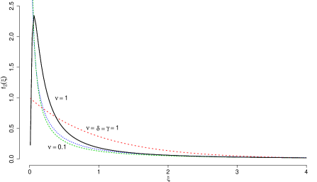
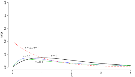
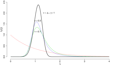
Figure 2: The stretched-squashed Mittag–Leffler density plots (see (3.7)) for parameter values $(\nu,\delta,\lambda,\gamma)=((0.1,0.5,1),2,1,-0.5)$ (top), $(\nu,\delta,\lambda,\gamma)=((0.1,0.5,1),2,1,1)$ (middle), and $(\nu,\delta,\lambda,\gamma)=((0.1,0.5,1),2,1,5)$ (bottom).

Now, consider $m$ i.i.d. random inter-event imes $\Xi_{1},\dots,\Xi_{m}$ of a counting process $\mathcal{N}(t)$, $t\geq 0$, which are distributed according to (3.7). If $W_{m}=\Xi_{1}+\dots+\Xi_{m}$ is the waiting time till the $m$th event, we have

$$\mathbb{E}e^{-sW_{m}}=s^{-m\gamma}\left(\lambda\frac{|\gamma|}{\nu}\right)^{m}{}_{2}\psi_{1}^{m}\left[-\lambda s^{-\nu}\left|\begin{array}[]{l}(1,1),(\gamma,\nu)\\ (\nu,\nu)\end{array}\right.\right].$$ (3.16)

To determine the state probabilities $q_{k}^{\nu}(t)=\Pr\{\mathcal{N}(t)=k\}$, $k\geq 0$, we write

$$\int_{0}^{\infty}e^{-st}q_{k}^{\nu}(t)\,\mathrm{d}t{}= \int_{0}^{\infty}e^{-st}\left(\Pr\{W_{k}<t\}-\Pr\{W_{k+1}<t\}\right)\mathrm{d}t$$ (3.17)

$$={} s^{-k\gamma-1}\left(\lambda\frac{|\gamma|}{\nu}\right)^{k}{}_{2}\psi_{1}^{k}\left[-\lambda s^{-\nu}\left|\begin{array}[]{l}(1,1),(\gamma,\nu)\\ (\nu,\nu)\end{array}\right.\right]$$ (3.20)

$$-s^{-(k+1)\gamma-1}\left(\lambda\frac{|\gamma|}{\nu}\right)^{k+1}\!\!\!{}_{2}\psi_{1}^{k+1}\left[-\lambda s^{-\nu}\left|\begin{array}[]{l}(1,1),(\gamma,\nu)\\ (\nu,\nu)\end{array}\right.\right].$$ (3.23)

3.1 Path generation and parameter estimation

Simulating a sample path of generalization II directly follows from generalization I. Note that the $\Xi$’s can be generated using the algorithm of Cahoy et al. [6]. It is also straighforward to show that the $q$th fractional moment of the random inter-event time is

$$\mathbb{E}\mathcal{T}^{q}=\frac{\pi\Gamma(q\nu/\gamma+1)}{\lambda^{q\nu/\gamma}\Gamma(q/\nu)\sin(\pi q/\nu)\Gamma(1-q)},\qquad 0<q<\nu.$$ (3.24)

Given $m$ renewal times, we propose a formal procedure to estimate the parameters $\nu$, $\gamma$, and $\lambda$ of generalization II. Let $\Xi^{\prime}=\ln(\Xi)$ and $X^{\prime}=\ln(X)$. Following Cahoy et al. [6], we can deduce that

$$\mu_{\Xi^{\prime}}=\mathbb{E}\left(\Xi^{\prime}\right)=\frac{\nu}{\gamma}\left(\frac{-\ln(\lambda)}{\nu}-\eta\right),$$ (3.25)

$$\sigma_{\Xi^{\prime}}^{2}=\left(\frac{\nu}{\gamma}\right)^{2}\left[\pi^{2}\left(\frac{1}{3\nu^{2}}-\frac{1}{6}\right)\right],$$ (3.26)

and

$$\mu_{3}=\mathbb{E}\left(\Xi^{\prime}-\mu_{\Xi^{\prime}}\right)^{3}=-2\zeta(3)\left(\frac{\nu}{\gamma}\right)^{3}.$$ (3.27)

Using the estimating equations above, we can eliminate $\gamma$ and solve for $\nu$ by getting the $2/3$ root of the third central moment and dividing it by the variance. Thus, we obtain

$$\hat{\nu}=\sqrt{\frac{c\pi^{2}}{3\left[\left(2\zeta(3)\right)^{2/3}+\frac{c\pi^{2}}{6}\right]}},$$ (3.28)

where $c=(\hat{\mu}_{3}^{2/3})/\hat{\sigma}_{\Xi^{\prime}}^{2}$. Substituting $\hat{\nu}$ to the variance equation (3.26), we get

$$\hat{\gamma}=\sqrt{\left(\frac{\hat{\nu}}{\hat{\sigma}_{\Xi^{\prime}}^{2}}\right)^{2}\left[\pi^{2}\left(\frac{1}{3\hat{\nu}^{2}}-\frac{1}{6}\right)\right]}.$$ (3.29)

Finally, plugging $\hat{\nu}$ and $\hat{\gamma}$ into the mean equation (3.25) above, we have

$$\hat{\lambda}=\exp\left[-\left(\hat{\mu}_{\Xi^{\prime}}\hat{\gamma}+\eta\hat{\nu}\right)\right].$$ (3.30)

We also tested the above explicit forms of the estimators by calculating the bias and the root-mean-square-error (RMSE) based on the 1000 generated data samples for different parameter and total jump size values. Overall, Table 3 in the appendix showed favorable results for the proposed procedure.

4 Concluding remarks

We proposed two generalizations of the standard and the fractional Poisson processes through their renewal time distributions which naturally provided greater flexibility in modeling real-life renewal processes. Statistical properties such as the state probabilities and process moments were derived. Algorithms to simulate trajectories and to estimate model parameters were also developed. Generally, tests provided additional merits to the proposed procedures.

Although some work have already been done, there are still a few things that need to be pursued. For instance, the complete analysis of the counting process related to the renewal process that has stretched-squashed generalized Mittag–Leffler distributed waiting times would be a worthy pursuit. Also, the development of estimators using likelihood approaches would be of interest as well.

5 Appendix

		Bias			RMSE
$\nu$	$Est$	$m=100$	$1000$	$10000$	$m=100$	$1000$	$10000$
$0.5$	$\hat{\nu}$	0.018	0.001	0.000	0.184	0.049	0.013
	$\hat{\delta}$	0.082	0.011	0.002	0.253	0.074	0.023
	$\hat{\lambda}$	0.207	0.027	0.003	0.525	0.151	0.048
$0.6$	$\hat{\nu}$	0.026	0.003	0.000	0.210	0.068	0.016
	$\hat{\delta}$	0.065	0.010	0.000	0.205	0.074	0.023
	$\hat{\lambda}$	0.174	0.026	0.001	0.442	0.151	0.047
$0.7$	$\hat{\nu}$	0.024	0.001	0.000	0.254	0.056	0.018
	$\hat{\delta}$	0.069	0.009	0.000	0.207	0.067	0.023
	$\hat{\lambda}$	0.176	0.022	0.001	0.434	0.135	0.046
$0.8$	$\hat{\nu}$	0.005	0.003	0.000	0.264	0.077	0.020
	$\hat{\delta}$	0.080	0.008	0.001	0.199	0.072	0.023
	$\hat{\lambda}$	0.202	0.022	0.004	0.429	0.147	0.047
$0.95$	$\hat{\nu}$	0.022	0.001	0.000	0.349	0.079	0.021
	$\hat{\delta}$	0.070	0.009	0.002	0.187	0.067	0.022
	$\hat{\lambda}$	0.184	0.024	0.004	0.405	0.135	0.044

Table 2: Parameter estimates for generalization I using different values of $\nu$, $\delta=0.5$, and $\lambda=0.5$ for total jump sizes $m=100,1000,10000$.

		Bias			RMSE
$\nu$	$Est$	$m=100$	$1000$	$10000$	$m=100$	$1000$	$10000$
$0.5$	$\hat{\nu}$	0.217	0.079	-0.022	0.280	0.176	0.124
	$\hat{\gamma}$	-0.038	-0.016	0.001	0.072	0.034	0.016
	$\hat{\lambda}$	-0.041	-0.014	0.006	0.090	0.044	0.030
$0.6$	$\hat{\nu}$	0.136	-0.021	0.000	0.222	0.153	0.100
	$\hat{\gamma}$	-0.026	0.018	0.051	0.067	0.032	0.016
	$\hat{\lambda}$	-0.017	0.005	0.001	0.085	0.041	0.023
$0.7$	$\hat{\nu}$	0.052	-0.022	-0.008	0.188	0.149	0.060
	$\hat{\gamma}$	-0.015	0.001	0.001	0.071	0.034	0.013
	$\hat{\lambda}$	-0.003	0.007	0.002	0.086	0.040	0.014
$0.8$	$\hat{\nu}$	-0.013	-0.030	-0.003	0.172	0.129	0.034
	$\hat{\gamma}$	0.004	0.006	0.001	0.073	0.035	0.011
	$\hat{\lambda}$	0.007	0.008	0.000	0.086	0.035	0.009
$0.95$	$\hat{\nu}$	-0.043	-0.004	0.000	0.131	0.044	0.013
	$\hat{\gamma}$	0.021	0.002	0.000	0.083	0.028	0.008
	$\hat{\lambda}$	0.014	0.002	0.000	0.073	0.022	0.007

Table 3: Parameter estimates for generalization II using different values of $\nu$, $\lambda=0.5$, and $\gamma=0.5$ for total jump sizes $m=100,1000,10000$.

References

- Laskin [2003] N Laskin. Fractional Poisson process. Communications in Nonlinear Science and Numerical Simulation, 8(3-4):201–213, 2003.
- Laskin [2009] N Laskin. Some applications of the fractional Poisson probability distribution. Journal of Mathematical Physics, 50(11):113513, 2009.
- Uchaikin et al. [2008] VV Uchaikin, DO Cahoy, and RT Sibatov. Fractional Processes: from Poisson to branching one. International Journal of Bifurcation and Chaos, 18(9):2717–2725, 2008.
- Beghin and Orsingher [2009] L Beghin and E Orsingher. Fractional Poisson processes and related planar random motions. Electronic Journal of Probability, 14(61):1790–1826, 2009.
- Beghin and Orsingher [2010] L Beghin and E Orsingher. Poisson-type processes governed by fractional and higher-order recursive differential equations. Electronic Journal of Probability, 15(22):684–709, 2010.
- Cahoy et al. [2010] DO Cahoy, VV Uchaikin, and WA Woyczynski. Parameter estimation for fractional Poisson processes. Journal of Statistical Planning and Inference, 140(11):3106–3120, 2010.
- Mainardi et al. [2004] F Mainardi, R Gorenflo, and E Scalas. A fractional generalization of Poisson processes. Vietnam Journal of Mathematics, 32:53–64, 2004.
- Mainardi et al. [2005] F Mainardi, R Gorenflo, and A Vivoli. Renewal processes of Mittag–Leffler and Wright type. Fractional Calculus and Applied Sciences, 8:7–38, 2005.
- Uchaikin and Sibatov [2008] VV Uchaikin and RT Sibatov. A fractional Poisson process in a model of dispersive charge transport in semiconductors. Russian Journal of Numerical Analysis and Mathematical Modelling, 23(3):283–297, 2008.
- Meerschaert et al. [2010] MM Meerschaert, E Nane, and P Vellaisamy. The fractional Poisson process and the inverse stable subordinator. Electronic Journal of Probability, 16:1600–1620, 2010.
- Politi et al. [2011] M Politi, T Kaizoji, and E Scalas. Full characterization of the fractional Poisson process. Europhysics Letters, 26(2):20004, 2011.
- Scalas [2011] E Scalas. A class of CTRWs: Compound fractional Poisson processes. In J Klafter and R Metzler, editors, Fractional Dynamics: Recent Advances, chapter 15, pages 353–374. World Scientific Publishing Company, Singapore, 2011.
- Scalas [2012] E Scalas. On the convergence of quadratic variation for compound fractional Poisson processes. Fractional Calculus and Applied Analysis, 15(2):314–331, 2012.
- Repin and Saichev [2000] ON Repin and AI Saichev. Fractional Poisson law. Radiophysics and Quantum Electronics, 43:738–741, 2000.
- Uchaikin and Zolotarev [1999] VV Uchaikin and VM Zolotarev. Chance and Stability: Stable Distributions and their Applications. VSP, The Netherlands, 1999.
- Piryatinska et al. [2005] A Piryatinska, AI Saichev, and WA Woyczynski. Models of anomalous diffusion:the subdiffusive case. Physica A: Statistical Physics, 349:375–420, 2005.
- Cahoy and Polito [2012] DO Cahoy and F Polito. Simulation and estimation for the fractional Yule process. Methodology And Computing In Applied Probability, 14(2):383–403, 2012.
- Pillai [1990] RN Pillai. On Mittag-Leffler Functions and Related Distributions. Annals of the Institute of Statistical Mathematics, 42(1):157–161, 1990.
- Saigo et al. [2004] M Saigo, RK Saxena, and AA Kilbas. Generalized Mittag–Leffler function and generalized fractional calculus operators. Integral Transforms and Special Functions, 15(1):31–49, 2004.
- Prabhakar [1971] TR Prabhakar. A singular integral equation with a generalized Mittag–Leffler function in the kernel. Yokohama Mathematical Journal, 19:7–15, 1971.
- Mathai and Haubold [2008] AM Mathai and HJ Haubold. Special Functions for Applied Scientists. Springer, New York, 2008.
- Haubold et al. [2011] HJ Haubold, AM Mathai, and RK Saxena. Mittag–Leffler Functions and Their Applications. Journal of Applied Mathematics, 2011(298628):51, 2011.
- Diethelm [2004] K Diethelm. The Analysis of Fractional Differential Equations. Springer, 2004.
- Srivastava and Tomovski [2009] HM Srivastava and Ž Tomovski. Fractional calculus with an integral operator containing a generalized mittag–leffler function in the kernel. Applied Mathematics and Computation, 211(1):198–210, 2009.